50
Dr Ian R. Manchester Dr Ian R. Manchester Amme 3500 : Root Locus Design
| Date post: | 07-May-2018 |
| Category: |
Documents |
| Upload: | hoangkhuong |
| View: | 213 times |
| Download: | 0 times |

Dr Ian R. Manchester
Dr Ian R. Manchester Amme 3500 : Root Locus Design

Slide 2 Dr. Ian R. Manchester Amme 3500 : Introduction
Week Content Notes 1 Introduction 2 Frequency Domain Modelling 3 Transient Performance and the s-plane 4 Block Diagrams 5 Feedback System Characteristics Assign 1 Due 6 Root Locus 7 Root Locus 2 Assign 2 Due 8 Bode Plots 9 Bode Plots 2 10 State Space Modeling Assign 3 Due 11 State Space Design Techniques 12 Advanced Control Topics 13 Review Assign 4 Due

Slide 3 Dr Ian R. Manchester Amme 3500 : Root Locus Design
• In lecture 5 we had a brief introduction to the classic PID controller
• We will now re-examine the design of these controllers in light of the root locus techniques we have studied
• The complete three-term controller is described by
Kp+Ki/s+Kds -
+
R(s) E(s) C(s) G(s)

Slide 4 Dr Ian R. Manchester Amme 3500 : Root Locus Design
• We have seen how we can use the Root Locus for designing systems to meet performance specifications
• The root locations are important in determining the nature of the system response
• By manipulating the System Gain K we showed how we could change the closed loop transient response
• What if our desired performance specification doesn’t exist on the Root Locus?

Slide 5 Dr Ian R. Manchester Amme 3500 : Root Locus Design
* N.S. Nise (2004) “Control Systems
Engineering” Wiley &
Sons

Slide 6 Dr Ian R. Manchester Amme 3500 : Root Locus Design
• Recall that the transient system specifications can be formulated in the s-plane
Tr ! 0.6 sec
Mp ! 10%
Ts ! 3 sec
sin-1!"
#"
$n
Im(s)
Re(s)
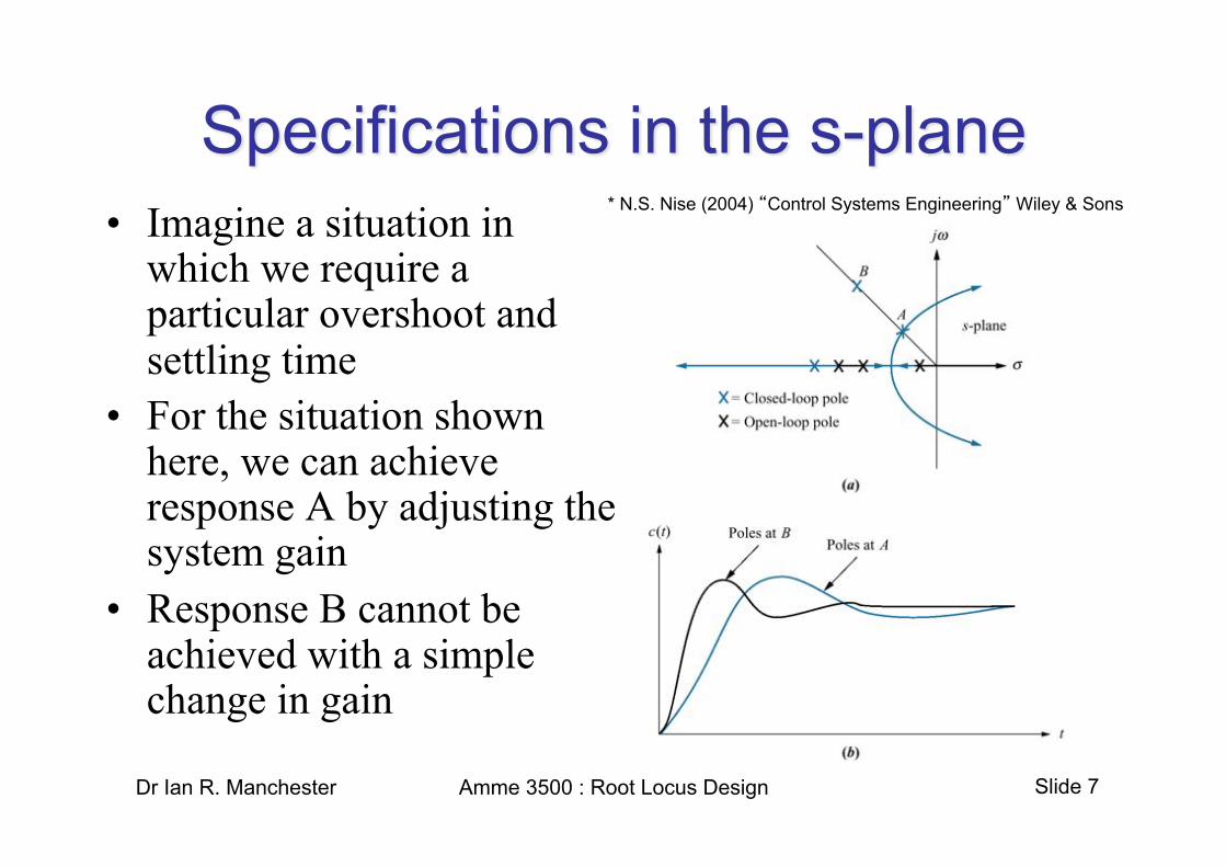
Slide 7 Dr Ian R. Manchester Amme 3500 : Root Locus Design
• Imagine a situation in which we require a particular overshoot and settling time
• For the situation shown here, we can achieve response A by adjusting the system gain
• Response B cannot be achieved with a simple change in gain
* N.S. Nise (2004) “Control Systems Engineering” Wiley & Sons

Slide 8 Dr Ian R. Manchester Amme 3500 : Root Locus Design
• We will now look at the derivative term which can be used to change the transient response
• This is called an Ideal Derivative Compensator
Kp+Kds -
+
R(s) E(s) C(s) G(s)

Slide 9 Dr Ian R. Manchester Amme 3500 : Root Locus Design
• The ideal derivative compensator adds a pure differentiator to the forward path of the control system
• This is effectively equivalent to an additional zero
• As you should by now be aware, the location of the open loop poles and zeros affects the root locus and hence the transient response of the closed loop system

Slide 10 Dr Ian R. Manchester Amme 3500 : Root Locus Design
• Consider a simple second order system whose root locus looks like this (roots -1, -2)
• Adding a zero to this system drastically changes the shape of the root locus
• The position of the zero will also change the shape and hence the nature of the transient response
Zero at -3
Zero at -5

Slide 11 Dr Ian R. Manchester Amme 3500 : Root Locus Design
Uncompensated system
Zero at -2
* N.S. Nise (2004) “Control Systems Engineering” Wiley & Sons

Slide 12 Dr Ian R. Manchester Amme 3500 : Root Locus Design
Zero at -4
Zero at -3
* N.S. Nise (2004) “Control Systems Engineering” Wiley & Sons

Slide 13 Dr Ian R. Manchester Amme 3500 : Root Locus Design
• As the zero moves to the left in the s-plane, it has less effect on the transient response of the system
• In the limit as the zero moves left, the response will be identical to the uncompensated system
* N.S. Nise (2004) “Control Systems Engineering” Wiley & Sons

Slide 14 Dr Ian R. Manchester Amme 3500 : Root Locus Design
• It’s clear that the nature of the response will change as a function of the zero location
• How can we use this information to help us design for a particular specification?
• We can select the location of the additional zero based on the angle criteria to meet our design goal

Slide 15 Dr Ian R. Manchester Amme 3500 : Root Locus Design
• Given the system shown on the right, we’d like to design a compensator to yield a 16% overshoot with a 3 fold reduction in settling time
• The settling time is
* N.S. Nise (2004) “Control Systems Engineering” Wiley & Sons

Slide 16 Dr Ian R. Manchester Amme 3500 : Root Locus Design
• Based on this root location, we can find the desired location for the compensated poles
• We’d like to reduce settling time by 1/3 so
* N.S. Nise (2004) “Control Systems Engineering” Wiley & Sons

Slide 17 Dr Ian R. Manchester Amme 3500 : Root Locus Design
• By the angle criteria
• Based on this we can compute the required zero location, zc
• so zc = 3.006 zc
%c %2 %1
* N.S. Nise (2004) “Control Systems Engineering” Wiley & Sons

Slide 18
• What value of K will put the roots at the desired location?
• Recall that the RL is the location of the closed loop poles but is based on the open loop locations
• We can solve this for K for the compensated system given the desired root location
• So
Dr Ian R. Manchester Amme 3500 : Root Locus Design
!
1+KG = 0
!
K =1G

Slide 19
• For our system, we have
Dr Ian R. Manchester Amme 3500 : Root Locus Design
!
K =1
s+ 3.006s(s+ 4)(s+ 6) s="3.613+6.193 j
=s(s+ 4)(s+ 6)s+ 3.006 s="3.613+6.193 j
=("3.613+ 6.193 j)(0.387 + 6.193 j)(2.387 + 6.193 j)
("0.608 + 6.193 j)= 47.45
Slide 20 Dr Ian R. Manchester Amme 3500 : Root Locus Design
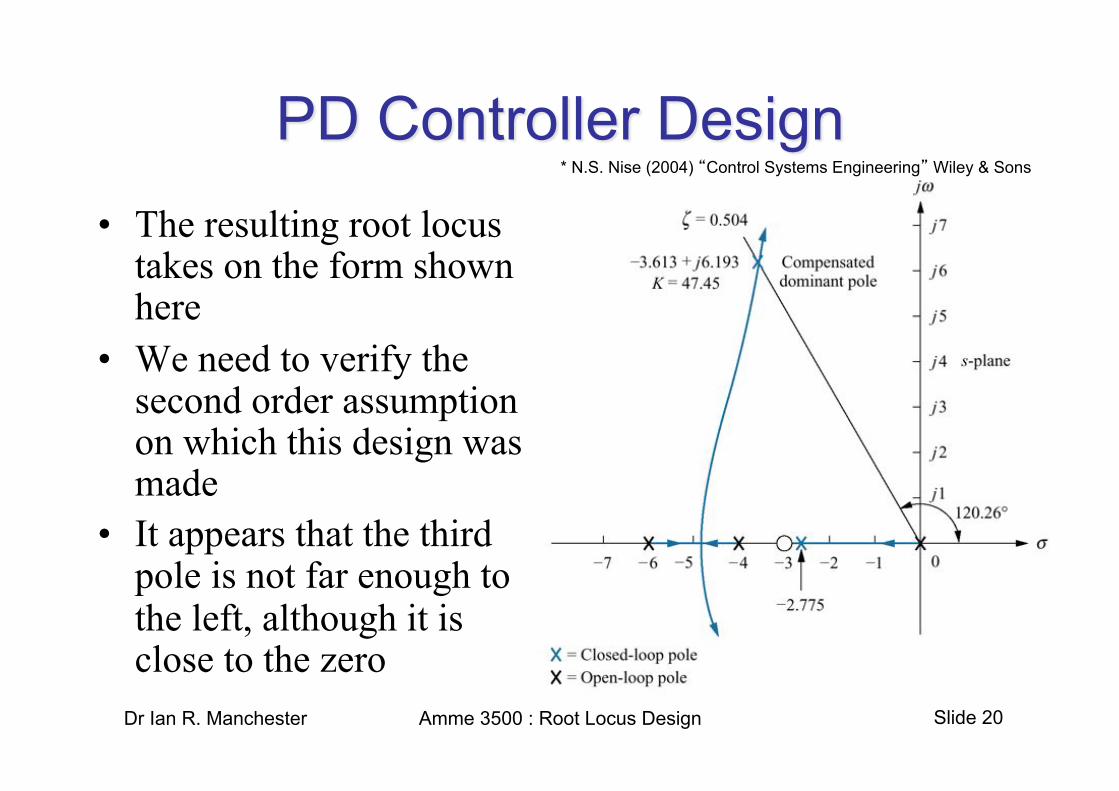
• The resulting root locus takes on the form shown here
• We need to verify the second order assumption on which this design was made
• It appears that the third pole is not far enough to the left, although it is close to the zero
* N.S. Nise (2004) “Control Systems Engineering” Wiley & Sons

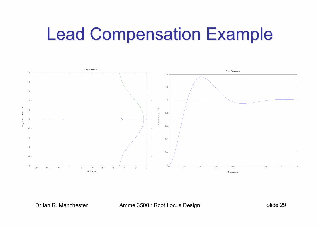
Slide 21 Dr Ian R. Manchester Amme 3500 : Root Locus Design
• A simulation of the resulting step response is required to verify the design
• The resulting step response demonstrates a threefold improvement in settling time with a 3% difference in overshoot
* N.S. Nise (2004) “Control Systems Engineering” Wiley & Sons

Slide 22 Dr Ian R. Manchester Amme 3500 : Root Locus Design
• In practice, we often don’t want to implement a pure differentiator
• A pure PD controller requires active components to realize the differentiation
• The differentiation will also tend to amplify high frequency noise
Slide 23 Dr Ian R. Manchester Amme 3500 : Root Locus Design
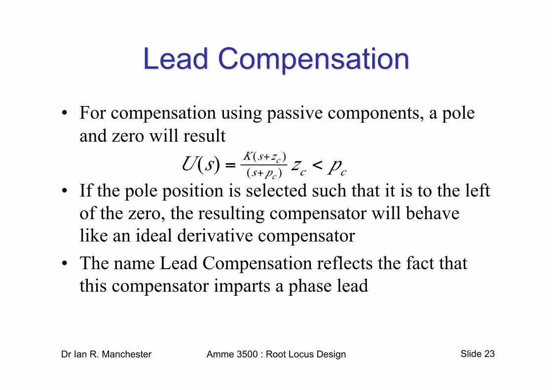
• For compensation using passive components, a pole and zero will result
• If the pole position is selected such that it is to the left of the zero, the resulting compensator will behave like an ideal derivative compensator
• The name Lead Compensation reflects the fact that this compensator imparts a phase lead

Slide 24 Dr Ian R. Manchester Amme 3500 : Root Locus Design
• In this case there won’t be a unique zero location that yields the desired system response
• Selecting the exact values of the pole and zero location is usually an iterative process
• Each iteration considers the performance of the resulting system
• The choice of pole location is a compromise between the conflicting effects of noise suppression and compensation effectiveness

Slide 25 Dr Ian R. Manchester Amme 3500 : Root Locus Design
• Find a compensation for
• That will provide overshoot of no more than 20% and a rise time no more than 0.25s
• Noise suppression requirements require that the lead pole be no larger than 20

Slide 26 Dr Ian R. Manchester Amme 3500 : Root Locus Design
• First find a point in the s-plane that we’d like to have on the root locus
• Place the lead pole at -20 and solve for the position of the zero
x
%1=120 %2=112.4 %3=20.2 %c=72.6

Slide 27 Dr Ian R. Manchester Amme 3500 : Root Locus Design

Slide 28 Dr Ian R. Manchester Amme 3500 : Root Locus Design
• We could also have placed the pole at -15, although this is likely to affect the 2nd order assumption
• Place the lead pole at -15 and solve for the position of the zero
x
%1=120 %2=112.4 %3=27.8 %c=80.2
Slide 29 Dr Ian R. Manchester Amme 3500 : Root Locus Design

Slide 30 Dr Ian R. Manchester Amme 3500 : Root Locus Design
• We also looked at how the system type is related to the steady state error of the system for a set of input types
• Systems may not meet our desired steady state error requirements based purely on a proportional controller
• Additional poles at the origin may therefore be required to change the nature of the steady state system response

Slide 31 Dr Ian R. Manchester Amme 3500 : Root Locus Design
* N.S. Nise (2004) “Control Systems Engineering”
Wiley & Sons

Slide 32 Dr Ian R. Manchester Amme 3500 : Root Locus Design
• If we add a zero close the pole at the origin the root locus reverts to approximately the same as the uncompensated case
• The system type has been increased without appreciably affecting the transient response
* N.S. Nise (2004) “Control Systems Engineering” Wiley & Sons

Slide 33 Dr Ian R. Manchester Amme 3500 : Root Locus Design
• We will now look at the integral term used to eliminate steady state error
• This is called an Ideal Integral Compensator
Kp+Ki/s -
+
R(s) E(s) C(s) G(s)
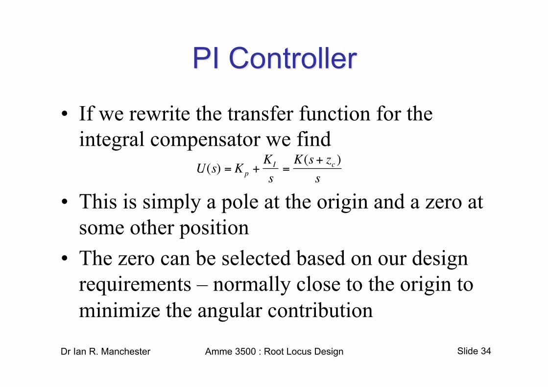
Slide 34 Dr Ian R. Manchester Amme 3500 : Root Locus Design
• If we rewrite the transfer function for the integral compensator we find
• This is simply a pole at the origin and a zero at some other position
• The zero can be selected based on our design requirements – normally close to the origin to minimize the angular contribution
!
U(s) = Kp +KI
s=K(s+ zc )
s

Slide 35 Dr Ian R. Manchester Amme 3500 : Root Locus Design
• Given the system shown here we’d like to add a PI controller to eliminate the steady state error
• We find that
* N.S. Nise (2004) “Control Systems Engineering” Wiley & Sons

Slide 36 Dr Ian R. Manchester Amme 3500 : Root Locus Design
* N.S. Nise (2004) “Control Systems Engineering” Wiley & Sons

Slide 37 Dr Ian R. Manchester Amme 3500 : Root Locus Design
• As with the lead compensation, using passive components results in a pole and zero
• If the pole position is selected such that it is to the right of the zero near the origin, the resulting compensator will behave like an ideal integral compensator although it will not increase the system type
• The name Lag Compensation reflects the fact that this compensator imparts a phase lag
>

Slide 38 Dr Ian R. Manchester Amme 3500 : Root Locus Design
• How does the lag compensator affect the steady state performance?
• If we have a plant of the form
• The static error constant will be
Slide 39 Dr Ian R. Manchester Amme 3500 : Root Locus Design
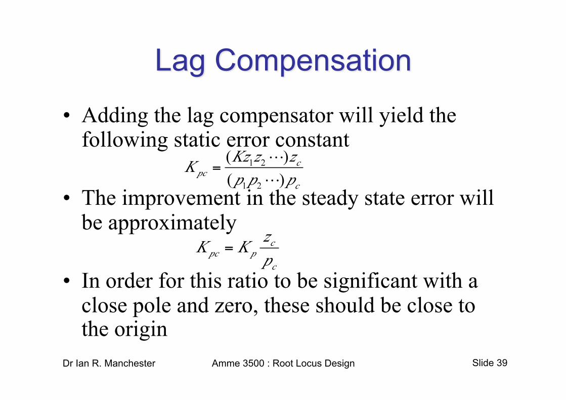
• Adding the lag compensator will yield the following static error constant
• The improvement in the steady state error will be approximately
• In order for this ratio to be significant with a close pole and zero, these should be close to the origin
Slide 40 Dr Ian R. Manchester Amme 3500 : Root Locus Design
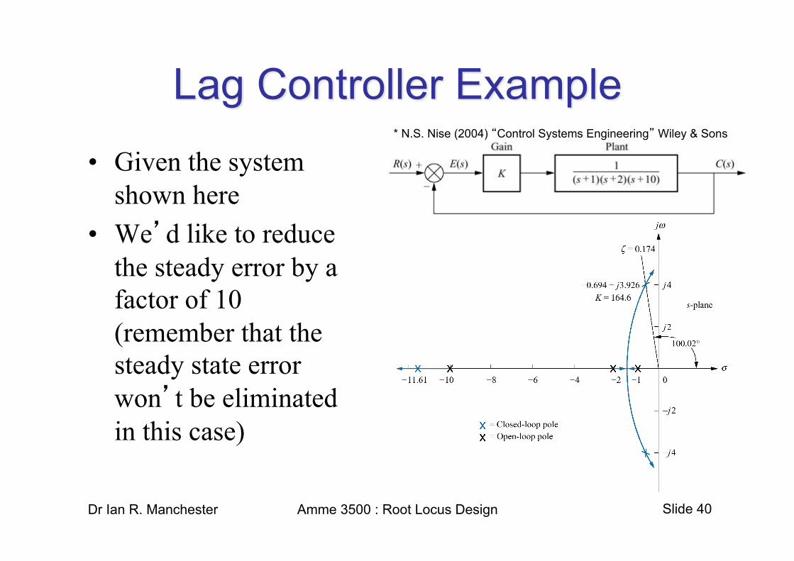
• Given the system shown here
• We’d like to reduce the steady error by a factor of 10 (remember that the steady state error won’t be eliminated in this case)
* N.S. Nise (2004) “Control Systems Engineering” Wiley & Sons

Slide 41 Dr Ian R. Manchester Amme 3500 : Root Locus Design
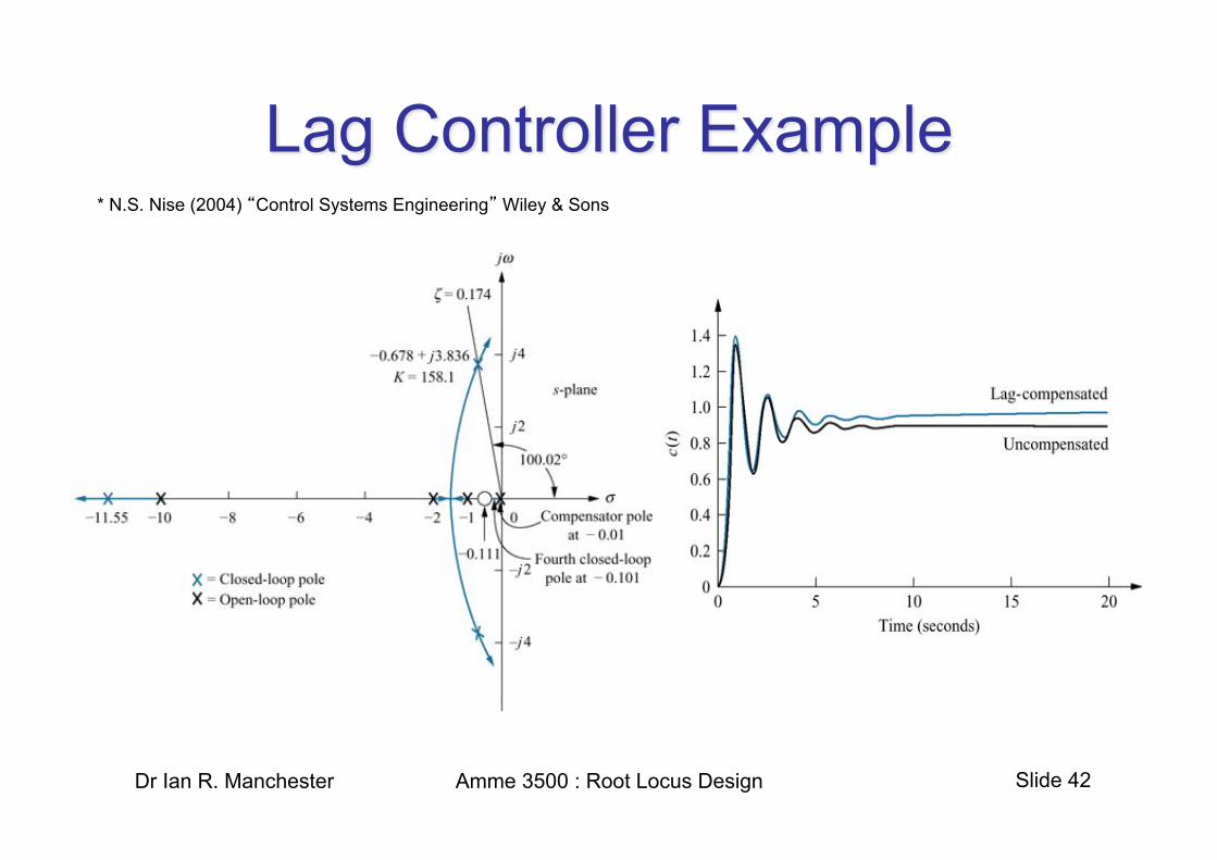
• Previously we found the system error to be 0.108 with Kp=8.23. For a 10 fold improvement
• This requires Kpc=91.6. This implies that
• We therefore require a ratio of approximately 11 between the pole and zero location
• Selecting pc=0.01, zc will be 0.111
Slide 42 Dr Ian R. Manchester Amme 3500 : Root Locus Design
* N.S. Nise (2004) “Control Systems Engineering” Wiley & Sons

Slide 43 Dr Ian R. Manchester Amme 3500 : Root Locus Design
• The design of a PID or Lead/Lag controller consists of the following 8 steps – Evaluate the performance of the uncompensated system to
determine what improvement in transient response is required
– Design the PD/Lead controller to meet the transient response specifications
– Simulate the system to be sure all requirements are met – Redesign if simulation shows that requirements have not
been met

Slide 44 Dr Ian R. Manchester Amme 3500 : Root Locus Design
– Design the PI/Lag controller to yield the required steady-state error
– Determine the gains required to achieve the desired specification
– Simulate the system to be sure that all requirements have been met
– Redesign if simulation shows that requirements have not been met

Slide 45 Dr Ian R. Manchester Amme 3500 : Root Locus Design
!
J ˙ ̇ " = u
G(s) =1Js2

Slide 46
• Aluminium extraction from Bauxite
• slow multi-compartment dynamics
Dr Ian R. Manchester Amme 3500 : Root Locus Design !
G(s) =1
(s+1)(s+ 0.2)(s+ 0.1)
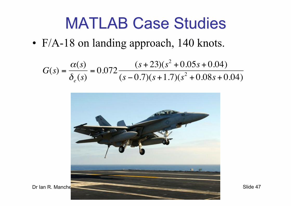
Slide 47
• F/A-18 on landing approach, 140 knots.
Dr Ian R. Manchester Amme 3500 : Root Locus Design
!
G(s) ="(s)#e (s)
= 0.072 (s+ 23)(s2 + 0.05s+ 0.04)(s $ 0.7)(s+1.7)(s2 + 0.08s+ 0.04)

Slide 48 Dr Ian R. Manchester Amme 3500 : Root Locus Design
• The University of Michigan has a very nice set of design examples for a variety of systems
• Have a look at the following URL for details • http://www.engin.umich.edu/group/ctm/index.html

Slide 49 Dr Ian R. Manchester Amme 3500 : Root Locus Design
• We have presented design methods based on the root locus for changing the characteristics of the system response to meet our specifications
• There are many cases in which simple gain adjustment will not be sufficient to meet the specifications
• In these cases, we must introduce additional dynamics into the system to meet our performance requirements

Slide 50 Dr Ian R. Manchester Amme 3500 : Root Locus Design
• Nise – Sections 9.1-9.6
• Franklin & Powell – Section 5.5-5.6


