Draft -- comments welcome. Please do not quote without...

Draft -- comments welcome. Please do not quote without permission

The Impact of Negotiated Restraints on US Trade in Textiles

Patrick Conway Department of Economics

Gardner Hall, CB 3305 University of North Carolina at Chapel Hill

[email protected]

10 November 2004

Abstract: This paper examines the evidence of the effectiveness of the quota system under the MFA and the current ATC in restraining imports into the US. The period considered is 1989-2002, and the goods examined were those in textile quota categories 225 and 314.While there is evidence of individual binding restraints, there is little evidence that the quota system was a significant source of protection to the US producer. The phenomenon of US exports of goods under import quota is also examined. These prove to be quite significant in the two categories considered. This research on textiles trade was initiated with Alfred Field and Robert Connolly of UNC. Thanks to them for their support. They should not be associated with the conclusions of this essay.

Conway: MFA Restraints and Textile Trade - 2

The system of bilateral quantitative restraints (or quotas) on textile and apparel imports into the US has been an enduring feature of the US commercial policy system. From its inception in the early 1960s with the Long-Term Arrangement in Cotton Textiles (LTA), through its codification in the Multi-Fiber Arrangement (MFA) from 1974 to 1995, and to its current form in the Agreement on Textiles and Clothing (ATC), the system has provided protection to US producers of textiles and apparel. In the negotiations that led to the adoption of the ATC in 1995, the US agreed to dismantle the system of quantitative restraints sequentially. A large number of restraints was removed at the beginning of 1995, 1998 and 2002, but those remaining govern trade in the categories of textiles most produced in the US. These remaining restraints are scheduled for removal on 1 January 2005. While there is tremendous concern about the outcome of removal of these restraints, there is little research focused upon this question. The ATC has evolved into a complicated interlocking set of bilateral agreements on quantities exported to the US. They act as voluntary export restraints, but they are binding in any given year on only a small subset of the countries under restraint. Specific limits and group limits interact in non-transparent ways to limit a given country’s exports. A model of the market capable of forecasting the impact of removing these restraints must incorporate all of these features. In this paper I develop such a model. I apply it to the removal of quantitative restraints for US imports in two specific textiles product lines: the collection of fabrics known in the ATC as “blue denim” – category 225 – and “broadwoven cotton fabrics” – category 314. Conclusions on this work remain quite tentative. Among the points deserving greater attention in completion of this paper are that

o There is substantial export activity in textile product lines identical to or quite similar to those covered by the ATC restraints. Much of this export is to Caribbean nations, Mexico and Canada: these serve as alternative assembly platforms for apparel production.

o There is little evidence that the system of restraints was successful in

limiting the quantity imported from the restrained countries. Many of these nevertheless captured increased market share during years under restraint, while those not under restraint often lost market share. This phenomenon occurs even after controlling for level of development and differences in relative cost of the imported product.

o There is some evidence of spillover from binding restraint to non-

restrained countries. This appears to contradict the previous point, but may simply be its complement: ingenious suppliers both found (possibly costly) ways to circumvent the restraints and turned to other suppliers when a binding restraint was looming.


I. Characteristics of the restraints on US textiles imports. The basic unit of the current system is the restraint category, or quota category. These categories are defined as aggregated subgroups of textile and apparel products with some shared characteristic or raw material. The current system of import restraints in the US identifies 11 aggregated categories of yarns, 34 aggregated categories of textiles, 86 categories of apparel and 16 categories of miscellaneous textiles (e.g., towels). Together these categories span the entire set of US textile imports. Each category includes multiple products. For example, category 225 (blue denim) is aggregated from 16 distinct product lines within the harmonized tariff system while category 300 (carded cotton yarn) is aggregated from 25 product lines. 1 This ensures that the products included in each category are similar, but may have significant differences: for example, the “blue denim” category includes denim made from both cotton and man-made fibers. Limits under the system of restraints were divided into specific limits and group limits. Specific limits governed the import of goods within the specific quota category. Group limits placed aggregate limits on a subset of the quota categories. If a country’s exports were subject to group limits but not specific limits, then the suppliers of that country (or more likely, a government agency supervising these exports) could choose any mix of goods shipped to the US so long as in aggregate the totals did not exceed the group limit. Some group limits covered only two quota categories: e.g., group 300/301, covering quota categories 300 (carded cotton yarn) and 301 (combed cotton yarn). Others spanned a large number of categories: for example, Subgroup 1 in Hong Kong included quota categories 200, 226, 313, 314, 315, 369 and 604. In many cases, a country has its exports bound by both specific limits and group limits. Under the MFA and ATC, exporting countries have been given flexibility in meeting these restraints. In each category, the agreement specified a percentage by which the country could either exceed or fall short of its restraint. In those cases, a maximum percent of possible “carryforward” or “carryover” is specified in the agreement. With carryforward, the country transfers part of this year’s quota to the following year. With carryover, the country exceeds its quota in this period by counting the excess against quota in the following year. Not all textiles exporters to the US are subject to quantitative limits. Under the MFA, restraints were negotiated whenever a country’s exports caused (or threatened to cause) market disruption in the US. Table 1 lists the countries in Q 314 and Q 225 for which restraints had been negotiated by 2002. Of the top 20 sources of imported denim (by quantity) only nine are listed. (For two others (Mexico and Canada) restraints were superseded by the North American Free Trade Agreement.)2 Of the top 20 sources of imported broadwoven cotton fabric and poplin in Q 314, the list in Table 1 includes 11 while three (Canada, Mexico, Israel) are governed by free-trade agreements. Five of the countries on the list (Brazil, Macao, Romania, Philippines and Egypt) were not in the top

1 Each product line is represented by a 10-digit harmonized-tariff-system (HTS) code. 2 The other countries, in declining volumes of imports, are Turkey, Pakistan, Italy, Japan, United Arab Emirates, Spain, Mauritius, Australia and Belgium.


20 import sources in 2002, while six countries without restraints in this category were ranked in the top 20.3 In all, of the 52 countries in Q 314 exporting to the US in 2002 only 16 had negotiated restraints; of the 35 countries in Q 225 exporting to the US only 11 had negotiated restraints. Of these, in Q 314 the specific limits were binding for China and Pakistan in 2002.4 Group limits were binding for China, India, Korea and Taiwan in that year. In Q 225 no specific limits were binding in 2002, although China, India and Korea were subject to applicable binding group limits in that year. II. Previous research on these restraints. The ATC and its predecessor MFA have prompted academic research in the past that can be reported in two broad categories. The larger category has included calculations of the quantitative impact of these restraints on welfare in the US. Cline (1987), de Melo and Tarr (1990), and more recently US ITC (2002), illustrate these efforts and document the large costs to consumers associated with the restraints. The smaller category includes papers that examine the quantitative effects of these restraints on the exporting nations. Dean (1990) examines aggregate imports of textiles and clothing products from eight Asian countries during the period 1975-1984, and concludes that the MFA restraints were successful in restraining exports from the targeted countries: in her words, “a controlled country’s import share grew, on average, 56 % more slowly than the share of an uncontrolled country.” (Dean, 1990, p. 69) A number of authors have used computable general-equilibrium models to estimate the impact of the MFA system (and its removal) on developing countries. Trela and Whalley (1990) found that the aggregated system imposed welfare losses upon the developing-country exporters, and calculated a new general-equilibrium outcome for the post-system world economy. Yang et al. (1997) examined the relative growth of textiles exports to the US across developing-country exporters as the system of restraints is discontinued. All regions were forecast to increase textile exports, although Hong Kong, Taiwan and Korea were expected to face reduced demand for apparel as other developing countries expanded market share. Dean (1995) examined the incidence of restraint agreements under the MFA in order to determine the determinants of negotiated restraints.. The MFA, and after that the ATC, called for restraints to be negotiated on categories of textiles and apparel imported into the US if a country’s exports caused or threatened to cause market disruption in the US. Dean concluded that in the early years of the MFA (1974-1977) this was in fact the case – exporters individually responsible for large shares of US imports were targeted with these restrictions. In the later years of the MFA (1978-1985), the restraints were introduced upon countries representing much smaller shares of total US imports. These,

3 These six were, in declining volumes of imports, United Arab Emirates, Bahrain, Japan, Italy, Spain and Uzbekistan. 4 The definition of “binding” that I will use in this paper is that of Dean (1990): exports from that country to the US were at least 90 percent of the restraint limit in that year.


according to Dean, may have been designed to target the threat of disruption rather than an actual disruption.5 Evans and Harrigan (2003) investigated the sourcing of apparel imports into the US under the constraints of the MFA. They used a simple model of import sourcing with three determinants: a country-specific effect, a “trade frictions” variable dependent upon tariffs and transport costs, and an interactive term of distance and a replenishment coefficient. Their central hypothesis relates to the hypothesis of “lean retailing” from Abernathy et al. (1999) – that retailers will source rapid-replenishment goods in closer locations to ensure quick availability – and they estimated this in a model that admits the impact of quota restrictions. They separated apparel imports into categories, and identify each category either as “rapid replenishment” or not. They concluded that import growth in rapid-replenishment goods was significantly larger in local suppliers, thus supporting the lean retailing hypothesis. Panagariya et al. (2001) estimated a demand system for apparel exports from Asia to the US. They used the fact that restraints were binding to simplify the typical demand system: quantities were treated as exogenous, and prices as endogenous. The MFA system was not itself the subject of the analysis, but the maintained hypothesis. The authors conclude that within this system the price elasticities of demand for textiles and apparel in the US are quite high: for example, they estimated a price elasticity of 26 for Bangladesh’s textiles and apparel exports to the US. These studies share three features of the market for textiles that are inconsistent with current experience. First, the notion that exports under a binding restraint can be treated as exogenous quantities requires greater investigation, given the flexibility with which the exporting countries can approach these restraints. Second, the idea that imports can be examined without regard to US exports is troublesome in a world in which exports of some textiles categories exceed both imports and domestic production. Third, an analysis that aggregates textiles and apparel, or all apparel, will miss a substantial amount of variation in the more disaggregated data. As Evans and Harrigan (2003) illustrated, there are significant differences among categories of textiles and apparel; these should be exploited and incorporated in the analysis. In what follows I re-consider each of these. I work with the most disaggregated data consistent with the MFA/ATC restraint system by considering imports at the level of two quota categories for textiles imports. This allows for calculation of coherent unit value statistics, since all imports in these two categories are measured in the same units (square meters). I introduce the complementarity of binding specific limits and binding group limits while modeling that substitution possible under this system. I calculate the US exports undertaken in textiles categories analogous to those covered by the MFA/ATC restraint system and examine the interplay of imports and exports.

5 It’s also the case that restraints, once introduced, have not been removed. Thus, the “second wave” of restraints would have to be on smaller exporters, even if the policy goal is to restrain the largest exporters remaining unrestrained.


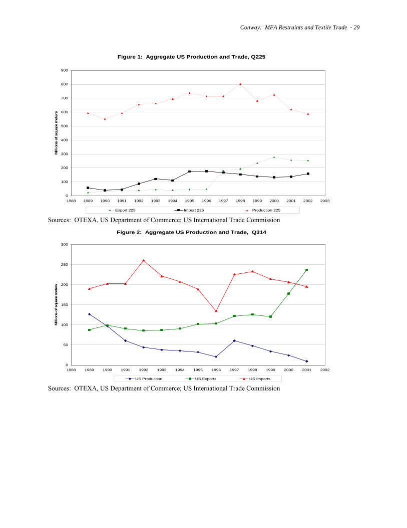
III. US Production and Trade in Q 314 and Q 225. Figures 1 and 2 illustrate US production, export and import of textiles in the categories Q 225 and Q 314, respectively; measurements are in square meters.6 For blue denim, production was relatively stable throughout the period 1989-2002. It rose through 1998, and declined thereafter until the 2002 quantity roughly matched that observed in 1989. For broadwoven cotton, production declined steadily through 1996, jumped temporarily in 1997, and then declined through 2001.7 Imports in these two categories were both substantial and somewhat volatile. In Q 314 the quantity imported oscillated between 140 and 260 million square meters per year during the period 1989-2001. In Q 225 imports were quite small relative to production in 1989, but rose in volume through 1995. From 1995 to 2002 the quantity imported was roughly constant. The degree of US export in these two quota categories is a surprising feature of US textiles trade.8 In Q 314, the quantity exported rose rapidly and exceeded the quantity imported by 2001. In Q 225, the quantity exported exceeded the quantity imported from 1997 forward. This imbalance is even most striking when measured in value terms, as illustrated in Figure 3. In both categories the ratio of export value to import value rose above 1 by 1997. An important reason for this export dominance is the relatively higher unit value of the products exported when compared with the average unit value of imported products. This is evident in Figure 4. US exports in both categories have a similar average value of $2.25 per square meter. However, US imports of denim are available for average value of $1.50 per square meter, and US imports of broadwoven cotton enter for no more than $0.75 per square meter on average.9 Trading blocs. US trade in these two categories of textiles is dominated by trade with three sets of trading partners. The first bloc is that of the North American Free Trade Agreement (NAFTA): Mexico and Canada are dominant trading partners in both

6 Data are drawn from two sources. The OTEXA Division of the International Trade Administration, US Department of Commerce, provides a quarterly report entitled “US Imports, Production Markets, Import Production Ratios and Domestic Market Shares for Textile and Apparel Product Categories” that includes production and imports. The US International Trade Commission provides data on export and import by 10-digit HTS product line that can be aggregated to correspond to the textile quota categories. The import data from the two sources correspond well, and so the US ITC data are reported for export and import. 7 Production statistics are not reported for 2002. There were so few producers still remaining in this category that the Census Bureau cannot release statistics for reasons of confidentiality. 8 Export categories are not explicitly defined by the ATC. I create the quantity and value of exports by aggregating all 10-digit HTS categories that correspond to identical descriptions of product to that in the quota category. For example, the Q 225 category includes HTS 5209.42.0020 and HTS 5209.42.0040. The export category includes these as well as HTS 5209.42.0030 and HTS 5209.42.0050 with very similar descriptions. 9 These values do not include freight, tariff and handling charges in the US, so that the gap between the products landed in the US and the US export products will not be as large.


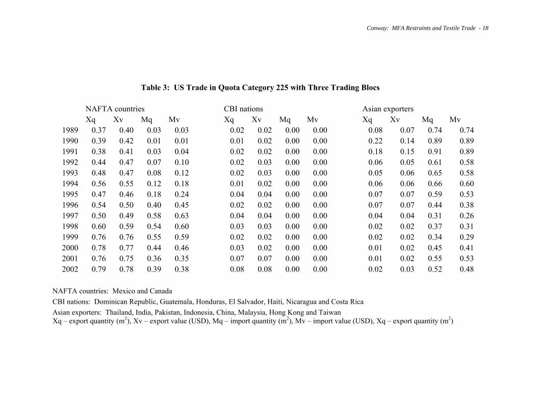
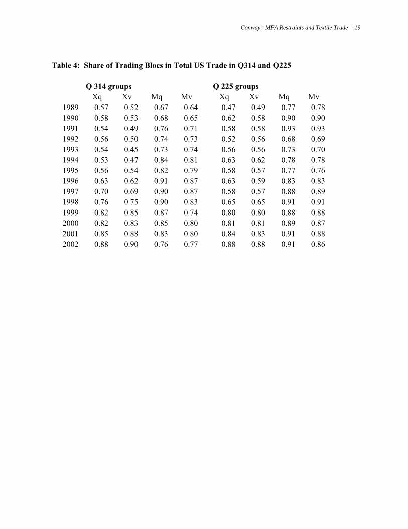
exports and imports of Q 225, and in exports of Q 314.10 The second bloc is the Caribbean Basin Initiative (CBI) group. The Caribbean Basin Initiative provides quota-free and customs duty-free entry to the United States on a permanent basis for apparel assembled from US-made yarns and fabrics.11 The most recent piece of CBI legislation, the Caribbean Basin Trade Partnership Act (CBTPA), provides beneficiary countries certain trade benefits similar to Mexico's under NAFTA. Although the CBI nations represent a miniscule share of US imports, they represent a large share of US exports in Q 314. The third bloc is made up of the Asian exporters: they are a miniscule share of US exports, but a dominant source of imports. Table 2 reports the shares of trade in Q314 to and from these blocs, while Table 3 reports the shares of trade in Q 225 with these blocs. In the trade of Q 314 given in Table 2, the US receives a majority of its imports (both in quantity and in value terms) from six Asian exporters: Thailand, India, Pakistan, Indonesia, China and Malaysia. It ships the majority of exports in this category to qualified countries of the CBI. The NAFTA nations are also a substantial target for US exports, but provide almost none of the US imports. In the trade of Q 225 summarized in Table 3, NAFTA countries represent a much larger share. The Asian exporters are a source of roughly half of US imports (as opposed to three quarters in Q 314), but once again are a target of almost none of US exports.12 The CBI nations are much less important as targets for the denim of Q 225. All of the Asian exporters are, and have been, subject to quotas under the ATC (and previously, under the MFA). While the imports and exports are in principle different goods – if only because the CBI treatment of apparel requires US provenance of the cloth used as raw material – the material balances in broadwoven cotton tell an intriguing story. As Figure 1 illustrates, US exports of cloth in this category have exceeded US production of such cloth since 1990. Given the large mark-up between import unit value and export unit value, it would be natural for the domestic producers to swap out domestic production and replace it with cloth from foreign sources. It is impossible to show that such activity is taking place, but the material balances are highly suggestive. Changing shares of imports. In Figure 5, the share of imports in Q 314 by each trading country (in quantity terms) is plotted for 1989 and for 1996. Observations below the diagonal represent countries increasing their share of imports into the US during this

10 Prior to 1996, Canada was the larger of the two as a source of US imports in Q 225; given that imports from Canada were relatively more expensive than the average imports, the value share of imports exceeded the quantity share of imports for the two. After 1996, Mexico became the larger partner. In 2002, imports from Mexico were three times larger in value than imports from Canada. Mexico and Canada have been the largest two destinations for US export of denim throughout the period 1989-2002. Prior to 1998 Canada was the larger, but since that time has been the smaller destination. In 2002 Mexico was 4.4 times larger in value terms as a destination for US exports of blue denim. 11 The Caribbean Basin Economic Recovery Act of 1983 (CBERA) (amended in 1990) and the Caribbean Basin Trade Partnership Act of 2000 (CBTPA) are collectively known as the Caribbean Basin Initiative (CBI). 12 Notice that the Asian exporters considered in Table 3 include Hong Kong and Taiwan. These two represented a substantial share of US denim imports during the period under consideration.


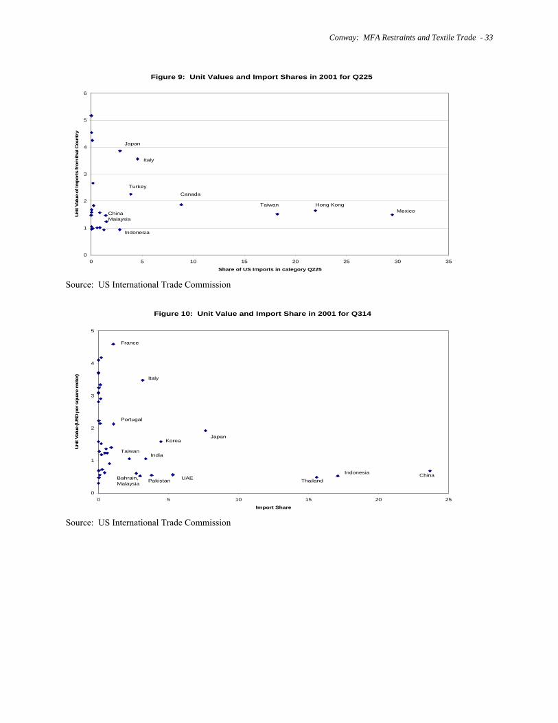
period, while observations above the diagonal indicate countries losing market share. Major sources of imports are indicated by country name. It is evident that during this period Indonesia, Thailand, Malaysia and India captured increased market share. Taiwan and Korea, and to a lesser extent Japan, France and the UK, ceded market share. Of these countries increasing market share, all four were subject to restraint under the MFA from 1988 forward. The restraints on Indonesia and Thailand were binding in 1988, on Malaysia in 1990, and on India by 1992. Nevertheless, the four captured market share during the period. In 1996, the countries subject to binding restraint were China and India. Figure 6 examines the evolution of market share in Q 314 for the period 1996-2001. The major gains in market share for the period 1996-2001 accrued to China. Pakistan. UAE and Bahrain also gained market share, albeit less spectacularly. The country ceding market share was predominantly Malaysia, although Japan lost to a lesser extent. The restraint on these latter two was not binding in 1996 (or indeed, in any year past 1991 under the MFA). Figures 7 and 8 provide similar summaries of the evolution of import shares in Q 225. The major story in the evolution of import shares from 1989 to 1996 was the explosion in imports from Mexico and Canada. These two sources went from minimal market share to 40 percent between them; Hong Kong, Taiwan, Brazil and Argentina were the major losers in market share during this period. Brazil was subject to binding restraints for most of the intervening years. Hong Kong and Taiwan’s exports were subject to group restraints (i.e., covering not only Q 225, but Q317, Q326 and Q 218 (for Hong Kong) as well). It is evident in Figure 8 that Mexico and Canada largely retained market share from 1996 to 2001. Hong Kong and Taiwan recaptured lost market share at the expense of countries such as Brazil, Pakistan, Spain and India. Of these latter, only India and Brazil were subject to restraint during the period, and only in India was the restraint binding. The absence of China from these Q 225 diagrams is quite striking, given the attention paid to China in recent trade discussions. Blue denim is one category within a group restraint on Chinese cloth. While blue-denim exports are rather small, the Chinese exporters specialize in the other components of the group. The group restraint was binding for 1988 through 2002. Import cost. Figures 9 and 10 report the shares of US imports in the two categories coming from various exporting countries: these shares will thus coincide with those reported in Figures 6 and 8. Also presented in these figures are the unit values of cloth imported into the US in these categories. In both categories, the countries with largest import share are those with relatively low unit value. In Q 225, these countries are not the lowest-cost producers, but remain substantially lower in cost than other major providers Canada, Japan, Turkey and Italy. In Q 314, by contrast, the major producers are also the lowest-cost sources. Japan,


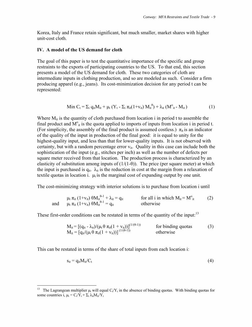
Korea, Italy and France retain significant, but much smaller, market shares with higher unit-cost cloth. IV. A model of the US demand for cloth The goal of this paper is to test the quantitative importance of the specific and group restraints to the exports of participating countries to the US. To that end, this section presents a model of the US demand for cloth. These two categories of cloth are intermediate inputs in clothing production, and so are modeled as such. Consider a firm producing apparel (e.g., jeans). Its cost-minimization decision for any period t can be represented: Min Ct = Σi qitMit + µt (Yt - Σi πit(1+vit) Mit

θ) + λit (Moit - Mit ) (1)

Where Mit is the quantity of cloth purchased from location i in period t to assemble the final product and Mo

it is the quota applied to imports of inputs from location i in period t. (For simplicity, the assembly of the final product is assumed costless.) πit is an indicator of the quality of the input in production of the final good: it is equal to unity for the highest-quality input, and less than that for lower-quality inputs. It is not observed with certainty, but with a random percentage error vit. Quality in this case can include both the sophistication of the input (e.g., stitches per inch) as well as the number of defects per square meter received from that location. The production process is characterized by an elasticity of substitution among inputs of (1/(1-θ)). The price (per square meter) at which the input is purchased is qit. λit is the reduction in cost at the margin from a relaxation of textile quotas in location i. µt is the marginal cost of expanding output by one unit. The cost-minimizing strategy with interior solutions is to purchase from location i until µt πit (1+vit) θMit

θ-1 + λit = qit for all i in which Mit = Moit (2)

and µt πit (1+vit) θMitθ-1 = qit otherwise

These first-order conditions can be restated in terms of the quantity of the input:13

Mit = [(qit - λit)/(µt θ πit(1 + vit))](1/(θ-1))

for binding quotas (3) Mit = [qit/(µt θ πit(1 + vit))] (1/(θ-1)) otherwise This can be restated in terms of the share of total inputs from each location i: sit = qitMit/Ct (4)

13 The Lagrangean multiplier µt will equal Ct/Yt in the absence of binding quotas. With binding quotas for some countries i, µt = Ct/Yt + Σi λitMit/Yt


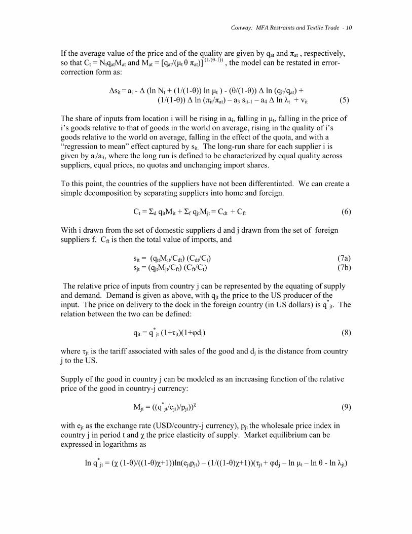
If the average value of the price and of the quality are given by qat and πat , respectively, so that Ct = NtqatMat and Mat = [qat/(µt θ πat)] (1/(θ-1)) , the model can be restated in error-correction form as: ∆sit = ai - ∆ (ln Nt + (1/(1-θ)) ln µt ) - (θ/(1-θ)) ∆ ln (qit/qat) + (1/(1-θ)) ∆ ln (πit/πat) – a3 sit-1 – a4 ∆ ln λt + vit (5) The share of inputs from location i will be rising in ai, falling in µt, falling in the price of i’s goods relative to that of goods in the world on average, rising in the quality of i’s goods relative to the world on average, falling in the effect of the quota, and with a “regression to mean” effect captured by sit. The long-run share for each supplier i is given by ai/a3, where the long run is defined to be characterized by equal quality across suppliers, equal prices, no quotas and unchanging import shares. To this point, the countries of the suppliers have not been differentiated. We can create a simple decomposition by separating suppliers into home and foreign. Ct = Σd qitMit + Σf qjtMjt = Cdt + Cft (6) With i drawn from the set of domestic suppliers d and j drawn from the set of foreign suppliers f. Cft is then the total value of imports, and sit = (qitMit/Cdt) (Cdt/Ct) (7a) sjt = (qjtMjt/Cft) (Cft/Ct) (7b) The relative price of inputs from country j can be represented by the equating of supply and demand. Demand is given as above, with qjt the price to the US producer of the input. The price on delivery to the dock in the foreign country (in US dollars) is q*

jt. The relation between the two can be defined: qit = q*

jt (1+τjt)(1+φdj) (8) where τjt is the tariff associated with sales of the good and dj is the distance from country j to the US. Supply of the good in country j can be modeled as an increasing function of the relative price of the good in country-j currency: Mjt = ((q*

jt/ejt)/pjt))χ (9) with ejt as the exchange rate (USD/country-j currency), pjt the wholesale price index in country j in period t and χ the price elasticity of supply. Market equilibrium can be expressed in logarithms as ln q*

jt = (χ (1-θ)/((1-θ)χ+1))ln(ejtpjt) – (1/((1-θ)χ+1))(τjt + φdj – ln µt – ln θ - ln λjt)


+ (1/((1-θ)χ+1)) (ln πjt + vjt) (10) Equations (5) and (10) form a system for estimation, but there are three endogenous variables: sjt, q*

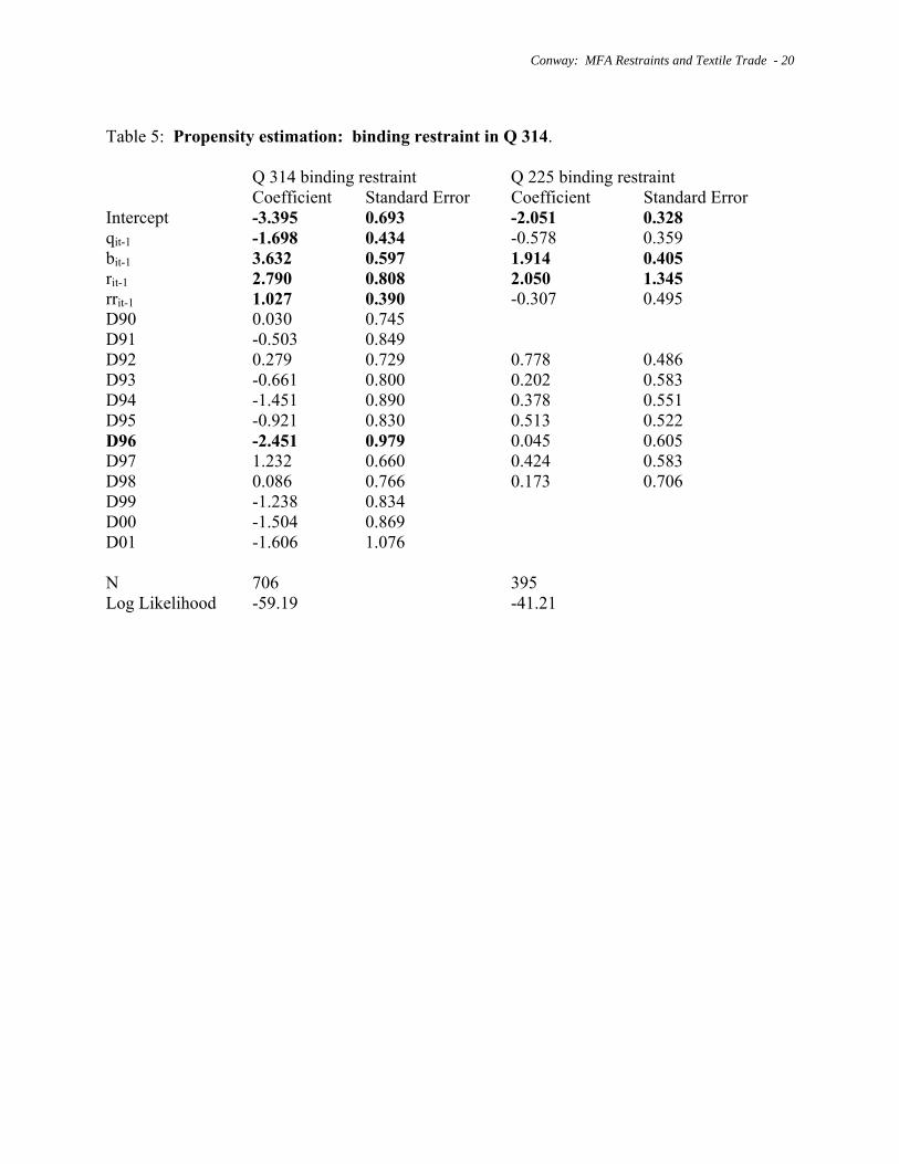
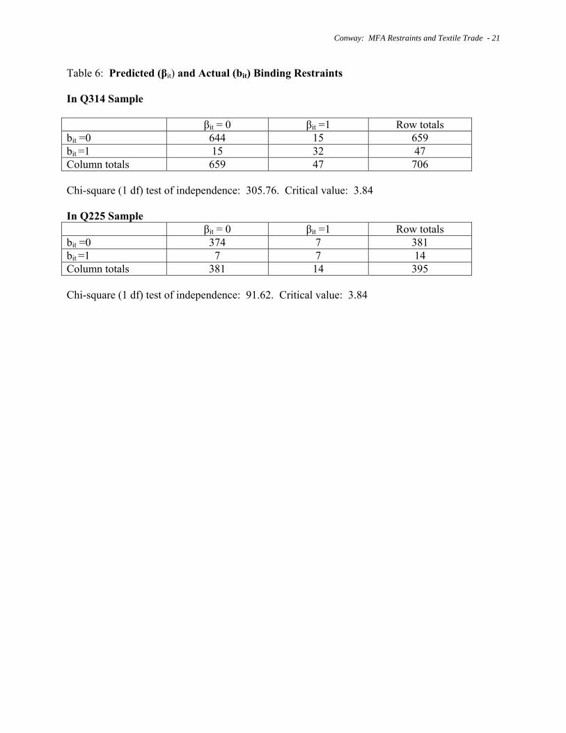
jt, and the Lagrangean multiplier λjt for binding restraints. In the estimation results that follow I will first use a propensity-score technique to instrument for binding restraints and will then estimate jointly the remaining two-equation system. V. Estimation results Estimation for Q 314 begins with the propensity score for a binding restraint. A fill rate of greater than 0.90 is used as an indication of a binding restraint, as elsewhere in the literature. Table 5 reports the results from estimating the propensity score. Probability of binding restraint: Q 314. There were 47 observations of binding restraint during the period 1990-2002, and 660 observations of non-binding restraints, for the 39 countries with complete data for at least a portion of that 13-year period. Estimation of the propensity score controls for a number of variables observed in the previous period: the unit value of exports to the US (qit-1), whether the restraint was binding in the previous period (bit-1), whether the country was a recipient of direct spillovers from countries with binding restraints (rit-1), and whether a country was subject to binding restraint in a group that subsumes the category Q 314 (rrit-1).14 There are also year-specific dummy variables added to capture any demand-side variation in the market for broadwoven cotton cloth. The coefficients all take expected signs, and all but the coefficients on time-specific dummies are significantly different from zero.15 As the unit value of exports rises, the country is less likely to face binding restraint. A country under binding restraint in the previous period is more likely to face binding restraint in this period. The potential for spillovers does indeed raise the likelihood that a given country will face binding restraint. Also, a country facing a binding group restraint in period t-1 is other things equal more likely to face a binding Q 314 restraint in period t: this effect is independent of, and in addition to, the effect of binding past Q 314 restraint in the coefficient on bit-1. Of the time-specific variables, only the 1996 dummy variable is significant. It is negative, indicating that in that year the average country was less likely to face binding restraint, other things equal, than in 2002. The predicted value from this equation is known as the propensity score (pit). If I set pit > .40 as the cutoff for predicting a binding restraint, the resulting pattern of prediction is defined as the binary variable βit reported in Table 6. Of the 706 observations, 47 are of actual binding restraint. The model predicts a binding restraint correctly in (32/47) = 68

14 The spillover variable is defined as rjt = (1-bjt)*cbt, with cbt a measure of the cumulative share of imports in Q 314 coming from countries with binding restraints. This variable will be zero for a country under binding restraint, and will be equal to the share of imports coming from restrained countries otherwise. As this variable rises, spillovers to non-restrained countries are expected to rise. 15 In this and what follows, significance will be defined as “significant at the 95 percent level of confidence”.


percent of the cases, and a non-binding restraint correctly in (644/659) = 98 percent of the cases. In all, the percent of observations predicted correctly is over 95 percent. . Market determination: Q 314. The joint estimation of (5) and (10) yields the coefficients reported in Tables 7 and 8. The unit value q*

jt, the share of imports sjt and the probability of being in a binding restraint are treated as jointly determined. The first three columns of each table report the error-correction version of the model, while the final three columns report the model as estimated in terms of levels. In each group of three columns, the first represents a specification controlling both for country-specific and for time-specific factors. The second is the specification with time-specific factors, while the third includes only the variables listed in the first column.16 The three specifications yield similar interpretations, so consider the coefficients of the first column in Tables 7 and 8. The first column of Table 7 illustrates that the share of imports in this category from country j follows an error-correction process, with both lagged difference and lagged share term having significant negative coefficients. The market share also responds significantly and negatively as expected to real exchange rate appreciation. The four regressors associated with the quota program are largely insignificant. Countries that have negotiated quotas in place (binding or not) are insignificantly different from those without quotas in the growth of import share. Those with binding restraint are insignificantly different from all others in the growth of market share (although when country-specific effects are not included (columns two and three) the countries with binding restraints have significantly faster growth in market share). There is a positive spillover effect, with those countries without binding restraints benefiting from increased market share as the proportion of imports from countries with binding restraints increases. Binding secondary (or group-level) restraints have an insignificant effect on growth in market share as well. The coefficient on unit value is negative, as expected, but insignificantly different from zero. Unit values also show evidence of following an error-correction process, but beyond that little is significant. The impact of the restraint program on unit value is negative, contrary to prediction, but insignificant. (When country-specific effects are excluded, the coefficients on pjt and βjt are both negative and significant. This is probably due to unobserved country-specific effects: Indonesia, for example, is both a low-cost producer and a country governed by restraints.) Spillover effects are negative, but insignificant; group-level binding restraints put upward pressure on the unit values, other things equal. Propensity to binding restraint: Q 225. I follow the same estimation strategy for Q 225. There are 29 countries for which there are non-zero exports to the US in this category and for which there are sufficient data to conduct the estimation. There are 14 instances of binding specific restraints in the sample. These only occur in 1991-1998, and so the propensity-score estimation includes only those time-specific variables. The 16 The coefficients of the time-specific and country-specific variables are not reported, but are available on request.


coefficients for that estimation are reported in Table 5, and are quite similar to those of Q 314. The propensity to have a binding restraint predicts the observed outcome fairly well. It matches only 7 of the 14 binding restraints, but 374 of the 381 non-binding observations. On average, it predicts correctly, once again, over 95 percent of the total. Tables 9 and 10 report the joint estimates of the equations (5) and (10). Focus for the moment on the coefficients in columns 1. In Table 9, it is clear that blue denim import shares follow an error-correction process similar to that of broadwoven cotton. The real-exchange-rate effect is once again negative, but insignificantly so, as is the price impact on demand. Of the four quota-related variables, two are significant in determining import shares: those countries participating in negotiated restraints are significantly more likely to have growing market share. Binding specific quotas have a positive, but insignificant, effect on share growth, while binding group-level quotas have a significant negative effect on import growth.17

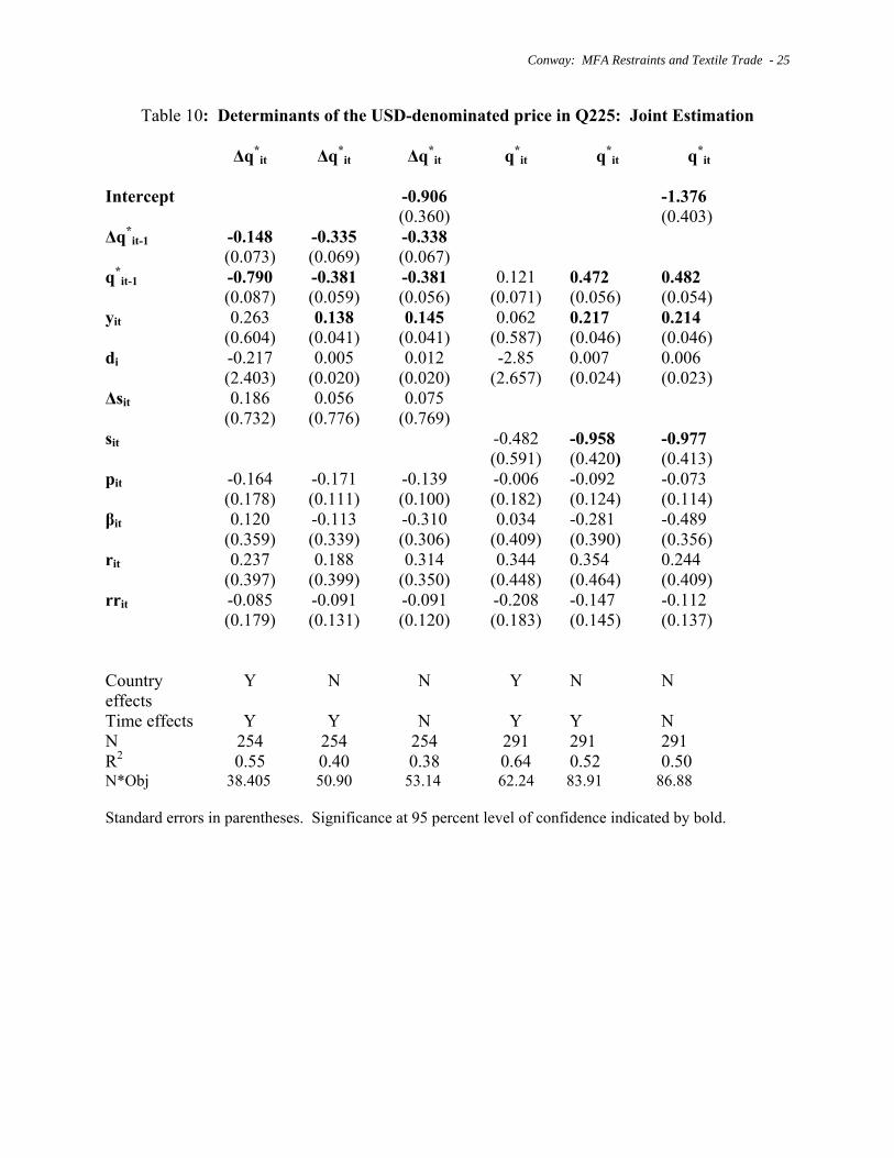
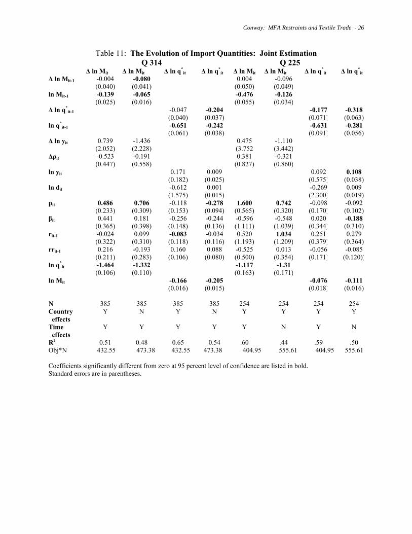
In Table 10, the evolution of unit values appears to have no significant relation to the restraint system. There is a more negative trend in unit values among those countries participating in negotiated restraints, and somewhat higher unit values among those with binding specific restraints. Secondary binding restraints have the effect of depressing unit value growth, while the spillover effect of binding quotas in other countries is positive, as expected. All of these effects are insignificantly different from zero, though, in all specifications. Reconsidering, using quantities. While the preceding calculations were undertaken based upon the import share equations, the negotiated restraints are based in terms of growth rates of physical quantities of imports. As such, a binding restraint may have no measurable impact on the shares of imports while being a constraint on quantities imported into the US. To examine this, the analysis of the preceding sections is redone using a market system of unit values and quantities imported: the results are reported in Table 11. The results for Q 314 are reported in the first four columns, and those for Q 225 in the final four columns. For each category, the results are reported including country-specific and time-specific effects (odd columns) and time-specific effects only (even columns). The price elasticities of demand are reported in the ln q*

jt row, while the supply elasticities of import pricing are given in the ln Mjt row. The estimates suggest a quite reasonable price elasticity of demand of between -1.11 and -1.46 in these two categories, while the pricing equation suggests that to increase a single country’s exports to the US by one hundred percent the price of the imported cloth from that country must fall by between 7.6 and 16.6 percent. These estimates stand in sharp contrast to those of Panagariya et al. (2002) and suggest that the assumption that the quota system ensures a fixed quantity of exports is extreme.

17 The positive effect of binding specific restraints is reversed, but still insignificant, if country-specific effects are excluded.


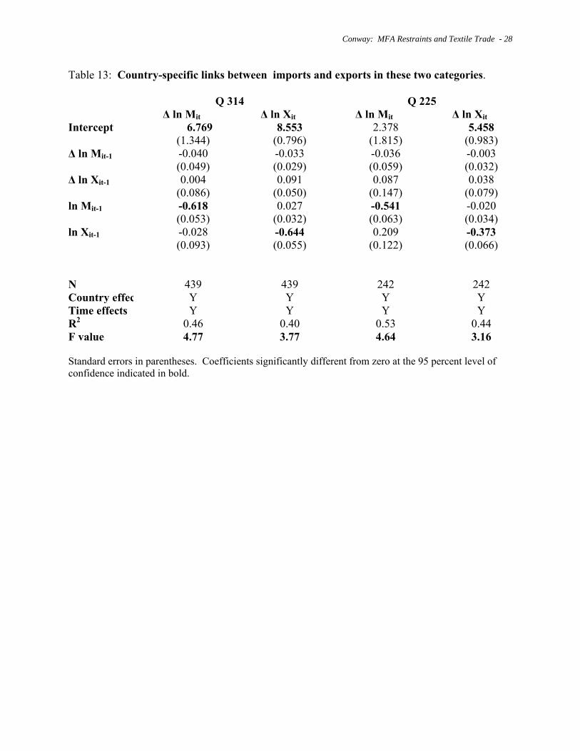
Average tendencies in imports and exports. The preceding analysis has been undertaken in terms of country shares in total imports or by country quantities. It is also useful to examine the aggregate tendencies in imports and exports for the two restraint categories. In the following I stack the aggregate measures of quantities traded for the years 1990-2002 with the goal of uncovering the aggregate dynamics of imports and exports over this period. Table 12 reports the aggregate dynamic of imports and exports if the coefficients in the two categories are assumed to be identical.18 In the first column, the aggregate imports into the US follow a simple error-correction model: aggregate imports grow at a 3.84 percent, and the economy makes up 30.8 percent of any deviations from long-run import quantity in the following year.19 There is no significant acceleration in import growth over time. Exports grow at a very similar 3.70 percent rate per year, and the economy makes up 36 percent of any deviation from long-run exports in the year following the shock. There is also a significant relative-price effect: as the price of imports rises by one percent relative to the price of exports (as measured by unit values), the quantity exported grows by 13 percent in aggregate. There is also an increase in aggregate export quantity growth over time, as indicated by the significant time trend. Table 13 reports an investigation in country-specific links between export and import quantities. As is evident there (and in Table 12 for the aggregate), exports and imports are independent activities: increasing exports to our trading partners do not encourage imports in that same category in subsequent years, and increasing imports from our trading partners do not encourage exports from the US in subsequent years. There is an insignificant positive effect of export growth in period t-1 on export growth in period t, suggesting a dynamic divergence in supply to those countries; by contrast, there is an insignificant negative effect of former import growth on current import growth, suggesting a diversification of imports among an increasing number of importers. Figures 11 and 12 plot the year-specific effects associated with the regressions in Table 13. In Figure 11 the year-specific movements in Q 225 imports and exports are plotted: imports were more volatile than exports prior to 1995 (in large part because they were larger in magnitude). Post-1995, the imports and exports tended to move counter to one another, in part perhaps because of real-exchange-rate movements but also because of world shocks (e.g., the Asian crisis). VI. Conclusions. This research is in its early stages; more sophisticated modeling and consideration of more quota categories will be useful in making these results more precise. I draw a number of initial conclusions from this research to date:

18 This is an undesirable assumption, but one necessary to have larger number of observations for statistical testing. 19 Time-specific effects, and separately a “denim” effect giving a separate intercept for category 225, were introduced but had coefficients insignificantly different from zer0.


o The Q 225 and Q 314 categories of trade restraint include trade with a broad spectrum of countries, only a few of which are subject to the negotiated restraints of the ATC.

o There is substantial intra-industry trade in these categories, with exports

exceeding imports in both categories by 2002. This aggregate intra-industry trade does not for the most part correspond to country-specific intra-industry trade – the US tends to export from the Asian countries and to export to the Caribbean and NAFTA countries.

o There is no evidence that the quota system was effective in restraining

imports in aggregate into the US. While estimated coefficients take the sign suggested by theory, they are not significantly different from zero.

o When evaluating this restraint system, it is important to consider both

specific restraints and group restraints. In some cases, the group restraints are the ones found to have a significant effect in restricting trade.

o While there is suggestive evidence that imports are re-exported, the notion

of a specific link between exports and imports, both in aggregate and at the country level, is rejected. Further work will be necessary to confirm that this is not happening at a regional level (e.g., from Asian importers to exporters to the Caribbean).

The most obvious extension to be pursued is the consideration of other categories of imports under quota. It is also important to recognize what this exercise did not do. Much of the current concern about removal of restraints focuses upon the capacity of a single country, China, to supply the world market in these categories. The econometric analysis of the previous sections treated China as only one of many countries, and thus reduced the relative weight of that threat in the overall market. It will be useful in future research to address explicitly the Chinese presence across quota categories to identify more precisely the contribution that China can potentially play across these markets.


Table 1: Quota Agreements under the ATC Country type of quota Growth Swing/shift Q 225: Blue Denim Fabric Malaysia specific limit 11.049 7.00 Egypt specific limit 12.702 6.00 Brazil specific limit 11.049 6.00 Macao specific limit 8.064 7.00 Indonesia specific limit 11.049 7.00 China specific limit 3.221 5.00 Hong Kong 218/225/317/326 2.762 6.00 Taiwan 225/317/326 3.175 7.00 India Group II 12.89 15.00 Korea Group I 2.210 3.80 Philippines Group II 16.574 7.00 Q 314: Broadwoven Fabric/Poplin Malaysia specific limit 11.049 7.00 Brazil specific limit 11.049 6.00 Macao specific limit 8.064 7.00 China specific limit 3.221 5.00 Hong Kong specific limit 4.604 6.00 Taiwan specific limit 3.175 7.00 India specific limit 11.049 7.00 Korea specific limit 4.604 3.80 Pakistan specific limit 12.890 7.00 Sri Lanka specific limit 11.049 7.00 Romania specific limit 12.097 7.00 Philippines Group II 16.574 7.00 Egypt 314-O 12.702 6.00 Indonesia 314-O 11.049 7.00 Thailand 314-O 11.049 7.00 Turkey 314-O 11.049 7.00 Source: Summary of Agreements, OTEXA, 24 January 2003

Table 2: US Trade in Quota Category 314 with Three Trading Blocs

Mexico and Canada

CBI nations

Asian Exporters

Xq

Xv

Mq

Mv

Xq

Xv

Mq

Mv

Xq

Xv

Mq

Mv

1989 0.20 0.21 0.01 0.01 0.17 0.14 0.00 0.01 0.01 0.02 0.57 0.381990 0.26 0.24 0.02 0.02 0.17 0.14 0.00 0.00 0.02 0.02 0.62 0.451991 0.28 0.25 0.01 0.01 0.12 0.10 0.00 0.01 0.01 0.01 0.68 0.501992 0.32 0.28 0.00 0.00 0.09 0.09 0.00 0.00 0.04 0.02 0.66 0.531993 0.32 0.26 0.01 0.01 0.11 0.09 0.01 0.01 0.02 0.02 0.64 0.511994 0.33 0.27 0.01 0.01 0.09 0.09 0.01 0.02 0.01 0.02 0.76 0.571995 0.27 0.27 0.01 0.01 0.17 0.17 0.00 0.00 0.03 0.02 0.76 0.591996 0.31 0.29 0.01 0.01 0.26 0.27 0.00 0.01 0.02 0.01 0.83 0.641997 0.32 0.28 0.01 0.01 0.33 0.36 0.00 0.00 0.01 0.01 0.86 0.711998 0.28 0.28 0.01 0.01 0.42 0.41 0.00 0.00 0.01 0.02 0.86 0.711999 0.63 0.63 0.01 0.01 0.14 0.17 0.00 0.00 0.01 0.01 0.82 0.602000 0.58 0.57 0.01 0.01 0.19 0.21 0.00 0.00 0.01 0.01 0.81 0.642001 0.29 0.28 0.01 0.01 0.53 0.56 0.00 0.00 0.01 0.01 0.79 0.662002

0.27

0.25

0.01

0.01

0.60

0.63

0.00

0.00

0.01

0.01

0.72

0.62

NAFTA nations: Mexico and Canada CBI nations: Dominican Republic, Guatemala, Honduras, El Salvador, Haiti, Nicaragua and Costa Rica Asian exporters: Thailand, India, Pakistan, Indonesia, China and Malaysia Xq – export quantity (m2), Xv – export value (USD), Mq – import quantity (m2), Mv – import value (USD) Source: US International Trade Commission


Table 3: US Trade in Quota Category 225 with Three Trading Blocs

NAFTA countries

CBI nations

Asian exporters Xq Xv

Mq Mv Xq Xv Mq Mv Xq Xv Mq Mv

1989 0.37 0.40 0.03 0.03 0.02 0.02 0.00 0.00 0.08 0.07 0.74 0.741990 0.39 0.42 0.01 0.01 0.01 0.02 0.00 0.00 0.22 0.14 0.89 0.891991 0.38 0.41 0.03 0.04 0.02 0.02 0.00 0.00 0.18 0.15 0.91 0.891992 0.44 0.47 0.07 0.10 0.02 0.03 0.00 0.00 0.06 0.05 0.61 0.581993 0.48 0.47 0.08 0.12 0.02 0.03 0.00 0.00 0.05 0.06 0.65 0.581994 0.56 0.55 0.12 0.18 0.01 0.02 0.00 0.00 0.06 0.06 0.66 0.601995 0.47 0.46 0.18 0.24 0.04 0.04 0.00 0.00 0.07 0.07 0.59 0.531996 0.54 0.50 0.40 0.45 0.02 0.02 0.00 0.00 0.07 0.07 0.44 0.381997 0.50 0.49 0.58 0.63 0.04 0.04 0.00 0.00 0.04 0.04 0.31 0.261998 0.60 0.59 0.54 0.60 0.03 0.03 0.00 0.00 0.02 0.02 0.37 0.311999 0.76 0.76 0.55 0.59 0.02 0.02 0.00 0.00 0.02 0.02 0.34 0.292000 0.78 0.77 0.44 0.46 0.03 0.02 0.00 0.00 0.01 0.02 0.45 0.412001 0.76 0.75 0.36 0.35 0.07 0.07 0.00 0.00 0.01 0.02 0.55 0.532002

0.79

0.78

0.39

0.38

0.08

0.08

0.00

0.00

0.02

0.03

0.52

0.48

NAFTA countries: Mexico and Canada CBI nations: Dominican Republic, Guatemala, Honduras, El Salvador, Haiti, Nicaragua and Costa Rica Asian exporters: Thailand, India, Pakistan, Indonesia, China, Malaysia, Hong Kong and Taiwan Xq – export quantity (m2), Xv – export value (USD), Mq – import quantity (m2), Mv – import value (USD), Xq – export quantity (m2)


Table 4: Share of Trading Blocs in Total US Trade in Q314 and Q225 Q 314 groups Q 225 groups Xq Xv Mq Mv Xq Xv Mq Mv

1989 0.57 0.52 0.67 0.64 0.47 0.49 0.77 0.78 1990 0.58 0.53 0.68 0.65 0.62 0.58 0.90 0.90 1991 0.54 0.49 0.76 0.71 0.58 0.58 0.93 0.93 1992 0.56 0.50 0.74 0.73 0.52 0.56 0.68 0.69 1993 0.54 0.45 0.73 0.74 0.56 0.56 0.73 0.70 1994 0.53 0.47 0.84 0.81 0.63 0.62 0.78 0.78 1995 0.56 0.54 0.82 0.79 0.58 0.57 0.77 0.76 1996 0.63 0.62 0.91 0.87 0.63 0.59 0.83 0.83 1997 0.70 0.69 0.90 0.87 0.58 0.57 0.88 0.89 1998 0.76 0.75 0.90 0.83 0.65 0.65 0.91 0.91 1999 0.82 0.85 0.87 0.74 0.80 0.80 0.88 0.88 2000 0.82 0.83 0.85 0.80 0.81 0.81 0.89 0.87 2001 0.85 0.88 0.83 0.80 0.84 0.83 0.91 0.88 2002 0.88 0.90 0.76 0.77 0.88 0.88 0.91 0.86


Table 5: Propensity estimation: binding restraint in Q 314. Q 314 binding restraint Q 225 binding restraint Coefficient Standard Error Coefficient Standard Error Intercept -3.395 0.693 -2.051 0.328 qit-1 -1.698 0.434 -0.578 0.359 bit-1 3.632 0.597 1.914 0.405 rit-1 2.790 0.808 2.050 1.345 rrit-1 1.027 0.390 -0.307 0.495 D90 0.030 0.745 D91 -0.503 0.849 D92 0.279 0.729 0.778 0.486 D93 -0.661 0.800 0.202 0.583 D94 -1.451 0.890 0.378 0.551 D95 -0.921 0.830 0.513 0.522 D96 -2.451 0.979 0.045 0.605 D97 1.232 0.660 0.424 0.583 D98 0.086 0.766 0.173 0.706 D99 -1.238 0.834 D00 -1.504 0.869 D01 -1.606 1.076 N 706 395 Log Likelihood -59.19 -41.21


Table 6: Predicted (βit) and Actual (bit) Binding Restraints In Q314 Sample βit = 0 βit =1 Row totals bit =0 644 15 659 bit =1 15 32 47 Column totals 659 47 706 Chi-square (1 df) test of independence: 305.76. Critical value: 3.84 In Q225 Sample βit = 0 βit =1 Row totals bit =0 374 7 381 bit =1 7 7 14 Column totals 381 14 395 Chi-square (1 df) test of independence: 91.62. Critical value: 3.84


Table 7: The Evolution of Import Shares in Q314: Joint Estimation ∆sit ∆sit ∆sit sit sit sitIntercept 0.000 0.002 (0.001) (0.009)∆sit-1 -0.264 -0.403 -0.398 (0.048) (0.040) (0.044) sit-1 -0.326 -0.033 -0.033 0.542 0.939 0.939 (0.046) (0.018) (0.018) (0.042) (0.020) (0.020)∆yit -0.001 -0.009 -0.008 (0.026) (0.026) (0.025) ∆ρit -0.012 -0.013 -0.012 (0.006) (0.006) (0.006) yit

0.000 -0.000 -0.000 (0.000) (0.001) (0.001) (0.189) (0.004) (0.003)ρit

-0.002 0.002 0.002 (0.002) (0.005) (0.005)pit -0.002 -0.003 -0.003 -0.002 -0.002 -0.002 (0.004) (0.003) (0.003) (0.004) (0.004) (0.004)βit 0.010 0.018 0.016 0.005 0.012 0.012 (0.005) (0.005) (0.005) (0.006) (0.006) (0.006)rit-1 0.009 0.006 0.004 0.009 0.004 0.004 0.004 (0.004) (0.004) (0.004) (0.004) (0.005)rrit-1 0.001 -0.002 -0.002 -0.003 -0.002 -0.002 (0.003) (0.003) (0.003) (0.004) (0.003) (0.003)q*

it -0.001 -0.001 -0.001 -0.002 -0.001 -0.001 (0.001) (0.001) (0.001) (0.002) (0.001) (0.001) N 421 421 421 423 423 423 Country effect Y N N Y N N Time effects Y Y N Y Y N R2 0.34 0.20 0.20 0.94 0.93 0.93Obj*N 69.65 113.40 117.65 69.95 112.53 116.70 Coefficients significantly different from zero at 95 percent level of confidence are listed in bold. Standard errors are in parentheses.


Table 8: Determinants of the USD-denominated price in Q314: Joint Estimation

∆q*it ∆q*

it ∆q*it q*

it q*it q*

it Intercept 0.290 -0.365 (0.274) (0.280) ∆q*

it-1 -0.020 -0.224 -0.232 (0.046) (0.045) (0.044) q*

it-1 -0.879 -0.369 -0.366 0.065 0.462 0.458 (0.066) (0.046) (0.045) (0.044) (0.039) (0.038) yit 0.222 0.017 0.015 0.262 0.106 -0.000 (0.211) (0.030) (0.030) (0.214) (0.031) (0.001) di -0.611 0.002 0.004 -0.511 0.035 -0.001 (1.822) (0.018) (0.018) (1.870) (0.020) (0.001) ∆sit -0.203 -1.210 -1.253 (1.250) (1.388) (1.380) sit -2.136 -1.630 -1.567 (1.244) (0.623) (0.621) pit -0.277 -0.457 -0.457 -0.298 -0.384 -0.404 (0.176) (0.115) (0.107) (0.175) (0.121) (0.116) βit -0.330 -0.345 -0.351 -0.328 -0.265 -0.246 (0.172) (0.168) (0.152) (0.177) (0.194) (0.178) rit -0.145 -0.042 -0.009 -0.148 -0.144 -0.073 (0.138) (0.145) (0.128) (0.139) (0.158) (0.143) rrit 0.222 0.086 0.076 0.195 0.035 0.006 (0.123) (0.100) (0.094) (0.122) (0.106) (0.101) Country effects

Y N Y Y N N

Time effects Y Y Y Y Y N N 428 428 428 423 423 423 R2 0.53 0.48 0.54 0.81 0.69 0.68 N*Obj 55.95 83.23 85.34 69.95 112.53 116.70 Standard errors in parentheses. Significance at 95 percent level of confidence indicated by bold.


Table 9: The Evolution of Import Shares in Q 225: Joint Estimation ∆sit ∆sit ∆sit sit sit sitIntercept 0.003 -0.007 (0.003) (0.026)∆sit-1 0.203 0.146 0.151 (0.050) (0.049) (0.048) sit-1 -0.332 -0.156 -0.142 0.734 0.877 0.877 (0.046) (0.027) (0.027) (0.040) (0.026) (0.026)∆yit 0.028 -0.046 -0.037 (0.103) (0.085) (0.083) ∆ρit -0.008 -0.002 -0.006 (0.023) (0.022) (0.021) yit

-0.080 0.001 0.001 (0.041) (0.003) (0.003)ρit

-0.042 -0.001 -0.001 (0.020) (0.013) (0.013)pit 0.035 0.027 0.021 0.020 0.015 0.015 (0.015) (0.007) (0.007) (0.012) (0.006) (0.007)βit 0.005 -0.031 -0.020 -0.004 -0.025 -0.025 (0.030) (0.026) (0.023) (0.029) (0.022) (0.022)rit-1 -0.038 -0.010 -0.007 -0.050 0.000 0.000 (0.032) (0.030) (0.026) (0.031) (0.025) (0.025)rrit-1 -0.033 -0.018 -0.013 -0.003 -0.010 -0.011 (0.014) (0.008) (0.003) (0.004) (0.007) (0.008)q*

it -0.001 -0.001 -0.001 -0.001 -0.002 -0.002 (0.004) (0.004) (0.004) (0.013) (0.003) (0.003) N 254 254 254 291 291 291 Country effect Y N N Y N N Time effects Y Y N Y Y N R2 0.26 0.15 0.12 0.87 0.85 0.85Obj*N 38.40 50.90 53.14 62.24 83.91 86.89 Coefficients significantly different from zero at 95 percent level of confidence are listed in bold. Standard errors are in parentheses.


Table 10: Determinants of the USD-denominated price in Q225: Joint Estimation

∆q*it ∆q*

it ∆q*it q*

it q*it q*

it Intercept -0.906 -1.376 (0.360) (0.403) ∆q*

it-1 -0.148 -0.335 -0.338 (0.073) (0.069) (0.067) q*

it-1 -0.790 -0.381 -0.381 0.121 0.472 0.482 (0.087) (0.059) (0.056) (0.071) (0.056) (0.054) yit 0.263 0.138 0.145 0.062 0.217 0.214 (0.604) (0.041) (0.041) (0.587) (0.046) (0.046) di -0.217 0.005 0.012 -2.85 0.007 0.006 (2.403) (0.020) (0.020) (2.657) (0.024) (0.023) ∆sit 0.186 0.056 0.075 (0.732) (0.776) (0.769) sit -0.482 -0.958 -0.977 (0.591) (0.420) (0.413) pit -0.164 -0.171 -0.139 -0.006 -0.092 -0.073 (0.178) (0.111) (0.100) (0.182) (0.124) (0.114) βit 0.120 -0.113 -0.310 0.034 -0.281 -0.489 (0.359) (0.339) (0.306) (0.409) (0.390) (0.356) rit 0.237 0.188 0.314 0.344 0.354 0.244 (0.397) (0.399) (0.350) (0.448) (0.464) (0.409) rrit -0.085 -0.091 -0.091 -0.208 -0.147 -0.112 (0.179) (0.131) (0.120) (0.183) (0.145) (0.137) Country effects

Y N N Y N N

Time effects Y Y N Y Y N N 254 254 254 291 291 291 R2 0.55 0.40 0.38 0.64 0.52 0.50 N*Obj 38.405 50.90 53.14 62.24 83.91 86.88 Standard errors in parentheses. Significance at 95 percent level of confidence indicated by bold.


Table 11: The Evolution of Import Quantities: Joint Estimation Q 314 Q 225 ∆ ln Mit ∆ ln Mit ∆ ln q*

it ∆ ln q*it ∆ ln Mit ∆ ln Mit ∆ ln q*

it ∆ ln q*it

∆ ln Mit-1 -0.004 -0.080 0.004 -0.096 (0.040) (0.041) (0.050) (0.049) ln Mit-1 -0.139 -0.065 -0.476 -0.126 (0.025) (0.016) (0.055) (0.034) ∆ ln q*

it-1 -0.047 -0.204 -0.177 -0.318 (0.040) (0.037) (0.071) (0.063)ln q*

it-1 -0.651 -0.242 -0.631 -0.281 (0.061) (0.038) (0.091) (0.056)∆ ln yit 0.739 -1.436 0.475 -1.110 (2.052) (2.228) (3.752 (3.442) ∆ρit -0.523 -0.191 0.381 -0.321 (0.447) (0.558) (0.827) (0.860) ln yit

0.171 0.009 0.092 0.108 (0.182) (0.025) (0.575) (0.038)ln dit

-0.612 0.001 -0.269 0.009 (1.575) (0.015) (2.300) (0.019)pit 0.486 0.706 -0.118 -0.278 1.600 0.742 -0.098 -0.092 (0.233) (0.309) (0.153) (0.094) (0.565) (0.320) (0.170) (0.102)βit 0.441 0.181 -0.256 -0.244 -0.596 -0.548 0.020 -0.188 (0.365) (0.398) (0.148) (0.136) (1.111) (1.039) (0.344) (0.310)rit-1 -0.024 0.099 -0.083 -0.034 0.520 1.034 0.251 0.279 (0.322) (0.310) (0.118) (0.116) (1.193) (1.209) (0.379) (0.364)rrit-1 0.216 -0.193 0.160 0.088 -0.525 0.013 -0.056 -0.085 (0.211) (0.283) (0.106) (0.080) (0.500) (0.354) (0.171) (0.120))ln q*

it -1.464 -1.332 -1.117 -1.31 (0.106) (0.110) (0.163) (0.171) ln Mit -0.166 -0.205 -0.076 -0.111 (0.016) (0.015) (0.018) (0.016) N 385 385 385 385 254 254 254 254 Country effects

Y N Y N Y Y Y Y

Time effects

Y Y Y Y Y N Y N

R2 0.51 0.48 0.65 0.54 .60 .44 .59 .50 Obj*N 432.55 473.38 432.55 473.38 404.95 555.61 404.95 555.61 Coefficients significantly different from zero at 95 percent level of confidence are listed in bold. Standard errors are in parentheses.


Table 12: Aggregate imports and exports in these two categories.

∆ ln Mt ∆ ln XtIntercept 3.837 3.704 (1.057) (1.246) ∆ ln Mt-1 0.016 -0.160 (0.172) (0.232) ∆ ln Xt-1 -0.213 -0.044 (0.142) (0.180) ∆ ln (qxt/qmt) 3.978 13.330 (4.113) (6.017) ∆ ln Qct 1.028 -2.187 (2.327) (2.992) ln Mt-1 -0.308 (0.092) ln Xt-1

-0.361

(0.126) t 0.094 (0.026) N 22 22 Country effect N N Time effects N N R2 0.49 0.49 F value 3.24 2.58 Standard errors in parentheses. Coefficients significantly different from zero at the 95 percent level of confidence indicated in bold.


Table 13: Country-specific links between imports and exports in these two categories. Q 314 Q 225 ∆ ln Mit ∆ ln Xit ∆ ln Mit ∆ ln XitIntercept 6.769 8.553 2.378 5.458 (1.344) (0.796) (1.815) (0.983) ∆ ln Mit-1 -0.040 -0.033 -0.036 -0.003 (0.049) (0.029) (0.059) (0.032) ∆ ln Xit-1 0.004 0.091 0.087 0.038 (0.086) (0.050) (0.147) (0.079) ln Mit-1 -0.618 0.027 -0.541 -0.020 (0.053) (0.032) (0.063) (0.034) ln Xit-1 -0.028 -0.644 0.209 -0.373 (0.093) (0.055) (0.122) (0.066) N 439 439 242 242 Country effec Y Y Y Y Time effects Y Y Y Y R2 0.46 0.40 0.53 0.44 F value 4.77 3.77 4.64 3.16 Standard errors in parentheses. Coefficients significantly different from zero at the 95 percent level of confidence indicated in bold.


Figure 1: Aggregate US Production and Trade, Q225

0

100

200

300

400

500

600

700

800

900

1988 1989 1990 1991 1992 1993 1994 1995 1996 1997 1998 1999 2000 2001 2002 2003

Mill

ions

of s

quar

e m

eter

s

Export 225 Import 225 Production 225 Sources: OTEXA, US Department of Commerce; US International Trade Commission

Figure 2: Aggregate US Production and Trade, Q314

0

50

100

150

200

250

300

1988 1989 1990 1991 1992 1993 1994 1995 1996 1997 1998 1999 2000 2001 2002

Mill

ions

of s

quar

e m

eter

s

US Production US Exports US Imports Sources: OTEXA, US Department of Commerce; US International Trade Commission


Figure 3: Two-way Trade in Textiles

0

0.5

1

1.5

2

2.5

3

3.5

4

4.5

1989 1990 1991 1992 1993 1994 1995 1996 1997 1998 1999 2000 2001 2002

Rat

io o

f Exp

ort V

alue

to Im

port

Val

ue

Q 314: Broadwoven Cotton

Q 225: Blue Denim

Source: US International Trade Commission (http://dataweb.usitc.gov)

Figure 4: Unit Values of Textiles Traded by the US

0.50

0.75

1.00

1.25

1.50

1.75

2.00

2.25

2.50

2.75

1989 1990 1991 1992 1993 1994 1995 1996 1997 1998 1999 2000 2001 2002

USD

per

squ

are

met

er

225 Export Value 225 Import Value 314 Export Value 314 Import Value Source: US International Trade Commission (htttp://dataweb.usitc.gov)


Figure 5: Evolution of Import Share, Q314

0

2.5

5

7.5

10

12.5

15

17.5

20

22.5

25

0 2.5 5 7.5 10 12.5 15 17.5 20 22.5 25

Import Share 1996

Impo

rt S

hare

198

9

Indonesia

Thailand

Malaysia

China

Japan

Korea

Italy

India

Taiwan

France

Source: US International Trade Commission

Figure 6: Evolution of Import Share, Q314

0

2.5

5

7.5

10

12.5

15

17.5

20

22.5

25

0 2.5 5 7.5 10 12.5 15 17.5 20 22.5 25

Import Share 2001

Impo

rt S

hare

199

6

China

Indonesia

Thailand

Japan

UAE

Korea

Pakistan

IndiaItaly

Bahrain

Malaysia

Taiwan

France

Portugal



Figure 7: Evolution of Import Shares, Q 225

0

5

10

15

20

25

30

35

40

45

50

0 5 10 15 20 25 30 35 40 45 50

Shares in 1996

Shar

es in

198

9

Taiwan

Hong Kong

Brazil

Argentina

MexicoCanada

Spain, India, UAE


Figure 8: Evolution of Import Shares, Q 225

0

5

10

15

20

25

30

35

0 5 10 15 20 25 30 35

Shares in 2001

Shar

es in

199

6

Taiwan

Hong Kong

Brazil

India

Mexico

Canada

Spain

IndonesiaItaly

Pakistan



Figure 9: Unit Values and Import Shares in 2001 for Q225

0

1

2

3

4

5

6

0 5 10 15 20 25 30 35

Share of US Imports in category Q225

Uni

t Val

ue o

f Im

port

s fr

om th

at C

ount

ry

MexicoHong KongTaiwan

Canada

Italy

Turkey

Japan

Indonesia

MalaysiaChina


Figure 10: Unit Value and Import Share in 2001 for Q314

0

1

2

3

4

5

0 5 10 15 20 25

Import Share

Uni

t Val

ue (U

SD p

er s

quar

e m

eter

)

Indonesia ChinaThailand

Japan

UAE

Korea

Pakistan

India

Italy

Bahrain, Malaysia

Taiwan

France

Portugal



Figure 11: Year-specific Effects in Q225 Imports and Exports

-2

-1.5

-1

-0.5

0

0.5

1

1.5

1989 1990 1991 1992 1993 1994 1995 1996 1997 1998 1999 2000 2001 2002

m225 x225 Source: US International Trade Commission, and Table 13

Figure 12: Year-specific Effects in Q314 Imports and Exports

-0.6

-0.4

-0.2

0

0.2

0.4

0.6

0.8

1989 1990 1991 1992 1993 1994 1995 1996 1997 1998 1999 2000 2001 2002

m314 x314 Source: US International Trade Commission, and Table 13


Bibliography. Abernathy, F., J. Dunlop, J. Hammond and D. Weil: A Stitch in Time. New York, NY:

Cambridge University Press, 1999. Cline, W.: The Future of World Trade in Textiles and Apparel. Washington, DC: Institute for

International Economics, 1987. Dean, J.: “The Effects of the US MFA on Small Exporters”, Review of Economics and Statistics

72/1, 1990, pp. 63-69. Dean, J.: “Market Disruption and the Incidence of VERs under the MFA”, Review of

Economics and Statistics 77/2, 1995, pp. 383-388. Evans, C. and J. Harrigan: “Distance, Time and Specialization”, Board of Governors

International Finance Discussion Papers 766, 2003. Panagariya, A., S. Shah and D. Mishra: “Demand Elasticities in International Trade: Are They

Really Low?”, Journal of Development Economics 64/2, 2001, pp. 313-342. Trela, I. and J. Whalley: “Global Effects of Developed-Country Trade Restrictions on Textiles

and Apparel”, Economic Journal 100, 1990, pp. 1190-1205. US International Trade Commission report 3519, “Economic Effects of Significant US Import

Restraints”, June 2002. Yang, Y., W. Martin and K. Yanagishima: “Evaluating the Benefits of Abolishing the MFA in

the Uruguay Round Package”, chapter 10 in Hertel, T., ed.: Global Trade Analysis. Cambridge, UK: Cambridge University Press, 1997.

Date post:	22-Apr-2018
Category:	Documents
Upload:	truongngoc
View:	222 times
Download:	3 times

Draft -- comments welcome. Please do not quote without...

Documents