DRAFT - In Review for Conservation Biology 16 March...

DRAFT - In Review for Conservation Biology 16 March 2007

Forks in the road: choices in GIS procedures for designing wildland linkages PAUL BEIER,* DANIEL R. MAJKA,* AND WAYNE D. SPENCER†

*School of Forestry and Merriam-Powell Center for Environmental Research, Northern Arizona University, Flagstaff, AZ 96011-5018 U.S.A.

†Conservation Biology Institute, 815 Madison Avenue, San Diego, CA 92116 U.S.A.

Abstract: GIS procedures are commonly used to identify lands that will best maintain the ability of wildlife to move between wildland blocks through matrix lands after the remaining matrix has become incompatible with wildlife movement. Unfortunately, many corridor and linkage designs based on GIS procedures lack transparency because key assumptions are unstated and alternative approaches are rarely mentioned or compared. We offer a roadmap of 16 choices and assumptions that arise in designing linkages to facilitate movement or gene flow of focal species between two or more pre-defined wildland blocks. We recommend that linkages be designed to serve multiple (rather than one) focal species likely to serve as a collective umbrella for all native species and ecological processes, explicit acknowledgment of untested assumptions, and the use of sensitivity analysis to present model uncertainty. Such uncertainty is best displayed to stakeholders as maps of modeled linkages under different assumptions. We also recommend modeling corridor dwellers (species that require more than one generation to move their genes between wildland blocks) differently from passage species (for which an individual can move between wildland blocks within a few weeks). We identify a problem (which we label the subjective translation problem) that arises because the analyst must subjectively decide how to translate measurements of resource selection into resistance (the difficulty with which a species can move through a pixel with specified attributes). This problem can be overcome by developing ways to estimate resistance from observations of genetic distances or interpatch movements. There is room for substantial improvement in procedures to design linkages robust to climate change, and in tools that allow stakeholders to compare an optimal linkage design to an alternative set of parcels meeting a cost constraint or other conservation goal.

Introduction

Habitat fragmentation is a major threat to wildlife populations and biodiversity (Wilcox & Murphy 1985; Wilcove et al. 1986; Fahrig & Merriam 1994), but wildland linkages or wildlife corridors can mitigate its negative effects (Beier & Noss 1998; Haddad et al. 2003). We define a corridor as a swath of land intended to allow passage by a particular wildlife species between two or more wildland areas. We use the term linkage to denote connective land intended to promote movement of multiple focal species or propagation of ecosystem processes; we also use linkage as a generic term when the distinction is unnecessary.

Designing a linkage involves identifying specific lands which – if conserved and integrated with underpasses or overpasses across potential barriers – will best maintain the ability of wildlife to move

between wildland blocks even after the remaining land (matrix) has been converted to uses incompatible with wildlife movement. GIS analyses, such as least cost analysis or spatially explicit population models, are at the heart of most science-based approaches to corridor and linkage design (but see Noss & Daly 2006 for “seat of the pants” approaches, and Fleury & Brown 1997 for an approach based on first principles of conservation biology). Approaches based on geographically explicit models are especially important when the potential linkage is not fully constrained by urbanization or other irreversible barriers, when the linkage is designed for multiple focal species, or when planners need to provide a transparent, rigorous rationale for a linkage design

Ironically, many linkage designs based on GIS procedures lack the transparency that should be a key advantage of a modeling approach. Key assumptions

1


are often unstated and the alternative approaches are rarely mentioned or compared. For example, in each of 21 recent papers using GIS procedures to design corridors or linkages (Table 1), the approach seemed reasonable but each approach was different. Perhaps each model was the best one for that particular landscape and focal species, but few modelers acknowledged other options or explored the sensitivity of the linkage design to alternatives.

Collectively, we have helped produce 25 linkage designs for landscapes in Arizona and southern California since 2001 (South Coast Wildlands 2003-2006; Beier et al. 2006, 2007). In our experience, stakeholder discomfort with a poorly defined or justified model can result in objections to the entire approach (Table 2). Conservation biologists should therefore structure and explain their analytical approaches and models in a way that addresses, or at least acknowledges, key assumptions and alternatives. Explicitly recognizing choices along the road to linkage design is essential to creating more rigorous and therefore more defensible conservation prescriptions.

In this paper, we offer an explicit roadmap of the assumptions and choices involved in designing linkages between two or more wildlands using GIS procedures and focal species. Thus we did not consider simulated annealing approaches (Andelman et al. 1999; Possingham et al. 2000) or spatially explicit population models (Carroll et al. 2003; Carroll 2006) that take a broader approach to reserve design, simultaneously prioritizing land both for core habitat blocks and linkages between them. Because conservation biologists often are faced with designing a linkage to connect two fixed reserve areas, our paper addresses a family of approaches appropriate in many landscapes.

We also concentrate on focal-species approaches, rather than approaches intended to promote general ecological connectivity (Hoctor et al. 2000; Carr et al. 2002; Marulli & Mallarach 2005) or to encompass environmental gradients or processes (Rouget et al. 2006). These latter approaches heavily weight naturalness of land cover, and may be more appropriate for depicting a coarse regional network than for designing a specific linkage. There is a lively debate on the relative merits of ecological indicators and focal species approaches in conservation (Brooks et al. 2004 and four responses in Conservation Biology 18), and scientists have only begun to explore how to design linkages for processes rather than species.

Developing our procedures (South Coast Wildlands 2003-2006, Beier et al. 2006, 2007) has been a tortuous journey, with many decision points, or forks, encountered along the road to linkage design. In some cases, we explored several paths before settling on one. At other forks, lack of time or data propelled us along a particular path, leaving us wondering how different the resultant linkage design would be at the end of a path not taken.

Our intent in this paper is to develop a framework for GIS-based linkage design that will facilitate sharing of lessons and reduce the risk that a practitioner will take a particular road fork without noticing alternative, and potentially better, options. We outline the choices facing the analyst, describe and evaluate some of the options at each decision point, and suggest how sensitivity analysis could inform these choices. Ultimately, we hope this framework will make linkage designs more defensible and successful.

THE BASIC ELEMENTS OF LINKAGE DESIGN

All published linkage designs based on focal species (Table 1) follow the same basic steps (Fig. 1). First the analyst defines the landscape of interest, selects one or more focal species, and develops an algorithm to estimate the resistance of each pixel for each species as a function of pixel attributes, such as land cover, topography, and level of human disturbance. Following Adriaensen et al. (2003), resistance refers to the difficulty of moving through a pixel, and cost (or effective distance) is the cumulative resistance incurred in moving from a pixel to both corridor terminuses. Next the analyst selects a swath of pixels with the lowest cost between wildlands; this swath is the corridor design or modeled corridor for one focal species. Corridor designs for multiple focal species are combined into a preliminary linkage design (Fig. 2), which becomes the final linkage design after it is modified to accommodate ecological processes, incorporate other pixels of conservation interest, buffer against edge effects, or achieve other objectives.

FORKS IN THE ROAD

Behind the straightforward façade of Figure 1 lie many choices that we present in an order corresponding to sequential analytic steps (Table 3).

How to define the analysis area?

The analysis area for a linkage design typically includes the wildland blocks to be linked, the matrix

2


between them, and some additional area to allow the model to identify looping corridors. Constraining the analytical window too much may exclude potential source patches, stepping-stone patches, or other facilitating elements that lie outside the core habitat blocks and intervening matrix, and thus may preclude optimal solutions (Adriaensen et al. 2003). On the other hand, if the goal is to identify a linkage across a particular landscape (e.g., between forests of Wyoming-Colorado and forests in Missouri-Arkansas, U.S.A.), it may be appropriate for the analysis area to exclude areas that may provide an alternative looping path (e.g., through the boreal forests of Canada). We believe all published linkage designs have appropriately disclosed and explained their decision to include or exclude important nearby areas.

Defining the wildland blocks (the large areas to be connected by a linkage design) is an important part of delineating the analysis area. Wildland blocks may be restricted to lands with the strongest conservation mandate (designated wilderness areas or strict nature reserves), or might be enlarged to include multiple use natural lands with various degrees of protection. As long as the areas to be connected are likely to remain wild for at least several decades, these blocks can be delineated on the basis of what conservation investors have an interest in protecting. However, the analyst should carefully consider this choice, as it will affect the map of the modeled linkage. Within a wildland block, habitat for each focal species may be limited in quality and amount, an issue we return to in How to delineate a corridor terminus and How to delineate habitat patches.

Which focal species?

Because large carnivores like bears and wolves live at low density and are among the first to be harmed by loss of connectivity, they are appropriate focal species for linkage design (Beier 1993; Servheen et al. 2001; Singleton et al. 2002). They also make popular flagships to increase stakeholder support for a linkage. Large carnivores were the only focal species in 9 of 20 linkage designs based on focal species (Table 1). However, we argue against designing a linkage solely for large carnivores – or any single species. Many other species need linkages to maintain genetic diversity and metapopulation stability. Furthermore most large carnivores are habitat generalists that can move through marginal and degraded habitats, and a corridor designed for them does not serve most habitat

specialists with limited mobility (Newell 2006). Indeed successful implementation of a single-species corridor for large carnivores could have a “negative umbrella effect” if land use planners and conservation investors become less receptive to subsequent proposals for less charismatic species. The umbrella effect of large carnivores best serves biodiversity if these species are part of a linkage designed for a broad array of native species.

We encourage the selection of focal species likely to collectively serve as an umbrella for all native species and ecological processes. For instance, Beier et al. (2006, 2007) invited agency, NGO, and academic biologists familiar with each linkage area to identify species with any of the following traits that would serve as umbrellas for other species sharing that trait: requiring dispersal between wildlands for metapopulation persistence, short or habitat-restricted dispersal movements, representative of an important ecological process (e.g., predation, pollination, fire regime), requiring connectivity to avoid genetic divergence of a now-continuous population, risk of change from being ecologically important to ecologically trivial if connectivity were lost, or reluctance to traverse barriers (e.g., culverts under roads). Each of their linkage designs had 10-20 focal species, often including reptiles, fish, amphibians, plants, and invertebrates.

If stakeholders are concerned that a linkage may increase the spread of invasive species into wildlands, then one or more invasive species should be included in the suite of focal species. Any expected invasion via the linkage should be compared to invasion expected from edges and matrix land regardless of the conserved linkage (see How to evaluate if the best is any good?)

Which landscape factors to include in the model?

Habitat use is driven by availability of food, nest sites, and other resources, safety from predators and other hazards, presence of competitors or facilitating species, and other factors (Guisan & Thuiller 2005). However these factors are rarely included in GIS models for linkage design, which are instead based on at most five factors, including land cover, one or two factors related to human disturbance, and one or two topographic factors (Table 1). These are chosen for the obvious reason that they are usually the only factors for which georeferenced data are available for the entire analysis area (Malczewski 2000). Because land cover is related to food and cover and humans are an important hazard

3


for many species, these GIS layers are related to ecologically important factors. However, to the extent that modeled factors are not comprehensive (fail to cover all aspects of the decision problem), GIS analysis can give misleading results (Malczewski 2000). We simply do not know how strongly the modeled layers are correlated with habitat use or movement by most focal species.

What can be done about insufficiency of factors? In the short term, linkage designers can start off with some simple honesty. Designers may have no choice but to build models based on factors for which data are available, even if the factors are not comprehensive, but credibility is strengthened by acknowledging the issue. In the long term, the scientific community can encourage development of GIS maps of soils1, rock outcrops, permanent water sources, and other factors known to affect habitat use by focal species. In our work in the southwestern USA, these factors are important for focal species such as pronghorn (Antilocapra americana), bighorn (Ovis canadensis), prairie dogs (Cynomys sp.), and many reptiles. With reliable GIS coverages of such features, we could immediately improve many models.

What metric for each factor?

Once factors are chosen, the analyst must next choose resistance-relevant metrics for each factor. Metrics can be categorical (land-cover types, topographic classes) or continuous (percent slope, distance from a cover type or road). Land-cover data are usually treated categorically, although meaningful continuous metrics can sometimes be derived to reflect, for example, tree-canopy closure or distance from forest or wetlands. Land-cover data may be available in a GIS layer with 20-30 coarse classes (National Land Cover Database in

1 Note to reviewers: In the US, the NRCS provides soil maps for most US counties (http://soils.usda.gov/ and http://soildatamart.nrcs.usda.gov/); their hi-resolution maps are SSURGO (their STATSGO maps are hopelessly coarse). However (a) the maps have big holes in them, (b) even within a single county they are NOT seamless: the map is a mosaic of polygons whose edges do not match, (c) you cannot make them seamless because the types of attributes recorded for polygons vary from one area to another even within a single county. Although good soil maps may exist in some agricultural counties, in many areas within the US they are NOT readily available and cannot be cobbled together from existing data. They are probably less available in most other countries.

the USA) or 70-100 classes (GAP data layers in the USA). Most wildlife habitat studies using these maps present the data as if they represented reality (Glenn & Ripple 2004), although classification accuracy is typically 60% to 80% (Yang et al. 2001); and digital maps developed from different remotely-sensed images produce markedly different depictions of vegetation (Glenn & Ripple 2004). We recommend that practitioners report resolution, accuracy, and source for land cover data.

In most linkage designs, human disturbance is measured by road density within a moving window around the focal pixel. Unfortunately, despite the seeming scale-invariance of length per length-squared, the calculated value of road density changes erratically and non-intuitively with the size of the moving window (D. R. Majka, in prep.). Thus, it is difficult to reliably estimate resistance for road density classes, and published estimates of animal occurrence with respect to road density cannot be translated to a different moving window size. Distance to nearest road avoids this problem, and may be a more appropriate road-related metric of human disturbance. Some models assign pixels containing a road a resistance value so high that the pixel is impermeable, or nearly so; Adriaensen et al. (2003) point out that the raster representation of roads in such models should be at least two pixels wide to avoid spurious gaps at pixel corners. However, we advise against assigning arbitrarily large resistance values to road-containing pixels, because bends in any given road will always create a raster representation with thinner areas that will be spuriously modeled as areas of lower resistance. Such distortion will have serious consequences when the model is used to identify locations for road-crossing structures.

GIS models can include one or more topographic metrics, such as elevation, aspect, insolation, slope, ruggedness, or topographic position, all of which are derived from a common set of digital elevation data. Some topographic metrics (e.g., elevation and aspect) probably affect animal movement by determining land cover or (for poikilotherms) by influencing the species’ thermal environment. Other topographic metrics such as ruggedness and topographic position may directly affect animal movements, adding new information to a model. Topographic position can be estimated by classifying pixels into any number of classes such as steep slope, ridgetop, or valley bottom; algorithms are provided by J. Jenness (http://www.jennessent.com/).

4

http://www.jennessent.com/

http://soils.usda.gov/

http://soildatamart.nrcs.usda.gov/


The algorithms for ruggedness and topographic position analyze pattern within a moving window, the size of which must be specified by the analyst. Although it is appealing to model topography from the perspective of the focal species, the scale at which most organisms assess topography is not known. More important, most cost values are assigned by making inferences from scientific publications, which usually report animal response to topography as it was perceived by the human researcher. Dickson and Beier (2007) illustrate the use of topographic position and discuss the issue of window size and other procedural decisions in this context. We encourage sensitivity analysis to address how these decisions affect a modeled corridor.

How to estimate resistance for each class of pixels?

Setting resistance values is “the link between the non-ecological GIS information and the ecological-behavioral aspects of the mobility of the organism or process” (Adriaensen et al. 2003:234). As such it has received more attention from linkage designers than any other decision discussed in this paper.

Resistance of each class of land use, topography, or human disturbance is usually based on expert opinion and literature review; Clevenger et al. (2002) emphasized the poor performance of expert opinion if not combined with literature review. In all published linkage designs, practitioners assigned scores on an arbitrary scale (typically 0 to 1, or 1 to 100). Because most of the relevant literature consists of studies of habitat use rather than animal movement, one end of the scale reflects the lowest possible resistance and best habitat quality, and the other end of the scale reflects highest resistance and worst habitat quality. In other words, one set of scores can be interpreted as both a resistance model and a habitat suitability model.

This complementarity between resistance and habitat suitability reflects the assumption that animals choose travel routes on the basis of the same factors they use to choose habitat. Although this seems reasonable, it may not always be true. For instance, Horskins et al. (2006) demonstrated that one corridor failed to provide gene flow for two species that occurred and probably bred within the corridor. Following Walker and Craighead (1997), we urge linkage designers to explicitly state this as a crucial assumption and acknowledge the extent to which the assumption is untested.

We introduce the term subjective translation to label an important problem that affects resistance estimates based on literature and expert opinion. Resource selection studies do not produce estimates of resistance, but instead produce a ranked list of land cover classes (or road density classes, topographic positions, etc.), a ratio or difference between use and availability of each class, number of animal occurrences in each class, or the mean distance from animal locations to the nearest occurrence of each class (Millspaugh & Marzluff 2001). Resistance could be related to these measures of resource selection in any number of ways (e.g., linear, concave, or convex functions). Few linkage analysts describe how they translate resource selection metrics into resistance, but even when they do (e.g., Ferreras 2001), the decision remains subjective.

Empirical data collected in the landscape of interest should provide a better basis than literature review for estimating resistance of various pixel classes. We consider four types of empirical data, in order of increasing relevance to functional connectivity:

• Species occurrence. Kobler & Adamic (1999), Ferreras (2001), Bani et al. (2002), and Adriaensen et al. (2007) estimated resistance of land use classes based on empirical data on occurrence or abundance of focal species in each land use class. Their approaches, and other approaches based on resource selection studies in the region of interest, improve on literature review or expert opinion by using animal observations in the linkage planning area, but are still affected by the subjective translation problem.

• Animal movement. Data on animal movements were used by Graham (2001) to assign resistance scores for Keel-billed Toucans (Ramphastos sulfuratus) and by Beier et al. (2007) to assign resistance scores for puma (Puma concolor). Movement data are more closely related to connectivity than presence or abundance, but this approach also suffers from the subjective translation problem.

• Rates of interpatch movement. If interpatch movement rates are a function of the resistance of each pixel type in the matrix between patches, multivariate methods can theoretically be used to identify the set of resistance values (a vector in matrix algebra) that best explains observed movement rates. Such estimates should be free of the subjective translation problem. However, Sutcliffe et al. (2003) noted two difficulties. First, unless the researcher samples the entire geographic range of the metapopulation, estimates will

5


be distorted due to (unmeasured) movements from patches outside the study area but within the interacting group of patches. Second, if the resistance vector includes 3 or more classes, it may be impossible to solve for a single best vector. Sutcliffe et al. (2003) addressed this problem by starting with a handful of likely vectors based on ecological knowledge of the focal species, and determining which of these vectors was most consistent with observed rates of interpatch movement. Similarly, Verbeylen et al. (2003) used an information theory approach to select which of 36 potential resistance vectors was most consistent with observed occupancy of putative sink patches. We encourage building on these two pioneering efforts by developing analytic routines that explore more of the potential vector space and efficiently search for an optimal solution. Both Sutcliffe et al. (2003) and Verbeylen et al. (2003) evaluated each vector based on the cost associated with a least-cost path between each pair of patches; such pixel-wide paths may poorly reflect the actual cost of interpatch travel. We recommend evaluating resistance vectors using tools that consider the cost of all possible interpatch paths, such as the isolation by resistance model (McRae 2006).

• Genetic distances among populations. Epps et al. (2005) used genetic analysis to estimate the resistance of highways to bighorn sheep movement by assigning each pixel of matrix to one of two resistance classes (one for the highway, one for all other matrix pixels). Gerlach and Musolf (2000) similarly estimated resistance of a river to movement of bank voles (Clethrionomys glareolus) using genetic distances and a binary map. This approach has the same advantages and problems as the approach using data on interpatch movements. Genetic data have the further advantage of reflecting only those interpatch movements that resulted in gene flow. However, genetic patterns reflect landscape pattern over an indeterminate number of generations, and are difficult to interpret when new roads or land uses have recently changed the landscape (Berry et al. 2005).

Despite these problems, we encourage development of resistance estimates based on genetic data or interpatch movements. Resistance estimates based on these data would have biological meaning, such that a 50% increase in resistance would correspond with a 50% decrease in movement. Because of the subjective translation problem, no such interpretation can be assigned to conventional resistance estimates. We

return to this issue in How to tell if the best is any good.

Several corridor and linkage designers conducted sensitivity analyses to assess the impact of the subjective translation problem (Quinby et al. 1999; Schadt et al. 2002; Larkin et al. 2004; Newell 2006; Adriaensen et al. 2007). Most of these papers suggest that the location of the modeled corridor does not change significantly as long as the rank order of resistance values is assumed correct. However, Schadt et al. (2002) attributed much of this insensitivity to the lack of alternative corridor locations in their highly urbanized potential linkage areas. In an extensive sensitivity analysis of the approach used by Beier et al. (2006), Newell (2006) found that modeled corridors were stable for five of eight focal species in a large (50 km long, 35 km wide) potential linkage area relatively unconstrained by existing urbanization.

Sensitivity analysis can estimate the impact of uncertainty only for a particular focal species and landscape. Perhaps after dozens of such analyses, we may have general rules about the types of species and landscapes that are insensitive to the subjective translation problem. Until then, we recommend that corridor designers routinely incorporate sensitivity analysis into their efforts. When sensitivity analysis suggests that a linkage design is sensitive to reasonable uncertainty in resistance estimates or other model elements, we further recommend that corridor designers present maps of model results under the most strongly divergent estimates of resistance, as Quinby et al. (1999) did.

How to combine factors?

To estimate the overall resistance of a pixel, the GIS analyst must combine resistance due to land cover with resistance due to human disturbance and other factors. To do so, the analyst must choose an arithmetic operation and assign a weight to each factor.

Most linkage designers used a weighted sum to combine factor resistances, but Singleton et al. (2002) used a weighted product and Beier et al. (2007) used a weighted geometric mean. The weighted product and geometric mean better reflect situations where one factor limits wildlife movement in a way that cannot be compensated by a lower resistance for another factor (US Fish & Wildlife Service 1981).

Regardless of arithmetic operation, each factor is assigned a weight reflecting its contribution to the overall resistance of a pixel. In all published linkage

6


designs, weights seem to have been assigned solely by expert opinion. The expert’s task is complicated by the fact that a factor’s weight reflects not only its importance, but also the factor’s range of variation and units of measurement (Malczewski 2000). Using a common scale (e.g., resistance units of 1 to 100) for each factor is common practice in least-cost modeling, and eliminates differences among factors in range and units of measurement. However, this pre-supposes that the resistance values for each factor were assigned in a way that compensates for differences among factors in range and units of measurement. Lacking evidence for this presupposition, we recommend that sensitivity analysis consider the simultaneous impact of uncertainty in both weights and class resistance scores, as was done by Quinby et al. (1999) and Newell (2006).

Although sensitivity analysis is a practical short-term solution, in the future we hope that empirical, multivariate resource selection studies will provide empirically-based weights and suggest the proper arithmetic procedure for combining factor resistances. Such empirical studies could also reveal important interactions between factors.

How to delineate a corridor terminus?

A terminus is that part of a wildland block that forms or “anchors” one end of a modeled corridor. A terminus can be defined as a point (pixel), a linear edge (e.g., the wildland boundary), or a patch (e.g., a patch of high-quality focal-species habitat within the wildland block). There can be more than one potential terminus in each wildland block.

Some linkage designs use each wildland block in its entirety as a terminus for each single-species analysis. However, in our experience this procedure sometimes produces a corridor that connects to a part of the wildland block far from any potential habitat for the focal species. This unreasonable result can be avoided by restricting terminuses to patches of known or potential breeding habitat (next section) within each wildland block.

Because distance is an important part of algorithms based on effective distance, in cases where two wildland blocks nearly touch at one or more locations, these algorithms tend to identify the narrowest gap as the best corridor, even if the modeled corridor is low in habitat value or movement potential. To avoid this problem, we recommend giving the GIS model “room

to run” by defining the terminuses well inside of the wildland blocks, perhaps as roughly parallel lines a few kilometers apart. Even if this modification does not change the modeled corridor for any focal species, it will demonstrate that the modeled corridor is not merely an artifact of boundary proximity.

Whether and how to delineate habitat patches?

Habitat patches are areas of habitat that can support reproduction by the focal species; they may occur within wildland blocks or matrix. Although linkage design does not require delineation of habitat patches, in our experience it is useful to delineate habitat patches as steppingstones within the matrix (next section), as terminuses within the wildland blocks (previous section), and as useful metrics for assessing functionality of a modeled linkage design (see How to evaluate if the best is any good?).

To delineate habitat patches, the analyst must specify a suitability threshold for habitat quality, the minimum area of suitable habitat necessary to sustain a breeding pair or population, and how non-habitat pixels (at patch edges or islets within a patch) affect habitat quality (e.g., via edge effects). South Coast Wildlands (2003-2006), Southern Rockies Ecosystem Project (2005), and Beier et al. (2007) illustrate procedures to identify pixels that are “good enough, big enough, and close enough together” to function as a habitat patch. To date, there has been no formal sensitivity analysis to determine how uncertainty in each of these three procedures affects either the map of habitat patches or the modeled corridor. Although we advocate for such sensitivity analysis, we believe the procedures currently in use provide reasonable patch maps, and that use of these maps is usually better than ignoring the distribution of breeding habitat in the planning area.

How to model corridor dwellers?

An unstated assumption in many corridor models is that an individual animal can move between wildland blocks in a single movement event of a few hours to a few weeks. Beier & Loe (1992) called such animals passage species, and pointed out that other focal species – corridor dwellers – require more than one generation to move their genes between wildland blocks. The distinction is based on an interaction between the species and the landscape, and thus a particular species could be a passage species if the habitat blocks are within dispersal distance, but a corridor dweller in another landscape with habitat

7


blocks more than one dispersal distance away. Corridor dwellers must find suitable breeding opportunities within the linkage.

To model movement by corridor dwellers, Wikramanayake et al. (2004), Beier et al (2007), and Adriaensen et al. (2007) assigned the lowest resistance value to habitat patches (previous section). We recommend this procedure when modeling a species with a few habitat patches imbedded in a matrix dominated by poor habitat. In such situations, the procedure tends to produce a corridor that links those patches in steppingstone fashion. However, if a large fraction of the matrix is near the threshold between suitable and unsuitable, a slight decrease in the threshold can cause most of the matrix to be mapped as a habitat patch, resulting in a highly linear corridor that fails to include the highest-quality habitat. In these situations, we discourage use of this procedure unless the analyst is confident that the threshold is precisely known.

The procedures of Wikramanayake et al. (2004) and Beier et al. (2007) could be improved by assigning the lowest resistance value only to potential breeding patches within effective dispersal distance of other potential breeding patches in the linkage. However, “effective dispersal distance” in this context means dispersal distance in suboptimal habitat, and such data are available for only a few species. Even if such data are available, it is not clear how to use such data (i.e., a frequency distribution of dispersal distances) to estimate the precise threshold at which interpatch connectivity is lost. A rigorous but data-hungry approach was suggested by van Langevelde (2000) who estimated this threshold distance from a time series of patch occupancy. Van Langevelde also illustrates how this threshold distance can then be used to estimate the effect of addition or deletion of candidate patches on the connectivity of a network of patches.

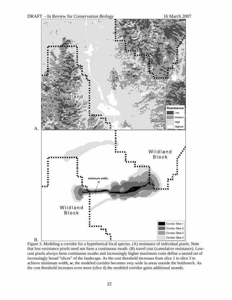
How to identify continuous swaths of low-resistance pixels?

Low resistance pixels may not form a continuous swath (Fig. 3). To identify well-connected low-resistance pixels, all published corridor designs (Table 1) calculated each pixel’s cost as the lowest possible cumulative resistance from that pixel to terminuses in each habitat block (Fig. 3). These cost values do form continuous swaths (modeled corridors).

Hargrove et al. (2004) present a promising

alternative based on individual-based movement models. Their approach simulates individual animals that leave each habitat block and explore the landscape using decision rules related to resistance of neighboring pixels until the individual either dies or reaches another habitat block. Pixels that are repeatedly chosen as part of successful paths are identified as part of the corridor. We encourage practical extension of these models to design corridors for species in real landscapes because they offer two advantages over conventional models. First, corridors identified by this approach are intuitively appealing because they consistently include patches of the best habitat in the matrix. This is also the only approach that does not assume that cost is symmetric (independent of the direction of travel), and thus could be used to assess the extent to which the optimal corridor in one direction coincides with the optimal corridor in the opposite direction. The volume of movement in some corridors is predominantly unidirectional due to funneling effect of the landscape configuration (Ferreras 2001) or asymmetric population sizes (Dixon et al. 2006). This raises the possibility that the location of a modeled corridor may also depend on direction of movement. The main drawback of individual-based movement models is that the user must specify values for several elusive parameters, such as probability of abrupt reversal of direction, energy costs of movement, likelihood of finding food, and likelihood of mortality in each type of habitat. Therefore, sensitivity analyses should be used to describe and illustrate sensitivity of the corridor to uncertainty in these parameters.

Graph theory (Bunn et al. 2000; Jordán 2000; Urban & Keitt 2001; Jordán et al. 2003; SREP 2005; Theobald 2006) and the isolation by resistance model (McRae 2006) may provide alternative ways to identify optimal paths. To date, these approaches have been limited to quantifying the effect of removing particular habitat patches from a landscape network, or descriptive measures of network connectivity, but in the future they may also be developed as tools for corridor and linkage design. The main hurdle arises because the goal of linkage design is to identify lands that will best maintain the ability of wildlife to move between wildland blocks even after the remaining land has been converted to uses incompatible with wildlife movement. Such land conversion profoundly affects the outputs of graph theory and isolation by resistance models, but has no effect on cumulative resistance, and probably little impact on the frequency with which pixels are used in

8


an individual-based movement model. Thus the main utility of these new approaches may be in linkage evaluation and empirical estimates of resistance, rather than linkage design.

How wide should a single-species corridor be?

A least-cost path is only one pixel wide; because such a narrow path could be identified within otherwise inappropriate habitat, it may be unlikely to be used and biologically irrelevant (Adriaensen et al. 2003). Furthermore, the location of a least cost path is highly sensitive to pixel size and errors in classifying single pixels (Broquet et al. 2006). Fortunately, the previous analytic steps produce a map in which increasingly wide corridors are displayed as nested polygons, each defined by the largest cost allowed in the polygon (Fig. 3B). As the cost threshold increases, multiple strands often emerge (e.g., swath 3 in Fig. 3B). Although a wider corridor is better in the sense that broad swaths include narrower ones, financial constraints favor smaller corridors. The analyst should present a graded cost map (e.g., Fig. 3B) to allow decision-makers to appreciate trade-offs. However, the decision-maker typically wants the analyst to present a preferred alternative, namely a corridor that is just wide enough to work. The width of the single-species corridor is most critical when a conservation plan is built for a single species, but even for multiple-species linkage designs, a stopping rule is needed to map each single-species corridor.

Harrison (1992) suggested that a corridor for a corridor dweller should be roughly the width of a focal species’ home range, or the square root of one-half of home range area (assuming home ranges approximate a 2:1 rectangle). However, if the focal species is strongly territorial, this could result in corridors fully occupied by home ranges where social interactions impede movement through the corridor (Horskins et al. 2006). Thus minimum corridor width for a corridor dweller should be substantially larger than a home range width.

A cost threshold that achieves a minimum width in a bottlenecked area will result in impractically broad swaths elsewhere (e.g. swath 4 in Fig. 3B). Therefore, corridor designers have used a variety of reasonable procedures to select an optimal or minimum corridor width. For example, Beier et al. (2007) specified a minimum width that had to be obtained in at least 90% of the corridor, but allowed a few short bottlenecks. Quinby et al. (1999) presented a series of potential corridors corresponding to various cost percentiles and

described the conservation implications of each option. Both approaches required iterative mapping and subjective evaluation. An objective set of decision rules, and an automated way to run them, would be significant advances. However, given myriad possible landscape configurations and reasonable differences of opinion about when a corridor is “big enough,” this may be an impossible goal.

How to combine corridors of multiple focal species?

The previous procedures produce a least-cost corridor for a single species. All 8 studies using multiple focal species (Table 1) presented separate maps for each focal taxon. Only Singleton et al. (2002), Beier et al. (2006, 2007), and Adriaensen et al. (2007) joined the single-species corridors into a multiple-species linkage design. Singleton et al. (2002) developed a “general carnivore model” by using the median resistance value for each pixel type across the 4 species modeled. We discourage this approach because the general linkage could encompass none of the single-species corridors. Beier et al. (2006) took the union of all pixels included in one or more single-species corridor. Although this procedure fulfills its goal of “no species left behind,” it risks being larger than needed, and thus needlessly expensive to conserve. To remedy this, Beier et al. (2007) trimmed pixels that served only one species so long as the deletion did not significantly increase the travel cost for that species. South Coast Wildlands (2003-2006) and Beier et al. (2007) also enlarged the multi-species linkage to include species-specific habitat patches if such an addition decreased the interpatch distances that dispersers would need to cross. Their trimming and adding procedures were subjective and only weakly quantitative. We encourage others to develop more rigorous procedures to minimize acquisition costs (area) and management costs (edge) without degrading the ability of the linkage design to serve all focal species.

How wide should the linkage design be?

Wide linkages are beneficial because they provide for metapopulations of linkage-dwelling species (including those not used as focal species), reduce pollution into aquatic linkages, reduce edge effects due to pets, lighting, noise, nest predation, nest parasitism, and invasive species, provide an opportunity to conserve ecological processes such as natural fire regimes, and help the biota respond to climate change. For these reasons, some or all strands of the linkage design should be wide enough to provide these benefits.

9


Negative edge effects are biologically significant at distances of up to 300 m in terrestrial systems (25 studies summarized by Environmental Law Institute 2003) and 50 m in aquatic systems (88 studies in the same review). We recommend using these distances as buffers added to the edges of a draft linkage design, thus minimizing edge effects in the modeled linkage. In some situations, topographic features such as steep cliffs alongside a canyon-bottom linkage may effectively block light, noise, pets and other edge effects, reducing the need for a buffer.

Although edge effects and home range widths of focal species are relevant to linkage width, we recommend asking not “how narrow a linkage strand might possibly be useful to focal species?” but rather “what is the narrowest width that is not likely to be regretted after the adjacent area is converted to human uses?” We acknowledge that our “no-regret” standard is subjective, and encourage further discussion of this important issue.

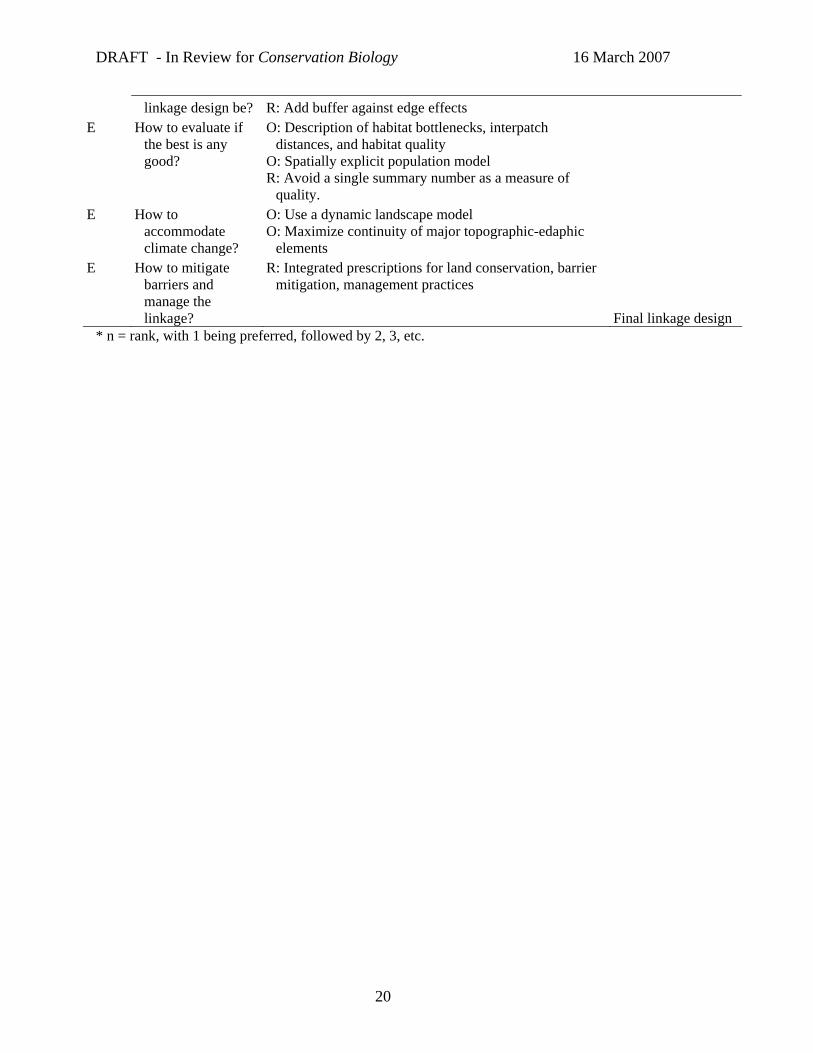
How to evaluate if the best is any good?

GIS least-cost procedures will always produce a least cost corridor or path – even if the best is entirely inadequate for the focal species. Therefore linkage designs should assess how well the linkage design serves each species, and how connectivity provided by the linkage after build-out compares to other benchmarks (such as connectivity under existing conditions, or an alternative linkage design). A conventional estimate of cost-weighted distance is a poor assessment metric because it does not indicate the level of interpatch movement or gene flow. At first glance, a spatially-explicit population model seems promising because it estimates the ability of a landscape configuration to maintain metapopulations of focal species (Carroll et al. 2003; Haines et al. 2006). However, uncertainty in such models precludes any meaningful estimate of risk of extinction and thus they provide only a ranking of alternatives (Beissinger & Westphal 1998). This underscores the need to derive resistance values from empirical estimates of interpatch movement or gene flow, such that differences will have a biological meaning. Promising tools such as graph theory (Theobald 2006) and isolation by resistance (McRae 2006) similarly depend on biologically-meaningful units of pixel resistance.

Until such resistance measures are developed, linkage designers must provide conservation investors and other stakeholders with meaningful descriptions of

how well the linkage design is expected to serve each focal species. For example, Larkin et al. (2004) reported the number of road crossings and the number and severity of bottlenecks in alternative corridors. Beier et al. (2007) provided frequency distributions of species-specific habitat quality in the linkage design and described the longest distances an individual animal would have to move between potential breeding patches. In cases where the interpatch distances exceeded the species’ estimated dispersal ability, South Coast Wildlands (2003-2006) and Beier et al. (2007) acknowledged that the linkage design probably would not provide meaningful connectivity for that species. South Coast Wildlands (2003-2006) and Beier et al. (2007) also used these descriptors to evaluate linkage utility for species (some birds, plants, and volant insects) for which habitat patches could be mapped but whose interpatch movement could not be modeled. Furthermore, they added patches of suitable habitat to the linkage design when such addition significantly reduced the length of interpatch dispersal movements required for one of these species.

A significant advance would be to create a GIS tool that would generate these statistics for any linkage design polygon of interest to stakeholders. For instance, this tool would enable a conservation investor to compare the biological optimum to a set of parcels meeting a cost constraint or other conservation goal. In some cases (e.g. evaluating invasion of exotic species via a linkage design) it may also be informative to compare the design to the option of not conserving a linkage (modeled by the conversion of all matrix land to human uses).

How to accommodate climate change?

All least-cost models include natural vegetation as a key driver; vegetation in turn is determined largely by climate, soils, and topography. Within the next 50 years, one of these factors, climate, will change enough to cause major shifts and reassembly of vegetation communities (Intergovernmental Panel on Climate Change 2001: Section 5.2.2.2). Williams et al. (2005) designed a linkage to allow endemic plants to shift their geographic range in response to climate change. Their procedure modeled suitable habitat at intervals of a decade, and identified spatially and temporally contiguous chains of 2.9-km2 grid cells with suitable habitat. Beier et al. (2006, 2007) assumed that a diversity of topographic elements (combinations of elevation, slope, and aspect such as high elevation flats,

10


north-facing slopes, or lowland flats) would support relatively continuous strands of whatever native vegetation communities will be present after climate change. They therefore evaluated their linkage designs for continuity of major topographic elements and expanded the linkage design to increase such continuity as needed. Their procedure would be improved by considering soil type in addition to topography, and by using an objective multivariate procedure to identify the major edaphic-topographic elements in a region. There is enormous room for other innovation on this important issue.

How to mitigate barriers and manage the linkage?

We advocate that linkage designs should comprehensively address land conservation, barrier mitigation, and land management practices. Unfortunately, most published linkage designs have one product, namely a map highlighting lands for conservation. There is a largely separate literature on wildlife-friendly highway crossing structures and other mitigations for highways and canals (e.g., National Highway Cooperative Research Program 2004; National Research Council 2005; Ventura County 2005; online proceedings of the International Conferences on Ecology and Transportation – www.icoet.net/). Conserving land will not create a functional linkage if major barriers are not mitigated, an excellent crossing structure will not create a functional linkage if the adjacent land is urbanized, and an integrated land acquisition-highway mitigation project could be jeopardized by inappropriate practices (e.g., predator control, fencing, artificial night lighting).

South Coast Wildlands (2003-2006) and Beier et al. (2007) used field observations to develop fine-scale recommendations for crossing structures, and management practices to restore native vegetation and minimize the impact of exotic species, fences, pets, livestock, and artificial night lighting. These management recommendations are especially important where people already live in or adjacent to the linkage design and must be engaged as its stewards. An emerging issue is how to mitigate the impact of fences, mowed strips, and stadium lighting designed to discourage human traffic on international borders.

Coda

Burgman et al. (2005) argue that choice of model frame (deciding what aspects of reality to model or ignore) is the most important type of uncertainty affecting

conservation planning, and that robust conservation plans must examine the choices, biases, and assumptions inherent in the model frame. We have called attention to several choices and assumptions that deserve serious attention. For instance, the idea that terrestrial animals choose movement paths based on the same rules they use to select habitat seems reasonable. However, Horskins et al. (2006) documented that a corridor with suitable habitat failed to promote gene flow, while Haddad & Tewksbury (2005) documented that low-quality habitat linkages promoted wildlife movement. Although these results do not falsify this assumption, they do suggest that it is not universally true, and that linkage designers must confront their assumptions and uncertainties.

Modeling uncertainty exists at each of the decision nodes described herein, and uncertainty may propagate from one node to the next. Although errors at successive points may offset each other, they may also be compounded to produce large uncertainty in the linkage design. Indeed as we bring all these issues to light, even avid designers like ourselves must question the value of our efforts. But despair is not an option in the face of unrelenting pressure to fragment landscapes. Instead we urge conservation biologists to continue to design wildlife linkages, be honest about uncertainties and assumptions, work to reduce uncertainty where possible, and describe the impact of uncertainty on the linkage design.

We have called for sensitivity analysis several times in this paper. The basic idea is to determine how much the corridor or linkage design changes when various options are chosen. We call attention to three issues in sensitivity analyses:

First, there are many possible interactions among choices. A small handful of options at each of the 16 choices described here will generate tens of thousands of combinations – more than anyone can feasibly subject to a sensitivity analysis (but see McCarthy et al. 1995). Therefore, most sensitivity analyses will consider only one choice, or at most three choices in combination. This sort of analysis cannot reveal how the results would differ under different background conditions (combinations of the choices not tested). However, even a constrained sensitivity analysis can suggest steps needed to reduce uncertainty and provide stakeholders with useful information. Any design robust to some assumptions is superior to a best guess lacking sensitivity analysis.

11

http://www.icoet.net/


Second, the sensitivity analysis will depend on the landscape under consideration, and cannot be extrapolated to other landscapes. In any particular landscape, stakeholders may only want to know if this linkage design is robust to its assumptions, in which case generalizability is not an issue. However, to advance the science of conservation planning, we recommend conducting sensitivity analyses on a diverse spectrum of artificial or real landscapes to identify the types of landscapes for which an approach is appropriate.

Third, the main question in sensitivity analysis is how a choice affects the location or effectiveness of the least-cost corridor for each focal species. Errors probably tend to compound through the processes reflected in the first 11 decision points described herein. As a result, each single-species corridor is probably less robust than conservation biologists would like. However, the processes reflected in the last five choices (those labeled E in Table 3) probably mitigate some error and uncertainty in the individual species models. In particular, adding focal species and widening the linkage to minimize edge effects or as a hedge against climate change will tend to decrease the risk that habitat important to any individual species is poorly covered by the linkage design.

At only a few decision points do we feel confident in knowing the “right choice.” For instance, we unhesitatingly recommend using multiple instead of single focal species, special procedures for corridor dwellers, and considering the impact of climate change. But for most junctures, we have merely put up a road sign warning of an approaching intersection and what sort of hazards might lie there. We believe that greatest progress will be made by building resistance models based on factors that are comprehensive, and developing an objective, biologically meaningful measure of resistance. We hope our roadmap will facilitate learning, provoke discussion and new approaches, improve the science of linkage design, and ultimately conserve biodiversity in a world increasingly dominated by human activity.

ACKNOWLEDGMENTS

The southern California linkage designs described by Beier et al. (2006) are available at www.scwildlands.org. An ArcGIS Toolbox with many of these GIS procedures, parameterized models for about 25 species (limited to vegetation types occurring in Arizona), and tools to compare alternative linkage

polygons, are available at www.corridordesign.org2. The designs produced by South Coast Wildlands were supported by The Wildlands Conservancy, Resources Legacy Fund Foundation, The California Resources Agency, US Forest Service, The Nature Conservancy, California State Parks, US National Park Service, Santa Monica Mountains Conservancy, Conservation Biology Institute, San Diego State University Field Stations, Southern California Wetlands Recovery Project, Mountain Lion Foundation, California State Parks Foundation, Environment Now, Anza Borrego Foundation, Summerlee Foundation, Zoological Society of San Diego, and South Coast Wildlands. The South Coast Wildlands approach was developed by PB, C. Cabañero, K. Daly, C. Luke, K. Penrod, E. Rubin, and WS. The Arizona Missing Linkages Project was supported by Arizona Game and Fish Department, Arizona Department of Transportation, U.S. Fish and Wildlife Service, U.S. Forest Service, Federal Highway Administration, Bureau of Land Management, Wildlands Project, and Northern Arizona University. Over the past 5 years, we discussed these ideas with A. Atkinson, T. Bayless, C. Cabañero, L. Chattin, M. Clark, K. Crooks, K. Daly, B. Dickson, R. Fisher, E. Garding, M. Glickfeld, N. Haddad, J. Jenness, S. Loe, T. Longcore, C. Luke, L. Lyren, B. McRae, S. Morrison, S. Newell, R. Noss, K. Penrod, E. J. Remson, S. Riley, E. Rubin, R. Sauvajot, D. Silver, J. Stallcup, and M. White. We especially thank the many government agents, conservationists, and funders who conserve linkages and deserve the best possible science.

LITERATURE CITED Adriaensen, F., J. P. Chardon, G. deBlust, E. Swinnen, S.

Villalba, H. Gulinck, and E. Matthysen. 2003. The application of ‘least-cost’ modeling as a functional landscape model. Landscape and Urban Planning 64:233-247.

Adriaensen, F., M. Githiru, J. Mwang’ombe, E. Matthysen, and L. Lens. 2007. Restoration and increase of connectivity among fragmented forest patches in the Taita Hills, Southeast Kenya. Part II Technical Report, CEPF project 1095347968. University of Gent, Gent, Belgium.

Andelman, S., I. Ball, F. Davis, and D. Stoms. 1999. SITES Version 1.0: an analytic toolbox for designing ecoregional conservation portfolios. The Nature Conservancy, Boise, Idaho.

2 The tools and models will be available at no cost. This site will be operational by the time this is published.

12

http://www.corridordesign.org/


Bani, L., M. Baietto, L. Bottoni, and R. Massa. 2002. The use of focal species in designing a habitat network for a lowland area of Lombardy, Italy. Conservation Biology 16:826-831.

Beier, P., K. Penrod, C. Luke, W. Spencer, and C. Cabañero. 2006. South Coast Missing Linkages: restoring connectivity to wildlands in the largest metropolitan area in the United States. Pages 555-586 in K. R. Crooks and M. A. Sanjayan, editors. Connectivity conservation. Cambridge University Press, Cambridge, U. K.

Beier, P., D. R. Majka, and T. Bayless. 2007. Eight linkage designs for Arizona’s missing linkages. Arizona Game and Fish Department, Phoenix. available from http://arizona.corridordesign.org/ (accessed March 2007)

Beier, P., and R. F. Noss. 1998. Do habitat corridors provide connectivity? Conservation Biology 12:1241-1252.

Beier, P., and S. Loe. 1992. A checklist for evaluating impacts to wildlife movement corridors. Wildlife Society Bulletin 20:434-440.

Beissinger, S. R. and M. I. Westphal. 1998. on the use of demographic models of population viability in endangered species management. Journal of Wildlife Management 62:821-841.

Berry, O, M. D. Tocher, D. M. Gleeson, and S. D. Sarre. 2005. Effect of vegetation matrix on animal dispersal: genetic evidence from a study of endangered skinks. Conservation Biology 19:855-864.

Brooks, T. M., da Fonseca, G. A. B., and A. S. L. Rodrigues. 2004. Species, data, and conservation planning. Conservation Biology 18:1682-1688.

Broquet, T., N. Ray, E. Petit, J. M. Fryxell, and F. Burel. 2006. Genetic isolation by distance and landscape connectivity in the American marten Martes americana. Landscape Ecology. 21:877-889

Bunn, A.G., D.L. Urban, and T.H. Keitt. 2000. Landscape connectivity: A conservation application of graph theory. Journal of Environmental Management 59:265-278.

Burgman, M. A., D. B. Lindenmayer, and J. Elith. 2005. Managing landscapes for conservation under uncertainty. Ecology 86:2007-2017.

Carr, M. H., T. D. Hoctor, C. Goodison, P. D. Zwick, J. Green, P. Hernandez, C. McCain, J. Teisinger, K. Whitney. 2002. Final Report. Southeastern Ecological Framework. The GeoPlan Center, University of Florida, Gainesville, Florida.

Carroll, C., R. F. Noss, P. C. Paquet, and N. H. Schumaker. 2003. Use of population viability analysis and reserve selection algorithms in regional conservation plans. Ecological Applications 13:1773-1789.

Clevenger, A. P., J. Wierzchowski, B. Chruszcz, and K. Gunson. 2002. GIS-directed, expert-based models for identifying wildlife habitat linkages and planning mitigation passages. Conservation Biology 16:503-514.

Dickson, B. G., and P. Beier. 2007. Quantifying the influence of topographic position on cougar movement in southern California USA. Journal of Zoology

(London) 271:270-277. Dixon, J. D., M. K. Oli, M. C. Wooten, T. H. Eason, J. W.

McCown, and D. Paetkau. 2006. Effectiveness of a regional corridor in connecting two Florida black bear populations. Conservation Biology 20:155-162.

Epps, C. W., P. Palsboell, J. D. Wehausen, G. K. Roderick, R. Ramey, and D. R. McCullough. 2005. Highways block gene flow and cause a rapid decline in genetic diversity of desert bighorn sheep. Ecology Letters 8:1029-1038.

Environmental Law Institute. 2003. Conservation thresholds for land use planners. Environmental Law Institute, Washington D.C. Available from www.elistore.org (accessed March 2007).

Fahrig, L., and G. Merriam. 1994. Conservation of fragmented populations. Conservation Biology 8:50-59.

Ferreras, P. 2001. Landscape structure and asymmetrical inter-patch connectivity in a metapopulation of the endangered Iberian lynx. Biological Conservation 100:125-136.

Fleury, A. M., and R. D. Brown. 1997. A framework for the design of wildlife conservation corridors with specific application to southwestern Ontario. Landscape and Urban Planning 37:163-186.

Gerlach, G., and K. Musolf. 2000. Fragmentation of landscape as a cause for genetic subdivision in bank voles. Conservation Biology 14:1066-1074.

Glenn, E. M., and W. J. Ripple. 2004. On using digital maps to assess wildlife habitat. Wildlife Society Bulletin 32:852-860.

Graham, C. 2001. Factors influencing movement patterns of keel-billed toucans in a fragmented tropical landscape i southern Mexico. Conservation Biology 15:1789-1798.

Guisan, A., and W. Thuiller. 2005. Predicting species distribution: offering more than simple habitat models. Ecology Letters 8:993-1009.

Haddad, N. M., D. R. Bowne, A. Cunningham, B. J. Danielson, D. J. Levey, S. Sargent, and T. Spira. 2003. Corridor use by diverse taxa. Ecology 84:609-615.

Haddad, N. M., and J. J. Tewksbury. 2005. Low-quality habitat corridors as movement conduits for two butterfly species. Ecological Applications 15:250-257.

Haines, A. M., M. E. Tewes, and J. Young. 2006. Habitat based population viability analysis of ocelots in southern Texas. Biological Conservation 132:424-436.

Hargrove, W. W., F. M. Hoffman, and R. A. Efroymson. 2004. A practical map-analysis tool for detecting potential dispersal corridors. Landscape Ecology 20:361-373.

Harrison, R. L. 1992. Toward a theory of inter-refuge corridor design. Conservation Biology 6:293-295.

Hoctor, T. S., M. H. Carr, and P. D. Zwick. 2000. Identifying a linked reserve system using a regional landscape appraoach: the Florida Ecological Network. Conservation Biology 14:984-1000.

Horskins, K., P. B. Mather, and J. C. Wilson. 2006. Corridors and connectivity: when use and function do not

13

http://arizona.corridordesign.org/

http://www.elistore.org/


equate. Landscape Ecology 21:641-655. Hunter, R. D., R. N. Fisher, and K. R. Crooks. 2003.

Landscape-level connectivity in coastal southern California USA as assessed through carnivore habitat suitability. Natural Areas Journal 23:302-314.

Intergovernmental Panel on Climate Change. 2001. Climate Change 2001: Synthesis. Third Assessment Report. United Nations Environment Program, Geneva.

Joly, P., S. Morand, and A. Cohas. 2003. Habitat fragmentation and amphibian conservation: building a tool for assessing landscape matrix connectivity. C. R. Biologies 326:S132-S139.

Jordán, F. 2000. A reliability-theory approach to corridor design. Ecological Modelling 128:211-220.

Jordán, F., A. Baldi, M-M. Orci, I. Racz, and Z. Varga. 2003. Characterizing the importance of habitat patches and corridors in maintaining the landscape connectivity of a Pholidoptera tanssylvanica (Orthoptera) metapopulation. Landscape Ecology 18:83-92.

Kautz, R., R. Kawula, T. Hoctor, J. Comiskey, D. Jansen, D. Jennings, J. Kasbohm, F. Mazzotti, R. McBride, L. Richardson, and K. Root. 2006. How much is enough? landscape level conservation for the Flroida panther. Biological Conservation 130:118-133.

Kobler, A., and M. Adamic. 1999. Brown bears in Slovenia: identifying locations for construction of wildlife bridges across highways. In: Evink, G.; Garrett, P. Zeigler, D. eds. Proceedings of International Conference on Ecology and Transportation. not paginated, available at http://www.icoet.net/ICOWET/99proceedings.asp.

Larkin, J. L., D. S. Maehr, T. S. Hoctor, M. A. Orlando, and K. Whitney. 2004. Landscape linkages and conservation planning for the black bear in west-central Florida. Animal Conservation 7:23-34.

Malczewski, J. 2000. On the use of weighted linear combination method in GIS: common and best practice approaches. Transactions in GIS 4:5-22.

Marulli, J., and J. M. Mallarach. 2005. A GIS methodology for assessing ecological connectivity: application to the Barcelona Metropolitan Area. Landscape and Urban Planning 71:243-262.

McRae, B. 2006. Isolation by resistance: a model of gene flow in heterogeneous landscapes. Evolution 60:1551-1561.

McCarthy, M. A., M. A. Burgman, and S. Ferson. 1995. Sensitivity analysis for models of population viability. Biological Conservation 73:93-100.

Millspaugh, J. J., and J. M. Marzluff. 2001. Radio tracking and animal populations. Academic Press, San Diego, California..

National Highway Cooperative Research Program. 2004. Environmental stewardship practices, procedures, and policies for highway construction and maintenance. Transportation Research Board, Washington D.C.

National Research Council. 2005. Assessing and managing

the ecological impacts of paved roads. NRC Press, Washington D.C.

Newell, S. L. 2006. An evaluation of a science-based approach to habitat linkage design. M.S. Thesis, Northern Arizona University, Flagstaff, Arizona.

Noss, R. F., and K. M. Daly. 2006. Incorporating connectivity into broad-scale conservation planning. Pages 587-619 in K. R. Crooks and M. A. Sanjayan, editors. Connectivity conservation, Cambridge University Press, Cambridge, U.K.

Possingham, H. P., I. R. Ball, and S. Andelman. 2000. Mathematical methods for identifying reserve networks. Pages 291-306 in S. Ferson and M. Burgman, editors. Quantitative methods for conservation biology. Springer-Verlag, New York.

Quinby, P., S. Trombulak, T. Lee, J. Lane, M. Henry, R. Long, and P. MacKay. 1999. Opportunities for wildlife habitat connectivity between Algonquin Provincial Park and the Adirondack Park. Ancient Forest Exploration and Research, Powassan, Ontario.

Rouget, M., R. M. Cowling, A. T. Lombard, A. T. Knight, and G. H. Kerley. 2006. Designing large-scale conservation corridors for pattern and process. Conservation Biology 20:549-561.

Schadt, S., F. Knauer, P. Kaczensky, E. Ravilla, T. Wiegand, and L. Trep. 2002. Rule-based assessment of suitable habitat and patch connectivity for the Eurasian lynx. Ecological Applications 12:1469-1483.

Servheen, C., J. S. Walker, and P. Sandstrom. 2001. Identification and management of linkage zones for grizzly bears between the large blocks of public land in the northern Rocky Mountains. Proceedings of International Conference on Ecology and Transportation 161-179.

Singleton, P. H., W. L. Gaines, and J. F. Lehmkuhl. 2002. Landscape permeability for large carnivores in Washington: a geographic information system weighted-distance and least-cost corridor assessment. Research Paper PNW-RP-549. 89.

South Coast Wildlands (lead authors: K. Penrod, C. Cabañero, P. Beier, C. Luke. W. Spencer, and E. Rubin. S. Loe, K. Keyer, R. Sauvajot, S. Shapiro, and D. Kamradt co-authored some reports). 2003-2006. Linkage designs for the South Coast ecoregion of California. available from scwildlands.org (accessed March 2007).

Southern Rockies Ecosystem Project. 2005. Linking Colorado’s landscapes: a statewide assessment of wildlife linkages, Phase I report. Southern Rockies Ecosystem Project, Denver, Colorado.

Sutcliffe, O. L., V. Bakkestuen, G. Fry, and O. D. Stabbetorp. 2003. Modelling the benefits of farmland restoration: methodology and application to butterfly movement. Landscape and Urban Planning 63:15-31.

Theobald, D. M. 2006. Exploring the functional connectivity of landscapes using landscape networks. Pages 416–443 in K. R. Crooks and M. A. Sanjayan, editors,

14


Connectivity conservation, Cambridge University Press, Cambridge. U. K.

Urban, D., and T. Keitt. 2001. Landscape connectivity: a graph-theoretic perspective. Ecology 82:1205-1218.

US Fish and Wildlife Service. 1981. Standards for the development of Suitability Index Models. Division of Ecological Services, Government Printing Office, Washington DC.

van Langevelde, F. 2000. Scale of habitat connectivity and colonization in fragmented nuthatch populations. Ecography 23:614-622.

Ventura County. 2005. Guidelines for safe wildlife passage. Ventura County Planning Devision, Ventura, CA USA. 45pp.

Verbeylen, G., L. De Bruyn, .F Adriaensen, and E. Matthysen. 2003. Does matrix resistance influence red squirrel (Sciurus vulgaris L. 1758) distribution in an urban landscape? Landscape Ecology 18:791-805.

Walker, R. and L. Craighead. 1997. Analyzing wildlife movement corridors in Montana using GIS. 1997. Environmental Sciences Research Institute. Proceedings of the 1997 International ESRI Users conference. not paginated, available from http://gis.esri.com/library/userconf/proc97/proc97/to150/pap116/p116.htm (accessed March 2007).

Wikramanayake, E., M. McKnight, E. Dinerstein, A. Joshi, B. Gurung, and D. Smith. 2004. Designing a conservation landscape for tigers in human-dominated ecosystems. Conservation Biology 18:839-844.

Wilcove, D. S., C. H. McLellan, and A. P. Dobson. 1986. Habitat fragmentation in the temperate zone. Pages 237-256 in M. E. Soulé, editor, Conservation biology: the science of scarcity and diverstiy. Sinauer, Sunderland, Massachusetts.

Wilcox, B. A., and D. D. Murphy. 1985. Conservation strategy: the effects of fragmentation on extinction. American Naturalist 125:879-887.

Williams, P., L. Hannah, S. Andelman, G. Midgley, M. Araujo, G. Hughes, L. Manne, E. Martinez-Meyer, and R. Pearson. 2005. Planning for climate change: identifying minimum-dispersal corridors for the cape Protaceae. Conservation Biology 19:1063-1074.

Yang, L., S. V. Stehman, J. H. Smith, and J. D. Wickham. 2001. Thematic accuracy of MRLC land cover for the eastern United States. Remote Sensing of Environment 76:418-422.

15


Table 1. Studies that produced maps of corridors, linkages, or cost surfaces to guide conservation decisions in the mapped landscape. Author & Year of Publication(s)

Focal species or Focal ecological condition

Habitat Factorsa

Map productb

How resistance values were estimated

Decisions subject to sensitivity analysis

Adriaensen et al. 2007

8 birds, forest butterflies

L R E Corridor Expert opinion, research on target species in linkage area

Resistance values

Bani et al. 2002 9 birds, 3 carnivores

L Path Empirical data on relative abundance of focal species in linkage area

None

South Coast Wildlands (2003-2006), Beier et al. 2006; Newell 2006

10 or more mammals, reptiles, amphibians, fish, birds, invertebrates, or plans per linkage

L R E T Corridor Expert opinion and literature review

Resistance values, factor weights, number of focal species

Beier et al. 2007 10 or more mammals, reptiles, & amphibians per linkage

L R E T Corridor Expert opinion and literature review

None

Carr et al. 2002 Naturalness L R Cost map

Expert opinion and literature review

Graham 2001 Ramphastos sulfuratus

L Path Empirical data on habitat use and movement in linkage area

Resistance values

Hoctor et al. 2000 Naturalness L R Edge Corridor Expert opinion and literature review

None

Hunter et al. 2003 Lynx rufus, Puma concolor

L R Cost map


None

Joly et al. 2003 Bufo bufo L R Cost map


None

Kautz et al. 2006 Puma concolor L Path Empirical data on habitat use in linkage areas

Resistance values

Kobler and Adamic 1999

Ursus arctos L Path empirical data on animal occurrences in linkage area

None

Larkin et al. 2004 Ursus arctos L R Path Expert opinion and literature review

Resistance values

Marulli and Mallarach 2005

Naturalness L R Corridor Expert opinion and literature review

None

Quinby et al. 1999

Canis lupus L R N W Corridor Expert opinion and literature review

Resistance values, factor weights

Schadt et al. 2002 Lynx canadensis L R Path Empirical data on habitat use in linkage areas

Resistance values

Servheen et al. 2001

Ursus arctos L R Cost map


None

16


Singleton et al. 2002

Canis lupus, Gulo gulo, Lynx canadensis, Ursus arctos, “general carnivore”

L R N E S Corridor lit review and expert opinion None

Sutcliffe et al. 2003

2 butterfly species L Path Empirical data on interpatch movement (best fit of 5 vectors)

Nonec

Walker & Craighead 1997

Ursus arctos, Puma concolor, Cervus elaphus

L R Edge Cost map


None

Wikramanayake et al. 2004

Panthera tigris L E Cost map

Expert opinion None

Williams et al. 2005

The plant family Protaceae

L C Path Not applicabled None

a L = Land cover and land use, R = road density or proximity to roads, or road presence mapped as a land cover type, N = human population size. E = Elevation, Edge = Edge between land cover/land use types, T = Topographic feature, S = slope, W = proximity to water, C = Climate envelope model. b Path = pixel-wide patch (pixels were 2.9-km2 cells for Williams et al. 2005). Corridor = slice encompassing the most permeable percentiles of the cost map. Cost map = cumulative resistance displayed as a gradient, without explicitly stating a threshold percentile constituting the recommended corridor. c Some sensitivity analysis to resistance values occurred in fitting resistance values to interpatch movement data. d Resistance was not explicitly calculated. Each species was assumed to disperse to all cells with predicted suitable climate within its dispersal distance.

17


Table 2. When assumptions and choices are not clearly explained, focal-species approaches to linkage design may provoke objections. Linkage designers can address most issues by appropriate choices during the GIS modeling process. Objection Relevant Choices (Table 3) A linkage designed to conserve focal species may fail to

conserve ecological processes. Which focal species? How wide should the linkage

design be? How to accommodate climate

change?

A corridor designed for 1 or 2 large carnivores (often highly mobile habitat generalists) probably will not serve other species.

Which focal species?

The model uncritically assumes that animals use the same rules to make movement decisions as they use to select habitat.

How to estimate resistance for each class of pixels?


Animals choose habitat and make movement decisions based on availability of food and mates, and safety from predators and hazards, but the model is based on a few factors widely available in GIS format.

What landscape factors to include in the model?

Because climate change will change the land cover map used in the model, the linkage design will fail.

How to accommodate climate change?

The least-cost model always produces a “best” route, but the best may not be good enough to allow movement & gene flow.


GIS models based on movement are not appropriate for species that need several generations to move their genes through a linkage.


A linkage may facilitate movement of invasive species. Which focal species? How wide should the linkage

design be? How to mitigate barriers and

manage the linkage?

The expense of implementing the linkage design outweighs its benefits.


Least-cost modeling ignores some plants, insects, and birds whose movement can’t be modeled in this framework.


18


Table 3. Decisions in GIS approaches to linkage design, corresponding to a logical sequence of analytic steps, options and recommended actions at each decision point, and GIS outputs at various stages of the analysis.

Box (Table 1)

Decision Recommendation (R), Options (O), and Ranked Options (On)*

Product at this point of the analysis

A How to define the analysis area?

R: Rectangle including facing edges of wildland blocks, intervening matrix, and facilitating elements

B Which focal species? R: Multiple species, chosen to represent ecological processes, sensitivity to barriers, etc.

B Which landscape factors to include in the model?

R: Try to use a comprehensive set of factors. R: Acknowledge when available data layers are not

comprehensive. B What metric for each

factor? R: Report source, resolution and accuracy of data

B How to estimate resistance for each class of pixels?

O1: Genetic distance O2: Interpatch movements O3: Resource selection function O4: Literature review & expert opinion

Resistance value for each class within each factor

B How to combine factors?

O: Weighted sum O: Weighted product O: Geometric mean R: display maps showing sensitivity of predicted linkage

to this choice and previous choice B How to delineate a

corridor terminus? R: For analysis purposes, “pull back” the facing edges of

nearly-touching blocks to give the model “room to run.” R: Each terminus should correspond to potential or

known population B Whether and how to

delineate habitat patches?

R: Do map potential breeding patches to help define terminuses, increase the likelihood that the modeled corridor will encompass steppingstones, and as a tool to evaluate utility of the linkage design.

B How to model corridor dwellers?

R: Assign minimum resistance to breeding patches that are within effective dispersal distance of patches already included.

Resistance for each pixel

C How to identify continuous swaths of low-resistance pixels?

O: Lowest cumulative resistance O: Individual-based movement model

Cost map of matrix D How wide should a

single-species corridor be?

R: For corridor dwellers, width should be substantially more than a home range width.

R: Iterative mapping to identify acceptable number and severity of bottlenecks

Least-cost corridor for one focal species

E How to combine corridors of multiple focal species?

R: Union that covers all focal species, but trim redundant strands to minimize area and edge

Preliminary linkage design

E How wide should the R: “No regret” standard

19


20

linkage design be? R: Add buffer against edge effects E How to evaluate if

the best is any good?

O: Description of habitat bottlenecks, interpatch distances, and habitat quality

O: Spatially explicit population model R: Avoid a single summary number as a measure of

quality.

E How to accommodate climate change?

O: Use a dynamic landscape model O: Maximize continuity of major topographic-edaphic

elements

E How to mitigate barriers and manage the linkage?

R: Integrated prescriptions for land conservation, barrier mitigation, management practices

Final linkage design * n = rank, with 1 being preferred, followed by 2, 3, etc.


21

A. Define landscape to beanalyzed.

B. Develop algorithm toestimate resistance of a pixel as

a function of pixel attributes.

C. Produce a travel costmap for landscape.

D. Select swath of pixels withlowest cumulative travel cost.

E. Modify corridor design toaccommodate additional species orprocesses, or to reduce edge effects.

Figure 1. General flowchart for a GIS-based linkage design. The processes labeled A through E involve choices listed in Table 3 and described in the text.

Figure 2. Example of single-species corridors joined into a preliminary linkage design. The needs of different focal species produce multiple strands. Facilitating landscape elements (such as riparian areas) can produce deeply-looped strands.


22

A.

B. Figure 3. Modeling a corridor for a hypothetical focal species. (A) resistance of individual pixels. Note that low-resistance pixels need not form a continuous swath. (B) travel cost (cumulative resistance). Low-cost pixels always form continuous swaths and increasingly higher maximum costs define a nested set of increasingly broad “slices” of the landscape. As the cost threshold increases from slice 1 to slice 3 to achieve minimum width, w, the modeled corridor becomes very wide in areas outside the bottleneck. As the cost threshold increases even more (slice 4) the modeled corridor gains additional strands.

Date post:	17-Jun-2018
Category:	Documents
Upload:	nguyenthu
View:	213 times
Download:	0 times

DRAFT - In Review for Conservation Biology 16 March...

Documents