Draft Summary Page | 1 Draft Summary Report: Groundwater Modelling Dr. Catherine Moore, GNS Science Ltd. Dr. Mark Gyopari, Earth in Mind Ltd. 1. Groundwater Model Design Groundwater modelling is being undertaken using the USGS MODFLOW-MT3D programme suite. This has replaced the previous FEFLOW models (used for the conjunctive allocation modelling work) because MODFLOW can more easily and effectively allow integration with other models and will significantly enhance and speed up the calibration process. MODFLOW also has a more sophisticated surface water module (the SFR package – ‘Stream Flow Routing’) which will be coupled to the surface water contaminant model (eSource). SFR also receives inputs from Topnet and Irricalc– the former provides input steamflows into the model boundaries, whilst the latter provides irrigation takes from surface water and groundwater, and water inputs via groundwater recharge and near-surface lateral flow to streams. MODFLOW is run in conjunction with MT3D – which is a contaminant transport model which can simulate the advection, dispersion and transformation of contaminants in groundwater. Two connected MODLFOW models have been constructed. The Northern Model combines the previous Feflow Upper and Middle Valley models, and the Southern Model is equivalent to the previous Lower Valley Model. The geological and layer structure of the models has been transferred directly from the Felfow models in recognition that they embody extensive expert effort and represent our best understanding of the hydrogeological environments to date. The transient flow models currently run at 7-day time steps for the period 1992 – 2015 (although initial calibration runs are to 2007 to reduce turn-around-time). Fig A: New MODFLOW simulations for the Ruamahanga Valley – two models have been construction: the Northern and Southern models.
Transcript
Draft Summary Page | 1
Draft Summary Report: Groundwater Modelling Dr. Catherine Moore, GNS Science Ltd. Dr. Mark Gyopari, Earth in Mind Ltd.
1. Groundwater Model Design Groundwater modelling is being undertaken using the USGS MODFLOW-MT3D programme suite. This has replaced the previous FEFLOW models (used for the conjunctive allocation modelling work) because MODFLOW can more easily and effectively allow integration with other models and will significantly enhance and speed up the calibration process. MODFLOW also has a more sophisticated surface water module (the SFR package – ‘Stream Flow Routing’) which will be coupled to the surface water contaminant model (eSource). SFR also receives inputs from Topnet and Irricalc– the former provides input steamflows into the model boundaries, whilst the latter provides irrigation takes from surface water and groundwater, and water inputs via groundwater recharge and near-surface lateral flow to streams. MODFLOW is run in conjunction with MT3D – which is a contaminant transport model which can simulate the advection, dispersion and transformation of contaminants in groundwater.
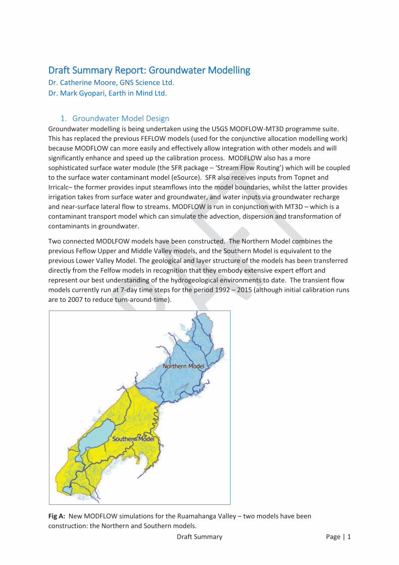
Two connected MODLFOW models have been constructed. The Northern Model combines the previous Feflow Upper and Middle Valley models, and the Southern Model is equivalent to the previous Lower Valley Model. The geological and layer structure of the models has been transferred directly from the Felfow models in recognition that they embody extensive expert effort and represent our best understanding of the hydrogeological environments to date. The transient flow models currently run at 7-day time steps for the period 1992 – 2015 (although initial calibration runs are to 2007 to reduce turn-around-time).
Fig A: New MODFLOW simulations for the Ruamahanga Valley – two models have been construction: the Northern and Southern models.
Draft Summary Page | 2
2. Groundwater model dependencies Fig B shows how other models in the modelling system support and connect to MODFLOW and MT3D. Principal inputs are provided by the soil moisture balance modelling performed by Irricalc which provides rainfall recharge, irrigation take and return water and runoff to the groundwater model. Irrigation water demand is assigned to relevant water take consents (groundwater or surface water). Topnet provides surface water flows from surrounding catchments into the model domains encompassing the plains. These supporting models are underpinned by a NIWA climate model, which provides simulated rainfall and potential evapotranspiration on a 500m2 grid, and LCR soil property data.
Overseer provides nitrate loadings for MT3D which calculates migration to groundwater and eventually discharge to surface water (to SFR boundaries). Exchange of flow (between groundwater and surface water in either direction), and nitrate loading data between SFR and eSource occurs – in effect, these models are loosely coupled.
Fig B: Groundwater model dependencies.
3. Simulation of surface water – groundwater interaction The MODFLOW SFR (streamflow routing) module represent a key component of the overall modelling system which simulates flow and contaminant interactions between groundwater and the surface water environment. All major and minor water courses are represented by SFR segments (Fig C shows the Northern Model SFR segments). Channel geometries and depth-flow and flow-channel-width relationships used in the SFR boundaries have been derived using MIKE 11 models developed for the previous feflow modelling work. SFR is loosely coupled with the eSource model to assist in the simulation of surface water quality by contributing contaminant inputs from groundwater. SFR also allows water to be diverted for surface water abstractions (calculated by Irricalc) and water race diversions.
Draft Summary Page | 3
Fig C: Surface water bodies included in the Northern Model
Calibration of the Groundwater – Surface water modelling in the Ruamahanga Background The groundwater and surface flow in the Ruamahanga is being simulated using a MODFLOW model which incorporates a stream flow routing package. The transport of the contaminants in groundwater and into surface waterways is being simulated using the MT3D software which connects to MODFLOW.
The parameters in this flow and transport model are being estimated using the parameter estimation software ‘PEST’. The reliability of parameter estimates (or uncertainty analysis) is also being quantified using a linear Bayesian analysis incorporated in PEST. The model parameters being adjusted in this calibration process are:
Groundwater hydraulic parameters (hydraulic conductivity, storativity and porosity) Stream bed conductance
The hydraulic parameters are located at the pilot-point locations shown in Figure 1 in all model layers. The pilot point values are spatially interpolated to provide parameter inputs for the entire model grid. The stream bed conductance parameters are estimated for each separate stream segment. Note the sparser spread of pilot points in the southern model was required due to the much longer model run times of the southern model.
Draft Summary Page | 4
Figure 1. Location of pilot points where the groundwater hydraulic parameters are estimated
Data and assumptions The data the model uses can be separated into ‘input data’ and ‘calibration target data’. The input data is described variously in the groundwater model development report (Mark Gyopari), the estimate of nitrate input fluxes in the Jacobs report (Michelle Greenwood), and the estimate of rainfall recharge and runoff and water abstraction volumes are included in the Irricalc report (John Bright).
The data the model is calibrated to (e.g. calibration target data) includes:
measured groundwater levels, surface water flows, surface water simultaneous gaugings (so that losses and gains to groundwater from surface
water are identified) and concentrations in groundwater.
Draft Summary Page | 5
Groundwater levels The location of groundwater level monitoring sites and their long term average water levels is shown in Figure 3. Long term water levels from 1992 to 2007 have been recorded at these sites. The spatial density of monitoring sites is greater in the northern groundwater model.
Figure 2 Location of long term groundwater level monitoring sites
Draft Summary Page | 6
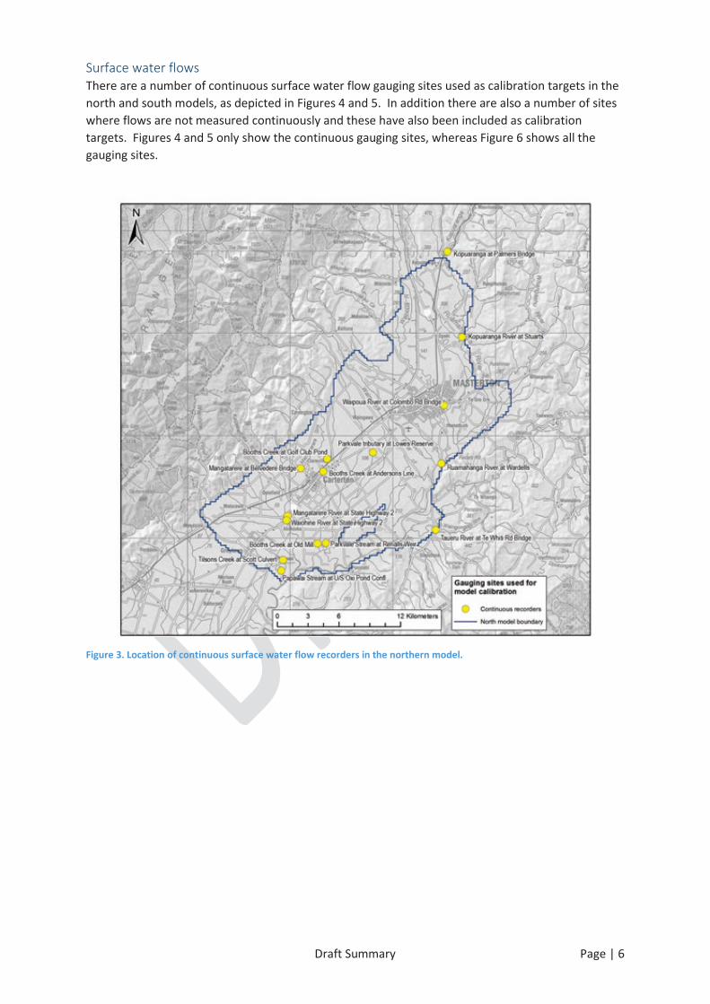
Surface water flows There are a number of continuous surface water flow gauging sites used as calibration targets in the north and south models, as depicted in Figures 4 and 5. In addition there are also a number of sites where flows are not measured continuously and these have also been included as calibration targets. Figures 4 and 5 only show the continuous gauging sites, whereas Figure 6 shows all the gauging sites.
Figure 3. Location of continuous surface water flow recorders in the northern model.
Draft Summary Page | 7
Figure 4. Location of continuous surface water flow recorders in the Southern model.
Draft Summary Page | 8
Figure 5. Location of all surface water flow sites used in the model calibration
Nitrate concentration data The nitrate concentration trends in groundwater have been monitored at the sites depicted in Figure 7. These sites have been combined with shorter term and one off concentration measurements to provide a plot of average nitrate concentrations in the modelled area, shown in Figure 8, which indicate some ‘hot spot’ areas of higher nitrate concentrations do occur, particularly in the northern model. However only the sites shown in Figure 6 were selected as model calibration targets, as the nitrate inputs to the model from overseer represent ‘average’ nitrate losses, and hence sufficiently long nitrate concentration times series in groundwater were required to calculate a commensurate ‘average’ groundwater nitrate concentration. The locations shown in Figure 6 all had more than 10 measurements of nitrate concentrations.
In addition the nitrate concentrations in surface water also were analysed, as these surface water concentrations provide nitrate flux inputs to the MT3D model, in addition to the nitrate flux inputs from land surface recharge. These nitrate concentrations shown in Figure 9 are very sparse, are generally much lower than the groundwater concentrations, and vary considerably across the model and with time. Because of this lack of data, a fixed surface water concentration input that represents the average surface water nitrate concentrations across all sites was adopted in the model.
Draft Summary Page | 9
Figure 6. Location of long term groundwater nitrate concentration records
Draft Summary Page | 10
Figure 7. Average nitrate concentrations measured in groundwater in the modelled area.
Draft Summary Page | 11
Figure 8. Average nitrate concentrations in surface water
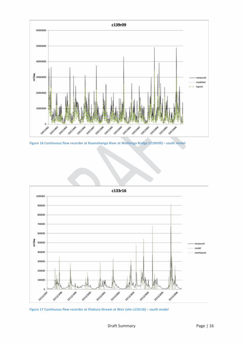
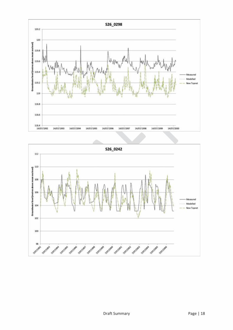
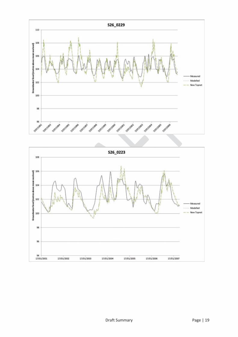
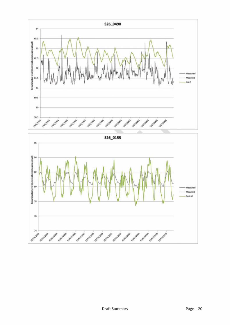
OOutputs In this section snapshots of the model to measurement matches are shown. As expected the model simulates some parts of the system very well, and less well in others. This range of model to measurement fits is experienced in all groundwater models, and occurs because the variations in strata below the ground can never be perfectly known on the basis of wells. To address this always incomplete knowledge, we describe the confidence limits around model outputs and the model parameters used in the model. Therefore all model simulated flows and groundwater levels have uncertainty associated with them, which is quantified in terms of confidence limits. So while we cannot say at all locations precisely what the model output is, we are always able to define the bounds that the model output will lie within. The impact that these uncertainties may have on scenario simulations are quantified for each scenario considered. This error is quantified using a Bayesian linear uncertainty analysis.
Draft Summary Page | 12
MMeasured and Modelled Surface water flows on the Plains
As mentioned above the model calibration process is continuing, however the model to measurement fits at selected surface water flow recorder sites and groundwater level recorder sites can be seen. The locations of these sites can be found in Figures 4 and 5.
Figures 10-18 depict the modelled and measured surface flows comparisons.
Figure 9. Continuous flow recorder at Ruamahanga River at Wardells (site c029r06)
Draft Summary Page | 13
Figure 10 Continuous flow recorder at Taueru River at Te Whiti Rd Bridge (site c042r11)
Figure 11 Continuous flow recorder at Parkvale Stream at Renalls Weir (site c065r07)
Draft Summary Page | 14
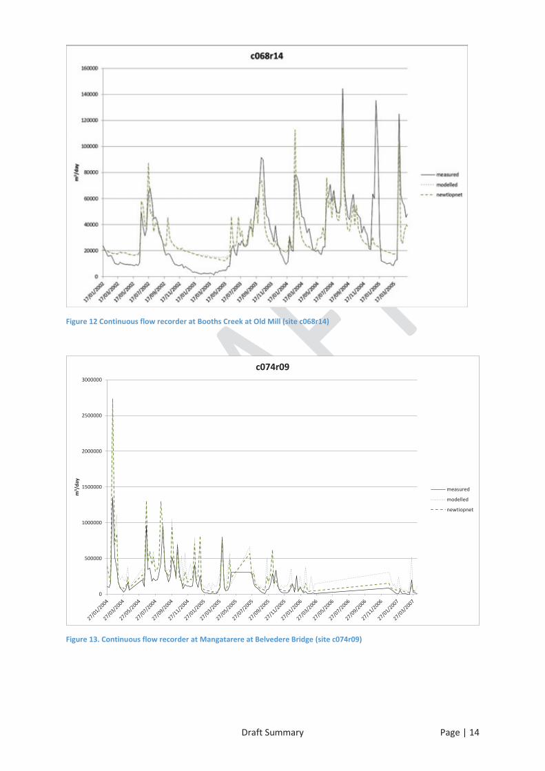
Figure 12 Continuous flow recorder at Booths Creek at Old Mill (site c068r14)
Figure 13. Continuous flow recorder at Mangatarere at Belvedere Bridge (site c074r09)
0
500000
1000000
1500000
2000000
2500000
3000000
m3 /
day
c074r09
measured
modelled
newtiopnet
Draft Summary Page | 15
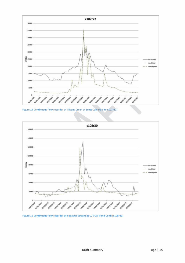
Figure 14 Continuous flow recorder at Tilsons Creek at Scott Culvert (site c107r22)
Figure 15 Continuous flow recorder at Papawai Stream at U/S Oxi Pond Confl (c108r30)
Draft Summary Page | 16
Figure 16 Continuous flow recorder at Ruamahanga River at Waihenga Bridge (c139r09) – south model
Figure 17 Continuous flow recorder at Otakura Stream at Weir (site c133r16) – south model