Draft version November 3, 2021 Typeset using L A T E X preprint2 style in AASTeX63 The Influence of 10 Unique Chemical Elements in Shaping the Distribution of Kepler Planets Robert F. Wilson, 1, 2 Caleb I. Ca˜ nas, 3, 4, * Steven R. Majewski, 1 Katia Cunha, 5, 6 Verne V. Smith, 7 Chad F. Bender, 6 Suvrath Mahadevan, 3, 4 Scott W. Fleming, 8 Johanna Teske, 9 Luan Ghezzi, 10 Henrik J¨ onsson, 11 Rachael L. Beaton, 12, 13, † Sten Hasselquist, 14, ‡ Keivan Stassun, 15 Christian Nitschelm, 16 D. A. Garc´ ıa-Hern´ andez, 17, 18 Christian R. Hayes, 19 and Jamie Tayar 20, 21, § 1 Department of Astronomy, University of Virginia, Charlottesville, VA 22904-4325, USA 2 NASA Goddard Space Flight Center, 8800 Greenbelt Road, Greenbelt, MD 20771, USA 3 Department of Astronomy & Astrophysics, The Pennsylvania State University, 525 Davey Laboratory, University Park, PA 16802, USA 4 Center for Exoplanets and Habitable Worlds, The Pennsylvania State University, 525 Davey Laboratory, University Park, PA 16802, USA 5 Observat´orio Nacional, Rua General Jos´ e Cristino, 77, Rio de Janeiro, RJ 20921-400, Brazil 6 Steward Observatory, University of Arizona, 933 North Cherry Avenue, Tucson, AZ 85721-0065, USA 7 NSF’s NOIRLab, 950 North Cherry Avenue, Tucson, AZ 85719, USA 8 Space Telescope Science Institute, 3700 San Martin Dr., Baltimore, MD 21218, USA 9 Carnegie Earth and Planets Laboratory, 5241 Broad Branch Road, NW, Washington, DC 20015 10 Universidade Federal do Rio de Janeiro, Observat´orio do Valongo, Ladeira do Pedro Antˆonio, 43, Rio de Janeiro, RJ 20080-090, Brazil 11 Materials Science and Applied Mathematics, Malm¨o University, SE-205 06 Malm¨o, Sweden 12 Department of Astrophysical Sciences, Princeton University, 4 Ivy Lane, Princeton, NJ 08544 13 The Observatories of the Carnegie Institution for Science, 813 Santa Barbara St., Pasadena, CA 91101 14 Department of Physics & Astronomy, University of Utah, Salt Lake City, UT, 84112, USA 15 Department of Physics and Astronomy, Vanderbilt University, VU Station 1807, Nashville, TN 37235, USA 16 Centro de Astronom´ ıa (CITEVA), Universidad de Antofagasta, Avenida Angamos 601, Antofagasta 1270300, Chile 17 Instituto de Astrof´ ısica de Canarias (IAC), E-38205 La Laguna, Tenerife, Spain 18 Universidad de La Laguna (ULL), Departamento de Astrof´ ısica, E-38206 La Laguna, Tenerife, Spain 19 Department of Astronomy, Box 351580, University of Washington, Seattle, WA 98195 20 Institute for Astronomy, University of Hawai‘i at M¯anoa, 2680 Woodlawn Drive, Honolulu, HI 96822, USA 21 Department of Astronomy, University of Florida, Bryant Space Science Center, Stadium Road, Gainesville, FL 32611, USA (Accepted to AJ) ABSTRACT The chemical abundances of planet-hosting stars offer a glimpse into the composition of planet-forming environments. To further understand this connection, we make the first ever measurement of the correlation between planet occurrence and chemical abun- Corresponding author: Robert F. Wilson [email protected]arXiv:2111.01753v1 [astro-ph.EP] 2 Nov 2021
Transcript
Draft version November 3, 2021Typeset using LATEX preprint2 style in AASTeX63
The Influence of 10 Unique Chemical Elements in Shaping the Distribution of KeplerPlanets
Robert F. Wilson,1, 2 Caleb I. Canas,3, 4, ∗ Steven R. Majewski,1 Katia Cunha,5, 6
Verne V. Smith,7 Chad F. Bender,6 Suvrath Mahadevan,3, 4 Scott W. Fleming,8
Johanna Teske,9 Luan Ghezzi,10 Henrik Jonsson,11 Rachael L. Beaton,12, 13, †
Sten Hasselquist,14, ‡ Keivan Stassun,15 Christian Nitschelm,16
D. A. Garcıa-Hernandez,17, 18 Christian R. Hayes,19 and Jamie Tayar20, 21, §
1Department of Astronomy, University of Virginia, Charlottesville, VA 22904-4325, USA2NASA Goddard Space Flight Center, 8800 Greenbelt Road, Greenbelt, MD 20771, USA
3Department of Astronomy & Astrophysics, The Pennsylvania State University, 525 Davey Laboratory, UniversityPark, PA 16802, USA
4Center for Exoplanets and Habitable Worlds, The Pennsylvania State University, 525 Davey Laboratory, UniversityPark, PA 16802, USA
5Observatorio Nacional, Rua General Jose Cristino, 77, Rio de Janeiro, RJ 20921-400, Brazil6Steward Observatory, University of Arizona, 933 North Cherry Avenue, Tucson, AZ 85721-0065, USA
7NSF’s NOIRLab, 950 North Cherry Avenue, Tucson, AZ 85719, USA8Space Telescope Science Institute, 3700 San Martin Dr., Baltimore, MD 21218, USA
9Carnegie Earth and Planets Laboratory, 5241 Broad Branch Road, NW, Washington, DC 2001510Universidade Federal do Rio de Janeiro, Observatorio do Valongo, Ladeira do Pedro Antonio, 43, Rio de Janeiro,
RJ 20080-090, Brazil11Materials Science and Applied Mathematics, Malmo University, SE-205 06 Malmo, Sweden
12Department of Astrophysical Sciences, Princeton University, 4 Ivy Lane, Princeton, NJ 0854413The Observatories of the Carnegie Institution for Science, 813 Santa Barbara St., Pasadena, CA 91101
14Department of Physics & Astronomy, University of Utah, Salt Lake City, UT, 84112, USA15Department of Physics and Astronomy, Vanderbilt University, VU Station 1807, Nashville, TN 37235, USA
16Centro de Astronomıa (CITEVA), Universidad de Antofagasta, Avenida Angamos 601, Antofagasta 1270300, Chile17Instituto de Astrofısica de Canarias (IAC), E-38205 La Laguna, Tenerife, Spain
18Universidad de La Laguna (ULL), Departamento de Astrofısica, E-38206 La Laguna, Tenerife, Spain19Department of Astronomy, Box 351580, University of Washington, Seattle, WA 98195
20Institute for Astronomy, University of Hawai‘i at Manoa, 2680 Woodlawn Drive, Honolulu, HI 96822, USA21Department of Astronomy, University of Florida, Bryant Space Science Center, Stadium Road, Gainesville, FL
32611, USA
(Accepted to AJ)
ABSTRACT
The chemical abundances of planet-hosting stars offer a glimpse into the compositionof planet-forming environments. To further understand this connection, we make thefirst ever measurement of the correlation between planet occurrence and chemical abun-
dances for ten different elements (C, Mg, Al, Si, S, K, Ca, Mn, Fe, and Ni). Leveragingdata from the Apache Point Observatory Galactic Evolution Experiment (APOGEE)and Gaia to derive precise stellar parameters (σR? ≈ 2.3%, σM? ≈ 4.5%) for a sampleof 1,018 Kepler Objects of Interest, we construct a sample of well-vetted Kepler planetswith precisely measured radii (σRp ≈ 3.4%). After controlling for biases in the Keplerdetection pipeline and the selection function of the APOGEE survey, we character-ize the relationship between planet occurrence and chemical abundance as the numberdensity of nuclei of each element in a star’s photosphere raised to a power, β. β variesby planet type, but is consistent within our uncertainties across all ten elements. Forhot planets (P =1-10 days), an enhancement in any element of 0.1 dex corresponds toan increased occurrence of ≈20% for Super-Earths (Rp =1-1.9R⊕) and ≈60% for Sub-Neptunes (Rp =1.9-4R⊕). Trends are weaker for warm (P =10-100 days) planets of allsizes and for all elements, with the potential exception of Sub-Saturns (Rp = 4-8R⊕).Finally, we conclude this work with a caution to interpreting trends between planetoccurrence and stellar age due to degeneracies caused by Galactic chemical evolutionand make predictions for planet occurrence rates in nearby open clusters to facilitatedemographics studies of young planetary systems.
Keywords: Exoplanets – Stellar abundances
1. INTRODUCTION
A clear host-star chemical influence on as-sociated planets was recognized in early spec-troscopic surveys primarily aimed at discover-ing planets through radial velocity (RV) varia-tions, which found that stars hosting giant plan-ets tend to have enhanced metallicities1 (Gon-zalez 1997; Heiter & Luck 2003; Santos et al.2004). More detailed population studies of RV-detected planets confirmed this trend betweenhost star [Fe/H] and the frequency at which gi-
∗ NASA Earth and Space Science Fellow† Carnegie-Princeton Fellow; Much of this work was
completed while this author was a NASA Hubble Fel-low at Princeton University.‡ NSF Astronomy and Astrophysics Postdoctoral Fel-
low§ Hubble Fellow1 In this study, we use metallicities and iron abundance
interchangeably, where iron abundances are paramater-ized by the number density of iron nuclei in a star’sphotosphere relative to the amount of hydrogen normal-ized to some zero-point, typically the Solar abundance:[Fe/H], where [X/Y ] ≡ log(NX/NY )− log(NX/NY )0.
ant planets are found (Santos et al. 2004; Fis-cher & Valenti 2005), a trend that appears todecrease in significance with lower planet massand/or radius (Sousa et al. 2008; Ghezzi et al.2010; Schlaufman & Laughlin 2011; Buchhaveet al. 2012; Wang & Fischer 2015; Ghezzi et al.2018). This correlation is typically interpretedas evidence for the core accretion model ofplanet formation (e.g., Rice & Armitage 2003;Ida & Lin 2004; Alibert et al. 2011; Mordasiniet al. 2012; Maldonado et al. 2019), where hoststar metallicity is a proxy for the solid sur-face density of the protoplanetary disk; highermetallicities translate to more planet-formingmaterial, which facilitates quick planetary coregrowth up to a critical mass of ∼10 M⊕, inturn allowing more time to accrete gaseous en-velopes before gas dissipation in the protoplan-etary disk.
The Planet-Metallicity Correlation (PMC)partly motivated large spectroscopic surveys ofcandidate and confirmed Kepler planet-hostingstars (e.g., Bruntt et al. 2012; Buchhave et al.2012, 2014; Everett et al. 2013; Dong et al. 2014;
Planet Occurrence Rates with 10 Unique Chemical Elements 3
Fleming et al. 2015; Brewer et al. 2016; Johnsonet al. 2017). Within this population of close-in, transiting planets, more intricate relation-ships between stellar metallicity, planet radius,and orbital period have come to light. It isgenerally found that planets with larger radiihave hosts with super-solar metallicity (Buch-have et al. 2014; Schlaufman 2015; Wang & Fis-cher 2015). This correlation appears strongestfor large planets (RP & 4 R⊕), and nearly dis-appears for the smallest planets (Rp . 1.7 R⊕).While the PMC is weaker for small planets ingeneral, that is not the case for small planetsin short period (P . 10 days) orbits. Thepresence of such planets is positively correlatedwith metallicity, suggesting that an abundanceof solids facilitates the growth and/or migra-tion of small, close-in planets (Mulders et al.2016; Wilson et al. 2018; Petigura et al. 2018;Narang et al. 2018; Ghezzi et al. 2021). Thus,the amount of available solids in the protoplan-etary disk seems to be a key variable in settingthe planet mass, radius, and period distribu-tions. While these works in particular demon-strated the intricate relationships between host-star chemistry and the formation/evolution ofplanetary systems, they also demonstrated theprecision and resources needed to unveil suchrelationships.
While correlations of planetary architectureto bulk metallicity are well-established, someresults indicate that these trends may be in-tegrating over more detailed chemical relation-ships. For example, Adibekyan et al. (2012)found that an increase in the abundance of cer-tain α-elements, such as Mg and Ti, increasesthe likelihood of planet occurrence. This worksupported that of Brugamyer et al. (2011), whofound that, beyond the PMC, planet detectionrates are positively correlated with enhanced Siabundances, but not with enhanced O abun-dances. Brugamyer et al. (2011) inferred fromthis that core accretion is driven by grain nucle-
ation rather than icy mantle growth, and thatα-elements may drive the formation of plan-etesimals more efficiently than other elements.These investigations show the potential for de-tailed, multi-element stellar abundance studiesto advance models of planet formation.
Measuring variations in the planet occurrencerate with the enhancement or depletion of spe-cific elements could put credible constraints ontheories of planet formation. For example, ifthe occurrence of short period planets are posi-tively correlated with a volatile element, an el-ement likely to be in gaseous form at close or-bital separations (Lodders 2003), one may inferthat the core of such planets formed at greaterorbital distance where those elements were con-tained in solid form (i.e., exterior to the respec-tive molecule’s ice line) before migrating inte-rior to the respective molecules ice line (Oberget al. 2011; Marboeuf et al. 2014). However,these inferences can be complicated by effectssuch as cosmic ray ionisation and pebble migra-tion (e.g., Eistrup et al. 2018).
Another interpretation for a trend in planetoccurrence between different elements may bedue to the density of the planetary core. If it isassumed that the mineralogical makeup of plan-etesimals dictates the planet’s interior struc-ture, and planetesimals’ mineralogical makeupmay be inferred from stellar abundances (Dornet al. 2017a,b; Hinkel & Unterborn 2018), thenone expectation would be that the abundanceof elements that result in a denser core wouldbe more likely to prevent atmospheric evapo-ration. Such a trend may be observable as astrong, positive correlation between the occur-rence of planets with a H/He envelope and theenhancement of elemental ratios that result inmore dense cores. In these ways, measuring thecorrelation between planet occurrence rate andthe enhancement of differing chemical elementsmay provide a means for testing theories rang-ing from planet migration to exogeology.
4 Wilson et al.
However, the data collection needed to studythe relationships between planetary propertiesand the detailed chemical makeup of their hoststars properly is particularly resource-intensive,as it requires high resolution, high signal-to-noise spectra of not only hundreds of planet-hosting stars, but also a significant fraction ofthe stars searched for planets (typically on theorder of 104−5 stars for Kepler). Because of this,an occurrence rate study with detailed chemicalabundances has not been performed for the Ke-pler field, where much of our knowledge of smallplanets has originated.
The Apache Point Galactic Evolution Exper-iment (APOGEE; Majewski et al. 2017) pro-vides a unique opportunity to perform such astudy. APOGEE began in the third phase ofthe Sloan Digital Sky Survey (SDSS-III Eisen-stein et al. 2011), and is now in its secondphase, APOGEE-2, as a part of SDSS-IV (Blan-ton et al. 2017). The APOGEE survey col-lects spectra with a multiplexed, high-resolution(R ∼ 22, 500), near-infrared (λ ∼ 1.5 −1.7µm) fiber-fed spectrograph (Wilson et al.2012, 2019) mounted on the Sloan 2.5-metertelescope (Gunn et al. 2006) at Apache PointObservatory. The primary goal of APOGEEis to study the Milky Way through the RVsand chemical abundances of nearly 750,000 starsacross multiple stellar populations and Galac-tic regions. Additional science programs arealso included in the survey, with one such pro-gram monitoring stars with candidate planetsfrom Kepler (Kepler Objects of Interest; KOIs)to search for false positives through RV varia-tions (Fleming et al. 2015; Zasowski et al. 2017).This effort, the APOGEE-KOI Goal Program,has observed 1177 Kepler stars, with a medianof 17 (mean: 17.7) epochs, as of the sixteenthSloan data release (DR16; Ahumada et al. 2020;Jonsson et al. 2020). Because of the large num-ber of epochs, the combined, RV-aligned spectraare of high S/N (median: 155, mean: 217), en-
abling precise derivations of stellar atmosphericparameters and chemical abundances.
In this paper, we utilize the data from theAPOGEE-KOI program to explore the role often different chemical species (C, Mg, Al, Si, S,K, Ca, Mn, Fe, and Ni) in sculpting the pop-ulation of Kepler planets. In §2 we describeour data, the derivation of stellar parametersfor the KOIs in this study, and the resultingprecision in planet radii for our sample. In §3we describe the sample selection for measuringoccurrence rates. In §4 we describe the chem-ical abundance trends present in the selectedsample, and the results of our occurrence rateanalyses. Finally, we end this paper with a dis-cussion and reiterate our conclusions in §5 and§6, respectively.
2. DATA AND METHODS
2.1. The APOGEE-KOI Goal Program
The APOGEE-KOI Goal Program targetswere chosen with the intention of observingall possible “Confirmed” or “Candidate” KOIswith H < 14 on six different Kepler tiles, oneof which was observed as a pathfinder programin SDSS-III. One Kepler tile is roughly the sizeof the APOGEE footprint, thus allowing for anear one to one match between an APOGEEfield and Kepler tile. Some KOIs were ex-cluded from the sample on the basis of non-physical impact parameters and putative planetradii consistent with stellar values. In total theDR16 APOGEE catalog contains observationsfor 1299 stars (totaling 1461 unique planet can-didates without a “False Positive” disposition)in the Kepler Q1-Q17 DR24 KOI catalog (Mul-lally et al. 2015). Of the 1299 stars, 1177 arepart of the APOGEE-KOI radial velocity sur-vey and 122 stars were observed throughout theKepler field as parts of other APOGEE pro-grams (see e.g., Zasowski et al. 2013, 2017). InAPOGEE DR16, six fields have been observedin total, labeled as K04, K06, K07, K10, K16,
Planet Occurrence Rates with 10 Unique Chemical Elements 5
18h40m 19h00m 19h20m 19h40m 20h00mRight Ascension
40
45
50
55De
clin
atio
n [d
eg] KOIs in APOGEE
KOIs not in APOGEE
Figure 1. The right ascension and declination ofstars in the APOGEE-KOI sample. The grayscalepoints show the density of stars in the Kepler stel-lar properties table at a particular sky coordinate,while the points show the DR24 KOIs observed(blue), and not observed (red) by the APOGEE-KOI program in a temperature range with reliableabundance-ratio measurements (see Figure 2). Thename of each field is listed to the top left of the field.
and K21 (see Figure 1). Each field was selectedon the basis of maximizing the number of avail-able KOIs at the time of target selection. Forthree of the fields (K04, K06, and K07), KOIswere selected from the Q1-Q17 DR24 KOI cata-log, while the other three fields (K10, K16, andK21) were queried from the NexSci ExoplanetArchive2 immediately prior to the design of eachfield: 2014 March for K10, K21 and 2013 Au-gust for K16. These publicly available catalogswere dynamic, and therefore do not have a staticor well-studied selection function. As a result,there are a number of KOIs that were discov-ered after sources were chosen for inclusion inthe APOGEE-KOI program (these planet can-didates are displayed as red dots in Figure 1). In§C.3, we account for biases that may arise fromthe exclusion of these planets in our analysis.
2.2. Stellar and Planetary Parameters
2 https://exoplanetarchive.ipac.caltech.edu/
For each KOI observed in APOGEE, were-derive fundamental stellar properties (e.g.,M?, R?) and planet radii. The primary moti-vation for re-deriving stellar properties in oursample is to improve the precision of the planetradii by incorporating precise spectroscopic pa-rameters derived from the high S/N, high res-olution APOGEE spectra. This approach hasthe additional benefit of maintaining a uniformanalysis in deriving properties for the planetsin our sample so as not to add additional bias.While we only make use of the stellar radii inour analysis, we provide additional stellar prop-erties for the sake of comparison and any futureinvestigations.
2.2.1. Spectroscopic Parameters and Abundances:Teff , log g, [Fe/H], [X/Fe]
The spectroscopic parameters in this work areadopted from APOGEE DR16 (Ahumada et al.2020; Jonsson et al. 2020). All of the spec-tra from APOGEE are processed through auto-mated data reduction pipelines (Nidever et al.2015; Holtzman et al. 2018). The spectroscopicparameters used for stars in the APOGEE-KOI program are derived from the AutomatedStellar Parameters and Chemical AbundancesPipeline (ASPCAP; Garcıa Perez et al. 2016).In DR16, ASPCAP consists of two components:a fortran90 optimization code (FERRE 3; Al-lende Prieto et al. 2006) and an IDL wrapperused for book-keeping and preparing the inputAPOGEE spectra. FERRE performs a χ2 mini-mization across an interpolated library of syn-thetic stellar atmosphere models (e.g., Zamoraet al. 2015), to find a best fit set of input pa-rameters (effective temperature, Teff ; bulk solar-scaled metallicity, [M/H]; surface gravity, log g;microturbulent velocity, ξt; and C, N, and αabundances).
3 Available at https://github.com/callendeprieto/ferre
6 Wilson et al.
Once these best-fitting fundamental atmo-spheric parameters are found, ASPCAP fits in-dividual spectral windows from a carefully cu-rated linelist (Shetrone et al. 2015; Smith et al.2021) optimized for each chemical element. InAPOGEE DR16 both “raw” and calibratedspectroscopic parameters and abundance mea-surements are provided. Teff is calibrated toreproduce the photometric values of GonzalezHernandez & Bonifacio (2009), log g in the caseof dwarfs is calibrated using a combination ofasteroseismic values and fits to isochrones. Cali-brated abundances are zero-point shifted so thatstars with solar [M/H] in the solar neighborhoodhave a mean [X/M]=0 (Jonsson et al. 2020).Unless otherwise stated, we use the calibratedparameters in this study. ASPCAP values of[X/Fe] are reported, which we change to [X/H]via the following equation, [X/H] ≡ [X/Fe] +[Fe/H].
Abundance ratios for the ten chemical speciesin this study are defined in the same wayas for [Fe/H], i.e., [X/Fe] ≡ log(NX/NFe) −log(NX/NFe)0. However, the chosen zero-pointvaries by chemical species and is not necessar-ily the corresponding Solar abundance (Jonssonet al. 2020). The APOGEE data products re-port two different values for carbon abundanceratios, one measured from atomic lines (CI FE
in the APOGEE DR16 data model) and onemeasured from molecular CO lines (C FE in theAPOGEE DR16 data model). For this work,we use the carbon abundance ratio as mea-sured from atomic carbon lines, unless otherwisestated.
When deriving fundamental stellar properties(§2.2.3), we use the errors reported by ASP-CAP for Teff , as comparisons in the literaturehave shown scatter consistent with these un-certainties (e.g., Wilson et al. 2018). However,the errors reported by ASPCAP are sometimesunderestimated for log g and [Fe/H]. Therefore,when using these parameters to fit to evolution-
ary tracks in §2.2.3, we inflate the uncertaintieson log g and [Fe/H]. We do this by multiply-ing all reported errors by a given value to de-fine the median uncertainty. For [Fe/H], we in-flate the errors so that the median uncertaintyis 0.03 dex, a factor of 1.5× the median un-certainty determined from repeat observationsof high S/N spectra (Jonsson et al. 2020). Wechoose to inflate these errors because the typicaluncertainty measured in Jonsson et al. (2020)was determined using a combined sample of gi-ant and dwarf spectra, and ASPCAP gener-ally measures more precise abundances for giantstars than for dwarf stars. The ASPCAP cali-brated log g are systematically underestimatedin FG dwarfs, forcing the fits to the evolution-ary tracks to adopt models with systematicallylower temperatures than the initial input mea-surements. To adjust for this, we inflated theASPCAP log g uncertainties until the input andoutput temperatures showed no trend. In all,we inflated the log g uncertainties to have a me-dian error of 0.15 dex, ∼1.8× larger than theASPCAP reported uncertainties.
To reduce the influence of any systematictrends present in the ASPCAP abundances, wecheck for correlations with [X/Fe] and Teff . Totest this, we select a sample of dwarf starsobserved by APOGEE with high S/N spec-tra. We start with the DR16 catalog, and re-move all stars with log g < 3.5, a distance,d > 1 kpc, as measured from the geomet-ric parallax in Gaia DR2 (Gaia Collaborationet al. 2018a; Bailer-Jones et al. 2018). In ad-dition to these selection cuts designed to re-move stars that are not broadly representativeof our sample, we also apply a number of cutsdesigned to remove poor quality data. We re-move stars with a spectrum S/N < 100, andstars with any of the following ASPCAP or Star
Planet Occurrence Rates with 10 Unique Chemical Elements 7
Flags set4: TEFF BAD, LOGG BAD, MET-ALS BAD, ALPHAFE BAD, STAR BAD, andVERY CLOSE NEIGHBOR.
With this sample of dwarf stars in APOGEE,we assume that there should be no trend inabundance-ratio with effective temperature. Ifa trend exists, it is more likely to indicate a sys-tematic error in ASPCAP than an astrophys-ical source. Our goal is to identify a rangeof effective temperatures where the APOGEEabundance-ratio measurements are reliable andwill not bias our inferences of the planet popu-lation. In general, we find two prominent fea-tures in the ASPCAP-derived abundance ra-tios at high and low Teff range for ASPCAPthat we consider to be systematic in natureand wish to avoid in our analysis (see Figure2). At Teff . 4700 K there is a “hook” fea-ture on the order of up to 0.1 dex, where theASPCAP-derived abundances decrease dramat-ically then rise again, present for C, Mg, Si, andAl abundance ratios. We find this same fea-ture in dwarfs in M67, which should all havethe same abundance-ratios, leading us to con-clude it is systematic in nature. On the hotterend, we find an increase in the abundance ra-tio at Teff & 6200 K for most of the elementsin our sample, which we believe is also a sys-tematic trend. Thus, for this study we only usestars in the temperature range 4700 K < Teff <6200 K for our occurrence rate analyses.
Despite our best efforts, there are still a num-ber of elements that display noticeable trendswith Teff and abundance ratio (see Figure 2).Most elements all have a trend with a mag-nitude (estimated as the range of the medianabundance ratios in Teff bins of width 100 K)that is ≤0.05 dex, less than a factor of 2-3 ofthe typical 1σ uncertainties. In these cases, anytrends with Teff should be negligible. C, Al,
4 for a description of these flags, see https://www.sdss.org/dr16/algorithms/bitmasks/
and Si, however, all have trends with a magni-tude between 0.08-0.1 dex, significantly greaterthan (&3-5σ) their typical uncertainties. Sucha trend may introduce a bias in our analysis, aseffective temperature is strongly correlated withradius for stars on the main sequence and there-fore the Kepler plant detection efficiency (Pep-per et al. 2003). We explore this possibility inthe Appendix (§C.5), but come to the conclu-sion that biases arising from these systematictrends in ASPCAP are not significant enoughto impact our analysis.
2.2.2. Non-Spectroscopic Parameters: π, Ks,E(B − V )
For this study, we adopt the parallax, π, fromGaia DR2 (Gaia Collaboration et al. 2018a).We apply the global parallax systematic off-set as derived by Zinn et al. (2019a), addingδπ = 52.8± 2.4µas to the reported π from GaiaDR2, and adding the uncertainty on the zero-point offset in quadrature with the reported σπ.In conjunction with π, the stellar apparent mag-nitude sets a strict semi-empirical constraint onthe stellar luminosity. To minimize the im-pact of dust extinction in our analysis we adoptthe Ks-band magnitude from 2MASS (Skrut-skie et al. 2006), as it is the longest wavelength(λ ∼ 2.2µm) photometric band uniformly avail-able for our sample.
To account for extinction from dust, we em-ploy the 3D dust map from Green et al.(2019) which we access using the python pack-age dustmaps (Green 2018). We add the un-certainty from the Green et al. (2019) three-dimensional dust map in quadrature withσE(B−V ) = 0.001 mag to account for the typicaluncertainties in the color excess ratios measuredin Wang & Chen (2019) from which we adoptour reddening law.
2.2.3. Fit to Stellar Evolutionary Tracks
To infer fundamental stellar parameters (e.g.,R?, M?) for the stars in our sample we apply
8 Wilson et al.
0.250.000.25
0.250.000.25
[X/Fe]
50006000
0.250.000.25
50006000Effective Temperature [K]
50006000
1.0
0.8
0.6
0.4
0.2
0.0
0.2
0.4
[Fe/H]
Figure 2. The trends between abundance ratio and Teff for dwarfs in the Solar neighborhood observed byAPOGEE, for each element considered in this study. The color of the points in each figure corresponds tothe metallicity of the star. The white points show the median abundance ratio in Teff bins of 100K, thedashed vertical lines show our adopted Teff range for this study (4800 K < Teff < 6200 K), and the horizontallines denote the abundance range of ±0.05 dex of the median abundance within the adopted temperaturerange. The median uncertainty for each abundance is shown as an error bar in the bottom of each panel.
the python package isofit5. For the sake ofbrevity, we detail the methodology employed bythe isofit package in the appendix (§A). Inshort, isofit compares observations to a gridof MESA Isochrones and Stellar Tracks (MIST)models (Dotter 2016; Choi et al. 2016) withmasses ranging from 0.1 to 8.0 M�, metallic-ities ranging from −2 to 0.5 dex, and evolu-tionary states ranging from the Zero-Age MainSequence to the beginning of the White DwarfCooling track. After finding an initial bestmodel, a Markov Chain Monte Carlo (MCMC)analysis is applied to estimate the credibleranges for each parameter.
5 Available at https://github.com/robertfwilson/isofit
For each host star in our initial planet candi-date sample, we run isofit with the followingobservable quantities and associated uncertain-ties: π, Ks, E(B − V ), Teff , log g, and [Fe/H].We instantiate the MCMC sampling using 30walkers, with 350 steps and 200 burn-in steps.While modest, we find that this returns pos-terior distributions in stellar mass and radiusthat are consistent with the distributions re-turned after convergence6, and these settingssignificantly reduce our computational load. We
6 This is true for stars on the main sequence, and for pa-rameters that are well constrained, such as stellar radiusand luminosity. These settings do not typically returnan adequate posterior distribution for other parameters,such as age, or in parameter spaces where degeneraciesare likely, such as near the base of the Red Giant Branch.
Planet Occurrence Rates with 10 Unique Chemical Elements 9
report the stellar parameters as the median foreach parameter in the posterior distribution andthe upper and lower limits as the 84th and 16thpercentile of the posterior, respectively. In all,we derive fundamental stellar parameters for1,018 stars (281 stars did not have reliable ASP-CAP solutions). The stellar parameters derivedfrom isofit are given in Table 1.
2.2.4. Accuracy and Precision of StellarProperties
We assume the larger of the absolute valuebetween the median and upper or lower lim-its to be a reliable metric for the precisionof the stellar parameters inferred in our sam-ple. These uncertainties are displayed in Figure4. For stellar radius, we find a mean uncer-tainty of σR? = 2.7% and median uncertaintyof σR? = 2.3%. This error is largely limitedby the uncertainty in Teff and Ks. It is moredifficult to say what sets the minimum uncer-tainty in M?, given that there are several inputsthat are correlated. In all, we find the medianuncertainty 4.5% and mean uncertainty to be4.7%. However, we caution that for some starsour reported uncertainty in M? is likely under-estimated. Grid effects may prevent the walkersfrom exploring the full range of parameter spacein M?, especially for stars with σM? . 3%. Wealso note once again for emphasis that the re-ported uncertainties in stellar mass do not takemodel uncertainties into account, and are en-tirely model-dependent. While log g does offer asemi-empirical mass constraint when combinedwith the inferred radius, which only depends onthe bolometric correction as a model-dependentconstraint, it is not as limiting in our case wherewe inflate the log g uncertainties to have a me-dian of 0.15 dex. To this end, comparing themasses derived with different sets of model gridsare likely to reveal larger uncertainties in the in-ferred mass, but such an exercise is outside thescope of this work.
0
50
100
150Radius
0 2 4 6 8 10 12 14[%]
0
25
50
75 Mass
Figure 3. The relative errors of the stellar ra-dius (top) and mass (bottom) in the APOGEE-KOIsample derived with isofit. The mean and medianstellar radius uncertainties are 2.7% and 2.3%, re-spectively. The mean and median uncertainties onthe stellar mass are 4.5% and 4.7%, respectively.
To judge the accuracy of the stellar parame-ters in our sample, we compare the results fromisofit to the parameters derived in Bergeret al. (2020b), which has a measured mass andradius for each star in our sample. Berger et al.(2020b) derived masses and radii for ∼186,000stars in the Kepler field by comparing photo-metric effective temperatures, Gaia parallaxes,and 2MASS Ks-band magnitudes to a customset of MIST model grids, and spectroscopic[Fe/H] where applicable. For stars with no spec-troscopic [Fe/H], the authors assumed a thindisk metallicity prior. These comparisons arehighlighted in Figure 4.
We find overall agreement consistent with ourreported uncertainties. The mean difference inradii, calculated as (R?−RB20)/R?, gives a meanand scatter of −0.68±3.44%, where RB20 is theradii inferred by Berger et al. (2020b). Thisis well within the combined uncertainties de-fined in our sample and in Berger et al. (2020b).However, there are some systematic differences.
10 Wilson et al.
Table 1. Derived Properties for 1,018 KOIs in APOGEE. (This table is available in its entirety in machine-readable form)
Column Column Label Column Description
1 KIC Kepler Input Catalog Identification Number
2 APOGEE ID The APOGEE Star Identification
3 Teff effective temperature of the star in K
4 Teff e 16th percentile of derived posterior in Teff
5 Teff E 84th percentile of derived posterior in Teff
6 logg logarithm of the surface gravity of the star in cm/s2
7 logg e 16th percentile of derived posterior in logg
8 logg E 84th percentile of derived posterior in logg
9 feh metallicity of the star, [Fe/H]
10 feh e 16th percentile of derived posterior in feh
11 feh E 84th percentile of derived posterior in feh
12 mass mass of the star in M�
13 mass e 16th percentile of derived posterior in mass
14 mass E 84th percentile of derived posterior in mass
15 radius radius of the star in R�
16 radius e 16th percentile of derived posterior in radius
17 radius E 84th percentile of derived posterior in radius
18 logL logarithm of the bolometric luminosity of the star in L�
19 logL e 16th percentile of derived posterior in logL
20 logL E 84th percentile of derived posterior in logL
21 density density of the star in ρ�
22 density e 16th percentile of derived posterior in density
23 density E 84th percentile of derived posterior in density
27 distance distance of the star in pc
28 distance e 16th percentile of derived posterior in distance
29 distance E 84th percentile of derived posterior in distance
30 ebv the reddening of the star in units of E(B − V )
31 ebv e 16th percentile of derived posterior in ebv
32 ebv E 84th percentile of derived posterior in ebv
While there is generally excellent agreement inR?, the radii in the APOGEE sample are sys-tematically lower by as much as ∼5% for lower-mass stars (. 0.7M�). This may be caused bythe use of slightly different model grids. Moststellar model grids are inconsistent with empir-ical constraints when deriving parameters forlate M-type dwarfs. While we do not make anycorrections in our model grid to account for this,
Berger et al. (2020b) adjust their model grids forstars with M? . 0.75M� by adopting empiricalrelations from Mann et al. (2015, 2019). How-ever, because our analysis is with FGK dwarfs,and our radii still largely agree with those fromBerger et al. (2020b) within our combined un-certainties and the limiting systematic uncer-tainties of ∼2% (Mann et al. 2019; Zinn et al.
Planet Occurrence Rates with 10 Unique Chemical Elements 11
2019b), there is no strong motivation to makeadjustments for this range of parameter space.
Performing the same comparison for M?, wefind the mean and scatter of (M?−MB20)/M? =−0.061 ± 0.081, where MB20 is the mass de-rived in Berger et al. (2020b). While there isa somewhat significant offset, it is still withinthe reported scatter for the comparison. How-ever, this offset is larger than our reported un-certainties (∼4-5%) in M?, but as mentionedabove, σM? is likely underestimated for a frac-tion of stars in our sample. This offset is mostlikely due to a difference in the Teff of the twosamples. We find that the effective tempera-tures between our sample and those of Bergeret al. (2020b) have Teff−Teff,B20 = −78±193 K.This lower temperature explains the differencesin the inferred stellar mass. However, this dif-ference is mostly for stars with effective tem-peratures near 5000-6000 K. The difference ineffective temperature is minimal for stars withTeff . 5000 K.
In addition to the comparisons with Bergeret al. (2020b), we check our stellar radii againstthose inferred from high-resolution spectroscopy(Martinez et al. 2019, see Figure 5). Mar-tinez et al. (2019) derived atmospheric parame-ters from the archival spectra in the CKS sam-ple by measuring equivalent widths for a care-fully curated sample of Fe i and Fe ii lines(Ghezzi et al. 2010, 2018). This sample is amore fair comparison to our sample in termsof precision, due to the combination of spectro-scopic Teff , log g, [Fe/H], and Gaia parallaxesused. We find relatively good agreement, with(R? −RM19)/R? = −1.1± 1.4%, where RM19 isthe radii from Martinez et al. (2019). Thus, al-though there is an offset, the radii derived inMartinez et al. (2019) largely agree with thosederived here, and the difference is within sys-tematic uncertainties of ≈2% for radii derivedfrom Gaia DR2 parallaxes (Zinn et al. 2019b).The difference between our radii and those de-
rived in Martinez et al. can likely be traced todifferences in the effective temperature betweenthe two samples. On average, the difference inTeff is 108 K with a scatter of 171 K, wherethe effective temperatures from APOGEE arelower, explaining our smaller inferred radii (seeFigure 5).
2.2.5. Planet Radii
We derive each of the planet radii using thereported transit depth in the DR24 KOI cata-log (Mullally et al. 2015). We apply the simplerelationship,
Rp = R?
√δtr (1)
to calculate the planet radii in our sample,where δtr is the measured transit depth. Theuncertainty in planet radius for our catalog isfound by propagating the errors on R? withthe uncertainties from the Kepler DR24 tran-sit depth measurement. The resulting planetradii in our sample have a median uncertaintyof σRp/Rp = 3.4% (mean: 3.7%).
3. SAMPLE SELECTION AND PLANETCLASSES
For this study we define three individual sam-ples that we introduce here before describingthem in detail below. The first sample is thestellar planet-search sample, S. S is the parentsample of stars that may have been observed bythe APOGEE-KOI program. This translates tothe Kepler field stars within the APOGEE foot-print that are then down-selected based on ourscientific goals. The second sample is C, or thecontrol sample, which is a subset of S. Becausewe don’t have detailed chemical abundances foreach star in S, C acts as a proxy from which wecan infer the bulk properties (i.e., abundance-ratio distributions) of S. The final sample isthe vetted planet sample, P . P is the sampleof planets whose host stars were observed bythe APOGEE-KOI Goal Program that is then
12 Wilson et al.
0.51.02.0
5.010.0
R B20[R
]
0.5 1 2 5 10Radius[R ]
0.951.001.05
B20/
Us
0.5
1.0
1.5
2.0
M B20
[M]
0.5 1.0 1.5 2.0Mass [M ]
0.81.01.21.4
B20/
Us
Figure 4. Comparison of the fundamental stellar properties derived in this work versus the stellar propertiesderived by Berger et al. (2020b) for the same stars (B20). The dashed blue lines in each case represent theone-to-one agreement between the two samples. Left: Comparisons of the stellar radii derived in this work.Overall there is excellent agreement, with scatter in the ratio of radii of 3.4%, and an average offset of < 1%.Right: Comparisons of the stellar masses derived in this work and in Berger et al. (2020b). They agreeoverall within the scatter, but have an offset of ≈ 6%, in that the APOGEE sample has a lower mass onaverage.
1.01.52.02.53.0
R M19
[R]
1.0 1.5 2.0 2.5 3.0Radius [R ]
0.9751.0001.0251.050
M19/
Us
5000
5500
6000
6500
T eff
,M1
9[K
]
5000 5500 6000 6500Effective Temperature [K]
2000
200400
M19-
Us
Figure 5. Comparison of the fundamental stellar properties derived in this work versus the stellar propertiesderived by Martinez et al. (2019) for the same stars (M19). In each panel, the dashed black line denotesagreement. Left: Comparison of the stellar radii. We find relative agreement, with an average offset andscatter of 1.1±1.3% in the ratio of the radii. Right: Comparison of the effective temperatures derived byASPCAP and the effective temperatures from M19. There is a mean offset and scatter of 108 ± 171 Kbetween the two samples. The systematically lower Teff in ASPCAP is the likely reason for the systematicoffset in stellar radii.
Planet Occurrence Rates with 10 Unique Chemical Elements 13
further vetted to remove False Positives and en-sure a well-characterized sample of planet can-didates.
3.1. S: Stellar Planet Search Sample
To select the appropriate planet search sam-ple, S, we start from the catalog of stars inBerger et al. (2020b). We downsample thistable to replicate the selection function of theAPOGEE-KOI survey. These cuts are listed be-low.
1. Brightness Cut, H < 14: This is thebrightness limit in the APOGEE-KOIplanet sample, chosen because it is thelimit for which a one-hour integrationwith APOGEE yields a S/N & 10, i.e.,sufficient to derive reliable radial veloci-ties. We apply this cut to each star in thefield sample.
2. APOGEE Field Cut : 100 ′′ < d < 1.5 ◦,where d is the angular distance from thecenter of the nearest APOGEE-KOI field.The upper limit of 1.5 ◦ represents thelimit placed by the Sloan 2.5-meter tele-scope’s field of view, and 100 ′′ is an in-strumental limit derived from a centralpost that obscures targets in the centerof the plate design (Owen et al. 1994; Za-sowski et al. 2017).
At this point, it is important to note that theindividual fields for the APOGEE-KOI programwere chosen to maximize the number of observ-able KOIs per field. If each Kepler tile is ex-pected to have the same number of KOIs, thechoice to maximize the number of targets in theAPOGEE-KOI program may introduce a biasleading us to overestimate the planet occurrencerate. However, it is more likely that the planetyield per field is driven by a combination of thenumber of stars per field where transiting plan-ets are detectable, which would favor the fields
closer to the Galactic mid plane, and the qual-ity of the light curves in the particular field,which would be diminished by crowding and fa-vor fields farther from the Galactic mid plane.Both of these effects are accounted for in our oc-currence rate methodology either directly (e.g.,the number of planet-search stars) or indirectly(e.g., the expected S/N for a transiting planetwith a given period and radius). Therefore, webelieve that the choice of observed fields doesnot impart a significant bias that is not alreadyaccounted for in our methodology.
We applied a further series of criteria to ensurethat our sample is well suited to the ASPCAPanalysis and completeness model we employ in§C.3, and to remove stars that are evolved orlikely to be a member of a binary system. Toselect this sample, we make use of the stellarproperties derived by Berger et al. (2018, 2020b)to apply the following cuts:
1. Effective Temperature Cut, 4700 K <Teff,B20 < 6360 K: We remove stars out-side the temperature range well-suited tothe ASPCAP analysis (4700-6200 K; see§2.2.1). However, to account for system-atic offsets in the Berger et al. (2020b)temperature scale and the ASPCAP tem-perature scale, we incorporate into ourselection the median Teff offset for starswith ASPCAP-derived Teff between 4600-4800 K, and 6100-6300 K. In the formersample there is a negligible offset (B20-ASPCAP) of −1 K, and in the latter thereis a more significant offset of +160 K.
2. Maximum Transit Duration Cut, tdur,max <
15 hr: Because the Kepler TransitingPlanet Search module (TPS; Twickenet al. 2016) doesn’t include transit du-rations, tdur > 15 hr, we remove starsthat can reasonably include such longduration transits from our planet-searchsample. This criterion is logically analo-gous to removing evolved stars from the
14 Wilson et al.
planet search sample. This is typical inKepler occurrence rate studies, usuallyas a recommendation to removing starswith large radius, such as R? & 1.25R�,when applying empirical measurementsof the Kepler pipeline detection efficiency(Christiansen et al. 2015, 2016; Chris-tiansen 2017; Burke & Catanzarite 2017).To determine such stars, we employ thefollowing approximation for the transitduration of a planet assuming a circularorbit and impact parameter of b = 0, witha given period, P ,
tdur ≈ 1.426 hr
(ρ?ρ�
)−1/3(P
days
)1/3
,
(2)
where ρ? is the mean density of the star.Finally, tdur,max is obtained by settingP = 300 days. The motivation behindsetting a limit of 300 days is to avoid re-gions of parameter space where planetswould have fewer transits and as a re-sult may introduce a higher rate of falsealarms in our sample, which for this workwe assume is negligible.
3. Astrometric Noise Cut, RUWE < 1.2:We utilize the Renormalized Unit WeightError (RUWE) from Gaia DR2 providedin Berger et al. (2020b) to remove starsthat are likely to show signs of multiplic-ity. The RUWE parameter is a combina-tion of goodness of fit metrics that quanti-fies deviations of a given star’s sky motionfrom a 5-parameter astrometric solution.Single stars are expected to show a Gaus-sian distribution centered at RUWE = 1,which suggests that sources with RUWEsignificantly greater that that expectedfrom a Gaussian distribution are likely tohave companions that induce detectablecentroid offsets in the Gaia DR2 astro-metric pipeline. Following the motiva-
tion from Bryson et al. (2020a), we chooseRUWE < 1.2 as our cutoff to be thelimit above which we would reliably ex-pect stars to be binaries.
4. Likely Binary Cut, BinFlag 6= 1 or 3: Weremove stars that are likely to be bina-ries, as determined by Berger et al. (2018).Berger et al. (2018) use BinFlag=1 orBinFlag=3 to denote a star likely to bea binary due to its inferred radius. Wedo not remove stars with BinFlag=2,which are stars likely to be binaries asdetermined from high-resolution AO orspeckle imaging, because those data areonly available for a small subset of theplanet search sample, and removing suchstars is likely to create a bias.
After applying these cuts we are left with22,146 stars in S. This defines our planet-searchsample, with stars that have typical massesranging from 0.7-1.3 M�, and distances rang-ing from 100-2000 pc.
3.2. C: APOGEE-Kepler “Control” Sample
In addition to the KOIs that were observedin the APOGEE-KOI program, a number ofstars were chosen to fill the APOGEE platesas a control sample for the purpose of compar-ing the chemistry of stars with and without de-tected transiting planets. The control samplewas chosen to reflect the bulk properties of theKOI sample by matching the joint distributionsof effective temperatures, H-band magnitudes,and log g from the Kepler Input Catalog (KIC;Brown et al. 2011). It is from this sample ofstars that we construct C.
At this point, we want to emphasize the pur-pose of C. C is used solely to infer the abundancedistributions of S. Therefore, there are two re-quirements needed to ensure that C is represen-tative of the abundances of S. First, it mustbroadly reflect the Galactic coordinates, dis-tances, masses, and ages of the stars in S, prop-
Planet Occurrence Rates with 10 Unique Chemical Elements 15
erties that are known to correlate with chemicalabundance distributions (see e.g., Hayden et al.2015). The second criterion is that there mustnot be systematic differences that would biasthe ASPCAP analysis. For example, differencesin S/N , Teff , and log g may all lead to system-atic offsets in the derived abundances that couldlead one to conclude there are differences in theunderlying distributions when that is not trulythe case.
Because C already reflects S in terms ofGalactic coordinates, distances, and H-mag(and therefore S/N) by its very construction, weonly need to apply the cuts that ensure the starsin C are amenable to the ASPCAP analysis, andthat they reflect the ages and masses of the starsof interest. Therefore, we apply the MaximumTransit Duration Cut and the Effective Tem-perature Cut, because differences in the distri-bution of stellar densities (and therefore log g)can be indicators of age differences, and differ-ences in effective temperature are most likely tolead to systematic offsets in the derived abun-dances. After these two cuts, we are left with72 stars in C. Chemical abundances and otherstellar parameters for the stars in C are listed inTable 2.
3.3. P: Vetted Planet Sample
To ensure that we have a high purity planetsample, we apply an additional series of cuts tothe planet candidates designed to remove FalsePositive detections, remove planets where thetransit depth, and therefore planet radius mea-surement, may not be accurate, and to restrictour sample to the parameter space well-definedby our completeness correction model (§C.3).We define and motivate each of these cuts be-low.
1. ASPCAP Solution Cut: First, we re-move planet candidates whose host starsdo not have a reliable ASPCAP solu-tion. This cut was already implicitly
made when adopting the stellar and plan-etary radii, but we repeat it here for em-phasis. Because we are interested in mea-suring planet occurrence rates and theirchange with chemical abundances, we re-strict our sample to stars for which theASPCAP pipeline has derived a reliablesolution to the spectroscopic fit. Spectrathat do not have such a fit will not havederived abundances and are therefore notappropriate to include in our analysis. Wecorrect for this bias in §C.3.
2. Reliability Cut : To remove as many con-taminants from P , we remove all planetcandidates with a False Positive disposi-tion in the DR24 KOI catalog.
3. Impact Parameter Cut, b < 0.9: We re-move all planet candidates with impactparameter, b > 0.9, as measured in theDR24 KOI catalog. Modeling transitswith large impact parameters leads togreater uncertainties in the transit depthand therefore planet radius of the sample.Thus, we remove planet candidates withlarge impact parameters to ensure thatwe have a sample of planets with well-measured radii.
4. Planet Radius Cut, Rp < 23R⊕: Weplace an upper limit on the radius of aplanet candidate in our sample of 23R⊕(2.1 RJup), which is consistent with theradius of the largest confirmed transit-ing exoplanet currently known, HAT-P-67b (Zhou et al. 2017). While inflatedHot Jupiters are known to have radii aslarge as ∼ 2RJup, most objects with radiilarger than 2RJup are more likely to bevery low-mass stars.
5. Excess RV Variability Cut, εRV < 5.3: Toremove EBs and eclipsing brown dwarfsfrom P , we define a metric for excess RV
16 Wilson et al.
4000500060007000Teff [K]
0.5
1.0
2.0
4.0
8.0Ra
dius
[R
]
StellarSample
4000500060007000Teff [K]
ControlSample
4000500060007000Teff [K]
PlanetSample
0.5 0.0[Fe/H]
0.5 0.0[Fe/H]
0.5 0.0[Fe/H]
Figure 6. The three samples considered in this study. The effective temperature and radii of the starsin each sample are shown along the top row, and the metallicity distribution function for each sample isshown along the bottom row. The metallicity distributions are scaled to arbitrary units. Left : Kepler fieldstars with parameters derived in Berger et al. (2020b). The stars cut from S are shown in gray, and thoseincluded in S are shown in green. The metallicities for the stars in S are heterogeneous, or assumed to besolar, and thus are not as reliable for this study. Center : The stars in the Control sample (gray), and thesubset of these stars included in C (tan). Right : All the stars in the APOGEE-KOI program (gray) and thestars included in P (purple).
variability, εRV , as
εRV ≡MAD(RV )/σRV , (3)
where MAD(RV ) is 1.4826× the me-dian absolute deviation of the individualRV measurements, and σRV is the me-dian RV uncertainty for all epochs. Toestimate σRV , we add the reported RVuncertainty for each visit in quadraturewith σRV,min = 72 m s−1, which has beennoted as a reliable lower limit on the rel-ative RV error for high S/N observations
in DR16, where the reported error maybe underestimated (Price-Whelan et al.2020). Given the varying brightness of ourtargets, the RV uncertainties are highlycorrelated with the single epoch spec-trum S/N . As a result, a flat cut inthe scatter of the RV measurements couldremove bonafide planet candidates withdim host stars, while missing astrophys-ical False Positives around bright hoststars. εRV , therefore, gives a more accu-
Planet Occurrence Rates with 10 Unique Chemical Elements 17
Table 2. Derived properties and ASPCAP-derived chemical abundances for each star in C. (This table isavailable in its entirety in machine-readable form)
Label Column Description Label Column Description
APOGEE ID Unique APOGEE Identifier Teff Effective Temperature in K
Teff e 16th percentile of Teff posterior Teff E 84th percentile of Teff posterior
logg logarithm of the surface gravity in cm/s2 logg e 16th percentile of logg posterior
logg E 84th percentile of logg posterior mass Stellar Mass in M�
mass e 16th percentile of mass posterior mass E 84th percentile of mass posterior
radius Stellar radius in R� radius e 16th percentile of radius posterior
radius E 84th percentile of radius posterior Fe H [Fe/H] in dex
Fe H ERR Gaussian uncertainty of Fe H Ni Fe [Ni/Fe] in dex
Ni Fe ERR Gaussian uncertainty of Ni Fe Si Fe [Si/Fe] in dex
Si Fe ERR Gaussian uncertainty of Si Fe Mg Fe [Mg/Fe] in dex
Mg Fe ERR Gaussian uncertainty of Mg Fe C Fe [C/Fe] in dex
C Fe ERR Gaussian uncertainty of CI Fe Al Fe [Al/Fe] in dex
Al Fe ERR Gaussian uncertainty of Al Fe Ca Fe [Ca/Fe] in dex
Ca Fe ERR Gaussian uncertainty of Ca Fe Mn Fe [Mn/Fe] in dex
Mn Fe ERR Gaussian uncertainty of Mn Fe S Fe [S/Fe] in dex
S Fe ERR Gaussian uncertainty of S Fe K Fe [K/Fe] in dex
K Fe ERR Gaussian uncertainty of K Fe
18 Wilson et al.
rate assessment of whether a given star isRV-variable than a flat cut in the scatterof the RV measurements. We decide onεRV = 5.3 because that is equal to themedian plus thrice the MAD in our sam-ple. APOGEE RV observations in theKOI sample are capable of placing up-per limits into the planetary mass regime,typically between 1-10 Mjup, depending onthe orbital period of the transiting planet,spectrum S/N at each epoch, and mass ofthe host star. Therefore, by removing allstars with significant RV variability in oursample, we in turn remove any contami-nating eclipsing binaries. APOGEE’s RVprecision is not quite effective enough todetect planetary mass companions with-out detailed modeling, so our metric forRV variability is not likely to remove anyreal planets, such as hot Jupiters. We jus-tify this statement briefly with out resultsin §4.3.2.
After these cuts P consists of 544 total planetcandidates. The radius and period character-istics of these candidates are shown in Figure7. There are a number of features evident inthis figure. For instance, the radius gap (Ful-ton et al. 2017) is clear in both the top andbottom panels of our figure, as well as a slopein orbital period in the gap measured by previ-ous authors (Fulton & Petigura 2018; Martinezet al. 2019); these two features qualitatively val-idate the precision and accuracy of the radii inP . Chemical abundances and planet parame-ters for the planet candidates in P are listed inTable 3.
3.4. Adopted Planet Classes
We divide the planets in P into multipleclasses based on their orbital period and radius,as many previous studies have shown metallic-ity correlations that depend on these properties.The adopted planet size classes are motivated
0.3 1 3 10 30 100 300Period [days]
0.51.02.04.08.016.0
Radi
us [
R]
DR24APOGEE
0.5 1 2 4 8 16Radius [R ]
01020304050
N pl
npl=762npl=544
Figure 7. The planets in P, plotted with all theDR24 planet candidates that have a host in S. Top:The planet radius and orbital period of all planetsin P. The gray points show all the planets from theDR24 KOI catalog with a host star in S that arenot included in P. Bottom: The radius distribu-tion of the planets in P. The gray histogram showsthe radii of all the planets in DR24 with a host inS, while those in P are displayed in blue. The pri-mary reasons for exclusion in P are RV variability,a poor solution from ASPCAP, or pre-DR24 targetselection.
partially by empirical and theoretical bound-aries where applicable, and partially by conven-tions in the literature, as explained below. Forthe planet size classes, we define the following:
1. Sub-Earths, Rp < 1R⊕: The number ofplanets in this class suffers particularlyseverely from low survey completeness,and for that reason these planets are dras-tically skewed toward lower orbital peri-
Planet Occurrence Rates with 10 Unique Chemical Elements 19
Table 3. Planet properties and ASPCAP-derived host star chemical abundances for each planet candidatein P. (This table is available in its entirety in machine-readable form)
Label Column Description Label Column Description
APOGEE ID Unique APOGEE Identifier KIC KIC identifier
KOI ID KOI identifier Period Planet orbital period in days
Rpl Planet radius in R⊕ Rpl ERR Gaussian uncertainty of Rpl
Fe H Host star [Fe/H] in dex Fe H ERR Gaussian uncertainty of Fe H
Ni Fe Host star [Ni/Fe] in dex Ni Fe ERR Gaussian uncertainty of Ni Fe
Si Fe Host star [Si/Fe] in dex Si Fe ERR Gaussian uncertainty of Si Fe
Mg Fe Host star [Mg/Fe] in dex Mg Fe ERR Gaussian uncertainty of Mg Fe
C Fe Host star [C/Fe] in dex C Fe ERR Gaussian uncertainty of C Fe
Al Fe Host star [Al/Fe] in dex Al Fe ERR Gaussian uncertainty of Al Fe
Ca Fe Host star [Ca/Fe] in dex Ca Fe ERR Gaussian uncertainty of Ca Fe
Mn Fe Host star [Mn/Fe] in dex Mn Fe ERR Gaussian uncertainty of Mn Fe
S Fe Host star [S/Fe] in dex S Fe ERR Gaussian uncertainty of S Fe
K Fe Host star [K/Fe] in dex K Fe ERR Gaussian uncertainty of K Fe
20 Wilson et al.
Field α(h:m:s) δ(d:m:s) npl n? F?
K04 19:42:47 49:54:07 72 3546 0.16
K06 19:13:39 46:52:30 89 3116 0.141
K07 19:00:17 45:12:46 74 2822 0.127
K10 19:36:30 46:00:18 107 4297 0.194
K16 19:31:05 42:05:24 93 4510 0.204
K21 19:26:13 38:09:36 109 3855 0.174
All N/A N/A 544 22,146 1.00
Table 4. The coordinates, number of stars in S,number of planets in P, and fraction of stars in Sfor each APOGEE-KOI field.
ods. Because of this, we don’t considerthese planets when measuring occurrencerates, and are hesitant to draw major con-clusions when comparing the abundancesof their host stars to those of stars in C.There are 42 Sub-Earths in P .
2. Super-Earths, 1.0 R⊕ ≤ Rp < 1.9R⊕:Super-Earths are defined as planets largerthan Earth, with an upper limit set bythe minimum in the planet radius dis-tribution between 1-4 R⊕ in our sample(Figure 7). The 1.9R⊕ boundary we findbetween Super-Earths and Sub-Neptunesis slightly different than that found byFulton et al. (2017), and closer to theboundary found by Martinez et al. (2019).There are 212 Super-Earths in P .
3. Sub-Neptunes, 1.9R⊕ ≤ Rp < 4R⊕:The lower boundary is driven by the ra-dius gap as discussed above. The up-per boundary is placed as the limit wherethe occurrence of Sub-Neptunes tends tozero. While a more precise physically-motivated boundary is not clear, wechoose 4R⊕ as an upper limit to be con-sistent with conventions in the literature.There are 260 Sub-Neptunes in P .
4. Sub-Saturns, 4R⊕ ≤ Rp < 8R⊕: Thelower radius boundary for Sub-Saturns is
given by the decrease in Sub-Neptune oc-currence rates described above, and theupper limit is driven by the approximateradius at which planets are typically &100M⊕ (Petigura et al. 2017). There are13 Sub-Saturns in P .
5. Jupiters, 8 R⊕ ≤ Rp < 23R⊕: The radiusrange for Jupiter-sized planets is given bythe upper boundary for Sub-Saturns, andby the upper limit placed by the largestknown confirmed planet, as mentioned in§3.3. There are 17 Jupiters in P .
In addition to these size classes, we also de-fine three different period boundaries for plan-ets of differing orbital separations (i.e., orbitalperiod).
1. Hot, P ≤ 10 days7: There is a well-documented break in the occurrence rateof planets with respect to orbital period,showing two different regimes above andbelow P ∼ 10 days (Youdin 2011; Howardet al. 2012; Mulders et al. 2015). Thereare 248 hot planets in P .
2. Warm, 10 < P ≤ 100 days: The bound-ary for warm planets is given by the lowerbound on hot planets, and on the upperend where completeness becomes an issuefor Super-Earths. This range of orbitalperiods is also consistently used in the lit-erature, so we adopt it as well for ease ofcomparison. There are 262 warm planetsin P .
3. Cool, 100 < P ≤ 300 days: We definethis period range as our cool sample. Thenumber of planets in this range suffers
7 Note: For the occurrence rate analyses, our definition ofhot planets doesn’t include planets with P < 1 day, dueto the lack of injections used to test the Kepler pipelinecompleteness at these short periods (see §C.3 and Figure20).
Planet Occurrence Rates with 10 Unique Chemical Elements 21
severely from decreased Kepler survey ef-ficiency, and only contains 34 planets inP . In addition, studying the populationof Kepler planets with P & 300 days re-quires a careful approach to modeling theKepler False Alarm rate, which we assumeto be negligible (Bryson et al. 2020b).
We refer to these classes often throughout therest of this work.
4. RESULTS
4.1. Assessment of Differences Between HostStar Abundances and the Field
In this section we examine whether there areany clear correlations with planet type and hostchemical abundance. We also make more de-tailed comparisons between the abundances ofC and P . The chemical abundances of both Pand C are shown in Figure 8. For this section,we rely on the abundance ratios to Fe, [X/Fe],because there is a clear offset in [Fe/H] betweenC and P visible in Figure 8, where stars in Care more metal-poor on average. This is a well-known property of the stars with known transit-ing planets when compared to the stars in theKepler field. Because of this difference, using[X/H] as a metric is almost certainly guaran-teed to reproduce the [Fe/H] differences alreadyknown, and our goal is to search for new differ-ences.
After defining the planet size and orbital pe-riod classes above, the first natural question iswhether hosts of differing planet classes tendtoward specific abundance patterns. Therefore,to detect any differences in the distribution ofthe host star abundances and the abundances ofgeneral stars in the field, we apply four uniquestatistical tests, considering a result significantif the p-value for the statistic is <0.001. Giventhe large number of tests between planet sub-class and each of the ten elemental abundancesconsidered (160 tests), p < 0.001 should give a.10% probability that a false positive is among
[Xi/Fe] C PFea -0.068±0.183 -0.010 ± 0.163
C 0.015±0.097 -0.019 ± 0.079
Mg 0.031±0.082 0.006 ± 0.060
Al 0.094±0.201 0.067 ± 0.122
Si -0.004±0.090 0.002 ± 0.058
S 0.034±0.125 0.013 ± 0.099
K 0.062±0.096 0.012 ± 0.076
Ca 0.008±0.059 0.008 ± 0.046
Mn -0.004±0.077 -0.003 ± 0.074
Ni 0.028±0.044 0.019 ± 0.041
Table 5. The median and mean absolute devia-tion of each abundance distribution in C and P.aFor iron, the abundance is reported with respectto Hydrogen, [Fe/H]
these results. The results of these tests areshown in Table A2, and for the sake of brevitythey are discussed further in the Appendix (B).In short, we find no new credible differences,according to these tests, between the chemistryof stars in C and those in P that are not eas-ily explained by already known trends betweenplanet properties and the metallicities of theirhost stars (Santos et al. 2004; Valenti & Fis-cher 2005; Ghezzi et al. 2010, 2018; Buchhaveet al. 2014; Schlaufman 2015; Mulders et al.2016; Wilson et al. 2018; Petigura et al. 2018;Narang et al. 2018; Owen & Murray-Clay 2018;Ghezzi et al. 2021).
4.2. Abundance Trends with Planet Periodand Radius
In this section, we test whether there are anycorrelations between the host star abundancesand planet properties. While these correlationscan reveal important trends, it is important tonote that the trends discussed in this section donot take completeness or detection biases intoaccount. When appropriate, we mention whenwe believe an effect may be a result of a lackof completeness. A more thorough investigationwould include correcting for biases in the Kepler
22 Wilson et al.
0.25
0.00
0.25
[X/Fe]
C
Control
Mg Al Si
0.25
0.00
0.25
[X/Fe]
C
Planet
Mg Al Si
0.25
0.00
0.25
[X/Fe]
S K Ca Mn Ni
-0.5 0.0[Fe/H]
0.25
0.00
0.25
[X/Fe]
S
-0.5 0.0[Fe/H]
K
-0.5 0.0[Fe/H]
Ca
-0.5 0.0[Fe/H]
Mn
-0.5 0.0[Fe/H]
Ni
Figure 8. Chemical abundances for the planet host (purple) and control (tan) samples. The chemicalabundance displayed is shown in the upper left corner of each panel. The median error (±1σ) for eachabundance is shown by the black error bar in the top right corner of each panel, and the dashed linesindicate the median abundances for the planet host sample (purple) and the control sample (tan).
and APOGEE-KOI surveys, which is performedin §4.3.
In Figures 9 and 10 we plot the mean and vari-ance of the abundance distributions for differentplanet radius and planet period bins. As in theliterature, we recover an anti-correlation [Fe/H]of the host star and the planet orbital period.We also recover a positive correlation betweenthe planet radius and the host star [Fe/H].Within these broader correlations, there are afew interesting results. For instance, while thereis a general anti-correlation between planet or-bital period and host star [Fe/H], there is anincrease in the average metallicity distributionat P ∼ 30 days. This slight increase is appar-
ent in Figure 3 of Petigura et al. (2018) as well,though to a lesser extent. This feature is alsopointed out in Wilson et al. (2018) as a possi-ble transition period at P ∼ 23 days. While theexact cause of this bump is not well-constrainedby this work, we hypothesize that it is due to anincrease in the relative number of Sub-Saturnsat these orbital periods. Because the presenceof Sub-Saturn planets are positively correlatedwith enhanced metallicity, and they also haveincreasing occurrence rate at warm orbital pe-riods.
We also see a number of interesting trends be-tween planet radius and host star [Fe/H]. Forone, we confirm the claim made by several au-
Planet Occurrence Rates with 10 Unique Chemical Elements 23
1 10 100Orbital Period [days]
0.4
0.2
0.0
0.2
Host Star [Fe/H]
0.5 1 2 4 8 16Planet Radius [R ]
0.4
0.2
0.0
0.2
Host Star [Fe/H]
Figure 9. Left: The average metallicity for host stars of planets in given orbital period bins. The circularpoints show the average metallicity, while the horizontal lines show the 68% confidence interval on themetallicity distribution. We recover the same planet period–stellar metallicity anti-correlation reported inprevious literature (e.g., Mulders et al. 2016; Wilson et al. 2018) Right: The average host star metallicity as afunciton of planet radius, binned for planets of given size classes, Sub-Earths, Super-Earths, Sub-Neptunes,Sub-Saturns, and Jupiters. The Sub-Earth, Super-Earth, and Sub-Neptune classes are split into two radiusbins each. We find similar relations as in the literature, that there is a notable increase in the averagehost metallicity for planets with larger radii. In particular, there are very few planets with Rp > 4R⊕ and〈[Fe/H]〉 < −0.2.
thors (Buchhave et al. 2014; Schlaufman 2015;Wang & Fischer 2015; Ghezzi et al. 2018; Pe-tigura et al. 2018) that larger radius planets arepositively correlated with host star [Fe/H]. Dig-ging deeper we also find a few other interest-ing results. For instance, there is an apparentincrease in the metallicity of Sub-Earths. How-ever, as cautioned, these planets suffer from lowcompleteness, and are heavily skewed towardshorter periods. Thus, this bump can be ex-plained by the stellar metallicity planet orbitalperiod trend discussed above.
Another interesting trend we find is that Sub-Neptunes with larger radii (Rp ∼ 3-4R⊕) havehost stars with enhanced [Fe/H] compared tosmaller Sub-Neptunes (Rp ∼ 1.9-3R⊕). This ispredicted by the theory of atmospheric loss viacore-heating, where the radii of Sub-Neptunes
are expected to increase with metallicity, Z, viathe relation d logRp/d logZ ∼ 0.1 (Gupta &Schlichting 2019, 2020). This dependence arisesfrom the assumption that the planet’s atmo-spheric opacity is proportional to the metallic-ity of the stellar host. Planets with lower opac-ity envelopes contract on shorter timescales be-cause these envelopes lose their residual coreheat more efficiently through radiation. As aresult, one would expect that for a given age,Sub-Neptunes orbiting stars with higher metal-licity will have contracted less and have largerradii on average.
To test for significant trends in our sample, wecalculate the Spearman ρ rank correlation coef-ficient between the iron normalized abundancesfor the planet hosts in our sample and the log-arithm of the radii and periods of the planets
24 Wilson et al.
in our sample. The results of these statisticaltests are shown in Table 6. As with the testsin the previous section, we consider a result sig-nificant if the p-value is <0.001. In this veinwe uncover a few statistically significant corre-lations. The most clear correlations we recoverare correlations with planet radius and [Mn/Fe]and [S/Fe]. Perhaps unsurprisingly, the corre-lation with [Mn/Fe] is positive meaning that itis most likely influenced by statistically strongcorrelations with [Fe/H]. We can see from Fig-ure 8, in fact, [Mn/Fe] displays strong correla-tions with [Fe/H], so this is likely due to knowncorrelations with [Fe/H].
However, the origin of the positive trendwith [S/Fe] is less clear. [S/Fe] does not dis-play the same correlation as [Mn/Fe]. Inter-estingly, [S/Fe] is the only abundance (though[Mn/Fe] is nearly significant for the reasons de-scribed above) that is significantly correlatedwith planet period as well (p = 1.2 × 10⁻⁵).Even more interesting, these correlations can-not be explained by already known trends with[Fe/H]. If that were the case, [S/Fe] would be ex-pected to show a correlation with either planetperiod or radius and then must show an anti-correlation in the other, as with [Fe/H]. How-ever, [S/Fe] shows a strong positive correla-tion with both planet radius and planet period.Even more interestingly, the significant [S/Fe]trends do not appear to be the result of con-founding correlations between [S/Fe] and stel-lar parameters that may affect the detectabilityof planets. [S/Fe] is not significantly correlatedwith Teff in P (based on a Spearman correla-tion test; ρ = +0.08, p = 0.065), nor is [S/Fe]significantly correlated with R? (ρ = +0.10, p =0.019). For the time being, we report this asa tentative trend, though we are still unclearof the source of this trend with S abundance-ratios.
4.3. Planet Occurrence as a Function ofChemical Abundance
Table 6. The results of the Spearman ρ rank co-efficient to test for correlations between abundanceratios to iron and logP and logRp.
In this section we calculate the occurrencerates of planets as a function of P , Rp, and[X/H]. We fit a parametric model to describethe general trends of the planetary distributionfunction (PLDF) and their dependence on theseproperties. This analysis represents an improve-ment from the analysis in §4.1, as we are nowaccounting for the selection functions of Keplerand APOGEE; thus the conclusions we drawabout the PLDF from this analysis should beindependent of observational biases.
We employ a common strategy to measure thePLDF that has been used in previous studies:the number of planets per star (NPPS) is cal-culated over a grid of P and Rp, utilizing theinverse detection efficiency method and a max-imum likelihood approach (e.g., Youdin 2011;Fressin et al. 2013; Burke et al. 2015; Mulderset al. 2015, 2018; Petigura et al. 2018). We givea brief description of our completeness modelbelow, but refer the reader to the Appendix(§C) for details on our methodology.
4.3.1. Completeness Model
In this subsection we give a brief descriptionof our completeness model, η(x, z), where x areplanet properties and z are stellar properties,but refer the reader to the appendix for details
Planet Occurrence Rates with 10 Unique Chemical Elements 25
0.2
0.0
0.2
[X/Fe]
C Mg Al Si
1 2 4 8 160.2
0.0
0.2
[X/Fe]
S
1 2 4 8 16
K
1 2 4 8 16Planet Radius [R ]
Ca
1 2 4 8 16
Mn
1 2 4 8 16
Ni
0.2
0.0
0.2
[X/Fe]
C Mg Al Si
1 10 1000.2
0.0
0.2
[X/Fe]
S
1 10 100
K
1 10 100Orbital Period [days]
Ca
1 10 100
Mn
1 10 100
Ni
Figure 10. Top: Trends with planet radius and abundance ratios to iron. Just like with Figure 9, thepoints represent the means of each bin, with error bars representing the error on the mean [X/Fe] frombootstrapping. The horizontal lines show the 16th and 84th percentiles of the distribution in each binto display the variance. We detect significant positive correlations between [Mn/Fe], and [S/Fe] vs. Rp.Bottom: The distribution of host star abundance ratios to iron as a function of planet period. We detect astatistically significant positive correlations between [S/Fe] and P . Such a correlation cannot be explainedwith well known trends in [Fe/H].
(C.3). Our approach varies slightly from mostKepler occurrence rate studies, because we alsoneed to correct for biases inherent in the follow-up program. In other words, inclusion in P isdependent on more than membership in S and adetected planet candidate in Kepler. There areadditional biases imposed by the APOGEE se-
lection function, instrumental setup, and spec-troscopic analysis pipeline that must be consid-ered. In total we account for four unique biasesfor a planet candidate to be included in P :
1. The geometric probability that a planetwith a randomly oriented orbital planetransits its host star (ptra)
26 Wilson et al.
2. The probability that a transiting planet isdetected by Kepler (pdet),
3. The probability that a planet candidatewas observed in the APOGEE-KOI pro-gram (papo)
4. The probability that ASPCAP doesn’tfail to produce reliable atmospheric pa-rameters for the host star (1− pfail).
Assuming that each of the four terms aboveare independent, we calculate the total averagesurvey efficiency for each field as the product ofeach term, given by
〈η〉 =1
n?
n?∑i
ptra,i × pdet,i × papo,i × (1− pfail,i) ,
(4)
where 〈η〉 is the average survey efficiency acrossS. The mean survey efficiency for each field isshown in Figure 11. By marginalizing over allthe stars in S in this way, we’ve removed stel-lar properties from our expression for survey ef-ficiency, so that η = η(x) = η(P,Rp). Thisrelies on an implicit assumption that chemicalabundances are not correlated with survey effi-ciency. As shown in §2.2.1, some elements showcorrelations between Teff and abundance ratio.However, in §C.5 we find that this bias does notsignificantly affect our conclusions.
4.3.2. Occurrence Rates in the P -Rp Plane
We first calculate the occurrence rate of plan-ets in the P -Rp plane, making use of the com-pleteness model in §C.3. Because we are not ap-plying any stellar properties (i.e., abundances)for these calculations, we calculate the occur-rence rates as described in §C.1 and §C.2 forequally spaced bins in logP and logRp.
We first divide the P -Rp plane into logarith-mic bins of ∆ logP × ∆ logRp = 0.25 dex ×0.15 dex, and we plot these occurrence rates inFigure 12. Each bin is shaded in accordance
with its occurrence rate, and annotated with ourmeasured occurrence rate and error, or with anupper limit on the occurrence rate in the casethat a planet was not detected in that bin. Forcompactness, the error on the occurrence rate istaken to be half of the 68% confidence intervalaround the measured value, which is why someof the errors imply a range of uncertainty witha negative occurrence rate, which is unphysical.Bins that do not have any annotations repre-sent regions with low completeness where ourderived upper limit is not restricting.
We use the same bins as in Petigura et al.(2018) for the sake of comparison, and we findthat our results are qualitatively similar. Forinstance, we both find that the most abundantplanet types are warm Sub-Neptunes, warmSuper-Earths, and then cool Jupiters, in thatorder. For Jupiters, we find a sharp rise in oc-currence rate for P > 100 days. This trend ispresent in the CKS sample as well, and has beennoted in RV surveys (Cumming et al. 2008).This rise in occurrence rate is thought to becorrelated with the water ice line at ∼1 au,leading to the facilitation of more massive plan-etary cores. There is also an island of rela-tively high occurrence for hot Jupiters centeredon P ≈ 3 days. From our data alone, it’snot clear if this is a statistically significant in-crease centered at P ≈ 3 days, or if it is sim-ply a result of declining occurrence rates belowP ≈ 100 days. However, this increase in oc-currence rates is also found in the CaliforniaPlanet Search program (Cumming et al. 2008),the CKS survey (Petigura et al. 2018), and otherstudies (e.g., Cumming et al. 1999; Udry et al.2003; Hsu et al. 2019), lending credibility to itsexistence. Overall, we find an occurrence ratefor hot Jupiters of f = 0.37+0.13
−0.19 planets per 100stars, compared to the CKS team’s measure-ment of f ≈ 0.57 planets per 100 stars. Thisoccurrence rate is more consistent with Santerneet al. (2016) and Masuda & Winn (2017) who
Planet Occurrence Rates with 10 Unique Chemical Elements 27
1 10 100Period [days]
0.5
1.0
2.0
4.0
8.0Ra
dius
[R
]
1 10 100Period [days]
1 10 100Period [days]
1 10 100Period [days]
10 4 10 3 10 2 10 1
ptra×pdet×papo×(1 pfail)
Figure 11. The mean completeness model, η = ptra× pdet× papo× (1− pfail), for each APOGEE field in S,and the combined model from all fields. The blue filled contours give the survey efficiency in the P -Rp plane,representing the probability that a given planet orbiting a star in S is in P. The lightest shade shows whereη > 0.1, while the darkest shade represents survey efficiencies of η < 10−4. The gray dashed lines are thecorresponding contours for the Kepler DR24 pipeline efficiency and are shown for comparison to highlightthe effects of the APOGEE-KOI program selection function. The panels representing the APOGEE fieldsare organized from least to most divergent from the DR24 pipeline efficiency with the combined surveyefficiency on the far right.
measured f = 0.47+0.08−0.08 and f = 0.43+0.07
−0.06 plan-ets per 100 stars, respectively. This agreementin the occurrence rate of hot Jupiters bolstersour claim from §3.3 that removing RV variablesources does not remove a significant fraction ofplanets.
However, we find a few key differences withprevious studies as well. For instance, the oc-currence of Sub-Neptunes and Super-Earths isnearly twice as high in some of the bins as com-pared to that found by the CKS survey. Oneexplanation for this apparent difference in theoccurrence rates of small planets is simply asystematic difference in the planet radii. For in-stance, this work typically has more precisely-measured planet radii due to the inclusion ofGaia parallaxes in our analysis, which couldcause certain bins in the P -Rp plane to appearto have higher occurrence simply due to sharperfeatures in the occurrence rate distribution.The bins themselves were also chosen arbitrar-
ily, so increased occurrence for a given bin canappear inflated due to the choice of bin edges.To more accurately judge this potential differ-ence, we calculate occurrence rates in arbitrar-ily small bins in the P -Rp plane, then convolvethese occurrence rates with a two-dimensionalGaussian kernel of size ∆ logP × ∆ logRp =0.25 dex × 0.1 dex. The occurrence rates asa result of this smoothing are shown in Figure13. This figure gives a more intuitive under-standing of the occurrence rate of planets in theP -Rp plane, and avoids the effects of binningthat may misrepresent the PLDF. We find thatour occurrence rates indeed are slightly largerthan in Petigura et al. (2018) at the peak ofthe warm Sub-Neptune and Super-Earth dis-tributions. This difference may be due to theAPOGEE-KOI selection function, which selectsa higher fraction of lower mass stars due to itsmagnitude cut in the near-infrared where suchstars are brighter, rather than on the optical
28 Wilson et al.
1 3 10 30 100 300Orbital Period [days]
0.5
1.0
2.0
4.0
8.0
16.0
Plan
et R
adiu
s [R
]
0.01
0.03
0.1
0.3
1.0
3.0
10.0
Planets per 100 Stars per
log
Plo
gR
p b
in
Figure 12. The planet occurrence rate in the P -Rp plane. We divide the planet into bins of size ∆ logP ×∆ logRp = 0.25 × 0.15 dex. The color shows the measured occurrence rate in the bin of interest on alogarithmic scale. The gray bins do not have any detected planets. The numbers in each cell shows theoccurrence rate in units of number of planets per 100 stars. The uncertainty shown is taken to half of the68% confidence interval range on the occurrence rate. Bins without detected planets have the upper limitdisplayed. Bins with no detected planets and no upper limit listed are areas of low completeness where anupper limit is not constraining.
Kp magnitude. Lower mass stars are knownto have increased occurrence rates for small(Rp . 4R⊕) planets (Mulders et al. 2015).
One feature present in our occurrence rate dis-tribution is the radius gap (Fulton et al. 2017),with a notable dependence on the location ofthe gap with orbital period. This trend was un-covered by an independent analysis of the CKSspectra performed by Martinez et al. (2019).We find excellent agreement between the slopethey found and the planet occurrence rate dis-tribution in our sample. This slope in the radiusgap is shown as a dashed black line in Figure 13.
We also find that the occurrence rate of Sub-Neptunes and Super-Earths as a function of or-bital period can be well described by a distribu-
tion of the form,
fP = CPα(1− e−(P/P0)γ ) , (5)
which effectively acts as a power law distribu-tion, with a break at P = P0. At P � P0,the distribution acts as a power law with fP ∝Pα+γ, and at P � P0, the distribution acts as apower law of the form, fP ∝ Pα. We fit the dif-ferential occurrence rate of small planets withrespect to period using this functional form forboth Sub-Neptunes and Super-Earths. We usebin sizes of ∆ logP = 0.005 dex, and initializethe MCMC routine with 50 walkers, 10,000 to-tal steps, and 1000 burn-in steps. Sub-Saturnsand Jupiters are not well described by this func-tional form. The fits are displayed in Figure 14.
Planet Occurrence Rates with 10 Unique Chemical Elements 29
1 3 10 30 100 300Orbital Period [days]
0.5
1.0
2.0
4.0
8.0
16.0Pl
anet
Rad
ius
[R]
1 3 10 30 100 300Orbital Period [days]
Low Co
mplete
ness
0
1
2
3
4
5
6
Plan
ets
per
100
Star
spe
r lo
gP
log
Rp b
in
1 3 10 30 100 300Orbital Period [days]
0.5
1.0
2.0
4.0
8.0
16.0
Plan
et R
adiu
s [R
]
1 3 10 30 100 300Orbital Period [days]
Low Co
mplete
ness
0.01
0.03
0.1
0.3
1.0
3.0
10.0
Plan
ets
per
100
Star
spe
r lo
gP
log
Rp b
in
Figure 13. The planet occurrence rate in the P -Rp plane. For each row of figures, the left panel shows theplanets in P as white points, and the filled contours show the derived occurrence rate, with darker shadesrepresenting higher occurrence rates. The top row displays the occurrence rates on a linear scale, and thebottom row displays occurrence rates on a log scale, where darker shades of red indicate higher occurrenceand lighter shades of yellow indicate lower occurrence. A box in the upper left corner of each panel showsthe FWHM of the Gaussian kernel used to calculate the contours for this figure. The gray region denotesareas of low survey completeness. The dashed black line shows the location and slope of the radius gapmeasured by Martinez et al. (2019).
For Super-Earths, we find a transition periodof = P0 = 6.5+1.6
−1.3 days, and for Sub-Neptuneswe find a transition period of P0 = 13.0+5.0
−3.2 days.This is consistent with the theory of photoe-vaporation (Owen & Wu 2013; Owen & Wu2017), as planets at shorter orbital periods aresubject to higher incident FUV and XUV flux,
and are thus more subject to atmospheric strip-ping. As a result, one would expect the oc-currence rate of Sub-Neptunes to drop beforethe occurrence rate of Super-Earths. Super-Earths and Sub-Neptunes have a consistentlysteep rise in occurrence at short orbital pe-riod, with γ = 2.1+0.2
−0.2 for Sub-Neptunes and
30 Wilson et al.
γ = 1.9+0.2−0.2 for Super-Earths. At longer or-
bital periods, Sub-Neptunes level off in occur-rence rate with α = 0.03+0.16
−0.20 consistent with nochange, and Super-Earths may have a slight de-crease in occurrence rate at longer orbital peri-ods with α = −0.08+0.13
−0.14, though these are alsoconsistent with no change. These parametersare all consistent with those measured by Pe-tigura et al. (2018).
In addition, the transition period we mea-sure for Super-Earths, is in agreement with thetransition period found in Wilson et al. (2018),P0 = 8.3+0.1
−4.3 days, who analyzed planets of allsize classes. In Wilson et al. (2018) the tran-sition period was measured by finding the pe-riod in which the metallicity distributions ofhost stars with their innermost detected planetabove and below the transition period are themost statistically different.
4.3.3. Occurrence Rates with P , Rp, and [X/H]
To test the significance with which each ele-ment correlates with planet occurrence, we fit aparametric function of the form
fX,P = CPα10βX , (6)
where X = [X/H], using the bootstrappingmonte-carlo method described in §C.4. Thisis an extension of the model used by Petiguraet al. (2018), who modeled the correlation be-tween planet occurrence rates and metallicity.The abundance term in the above equation isequivalent to a power law relationship with thenumber density of atoms in the star’s photo-sphere,
fX,P ∝(nXnH
)β, (7)
where nX is the number density of atoms of el-ement X, and nH is the number density of hy-drogen atoms in a star’s photosphere. With thisrelationship in mind, a value of β > 0 wouldindicate a correlation between the number of
planets and the presence of that particular ele-ment, while a value of β < 0 would indicate ananti-correlation between the planet occurrencerate and the number density of atoms of thatparticular element.
If we naively assume that the abundance ra-tios in the stellar photosphere are the same asthe abundance ratios of the protoplanetary diskin the first ∼1-10 Myrs during planet forma-tion before the gas disk disperses, then a non-zero differential occurrence rate density betweentwo independent elements may indicate that thepresence of one element more efficiently facili-tates or suppresses planet formation comparedto the presence of the other element. Such a re-sult may indicate the composition of dust grainsthat grow to planetesimals more efficiently, orgaseous molecules that are preferentially ac-creted.
As discussed in the appendix (§C.4), the con-clusions stemming from this analysis are limitedby uncertainties in the stellar abundance distri-bution function, F?(X), rather than the Poissonerror. In other words, the low number of starsin C are the dominant source of uncertainty inderiving β. For each planet size and periodclass we observe, we find consistent values forthe period dependence, α, across all elementsin a given planet size and period class. We alsofind no correlation between α and β, for any el-ement X and any planet period period or sizeclass in the posterior distributions. The resultsof these parametric fits are listed in Table A3,and plotted in Figures 15 and 16.
For the hot period class of planets, we finda positive correlation with all abundances andplanet size classes, except Sub-Saturns that weare not able to constrain due to the low num-ber of detections. The fits and range of credi-ble models for all the hot planets are plotted inFigures 15 and 16. Because the model is two-dimensional, we integrate over the period de-
Planet Occurrence Rates with 10 Unique Chemical Elements 31
1 3 10 30 100 300Orbital Period [days]
0.01
0.03
0.1
0.3
1.0
3.0
10.0
30.0Pl
anet
s per 10
0 Stars
per
0.25
dex
log
P Bi
n
Super-EarthsSub-NeptunesSub-Saturns
Jupiters
Figure 14. The number of planets per star (multiplied by 100) for a given orbital period bin and planetsize class. The colors denote the planet size class. The circular points denote the occurrence rates whilethe triangular points denote upper limits. We fit the Sub-Neptune and Super-Earth occurrence rates with afunction of the form, fP ∝ Pα(1− e−(P/P0)γ ). The lines show the adopted best fit solution, and the shadedregions denote the 1σ confidence interval of credible models. The occurrence rates shown in this figure aredisplayed over substantially larger bin sizes than those used to fit the model but are displayed here to guidethe eye.
pendence and only display the dependence onthe elemental abundances.
The hot Jupiters in our sample are poorlyconstrained, but still consistent with β > 0,with β ranging from β = +10.3+5.7
−4.3 for Si, toβ = +3.8+5.2
−3.8 for Fe. All of these values are con-sistent at the 1σ level, but not well constrained.For hot Super-Earths, the element number den-sity correlation ranges from β = +0.41+0.44
−0.42 atthe lowest for K, and β = +1.16+0.47
−0.43 for C at thehighest. These values are consistent at the 1σlevel, and there are no clear differences betweeneach different element.
For hot Sub-Neptunes, the correlation coef-ficients, β, are all > 0 and mostly consistent
across all elements. However, we do find hints atvariation among different chemical species. Thecorrelation strengths range from β = 2.86+0.76
−0.69
for Mg to β = 1.06+0.46−0.42 for Al have a ∼ 2σ dis-
crepancy. However, we are hesitant to trustthese differences due to potential non-LTE ef-fects that may bias the Al abundance ratio inASPCAP which are computed in LTE. The de-pendence on other elements range between theseextremes. Given the conservative uncertaintiesplaced by our analysis, future studies are neededto determine if credible, more subtle, variationsexist. Such a difference may give rise to impor-tant mechanisms in the formation or evolutionof hot Sub-Neptune systems.
32 Wilson et al.
0.3 0.0[C/H]
10 1
100
101
102
0.3 0.0[Mg/H]
0.4 0.0[Al/H]
0.3 0.0[Si/H]
0.3 0.0[S/H]
0.3 0.0[K/H]
10 1
100
101
102
0.3 0.0[Ca/H]
0.3 0.0[Mn/H]
0.3 0.0[Fe/H]
0.3 0.0[Ni/H]
0.0 0.2 0.4 0.6 0.8 1.00.0
0.2
0.4
0.6
0.8
1.0Hot Planets per 100 Stars
Figure 15. The occurrence rate of hot planets (P = 1-10 days) as a function of chemical abundances forten different chemical elements. The colors represent planets of different size classes (Jupiters: Orange,Sub-Saturns: Pink, Sub-Neptunes: Teal, Super-Earths: Black). The points show the number of planetsper 100 stars per bins equally spaced across the inner 90% of the abundance distribution for each element.The triangles show upper limits (90th percentile) on the planet occurrence rate, and the lines and shadedregions show our best fit and 1σ uncertainty to a power law distribution of the form, fX,P ∝ Pα 10βX , wherewe’ve integrated over the period dependence to display the fit in one dimension. Models are not shown forSub-Saturns and Jupiters when the fit is poorly constrained. We emphasize once again that the occurrencerates and upper limits displayed in this figure are for larger bin sizes than those used to fit the power lawdistribution, and are included to guide the eye.
For warm planets, the correlation strengthis reduced compared to the correspondingstrength for hot planets for all planet sizeclasses except possibly Sub-Saturns consider-ing we were unable to constrain the correlationstrength for hot Sub-Saturns. For warm Super-Earths, we find a tentative anti-correlation ofβ ≈ −0.6 for most elements, though they arealso consistent with no correlation. Therefore,
we do not make any claims about the depen-dence of the warm Super-Earth occurrence rateand the abundance of any chemical species. Theabundance of Sub-Neptunes gives the oppositeresult, and we find that the there is a slightcorrelation, with β ≈ +0.4 across all elements,but with similarly-sized errors such that we areunable to make a claim that the occurrenceof warm Sub-Neptunes is positively correlated
Planet Occurrence Rates with 10 Unique Chemical Elements 33
0.3 0.0[C/H]
10 1
100
101
102
0.3 0.0[Mg/H]
0.4 0.0[Al/H]
0.3 0.0[Si/H]
0.3 0.0[S/H]
0.3 0.0[K/H]
10 1
100
101
102
0.3 0.0[Ca/H]
0.3 0.0[Mn/H]
0.3 0.0[Fe/H]
0.3 0.0[Ni/H]
0.0 0.2 0.4 0.6 0.8 1.00.0
0.2
0.4
0.6
0.8
1.0Warm Planets per 100 Stars
Figure 16. The same as Figure 15, but for warm planets (P = 10-100 days). We see overall weaker trendsfor each element and planet size class, with the possible exception of Sub-Saturns given the low number ofdetections at short periods.
with the abundance of any particular chemicalspecies. Warm Jupiters also have this same re-sult, with β ranging from −0.8 to +2.2 and er-rors ranging from 1.0 to 1.8 dex. Although ouruncertainties are larger for each of these differ-ent chemical trends, these values are all consis-tent with the [Fe/H] dependence found by Pe-tigura et al. (2018).
The Sub-Saturns are the only planet size classthat have a measurable correlation betweenplanet occurrence and chemical abundances atP = 10-100 days. For Sub-Saturns we measurea range of correlations from β = 1.0+0.7
−0.7 for K, toβ = 3.4+1.3
−1.2 for C. These values are all still con-sistent (within 1.5-2σ) across the ten elements
within our uncertainties. Our measured corre-lation strength for Fe (β = 2.1+1.1
−1.0) is nearlyidentical to that of Petigura et al. (2018) whoreported β = 2.1+0.7
−0.7 for warm Sub-Saturns.One trend we’ve noticed is that the magnitude
of the strength of the correlation (|β|) for Mn, islower than for Fe in most period and planet sizeclasses, though not significantly enough to claima distinction. The lower value for Mn may beparticularly surprising considering that [Mn/H]has the strongest correlation with [Fe/H] of allthe abundances, one might expect that this ef-fect be enhanced. This is likely a result ofour methodology to account for the uncertaintyin F?(X). In accounting for uncertainties in
34 Wilson et al.
F?(X), we perform a monte-carlo, boot strap-ping routine that is likely to reduce the overallreported correlation strength for elements withlarger errors. Because σ[Mn/H] > σ[Fe/H], the cor-relation strength for Mn is typically lower thanthat of Fe, but still consistent within the uncer-tainties.
5. DISCUSSION
5.1. Variations in Correlation StrengthBetween Different Chemical Species
In this work we’ve made the first measure-ment of the dependence of planet occurrence asa function of detailed chemical abundances inthe Kepler field. The measured β values andtheir uncertainties are shown in Figures 17 and18 for each element and planet size class. We areunable to confidently detect any differences inβ for different chemical species within a givenplanet size and period class, nor are we ableto unambiguously attribute the correlation be-tween planet occurrence and stellar chemistry tothe enhancement of any one particular element.This lack of difference may be due to one of, ora combination of three effects. First, the lackof difference may be intrinsic (i.e., the enhance-ment/depletion of all elements are equally corre-lated with planet occurrence); second, our nullresult may be due to our uncertainties, whichare limited by uncertainties in F? for Super-Earths and Sub-Neptunes, and by the lack ofdetections for Sub-Saturns and Jupiters (see§C.4), or third, we are unable to detect differ-ences in this data set due to degeneracies causedby the lack of unique stellar populations probedin the Kepler field. I.e., the stars in the Keplerfield have abundance ratios that are highly cor-related for each element, making it impossibleto differentiate the effects of one over another.
Due to these factors, determining the impor-tance of unique elements in facilitating planetoccurrence rates in practice can be very difficult.To test the dependence of each different chem-
0
1
SESESESESESESESESESE
Hot Planets
123
SNSNSNSNSNSNSNSNSNSN
C Mg Al Si S K Ca Mn Fe Ni0
10
JPJPJPJPJPJPJPJPJPJP
Figure 17. The derived β and uncertainties foreach chemical species, and each planet size classwith periods ranging between 1-10 days. The col-ors show the planet size class for which β was de-rived (Black: Super-Earths, Teal: Sub-Neptunes,Orange: Jupiters). The dashed line shows the meanacross all elements, and the shaded region shows theinner 68% of the posteriors to the fits performedacross all elements in §4.3.3. In order of increas-ing planet size class, the averages are βavg = +0.7,+2.0, and +6.4, though the Jupiters in our samplehave a range of β ∼ 3-12.
ical species on the planet occurrence rate sepa-rately from the known effects of enhanced bulkmetallicity, we’ve shown that it is insufficientto simply measure the quantity fX for vary-ing chemical species. It is equally insufficientto measure fX/Z = df/d[X/Fe], as the chemi-cal abundance trends with [X/Fe] and [Fe/H]are often not linear, and vary element by ele-ment based on a complicated function of starformation history, radial migration, and nucle-osynthetic yields (e.g., Wyse 1995; McWilliam1997; Sellwood & Binney 2002; Hayden et al.2014; Nidever et al. 2015). Disentangling sucheffects will rely on either more precise observa-tions, a much larger sample where subtle differ-ences can be detected, or targeted planet-searchsurveys across multiple different stellar popula-
Planet Occurrence Rates with 10 Unique Chemical Elements 35
1
0
SESESESESESESESESESE
Warm Planets
0
1
SNSNSNSNSNSNSNSNSNSN
2
4
SSSSSSSSSSSSSSSSSSSS
C Mg Al Si S K Ca Mn Fe Ni2.5
0.0
2.5
JPJPJPJPJPJPJPJPJPJP
Figure 18. The derived β and uncertainties foreach chemical species, and each planet size classwith 10 < P < 100 days. The legend is the sameas in Figure 17, with the planet size classes rep-resented by differing colors (Black: Super-Earths,Teal: Sub-Neptunes, Pink: Sub-Saturns, Orange:Jupiters). In order of increasing planet size class,the averages are βavg = −0.5, +0.4, +1.8, and +0.6.
tions with unique chemical abundance patterns,such as in the thick disk or the halo.
5.2. Disentangling the Effects of Stellar Age,Mass, and Galactic Chemical Evolution
Another important source of confoundingvariables is the relative trends with chemicalabundances, stellar age, and stellar mass. Be-cause lower metallicity stars in the thin diskwere formed before the enrichment of the in-terstellar medium, such stars may skew towardolder ages and lower masses. Disentanglingthese effects is particularly challenging, giventhat credible trends with planet occurrence andstellar mass have been unequivocally uncov-ered in the literature (e.g., Mulders et al. 2015;Dressing & Charbonneau 2015; Fulton & Pe-
tigura 2018; Ghezzi et al. 2018), and estimatesof stellar age are becoming more precise due tosurveys such as Gaia.
For these reasons, when interpreting trendsbetween age and planet properties, it is imper-ative that host star chemistry is taken into ac-count. In short, stellar mass, age, and compo-sition are all strong confounding variables withone another.
5.2.1. Demonstration of an Age-MetallicityDegeneracy in Exoplanet Demographics
There have been a number of claims relatingto the demographics of planets and stellar age.For instance, Berger et al. (2020a) found thatthe relative fraction of Super-Earths to Sub-Neptunes is lower for young (<1 Gyr) stars thanthe for old (>1 Gyr) stars. Berger et al. (2020a)inferred from this that there is ∼Gyr evolutionin the atmospheric-loss timescale for stars nearthe radius gap, as predicted by core-poweredmass loss (Gupta & Schlichting 2019, 2020).
While Berger et al. (2020a) cite age and long-term planetary evolution as a cause for a de-crease in the frequency of Sub-Neptune plan-ets, in this study, we find that a dramatic de-crease in the frequency of Sub-Neptunes can beattributed to even a small depletion of heavyelements. To test whether this relative de-crease in the number of Sub-Neptunes can beexplained by a difference in metallicity andsubsequent change in occurrence rate betweenthe “Old” and “Young” samples, we cross-matched our sample of all the KOIs observedin APOGEE with the “Young” (<1 Gyr) and“Old” (>1 Gyr) sample of planets from Bergeret al. (2020a). In total, there are 25 and 23planets with hosts in the “Old” and “Young”samples, respectively, with [Fe/H] measured byAPOGEE. We then calculate the metallicitydistribution function for each sample using aGaussian kernel density estimate with a band-width chosen by Scott’s rule (Scott 2010). Thedistribution functions are shown in Figure 19.
36 Wilson et al.
0.50 0.25 0.00 0.25 0.50[Fe/H]
0
1
2
3
4
5Density Old
>1 Gyr
Young<1 Gyr
Figure 19. The metallicity distribution functionsof the planet hosts in the“Young” and “Old” sam-ples from Berger et al. (2020a) that were observedby APOGEE. The metallicities for each planet hostare displayed as vertical ticks near the top of thefigure.
The “Young” subsample is slightly skewed to-ward higher metallicities compared to the “Old”subsample.
Using the measured metallicity distributionfunctions to compute the expected occurrencerates, we find that the expected occurrence inthe young sample is ≈1.4× higher for Sub-Neptunes and ≈1.1× higher for Super-Earthswith P = 1-10 days. For comparison, Bergeret al. (2020a) found that NSupEarth/NSubNep was0.61 ± 0.09 and 1.00 ± 0.10 for the “Young”and “Old” samples, respectively. Thus, Bergeret al. (2020a) found that NSupEarth/NSubNep
was decreased by a factor of 0.61 ± 0.12 fromthe “Young” to “Old” samples. Under thenaive assumptions that fSupEarth/fSubNep ∝NSupEarth/NSubNep for short periods, and thatthe Berger et al. (2020a) KOI samples areskewed toward P < 10 days, we would expectNSupEarth/NSubNep to decrease by a factor of0.80+0.11
−0.12. These values have only a ≈ 1.7σ dis-crepancy, though this is before correcting for de-
tection biases which would lower the number ofSuper-Earths. Thus, provided that the inferredmetallicity distribution functions of the “Old”and “Young” planets observed by APOGEEis representative of the metallicity distributionfunctions in the sample used by Berger et al.(2020a), then the full change in the relativenumber of Super-Earths to Sub-Neptunes maypartially be explained by slight metallicity dif-ferences between the “Old” and “Young” sam-ples.
It is worth noting that Berger et al. (2020a)were extremely careful to use known spectro-scopic metallicities to control for differenceswhen constructing their “Young” and “Old”samples. However, these metallicities camefrom a heterogeneous catalog, and differentspectroscopic pipelines often have systematicdifferences up to ∼0.1 dex. Thus, with preciselyand homogeneously measured metallicities fromAPOGEE, we are able to detect a slight differ-ence that may bias results such as these.
We intend the above exercise to be a demon-stration rather than a repudiation of the con-clusions inferred in Berger et al. (2020a). Inreality, the logic behind inferring a metallic-ity distribution of a field sample by measur-ing the host star metallicity distribution of aplanet sample is in conflict with the premiseof this study, and should not be trusted. In-stead, this exercise is intended to demonstratehow even small metallicity differences may biasan inferred planetary distribution function, andtherefore motivate the need for high-resolution,high-S/N spectroscopic surveys to provide uni-form metallicities and chemical abundances fora significant fraction of stars, so that biases fromsuch effects can be adequately controlled.
5.2.2. Age-Metallicity Degeneracies in thePopulation of Hot Jupiters
There are also claims of demographics forthe population of hot Jupiters. For instance,by comparing the Galactic dynamics of field
Planet Occurrence Rates with 10 Unique Chemical Elements 37
stars against the dynamics of hot Jupiter hoststars, Hamer & Schlaufman (2019) claimed thathot Jupiters are destroyed by tides while theirhosts are on the main sequence. This studyfound that hot Jupiter host stars are kinemati-cally cold compared to the field, implying theyare younger on average. However, Hamer &Schlaufman (2019) didn’t have the necessarydata to take into account the strong correla-tion with metallicity and the occurrence of hotJupiters, and the correlation between metallic-ity and galactic kinematics. It has been shownby a number of investigations that populationsof metal-enhanced stars have lower Galactic ve-locity dispersion (e.g., Anguiano et al. 2018).On the other hand, one can make a similarclaim about the age of hot Jupiter host starsand their correlation with metallicity. Perhapsthe Planet Metallicity Correlation can be par-tially explained by a correlation with stellar age.
One potentially keystone open cluster forunderstanding the interplay between age andchemistry on the demographics of large planetsis NGC 6791. NGC 6791 is a uniquely old clus-ter at 7.0±2.5 Gyr (Netopil et al. 2016), with anenhanced metallicity, [Fe/H] = +0.35 (Cunhaet al. 2015; Donor et al. 2020), and a high rela-tive alpha abundance of [α/Fe] = +0.1 (Lindenet al. 2017). An occurrence rate study withinthis cluster could show the relative importanceof tides and enhanced heavy metals. If tides(i.e., correlations with age) are the dominantforce in shaping the hot Jupiter population,then one should find an occurrence rate moresimilar to the field. If the dominant correlationis with enhanced abundances, the hot Jupiterpopulation should be dramatically larger thanin the field. While NGC 6791 was observed inthe Kepler field, the main sequence turn off isvery dim with a Gaia magnitude of G ∼ 17.Thus, measuring a reliable planet occurrencerate may prove difficult in practice.
5.2.3. Predictions for Planet Occurrence Rates inNearby Open Clusters
An ideally perfect experiment to disentanglecorrelations between age and abundance ratioswould be to measure the planet occurrence ratein several different open clusters with the sameage but significantly varying abundance pat-terns, or vice versa. Such an experiment is likelynot possible due to the lack of existence of suchclusters with a wide enough abundance spread,and with enough stars. However, nearby openclusters still provide opportunities for measur-ing changes in planet demographics with age.
To date, there have been a few such stud-ies targeting young transiting planets with K2(Howell et al. 2014) which observed open clus-ters such as the Hyades (Mann et al. 2016, 2018;Vanderburg et al. 2018), the Pleiades (Gaidoset al. 2017), and Praesepe (Rizzuto et al. 2018),among others. However, while there have beenuniform searches for transiting planets in suchclusters (Rizzuto et al. 2017), occurrence ratesand completeness corrections have proven dif-ficult due to effects such as crowding and thepresence of strong correlated noise in the lightcurves of young stars.
In an attempt to facilitate planet demograph-ics studies for such clusters, we make predic-tions for planet occurrence rates for a numberof nearby open clusters given their metallicity.Deviations in the actual planet occurrence ratefrom our predictions may then be attributedto age or some other non-chemistry related ef-fect. Though some of the clusters mentionedbelow are scarcely populated, measurements ofthe planet occurrence rate may be approachableif measured in the aggregate (i.e., the expectedplanet occurrence rate from stars across mul-tiple clusters). An alternate approach may beto measure occurrence rates with RV surveys,which do not have as harsh of a geometric biasas transit surveys but come with other com-
38 Wilson et al.
Cluster Age [Fe/H] Distance fhot fhot
Gyr dex pc 1 - 1.9 R⊕ 1.9 - 4 R⊕
Pleiades 0.1 −0.01 136 11.8+1.6−1.3 6.5+1.1
−1.0
Praesepe 0.7 +0.16 47 15.6+4.6−3.3 16.2+5.7
−3.9
Hyades 0.8 +0.13 186 14.8+3.9−2.9 13.8+4.2
−3.0
Ruprecht 147 2.0 +0.12 310 12.6+2.0−1.7 8.0+1.5
−1.3
M67 3.5 +0.03 880 12.6+2.0−1.7 8.0+1.5
−1.3
NGC 188 5.5 +0.11 1990 14.3+3.4−2.6 12.4+3.4
−2.5
NGC 6791 7.0 +0.35 2300 21+12−7 45+35
−18
Kepler Field Stars – – – 6.6+0.6−0.6 3.9+0.5
−0.5
Table 7. Predicted occurrence rates, fhot, of hot planets (P = 1-10 days) for a few nearby open clustersin the absence of long-term planetary evolution. fhot is given in units of Number of Planets per 100 Starsfor each size class. Our model is extrapolated for NGC 6791, so the uncertainties for this cluster are quitelarge. The occurrence rates for the Kepler field are derived from the field sample in this study.
plications such as enhanced stellar activity inyoung stars.
We make predictions for the occurrence rateof hot planets (fhot) for the Pleiades, Praesepe,the Hyades, Ruprecht 147, M67, NGC 188, andNGC 6791. We make predictions for hot plan-ets because they are more likely to be discov-ered with TESS (Ricker et al. 2015) and K2,and because hot planets have the strongest cor-relations with enhanced heavy elements. Thesepredictions are listed in Table 7. For each ofthese clusters, we adopt the ages and distancesof the clusters derived from Gaia DR2 photom-etry (Gaia Collaboration et al. 2018b), and themetallicities from APOGEE DR16 (Donor et al.2020) where available, and from a homogenizedcatalog (Netopil et al. 2016) when not observedby APOGEE. We assume that the stars in thecluster all have equivalent metallicity and derivethe expected occurrence rate using the poste-rior distributions of the fits to Equation 6 with[Fe/H] performed in §4.3.
There are two important caveats to these pre-dictions. First, these predictions only hold ifcomparing a collection of planet-search starswith the same mass distribution as S. Second,these predictions only hold true if a power law isan accurate parameterization of the true shape
function over the metallicities of interest. Infact, there is some evidence that small planetoccurrence may plateau at host star metallici-ties greater than ∼0.2 dex (Zhu 2019). In ad-dition to these limitations, predictions for clus-ters with [Fe/H] less than ∼-0.5 dex and greaterthan ∼0.2 dex rely on extrapolation and may besuspect as a result.
These predicted occurrence rates are meantto serve as a benchmark with which to compareage trends in the planet population. While itis tempting to explain differences between thepopulation of planets in a cluster against thefield population by invoking the age of the clus-ter or even the cluster environment, we showhere that the metallicity of a cluster is a strongconfounding variable, and alone could be re-sponsible for a 100% increase in the planet oc-currence rate for as small a difference as ∼0.1-0.2 dex. In this way, accounting for metallic-ity effects in planet occurrence rates is a crucialstep in understanding the difference betweenthe populations of young planets in clusters, andolder planets in the field (or in older clusters).
5.2.4. Diffusion as Yet Another ConfoundingVariable in Age-Metallicity Correlations
One more important consideration when in-terpreting the correlations between planet oc-
Planet Occurrence Rates with 10 Unique Chemical Elements 39
currence and stellar abundances is the role ofatomic diffusion. Atomic diffusion acts to de-plete the surface abundances of certain elementsby as much as ∼0.15 dex, depending on stellarmass and age (Souto et al. 2018, 2019). Theseprocesses complicate the interpretation of re-sults such as those from this work, and generalmetallicity-planet occurrence rate trends be-cause surface metal abundances are lower thanthe abundances of the nebula from which thestar and planetary system formed. The rela-tive depletion of surface abundance is a compli-cated function of stellar age, mass, and chemicalspecies, complicating matters further. Ideally,one would correct for diffusion to estimate theinitial abundances of the nebula in interpretingthe role of specific elements in shaping the plan-etary distribution function, or estimating, e.g.,initial abundances of planetary atmospheres as-suming they are similar to the nebular compo-sition. However, such a correction relies on ac-curate estimates of stellar masses and ages, andan accurate and precise model of the effects ofdiffusion.
6. CONCLUSION
In this paper we investigate the trends in thedistribution of Kepler planets with the chemi-cal abundances of their host stars as measuredfor stars in the APOGEE-KOI program (Flem-ing et al. 2015). Leveraging precise atmosphericparameters as measured by high S/N, high res-olution near-infrared spectra, we derive preciseplanetary radii (σRp ≈ 3.4%) for 544 Keplerplanet candidates. Using this sample of planethosts, along with a control sample representa-tive of the planet-search sample, we measure theabundance distribution functions for the Keplerfield stars and derive planet occurrence ratesas a function of abundance ratios for C, Mg,Al, Si, S, K, Ca, Mn, Fe, and Ni. In general,we find that the enhancement of any of theseten elements correlates with increased occur-rence rates, and the strength of the correlation
between planet occurrence rate and abundanceratio is consistent across these ten elements.
At P < 10 days, we find that an enhancementof 0.1 dex in any of the ten elements in thisstudy results in a ≈20% increase in the occur-rence of Super-Earths and a ≈60% increase inthe occurrence of Sub-Neptunes. The strengthof these correlations are weaker for planets withP = 10-100 days, and we can only confidentlyconfirm a positive correlation with the occur-rence rate of Sub-Saturns and the enhancementof metals in this period regime. While we areunable to contribute the increase in occurrencerates to any one particular element, we arguethat this is due primarily to astrophysical cor-relations caused by Galactic chemical evolution,and a more rigorous approach or a modifiedsample is needed to fully disentangle such de-generacies.
Finally, we conclude this work with a cautionto the interpretation of trends in planet demo-graphics in the context of Galactic chemical evo-lution and the ages and masses of planet hostingstars.
ACKNOWLEDGMENTS
We thank the anonymous reviewer whosecomments improved the quality of our work.
CIC acknowledges support by NASA Head-quarters under the NASA Earth and SpaceScience Fellowship Program through grant80NSSC18K1114. SH is supported by an NSFAstronomy and Astrophysics Postdoctoral Fel-lowship under award AST-1801940. DAGH ac-knowledges support from the State ResearchAgency (AEI) of the Spanish Ministry ofScience, Innovation and Universities (MCIU)and the European Regional Development Fund(FEDER) under grant AYA2017-88254-P. JTacknowledges that support for this work wasprovided by NASA through the NASA HubbleFellowship grant #51424 awarded by the SpaceTelescope Science Institute, which is operated
40 Wilson et al.
by the Association of Universities for Researchin Astronomy, Inc., for NASA, under contractNAS5-26555.
Funding for the Sloan Digital Sky Survey IVhas been provided by the Alfred P. Sloan Foun-dation, the U.S. Department of Energy Office ofScience, and the Participating Institutions.
SDSS-IV acknowledges support and resourcesfrom the Center for High Performance Comput-ing at the University of Utah. The SDSS web-site is www.sdss.org.
SDSS-IV is managed by the Astrophysical Re-search Consortium for the Participating Insti-tutions of the SDSS Collaboration includingthe Brazilian Participation Group, the CarnegieInstitution for Science, Carnegie Mellon Uni-versity, Center for Astrophysics — Harvard &Smithsonian, the Chilean Participation Group,the French Participation Group, Instituto deAstrofısica de Canarias, The Johns HopkinsUniversity, Kavli Institute for the Physics andMathematics of the Universe (IPMU) / Univer-sity of Tokyo, the Korean Participation Group,Lawrence Berkeley National Laboratory, Leib-niz Institut fur Astrophysik Potsdam (AIP),Max-Planck-Institut fur Astronomie (MPIAHeidelberg), Max-Planck-Institut fur Astro-physik (MPA Garching), Max-Planck-Institutfur Extraterrestrische Physik (MPE), NationalAstronomical Observatories of China, NewMexico State University, New York University,University of Notre Dame, Observatario Na-cional / MCTI, The Ohio State University,Pennsylvania State University, Shanghai Astro-nomical Observatory, United Kingdom Partici-pation Group, Universidad Nacional Autonomade Mexico, University of Arizona, University ofColorado Boulder, University of Oxford, Uni-
versity of Portsmouth, University of Utah, Uni-versity of Virginia, University of Washington,University of Wisconsin, Vanderbilt University,and Yale University.
This research has made use of the NASA Ex-oplanet Archive, which is operated by the Cal-ifornia Institute of Technology, under contractwith the National Aeronautics and Space Ad-ministration under the Exoplanet ExplorationProgram.
This work has made use of data fromthe European Space Agency (ESA) missionGaia (https://www.cosmos.esa.int/gaia), pro-cessed by the Gaia Data Processing and Anal-ysis Consortium (DPAC, https://www.cosmos.esa.int/web/gaia/dpac/consortium). Fundingfor the DPAC has been provided by nationalinstitutions, in particular the institutions par-ticipating in the Gaia Multilateral Agreement.
This research has made use of NASA’s Astro-physics Data System.
This publication makes use of data productsfrom the Two Micron All Sky Survey, which is ajoint project of the University of Massachusettsand the Infrared Processing and Analysis Cen-ter/California Institute of Technology, fundedby the National Aeronautics and Space Admin-istration and the National Science Foundation.
Planet Occurrence Rates with 10 Unique Chemical Elements 41
Choi et al. 2016). The parent grid is definedfrom the MIST grid of models with solar-scaledalpha abundances and rotation and interpolatedin initial [Fe/H] ([Fe/H]init), initial mass (Minit),and Equivalent Evolutionary Phase (EEP )8.The points in the parent grid for each of theseparameters are 0.1 ≤ Minit/M� ≤ 8 in steps of0.02, −2 < [Fe/H]init < 0.5 in steps of 0.05 dex,and 202 ≤ EEP ≤ 1710, in steps of 1. Therange in EEP roughly represents each step ina stellar evolutionary track from the Zero-AgeMain Sequence to the beginning of the WhiteDwarf cooling track. In total, the parent gridcontains ∼15 million valid models.
To infer model parameters for a given setof observations, in this case θi = {Teff , log g,[Fe/H], π, Ks, E(B − V )}, isofit computesthe likelihood for the model input parameters,xi = {Minit, [Fe/H]init, EEP , d, E(B−V ) } andderives an integrated posterior distribution overall likelihoods and priors (e.g., Serenelli et al.2013; Huber et al. 2017). More specifically, theposterior probability is given by
p(x|θ) ∝ p(x)p(θ|x) (A1a)
∝ p(x)∏i
exp
[−(θi − θi(x))2
2σ2θ,i
](A1b)
where σθ,i are the Gaussian errors on the mea-surement θi, and θi(x) are the inferred modelparameters for input vector x. The likelihoodfor the inferred model parallaxes is given by
p(π|d) ∝ exp
[− 1
2σ2π
(π − 1
d
)2]
(A2)
where d is the model distance used to derive ap-parent magnitudes. For apparent magnitudes,in this case Ks, isofit calculates the inferredmodel apparent magnitude using the MIST grid
8 For a detailed description of the EEP parameter, seeDotter (2016).
of bolometric corrections, BCm, the inferredmodel distance modulus, µ = 5 log d − 5, andthe inferred model bolometric magnitude, Mbol,
m = Mbol −BCm + µ+ Am (A3)
where Am is the extinction in band m, calcu-lated from E(B − V ) and the extinction lawfrom Wang & Chen (2019).
For model output parameters that do not haveassociated observations, we assume a flat prior.The exception for this is distance, which has adecreasing density prior with a length scale, l =1350 pc (as in, e.g., Bailer-Jones 2015; Huberet al. 2017), given by
p(d) ∝ d2
2l3ed/l . (A4)
Finally, we take the natural log of each term,and sum them together to get the log-likelihoodestimate for a given set of input parameters, xi.
To find the initial best fit model, isofit cal-culates the log-likelihood for all the models ofan initial course grid, interpolated from theparent grid with steps of 0.05 M�, 5 EEP ,and 0.1 dex in [Fe/H], that agree with thespectroscopic parameters, Teff , log g, and [Fe/H]within ±5σ. Then, isofit calculates a finegrid around the course grid point that returnsthe maximum log-likelihood, and repeats theprocess but with finer step sizes of 0.01 M�,0.5 EEP , and 0.01 dex in [Fe/H]. We then in-stantiate an MCMC routine (emcee; Foreman-Mackey et al. 2013) with a Gaussian ball cen-tered around the model parameters that returnthe largest log-likelihood with the observed π−1
and E(B − V ).
B. RESULTS OF STATISTICAL TESTSCOMPARING C AND P ABUNDANCES
We first test for normality in each distribu-tion using the Shapiro-Wilkes test for normality.In this case, we find that the abundance distri-butions in C are only consistent with a normal
42 Wilson et al.
distribution in the case of [Fe/H], [Si/Fe], and[C/Fe], i.e., for all other abundances the p-valuewas sufficiently low (p < 0.001) that we rejectthe null hypothesis that the data were pulledfrom a normal distribution. This lack of normal-ity motivates us to adopt non-parametric tests:the Kolmogorov-Smirnov (KS) test, the Mann-Whitney U-test (MW), and the Brown-Forsythetest (BF). The KS test is used to measure anydifference between two cumulative distributionfunctions. Because of this the KS test is appli-cable in a variety of situations, but in generalis not very sensitive. Therefore, we also applythe MW test, which tests for differences in themeans of two samples, and the BF test whichtests for differences in the variances of the twosamples. For each subsample of planet type, weapply these three tests against the abundancedistributions in C. We do not conduct tests onsub-samples where npl < 10 to avoid erroneousconclusions caused by small number statistics.
We find a few statistically significant differ-ences from this methodology. First, we findthat the Fe abundances for each planet size classis not significantly enhanced compared to thefield, except in the case of hot planets, and inparticular, hot Sub-Neptunes. The only otherelemental abundance that shows statisticallysignificant differences between P and C distri-butions is [K/Fe]. However, [K/Fe] is highlycorrelated with [Fe/H], so it’s most likely thatthis result is only tracing differences in the Feabundances already known. There are also sig-nificant differences detected between the Si andMg abundance distributions of C and P .
With regard to Fe, we find that all hot planethosts are enhanced compared to C, a result thatagrees with the literature, and has been pointedout by a number of authors (Mulders et al. 2016;Wilson et al. 2018; Petigura et al. 2018; Naranget al. 2018; Owen & Murray-Clay 2018). Hotplanets also seem to be correlated with [K/Fe],in that they have a significantly different mean
compared to the field. This is likely due to hotplanet hosts having [Fe/H] distributions skewedabove solar, and as a result there are no hostswith high K abundances relative to iron. Inother words, the apparent differences in the P[K/Fe] distributions are driven by underlyingdifferences in [Fe/H]. A similar conclusion canbe drawn about the apparent difference in themeans of the [Mg/Fe] distributions for hot sub-Neptunes.
Finally, there are differences in the [Si/Fe]distribution of P and S. However, these cor-relations are likely a combination of alreadyknown metallicity correlations and correlationsin Galactic chemical evolution. P show signifi-cantly lower variance in [Si/Fe] than C, whichis to be expected due to the higher average,and comparatively limited range, in [Fe/H] ofP . This is caused by the higher fraction of thickdisk (high-[α/Fe], low [Fe/H]) to thin disk (low-[α/Fe], high [Fe/H]) stars in C compared to P .Because there are fewer thick disk planet hosts,those stars do not contribute significantly to thevariance of P compared to C. Thus the vari-ance in the [Si/Fe] distribution is expected tobe lower in P than in S, a result confirmed bythis exercise.
C. OCCURRENCE RATE METHODOLOGY
C.1. Formalism and Definitions
Our methodology treats the detection of atransiting planet as an independent randomprocess, i.e., as a Poisson process. We use NPPSas our definition of planet occurrence, f . As anote, this is not equivalent to the quantity of theFraction of Stars With Planets (FSWP) that isoften used as a definition of planet occurrence.For a transit survey, a measurement of FSWPrequires detailed modeling of multiplicity, mu-tual inclinations, and other effects that are out-side the scope of this paper. We instead defaultto NPPS, which is blind to these properties. Inthe interest of comparing to other works (e.g.,
Planet Occurrence Rates with 10 Unique Chemical Elements 43
Petigura et al. 2018), we often report our oc-currence rates in units of number of planets per100 stars.
For a given star with properties z, the proba-bility of hosting a planet with properties x canbe expressed as
df =∂f(x, z)
∂xdx , (C5)
where integrating over the planet properties, x,gives f(z), the average number of planets for astar with properties z. In this paper, x is somecombination of logRp and logP , and z is theabundance of some chemical species. We typi-cally adopt Z as our symbol for metallicity, anduse X to refer to an arbitrary chemical element.For compactness we adopt the following nota-tion for a partial derivative of f with respect toan arbitrary variable x1 and x2,
fx1 ≡∂f
∂ log x1
; fx1,x2 ≡∂2f
∂ log x1 ∂ log x2
.
(C6)
This is similarly defined for chemical abun-dances as,
fX ≡∂f
∂[X/H]; fZ ≡
∂f
∂[Fe/H], (C7)
where chemical abundance ratios are always de-fined with respect to hydrogen. Note, this is achange from §4.1 where we were searching fornew trends independent of [Fe/H]. For the re-mainder of this study, we wish to compare thestrength of the correlation with the enhance-ment of each chemical element with planet oc-currence. Thus, we adopt [X/H] to express eachelement on a similar scale. We express the dif-ferential distribution for NPPS as
fx(x, z)dx ≡ Cg(x, z; θ) (C8)
where g(x, z; θ) is a shape function (i.e., someparametric prescription used to describe thePLDF) that depends on planet and/or stellar
properties with shape parameters θ. A func-tional form for g(x, z) must be assumed, withas many shape parameters, θi, as necessary.
The total number of planets orbiting n? stars(indexed by i) is then
npl = Cn?∑i
∫g(x, zi; θ)dx (C9a)
= n?C
∫F?(z)g(x, z; θ)dxdz (C9b)
where the integration takes place over somerange of planet properties. In equation C9b,the sum over all stars is replaced by an inte-gral over the probability distribution of stellarproperties, F?(z). F? is normalized so that∫F?(z)dz = 1. In practice, the summation
over the known properties of each planet searchstar is preferable, but in principle an accuratemeasurement of F?(z) gives an equivalent re-sult.
In this work, we calculate our occurrencerates for bins with some combination of [X/H],[Fe/H], logP , and/or logRp. The width of abin is given by ∆x, where ∆x =
∏i ∆xi, where
i indexes over the dimensions of the bin. Theoccurrence within a bin, fbin, depends on thenumber of independent trials, ntrial, that yielda detected planet, and the survey efficiency, η,which may depend on both stellar and planetaryproperties. We compute ntrial as,
ntrial, j =n?∑i
η(xj, zi) (C10)
= n? 〈η(xj)〉 (C11)
where 〈.〉 denotes the arithmetic mean. For agiven survey efficiency, η(x, z), η, also includesthe number of false positives in a given sample.However, because we have removed RV variablesources from P , the false positive rate from as-trophysical sources is negligible. We also ignorefalse alarms from instrumental effects. Whileincorporating such false alarms is important for
44 Wilson et al.
deriving robust occurrence rates in principle,the actual false alarm rate in Kepler is negli-gible for planets with P . 300 days (Mullallyet al. 2016).
Following the examples of Bowler et al. (2015)and Petigura et al. (2018), we assume that theplanet occurrence is log-uniform within a givenbin of size ∆xi,j, which should be reasonable atsmall enough bin sizes. In this case, ntrial for abin can be expressed as,
ntrial =n?
∆xi,j
∫〈η(xi,j)〉 dx . (C12)
Thus, for a given cell with ntrial trials and npl de-tected planets, the likelihood of fbin can be de-scribed by a binomial distribution of the form,
P (fbin|npl, ntrial) = P (npl|fbin, ntrial) (C13)
= Cfnpl
bin (1− fbin)nnd (C14)
where nnd = ntrial − npl is the number of non-detections, and C is a normalization constantthat takes the form
C =(ntrial + 1) Γ(ntrial + 1)
Γ(npl + 1) Γ(nnd + 1)(C15)
When analyzing occurrence rates as a func-tion of stellar properties, we bin the planetand stellar properties in bins bounded by[logP1, logP2], [logRp,1, logRp,2], and [X1, X2].In this way, we calculate ntrial via equation C12,multiplied by the fraction of stars, F?, withabundances between [X1, X2],
F? =
∫ X2
X1
F?(X)dX . (C16)
In the case where there are no detected planetsin a given bin, we estimate an upper limit onthe occurrence rate for that bin by numericallysolving for the integral,∫ fbin
0
P (f |npl, 0)df = 90% . (C17)
We note that in practice, we only use these up-per limits for display purposes, and don’t di-rectly incorporate them into our analysis.
C.2. Parametric Fits to the DifferentialOccurrence Rate Distributions
We wish to express the strength of the cor-relation between a star’s chemical compositionand the occurrence of various types of plan-ets. We do this via a parametric relation, of-ten with a power law in this work, to gauge thestrength of the correlation. We note here that apower-law prescription for describing the differ-ential occurrence rate does not necessarily re-flect the true shape function of the occurrencerate. However, such a prescription can give aprecise estimate of the average strength withwhich the differential occurrence rate relies onthe underlying abundance. So, while a power-law fit of this form gives a precise estimate ofcorrelation strength, this prescription may notbe appropriate to robustly predict f for a givenstellar sample.
To this end, we can estimate the differentialoccurrence rate for a bin of size ∆x via the fol-lowing relation,
Cg(x, z; θ) =fbin
∆x. (C18)
To find the best fit shape parameters, θ, wemaximize the log-likelihood of the function, de-scribed for a given bin, i, by
lnLi = npl,i lnCg∆x+ nnd,i ln(1− Cg∆x)(C19)
where each cell is an independent constraint onCg∆x. Therefore, by maximizing the combinedlog-likelihood over all bins, indexed by i,
lnL =∑i
lnLi , (C20)
we find the best fit shape parameters, θ. To zeroin on the best fit shape parameters, we apply ar-bitrarily small bin sizes. As a result a numberof these bins have few or no detected planets.Because the log-likelihood function we apply in-corporates non-detections, this methodology is
Planet Occurrence Rates with 10 Unique Chemical Elements 45
stable even to few detected planets. This ap-proach has two advantages. The first is thatour assumption that a bin is log-uniform hasmore merit in smaller bins, and the second isthat for a small enough bin the errors on theoccurrence rate will be dominated by Poissonstatistics rather than uncertainties in F?. Weexpand upon this assumption in §C.4. Afterfinding the best-fit parameters, θ, that maxi-mize the likelihood function, we then apply anMCMC routine9 initialized at those parametersto explore the range of credible models.
C.3. Completeness Corrections
In this subsection we describe our complete-ness model, η(x, z). Our approach variesslightly from most previous Kepler occurrencerate studies, because we also correct for biasesinherent in the follow-up program as well. MostKepler occurrence rate studies (this one in-cluded) select some subsample of planet-searchstars from the Kepler Input Catalog (Brownet al. 2011), and then compute a detection ef-ficiency model from the Kepler pipeline thatis marginalized over their planet-search sam-ple. However, this strategy alone is not ade-quate because we have additional biases thatare not quantified by the Kepler detectionpipeline. In other words, inclusion in P is de-pendent on more than membership in S anda detected planet candidate in Kepler. Thereare additional biases imposed by limitations inthe APOGEE selection function, instrumentalsetup, and spectroscopic analysis pipeline thatmust be considered.
We consider four unique biases for a planetcandidate to be included in P : first, the planethas to transit its host star; second, the transit-ing planet must be included in the DR24 KOIcatalog; third, the planet’s host star must have
9 as implemented in the python package emcee (Foreman-Mackey et al. 2013)
been observed by APOGEE; and fourth, AS-PCAP must have returned reliable abundanceand spectroscopic parameters for the host star.We take each of these criteria as their own inde-pendent process, so that we can model the totalcompleteness as the product of the probabili-ties that a planet candidate passes each step.Thus, our completeness model, η, can be de-scribed by four terms: the geometric probabilitythat a planet with a randomly oriented orbitalplane transits its host star (ptra), the probabil-ity that a transiting planet is detected by Ke-pler(pdet), the probability that a candidate wasobserved in the APOGEE-KOI program (papo),and the probability that ASPCAP doesn’t failto produce reliable atmospheric parameters forthe host star (1− pfail). We go into more detailfor each of these terms below before presentingthe combined, average survey efficiency.
C.3.1. Transit Probability (ptra)
The probability that a given planet transitsdepends only on the geometry of the orbit. Wemake the assumption that the inclination of allorbits follows an isotropic distribution. Underthese assumptions, the probability for a planetto transit in our sample is simply,
ptra =0.9R?
a(1− e2)(C21)
where we set e = 0 for simplicity, include a fac-tor of 0.9 to account for our cut on impact pa-rameter, and a is calculated from M? and Pusing Kepler’s third law.
In this section we give our model for the Ke-pler DR24 pipeline completeness. For a planetto be detected, it must have a high enough S/Nto be detected, and it must pass multiple levelsof vetting. In place of transit S/N , the Ke-pler pipeline utilizes the Multiple Event Statis-tic (MES). The MES is a measure of the nullhypothesis that a Kepler light curve does not
46 Wilson et al.
have a transit signal at a given epoch (t0), du-ration (tdur), and period (P ). Under the as-sumption of white noise, the MES distributionis Gaussian with a mean of zero and variance ofone. Under the alternative hypothesis however,i.e., that there is a transit signal, the mean ofthe MES distribution is shifted by a constantproportional to the S/N of the transit. Keplerdefines a threshold of MES > 7.1 for a detectedsignal.
It is common to parameterize the Keplerpipeline completeness with a one-dimensionalmodel in expected MES from a putative tran-siting planet (MESexp). However, this is not anappropriate model for the DR24 pipeline com-pleteness, because an introduced χ2 metric usedto veto false alarms severely reduced the com-pleteness for planets with P > 40 days (Chris-tiansen et al. 2016). Therefore, we parameterizeKepler ’s pipeline efficiency in two dimensions,with MESexp and P . Rather than utilizing ananalytical model, we take a purely empiricalapproach to assess prec(P,MESexp) (as in, e.g.,Petigura et al. 2013; Dressing & Charbonneau2015).
We apply the results of the Monte Carlo injec-tion and recovery tests executed by Christiansenet al. (2016). To ensure that the light curves arerepresentative of the light curves from S, we re-move the injection results from stars that areinconsistent with stars in S. We applied the fol-lowing cuts to the sample of stars with injectedsignals, R? < 2R�, 4700 K < Teff < 6360 K,and RUWE < 1.2. We also attempted to limitthe collection of transit recoveries to stars inAPOGEE fields, but we found no differences inprec between stars in and out of APOGEE fieldsso elected to use stars from the entire Keplerfield to improve our statistics. In total, this re-sulted in 85,257 individual injection and recov-ery tests.
To measure prec(P,MESexp), we defined a gridin P and MESexp and measured the fraction of
recovered injections within each bin. The in-jections were performed using a uniform priorin P . However, we are interested in assessingthe completeness in logarithmic bins. To ac-count for this, we define linear bins from P =0.25−10 days, in steps of 0.25 days, and then 75logarithmically spaced bins from 10-500 days.We binned the MESexp of each putative signal insteps of 0.5 from 0-20, where the recovery frac-tion for MESexp > 20 is assumed to be constant.The resulting grid is shown in the top panel ofFigure 20. Due to few injections at P . 10 days,and at large MES, we replace any binned pointsthat have < 3 injections, MESexp > 13, andP < 40 days with prec = 0.997, the expectedpipeline efficiency at arbitrarily large MES. Wethen convolve the prec grid with a Gaussian ker-nel having a width of the bin size in each dimen-sion to smooth over any artificial features andinterpolate over points with no injections, suchas those at arbitrarily low MESexp or very shortP . The resulting grid that we apply is shown inthe bottom panel of Figure 20.
For each star in S, we calculate prec over theP -Rp grid. We calculate MESexp for every com-bination of P,Rp for each star in S and inter-polate on the grid defined above to measureprec(P,Rp). We calculate MESexp as
MESexp =
(Rp
R?
)21
σcdpp(tdur)
√TobsP
(C22)
where Tobs is the observation baseline andσcdpp(tdur) is the combined differential photo-metric precision (Christiansen et al. 2012) onthe timescale of the transit duration, tdur. Wecalculate tdur using equation 2. The Keplerdata products contain measurements of σcdppon timescales of 1.5, 2.0, 2.5, 3.0, 3.5, 4.5, 5.0,6.0, 7.5, 9.0, 10.5, 12.0, 12.5, and 15.0 hours,which are the transit durations searched by Ke-pler ’s TPS module. We interpolate between thevalues provided at these timesales to estimateσCDPP for any arbitrary tdur. The values for
Planet Occurrence Rates with 10 Unique Chemical Elements 47
681012141618
Expected MES
1 3 10 30 100 300Period [days]
681012141618
Expected MES
0.00.10.20.30.40.50.60.70.80.91.0
p rec
Figure 20. The DR24 Kepler pipeline detec-tion efficiency. The shading shows the probabil-ity of the Kepler TPS module to recover a tran-sit signal (prec) with an expected Multiple EventStatistic (MESexp) and Period (P ). Darker shadesof red represent a lower recovery fraction, andlighter shades represent a higher recovery fraction.Top: The recovery probability (prec) of the Ke-pler pipeline from the injection and recovery exper-iments in Christiansen et al. (2016). White spacesdenote bins with no data. Bottom: The interpo-lated, and smoothed grid of prec that we apply forour completeness corrections.
Tobs and σcdpp were taken from the DR24 stel-lar properties table hosted on the NExScI Exo-planet Archive10.
One last requirement in the Kepler pipeline isthat the planet candidate must have at leastthree transits in the data. We quantify thisprobability by the window function, pwin, as es-
10 https://exoplanetarchive.ipac.caltech.edu (Akeson et al.2017)
1 3 10 30 100300Period [days]
0.5
1.0
2.0
4.0
8.0
R p[R
]
0.0
0.2
0.4
0.6
0.8
1.0
p det
Figure 21. The average DR24 Kepler TPSpipeline detection efficiency for the stars in S.Darker shades of blue represent a lower detectionfraction, and lighter shades represent a higher de-tection fraction.
timated in Burke et al. (2015),
pwin = 1− (1− fd)M −Mfd(1− fd)M−1
− M(M − 1)
2f 2d (1− fd)M−2 ,
(C23)
where fd is the duty cycle of the observationsand M = Tobs/P . For planets with P <300 days, this probability is typically > 0.98,so this is not a strong source of bias in our sam-ple, but we include it for posterity.
The joint probability of Kepler detecting atransiting planet, then is given by the productpdet = prec× pwin. This full Kepler pipeline sen-sitivity is shown in Figure 21.
C.3.3. Pre-DR24 Selection Bias and Probabilityof Fiber Collisions (papo)
The probability that a KOI was includedin the APOGEE program depends on theAPOGEE field. For fields K04, K06, andK07, this bias is dominated by the rejectionof APOGEE targets based on fiber collisions.A “collision” occurs when two fibers, if placedon the plate, would be separated by less thanthe size of the protective ferrule around each
48 Wilson et al.
fiber. For the APOGEE-N spectrograph thecollision radius corresponds to 71.5′′ (Zasowskiet al. 2013, 2017). In the case of fiber colli-sions, one target is assigned priority, and theother is removed from the target list. We don’texplicitly cut stars out of S for this purposebecause this quantity is dynamic, and priorityis assigned on a target by target basis, mak-ing it difficult to apply to a field sample. In-stead we make a simplifying assumption to cor-rect for this bias in assuming that all KOIs areequally likely not to be observed due to con-flicts with other APOGEE-KOI targets. This isnot strictly true, as planet candidates with low-mass host stars were given priority over compet-ing planet candidates. However, because thereare so few instances where this happens (<3%)and because we remove M dwarfs from S, thisis unlikely to lead to a noticeable bias in stellarhost properties compared to the field. This biasis measured by selecting all the planet candi-dates without a “False Positive” disposition inDR24 with a host in S for a given field, and com-paring that to the targets in the APOGE-KOIprogram in that field. Note, this is not the samequantity as the number of planets in P in thatfield, because we reject some candidates basedon observations from APOGEE. For fields K04,K06, and K07 only five KOIs from DR24 werenot observed, resulting in a flat probability ofpapo = 0.988. This is the dominating bias forthese fields.
For fields K10, K21, and K16, the most pro-lific bias is the selection of KOIs before a staticcatalog was available from Kepler. We considerthis bias in conjunction with the fiber collisionbias described above, as it largely dominates,and because there is not a catalog of “expected”planets with which to compare. This is not onlydue to the nature of the KOI catalogs at thetime of target selection, but also improvementsin the Kepler pipeline used to reject both falsepositives, such as the detection of photocenter
offsets and significant secondary eclipses, as wellas false alarms caused by instrumental system-atics such as sudden pixel sensitivity dropouts,rolling bands, and abrupt changes in the photo-metric noise profile between quarters (Coughlin2015; Mullally et al. 2016).
The targets for K16 were chosen as part ofSDSS-III (Eisenstein et al. 2011), and used asa pathfinder for the APOGEE-KOI program.This field observed 163 planet candidates withH < 14 known at the time, in 2013 August.Of those 163 candidates, 153 had a “Candi-date” status, 4 were confirmed, and 6 were notyet dispositioned (Fleming et al. 2015). TheDR24 catalog, however, has 166 planet candi-dates in S with either a “Candidate” or “Con-firmed” disposition. The APOGEE-KOI pro-gram observed 126 (75.9%) of these planet can-didates. This discrepancy is due largely to twoeffects: improved vetting that removed a signif-icant fraction of the 163 original planet candi-dates and improvements to the Kepler pipelinesupplemented with additional data that allowedfor the discovery of planet candidates with lowerS/N transits. To take this bias into account, wemeasure papo by taking the ratio of DR24 candi-dates observed by APOGEE to the total num-ber of DR24 candidates as a function of transitS/N, and model the increasing fraction with amodified gamma cumulative distribution func-tion of the form,
p(S/N) =a
dbΓ(b)
∫ S/N
0
(ξ − c)b−1e−(ξ−c)/ddξ .
(C24)
Measuring the fraction of observed planet can-didates in S/N bins of 1.0, we find the best fitparameters to be a = 0.86, b = 6.0, c = 3.9, andd = 1.0 (See Figure 22). This fit implies that athigh S/N , only 86% of the Kepler planet candi-dates from August 2013 would survive the moredetailed vetting procedures introduced in theDR24 pipeline (Coughlin 2015; Mullally et al.
Planet Occurrence Rates with 10 Unique Chemical Elements 49
2016). This bias is applied across the P -Rp gridwith the expected MES in place of the transitS/N in calculating 〈η〉. This fit is displayed inFigure 22. Perhaps surprisingly, we didn’t seeany significant trend in either P or Rp alone.
We apply the same analysis jointly to fieldsK10 and K21 (as targets between these twofields were selected from the same KOI cata-log) which were observed as part of the SDSS-IV bright time extension program (Beaton etal., in prep). The DR24 catalog contains 318planet candidates in fields K10 and K21 witheither a “Candidate” or “Confirmed” disposi-tion. APOGEE observed 130 out of 148 (87.8%)of these candidates in field K21 and 155 out of170 (91.2%) of these candidates in field K10.Combining these two fields, and fitting a modi-fied gamma cumulative distribution function asfor Field K21, we find the best fit parametersof a = 0.98, b = 0.22, c = 7.5 , d = 1.7.This fit implies that at high S/N , 98% of theKepler planet candidates detected at the timeof the APOGEE-KOI survey target selectionwould survive the more detailed vetting proce-dures introduced in the DR24 pipeline. There-fore, the dominant factor in the discrepancy be-tween the number of planet candidates in thesefields and those observed in APOGEE is dom-inated by improvements to the Kepler pipelinethat resulted in the detection of lower S/N tran-sits. We multiply this correction over all starsin fields K10 and K21 when calculating 〈η〉. SeeFigure 22.
C.3.4. Probability of ASPCAP Failure (pfail)
Although the typical star in our sample has aspectrum with S/N > 100, our sample still in-cludes a non-negligible fraction of dim stars nearthe S/N limit of ASPCAP’s capabilities. Be-cause of these low S/N sources, there is a non-negligible fraction of planet candidates (∼10%)that would otherwise be in P that are not in-cluded in our analysis. To account for this bias,we assume the dominant reason for an ASPCAP
0.00.20.40.60.81.0
Field K16
Frac
tion
of
KOIs
Obs
rved
(p a
po)
6 8 10 12 14 16 18 20DR24 Transit S/N
0.00.20.40.60.81.0
Fields K10/21
Figure 22. The probability that a particularplanet candidate is observed in the three fields withearly target selection in the APOGEE-KOI survey.There is a bias incurred from selecting planet candi-dates from a pre-DR24, non-static catalog, as wellas avoiding APOGEE fiber collisions. The pointsshow the fraction of DR24 planet candidates ob-served in APOGEE at a given transit S/N for fieldK16 (top) and fields K10 and K21 (bottom). Theerror bars are derived assuming a binomial distri-bution. The blue lines show our adopted models tocorrect for this bias.
failure is due to this low S/N effect, althoughsome spectra may fail due to other reasons (e.g.,stray light from a bright companion). To ac-count for this bias we model the failure prob-ability as a function of H because the numberof cadences are designed to derive reliable or-bital solutions, and therefore are not set by anystellar parameters or observable quantities thatshould bias the results of the occurrence rates.
To measure the failure probability, pfail, wetake a similar approach to measuring papo. Wecalculate the fraction of stars for a given H
50 Wilson et al.
10 11 12 13 14H [mag]
0.0
0.1
0.2
0.3
0.4p f
ail
Figure 23. The ASPCAP failure rate as a functionof H magnitude. The data points are the fractionof stars observed in the APOGEE-KOI programwhere ASPCAP did not derive a solution in a givenmagnitude bin, with error bars assumed from a bi-nomial distribution. The blue line shows our fittedmodel for the failure rate.
bin of 0.2 magnitudes that have an ASPCAP-derived best fit solution for the input parame-ters (i.e., Teff , log g, [M/H], ξt, [C/M], [N/M],and [α/M]). We then fit the fraction of starswithout a reliable ASPCAP solution using asimple modified power law of the form,
pfail(H) = c+ ea(H−b) (C25)
where H is the magnitude of the bin. Wefind the best fit parameters to be a = 1.70,b = 14.45, and c = 0.02. The best fitmodel and fractions are displayed in Figure 23.These fits imply that the failure rate due tolow S/N should be ∼1 at H = 14.45, and thatthe failure rate for reasons other than low S/N
is 2%, which is fairly insignificant compared tothe other uncertainties considered in this study.
C.3.5. η: The Combined Survey Efficiency
We calculate the total average survey effi-ciency for each field as the product of each term
described above, given the form
〈η〉 =1
n?
n?∑i
ptra,i × pdet,i × papo,i × pfail,i ,
(C26)
where 〈η〉 is the average survey detection ef-ficiency. The mean survey efficiency for eachfield is shown in Figure 11. In this way, i.e.,by marginalizing over all the stars in S, we’veremoved stellar properties from our expressionfor survey efficiency, so that η = η(P,Rp). Thisrelies on an implicit assumption that chemi-cal abundances are not correlated with surveyefficiency. Finally, for each logP -logRp bin,we calculate the combined survey efficiency forall the stars in the APOGEE-KOI programas a weighted sum of the efficiency for eachAPOGEE-KOI field indexed by i,
〈η〉 =∑i
F?,i × 〈η〉i , (C27)
where F?,i is the fraction of stars in S that arein field i (see Table 4).
C.4. Errors Due to Uncertainties in F?(X)
We do not have measured chemical abun-dances for all the stars in S, so we do not knowprecisely how many stars from S are in a givenmetallicity bin. However, with knowledge ofthe distribution function over each abundance,F?(X), we can estimate this number by inte-grating the distribution over the bin and mul-tiplying by the total number of stars in S (seeEquation C9b).
To define F?, we fit the abundance distri-butions in S using the measured abundancesin C with a Gaussian kernel density estimator(KDE). The choice of bandwidth for the KDEis non-trivial, as it may impart significant bias ifoverestimated and introduce variance if under-estimated. To select the optimal bandwidth, wefit a Gaussian KDE for a large sample of starsin the entire APOGEE database. The intent is
Planet Occurrence Rates with 10 Unique Chemical Elements 51
to define a realistic distribution function fromthis sample, draw a number of stars equal tothose in C, and compare how well a given band-width recreates the defined distribution. Weselect this sample of stars such that it shouldbroadly reflect our assumptions about the trueabundance distributions in S.
We remove stars from the APOGEE DR16catalog with log g < 3.5, Teff < 4000 K,Teff > 6500 K, π/σπ < 10 in Gaia DR2,and a distance > 1 kpc as reported by Bailer-Jones et al. (2018). In addition to these sam-ple selection cuts, we also apply a numberof cuts designed to remove stars with poorquality measurements. We remove stars withS/N < 50 and any of the following ASP-CAP or Star Flags set11: TEFF BAD, LOGG BAD,METALS BAD, ALPHAFE BAD, STAR BAD, SN BAD,and VERY CLOSE NEIGHBOR. This leaves∼111,000 stars to define the parent sample.
From this APOGEE dwarf star sample we fit aKDE to the [Fe/H] measurements, and use thisas our ground truth metallicity distribution. Wethen randomly sample 72 measurements fromthe KDE (chosen to match the number of starsin C), and test each bandwidth from 0.01 – 0.30dex, in intervals of 0.005 dex using a Kfoldscross-validation procedure with ten folds. Werepeat this experiment 1000 times, and take themean of the 1000 iterations to be the optimalmodel. This same experiment is run for eachof the ten elements, resulting in our choices ofbandwidth for each element given in Table A1.We display the resultant KDEs for each abun-dance in Figure 24. It’s worth noting at thispoint that we are not assuming that S has thesame abundance distribution as the APOGEEdwarf sample. Rather, we are assuming thatoptimizing our model selection for fitting theAPOGEE dwarf sample will also optimize the
11 for a description of these flags, see https://www.sdss.org/dr16/algorithms/bitmasks/
X σX/H
C 0.12
Mg 0.10
Al 0.13
Si 0.11
S 0.11
K 0.11
Ca 0.09
Mn 0.14
Fe 0.09
Ni 0.12
Table A1. The bandwidth adopted for the Gaus-sian kernel used to estimate the distribution foreach elemental abundance in C.
model selection for fitting the abundance distri-butions of C.
To calculate the planet occurrence rate, werely on knowing the quantity ntrial. In most oc-currence rate studies, the uncertainty on thisquantity is ignored, as uncertainties in the de-rived occurrence rates are typically dominatedby Poisson error (e.g., Youdin 2011; Fressinet al. 2013; Petigura et al. 2013; Burke et al.2015; Mulders et al. 2015; Petigura et al. 2018;Narang et al. 2018). However, because the num-ber of stars in C is small compared to S, ourstrategy of extrapolating abundance distribu-tions from C leads to a significant uncertaintyin F?, and therefore ntrial for a given abundancebin as compared with other studies. To esti-mate these errors and whether they are signifi-cant in relation to the Poisson error in our data,we again use the APOGEE dwarf sample de-scribed above. We perform a similar experimentto the one used to determine the optimal band-width, i.e., randomly drawing 72 measurementsfrom the defined KDE for each APOGEE dwarfstar abundance. We then fit a Gaussian KDEto the randomly drawn measurements using theoptimal bandwidth determined above, and mea-sure the difference in F? as inferred from equa-tion C16 between the defined KDE and the ex-
periment KDE. We repeat this procedure 1,000times to derive the typical uncertainty, σF? , andthe bias (i.e., mean offset from the true value),δF? , in F? for each abundance bin. Performingthis experiment, we draw two interesting con-clusions. First, δF? is negligible for bins withinthe inner 90th percentile of the abundance dis-tributions. Therefore, when fitting the occur-rence rate distributions, we omit abundancesoutside of this range. Secondly, the typical erroron σF? is ∼20-30%, and increases to ∼50-60%as you move away from the median of the distri-bution. This error is relatively small comparedto the Poisson errors of planet size classes withfew (. 10) detected planets. Thus, this uncer-tainty is important to take into account for theoccurrence rates of Sub-Neptunes and Super-Earths, but is less constraining when derivingoccurrence rates for Sub-Saturns and Jupitersin our sample.
To account for this uncertainty, we modifyour fitting procedure when deriving occurrencerates that depend on abundances. The proce-dure outlined in §C.2 is repeated 100 times. Ineach iteration we resample the abundances inC with replacement, adding an offset randomlydrawn from a Gaussian distribution with thewidth set by the error reported in ASPCAP.The collection of posterior distribution fromeach of the 100 independent MCMC routinesare then used to determine the range of credi-ble models. This bootstrapping routine is onlyperformed when determining occurrence ratesas a function of abundances where we rely onC to measure F?. The range of credible mod-els for F?, as determined from the Monte Carlobootstrapping routine, are shown in Figure 24.These estimates can also be interpreted as theabundance-ratio distribution functions for eachchemical species in S, providing the first suchinferences for field dwarfs observed by Kepler.
C.5. Potential Correlations Between [X/H]and η(P,Rp)
Our methodology for deriving occurrencerates assumes that there are no correlations be-tween chemical abundance and survey efficiency.However, as shown in §2.2.1, there are sys-tematic trends between effective temperatureand abundance ratio for C, Al, and Si whichmay challenge these assumptions. To deter-mine whether these systematic trends are a sig-nificant confounding variable in our measuredoccurrence rates, we estimate the average sur-vey efficiency, η(P,Rp), as a function of [X/H]for stars in C. We compute η(P,Rp) for eachstar in C following the prescription enumeratedin §C.3. η is calculated individually for eachstar in C using the stellar parameters derived byBerger et al. (2018, 2020b) over a coarse grid inP and Rp. For each grid point, we determinethe likelihood that there is a significant correla-tion between [X/H] and η using the Spearmanrank correlation coefficient. These results areshown in Figure 25. Even for C, Al, and Si, thethree elements whose abundance ratios showedthe most significant trends, there are no sta-tistically significant biases between abundanceratio and survey efficiency. There is a possibleexception for hot Super-Earths in the case of[Al/H], which shows a correlation coefficient ofρ = +0.33 with a significance of pρ = 0.0055.Because this significance is only present in Al,and for a very specific range of P and Rp, wedo not make corrections in our completenessmodel to account for this. However, we con-sider this potential bias when interpreting ourresults. Aside from Al, the typical maximumand minimum Spearman correlation coefficientsrange from ρ ≈ ±0.2 showing relatively weakcorrelations overall.
Although there are no statistically significantcorrelations between planet detection efficiencyand chemical abundances, we still wish to ad-dress the possibility that this is due to the rel-
Planet Occurrence Rates with 10 Unique Chemical Elements 53
[X/H]
C
[X/H]
Mg
[X/H]
Al
[X/H]
Si
[X/H]
S
0.5 0.0 0.5[X/H]
K
0.5 0.0 0.5[X/H]
Ca
0.5 0.0 0.5[X/H]
Mn
0.5 0.0 0.5[X/H]
Fe
0.5 0.0 0.5[X/H]
Ni
Figure 24. Our measurements for F?(Xi), applying a Gaussian KDE. The tan line shows our derived KDE,with the shaded region showing the 1σ region of credible models obtained from Monte Carlo sampling andbootstrapping. The abundance ratio distributions in P are shown in purple for comparison. The bandwidthused to model the abundance ratio distributions for C are represented by the tan error bar in the uppercorner, and the vertical dashed lines mark off the inner 90th percentiles used in the occurrence rate analyses.The black error bar shows the median abundance uncertainty. The element is noted in the top left of eachpanel.
atively few number of stars in C and providecontext for future studies that may wish to morerigorously control for such differences. For someof these elements (e.g., C, Si, S) we recognize asimilar pattern across the P -Rp plane in Figure25. Abundances for planets with short periodsand large radii seem more positively correlatedwith η, and abundances for planets with longperiods and small radii are more negatively cor-related with η. While these trends are not sta-tistically significant, they are still worth discus-sion. If there is a real positive correlation be-tween Teff and [X/H], this pattern may be ex-plained given the biases present in our sample.
In the short-period, high transit S/N regime,the survey efficiency may be positively corre-lated with [X/H]. This regime is dominated bypfail and ptra. Both of these effects reduce ηfor low mass (low Teff) stars because stellarradii (and therefore ptra) is correlated with Teff .There is also an anti-correlation in our samplebetween H magnitude (and therefore pfail) and
stellar mass. As a result, a positive correlationbetween [X/H] and Teff may explain the patternseen at short periods and high transit S/N .
In the long period, low transit S/N regime,explaining these biases is more complicated.Under the assumption of a positive correla-tion between [X/H] and Teff , a tentative anti-correlation implies that the survey efficiency ishigher for lower mass stars. The survey ef-ficiency is dominated by pdet, and while it istempting to explain this bias with the depen-dence of pdet on stellar radius, this is not thecase. Because our sample selection is basedon the H-band magnitude, there is a stronganti-correlation in our sample between Kp andTeff . This results in significantly noisier lightcurves for lower mass stars in our sample, whichnegates the difference in stellar radii and resultsin no correlation (as measured by the Spearmancorrelation coefficient, ρ = +0.01, p = 0.90) be-tween Teff and transit S/N , which we’ve mod-eled as S/N ∝ R−2
Figure 25. The likelihood of a correlation between the survey efficiency, η(P,Rp), and chemical abundancefor stars in C. In each panel, each box in the P -Rp plane is colored by the Spearman correlation coefficient,and the numbers in each box are the p values from the Spearman correlation test. With the possibleexception of a correlation between Al and the detectability of Super-Earths with P ∼ 3-10 days, there areno statistically significant correlations between abundance ratio and survey efficiency for stars in C.
sample. The difference is driven by ptra, whichdepends inversely on M
1/3? . Because a planet
orbiting a lower mass star has a shorter semi-major axis for a given period, the probability ofa planet with a randomly oriented orbital planetransiting is higher. Thus, the survey efficiencyat long periods is higher for low mass stars, butthis is primarily driven by ptra and not by in-
creased transit S/N for stars with smaller radii,as one might expect.
While there are tentative explanations for whyour sample may show a bias, it’s important toemphasize that none of these biases were statis-tically significant. Therefore, we do not actuallymodel any correlation with η and [X/H]. It isalso important to point out that we used quan-
Planet Occurrence Rates with 10 Unique Chemical Elements 55
tities for stars in C to determine the extent ofour biases. It is appropriate to use C for thispurpose because it is an unbiased group of starsthat were observed with the same strategy asthe KOI sample. As a result, C will show the
same astrophysical and observational biases asS, and to an extent P . Though it is tempting tocheck for trends in the planet sample directly,correcting for such a trend results in a degree ofcircular logic that would bias our results.
REFERENCES
Adibekyan, V. Z., Delgado Mena, E., Sousa, S. G.,et al. 2012, A&A, 547, A36,doi: 10.1051/0004-6361/201220167
Ahumada, R., Prieto, C. A., Almeida, A., et al.2020, ApJS, 249, 3,doi: 10.3847/1538-4365/ab929e
Akeson, R. L., Christiansen, J., Ciardi, D. R.,et al. 2017, in American Astronomical SocietyMeeting Abstracts, Vol. 229, AmericanAstronomical Society Meeting Abstracts, 146.16
Bryson, S., Coughlin, J., Batalha, N. M., et al.2020a, AJ, 159, 279,doi: 10.3847/1538-3881/ab8a30
Bryson, S., Coughlin, J. L., Kunimoto, M., &Mullally, S. E. 2020b, AJ, 160, 200,doi: 10.3847/1538-3881/abb316
Buchhave, L. A., Latham, D. W., Johansen, A.,et al. 2012, Nature, 486, 375,doi: 10.1038/nature11121
Buchhave, L. A., Bizzarro, M., Latham, D. W.,et al. 2014, Nature, 509, 593,doi: 10.1038/nature13254
Burke, C. J., & Catanzarite, J. 2017, PlanetDetection Metrics: Per-Target Flux-LevelTransit Injection Tests of TPS for Data Release25, Kepler Science Document KSCI-19109-002
Burke, C. J., Christiansen, J. L., Mullally, F.,et al. 2015, ApJ, 809, 8,doi: 10.1088/0004-637X/809/1/8
Choi, J., Dotter, A., Conroy, C., et al. 2016, ApJ,823, 102, doi: 10.3847/0004-637X/823/2/102
Christiansen, J. L. 2017, Planet DetectionMetrics: Pixel-Level Transit Injection Tests ofPipeline Detection Efficiency for Data Release25, Tech. rep.
Christiansen, J. L., Jenkins, J. M., Caldwell,D. A., et al. 2012, PASP, 124, 1279,doi: 10.1086/668847
Owen, R. E., Siegmund, W. A., Limmongkol, S.,& Hull, C. L. 1994, in Society of Photo-OpticalInstrumentation Engineers (SPIE) ConferenceSeries, Vol. 2198, Instrumentation in AstronomyVIII, ed. D. L. Crawford & E. R. Craine,110–114, doi: 10.1117/12.176689
pandas development team, T. 2020,pandas-dev/pandas: Pandas, latest, Zenodo,doi: 10.5281/zenodo.3509134
Pedregosa, F., Varoquaux, G., Gramfort, A., et al.2011, Journal of Machine Learning Research,12, 2825
Pepper, J., Gould, A., & Depoy, D. L. 2003, AcA,53, 213.https://arxiv.org/abs/astro-ph/0208042
Petigura, E. A., Howard, A. W., & Marcy, G. W.2013, Proceedings of the National Academy ofScience, 110, 19273,doi: 10.1073/pnas.1319909110
Petigura, E. A., Sinukoff, E., Lopez, E. D., et al.2017, AJ, 153, 142,doi: 10.3847/1538-3881/aa5ea5
Petigura, E. A., Marcy, G. W., Winn, J. N., et al.2018, AJ, 155, 89,doi: 10.3847/1538-3881/aaa54c
Price-Whelan, A. M., Hogg, D. W., Rix, H.-W.,et al. 2020, ApJ, 895, 2,doi: 10.3847/1538-4357/ab8acc
Rice, W. K. M., & Armitage, P. J. 2003, ApJL,598, L55, doi: 10.1086/380390
Ricker, G. R., Winn, J. N., Vanderspek, R., et al.2015, Journal of Astronomical Telescopes,Instruments, and Systems, 1, 014003,doi: 10.1117/1.JATIS.1.1.014003
Rizzuto, A. C., Mann, A. W., Vanderburg, A.,Kraus, A. L., & Covey, K. R. 2017, AJ, 154,224, doi: 10.3847/1538-3881/aa9070
Rizzuto, A. C., Vanderburg, A., Mann, A. W.,et al. 2018, AJ, 156, 195,doi: 10.3847/1538-3881/aadf37
Santerne, A., Moutou, C., Tsantaki, M., et al.2016, A&A, 587, A64,doi: 10.1051/0004-6361/201527329
Santos, N. C., Israelian, G., & Mayor, M. 2004,A&A, 415, 1153,doi: 10.1051/0004-6361:20034469
Schlaufman, K. C. 2015, ApJL, 799, L26,doi: 10.1088/2041-8205/799/2/L26
Schlaufman, K. C., & Laughlin, G. 2011, ApJ,738, 177, doi: 10.1088/0004-637X/738/2/177
Scott, D. W. 2010, WIREs Comput. Stat., 2,497–502, doi: 10.1002/wics.103
Sellwood, J. A., & Binney, J. J. 2002, MNRAS,336, 785, doi: 10.1046/j.1365-8711.2002.05806.x
Serenelli, A. M., Bergemann, M., Ruchti, G., &Casagrande, L. 2013, MNRAS, 429, 3645,doi: 10.1093/mnras/sts648
Shetrone, M., Bizyaev, D., Lawler, J. E., et al.2015, ApJS, 221, 24,doi: 10.1088/0067-0049/221/2/24
Skrutskie, M. F., Cutri, R. M., Stiening, R., et al.2006, AJ, 131, 1163, doi: 10.1086/498708
Smith, V. V., Bizyaev, D., Cunha, K., et al. 2021,AJ, 161, 254, doi: 10.3847/1538-3881/abefdc
Sousa, S. G., Santos, N. C., Mayor, M., et al.2008, A&A, 487, 373,doi: 10.1051/0004-6361:200809698
Souto, D., Cunha, K., Smith, V. V., et al. 2018,ApJ, 857, 14, doi: 10.3847/1538-4357/aab612
Souto, D., Allende Prieto, C., Cunha, K., et al.2019, ApJ, 874, 97,doi: 10.3847/1538-4357/ab0b43
Taylor, M. B. 2005, in Astronomical Society of thePacific Conference Series, Vol. 347,Astronomical Data Analysis Software andSystems XIV, ed. P. Shopbell, M. Britton, &R. Ebert, 29
Twicken, J. D., Jenkins, J. M., Seader, S. E., et al.2016, AJ, 152, 158,doi: 10.3847/0004-6256/152/6/158
Udry, S., Mayor, M., & Santos, N. C. 2003, A&A,407, 369, doi: 10.1051/0004-6361:20030843
Valenti, J. A., & Fischer, D. A. 2005, ApJS, 159,141, doi: 10.1086/430500
Vanderburg, A., Mann, A. W., Rizzuto, A., et al.2018, AJ, 156, 46,doi: 10.3847/1538-3881/aac894
Virtanen, P., Gommers, R., Oliphant, T. E., et al.2020, Nature Methods, 17, 261,doi: 10.1038/s41592-019-0686-2
Wang, J., & Fischer, D. A. 2015, AJ, 149, 14,doi: 10.1088/0004-6256/149/1/14
Wilson, J. C., Hearty, F., Skrutskie, M. F., et al.2012, in American Astronomical SocietyMeeting Abstracts, Vol. 219, AmericanAstronomical Society Meeting Abstracts #219,428.02


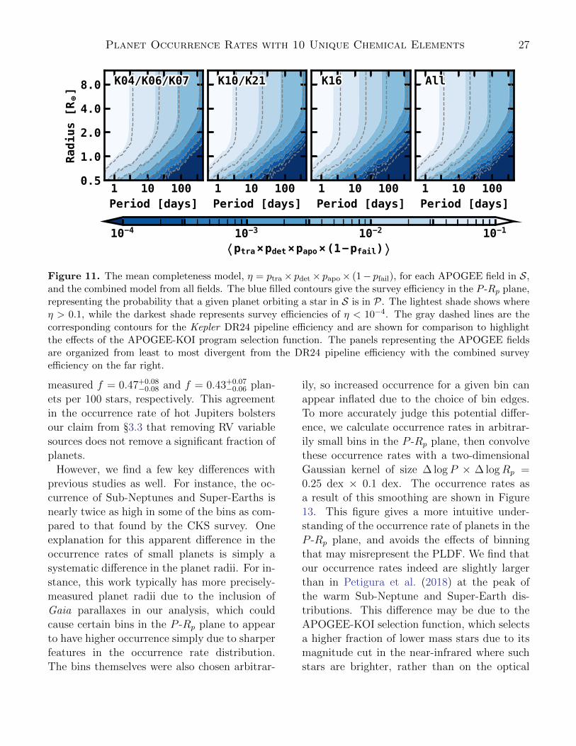

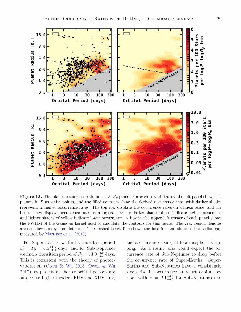


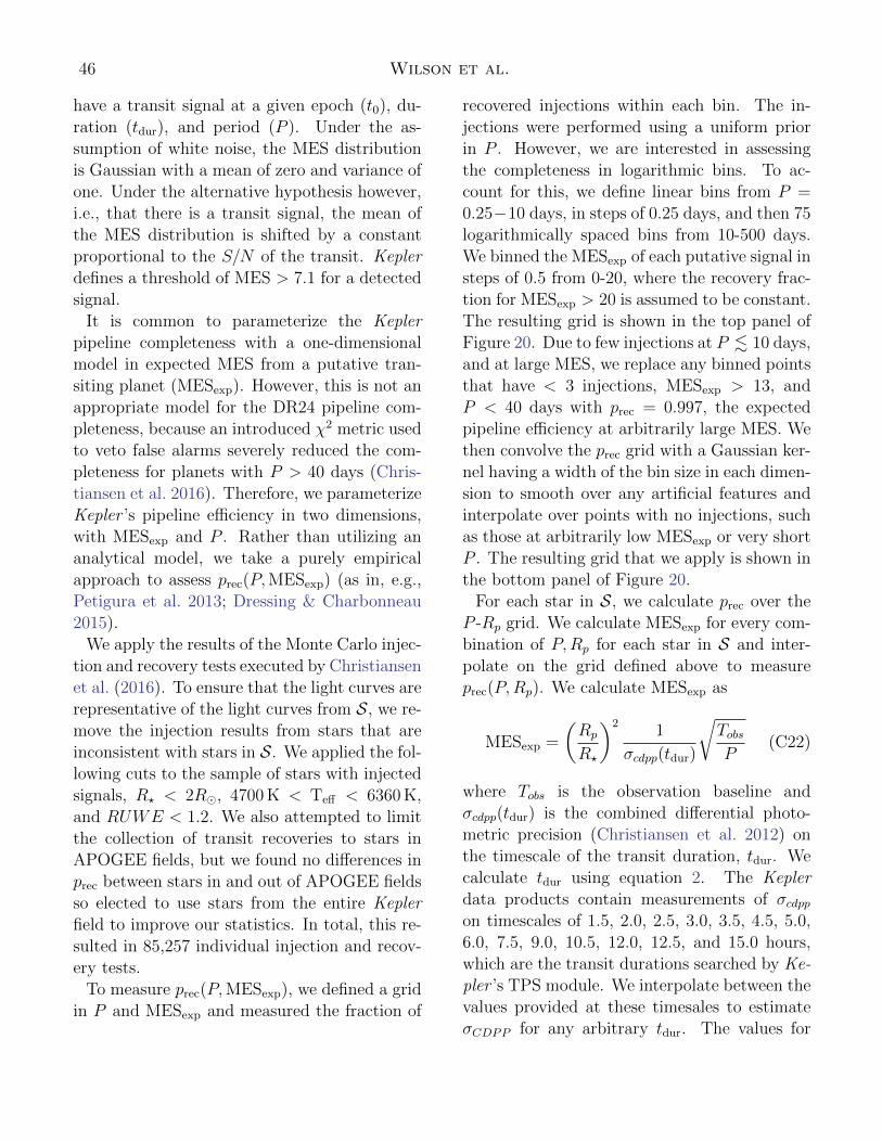

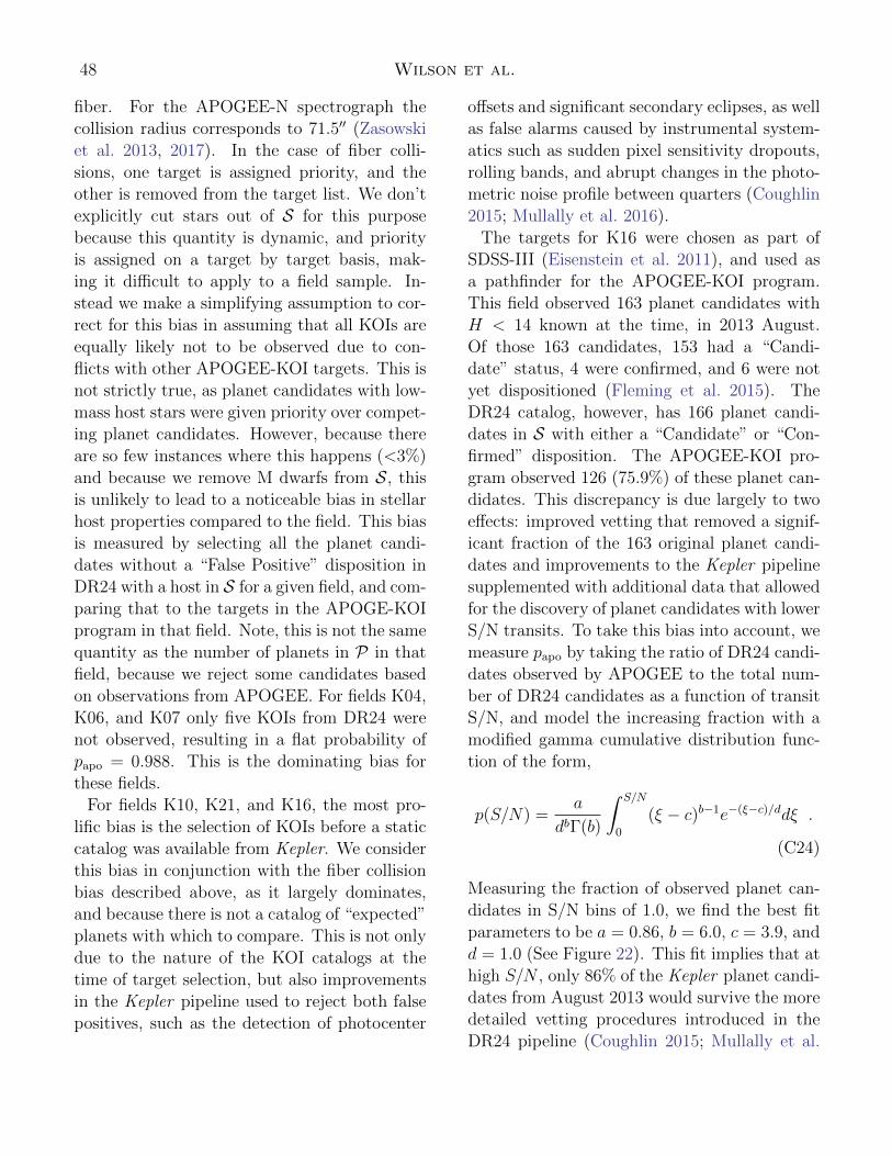
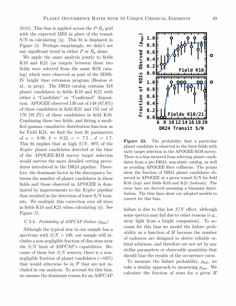
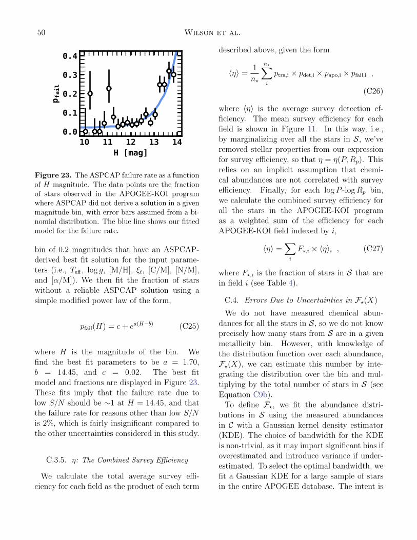


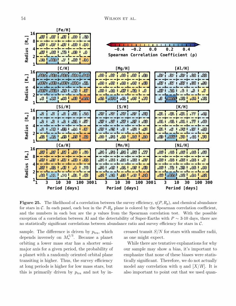


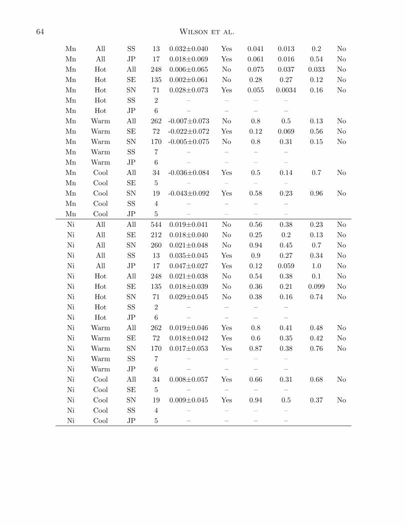


![arXiv:1903.08832v2 [astro-ph.IM] 28 Aug 2019draft version august 29, 2019 typeset using latex twocolumn style in aastex63 eht-hops pipeline for millimeter vlbi data reduction lindy](https://static.documents.pub/doc/80x56/607d88ba8e2b932de15ab57d/arxiv190308832v2-astro-phim-28-aug-2019-draft-version-august-29-2019-typeset.jpg)


![arXiv:2003.02430v1 [astro-ph.IM] 5 Mar 2020 · 2021. 7. 12. · Draft version March 6, 2020 Typeset using LATEX twocolumn style in AASTeX63 Accurate Machine Learning Atmospheric Retrieval](https://static.documents.pub/doc/80x56/6149b8a412c9616cbc68f213/arxiv200302430v1-astro-phim-5-mar-2020-2021-7-12-draft-version-march-6.jpg)

![y 5 6, z x arXiv:2003.10451v2 [astro-ph.EP] 29 Apr 2020 · Draft version May 1, 2020 Typeset using LATEX twocolumn style in AASTeX63 The TESS{Keck Survey. I. A Warm Sub-Saturn-mass](https://static.documents.pub/doc/80x56/5eb57665917422096c0ebc08/y-5-6-z-x-arxiv200310451v2-astro-phep-29-apr-2020-draft-version-may-1-2020.jpg)


![arXiv:2001.08227v2 [astro-ph.SR] 11 Jun 2020 · 2020-06-15 · Draft version June 15, 2020 Typeset using LATEX twocolumn style in AASTeX63 Abundances in the Milky Way across ve nucleosynthetic](https://static.documents.pub/doc/80x56/5f09fbd27e708231d42972d9/arxiv200108227v2-astro-phsr-11-jun-2020-2020-06-15-draft-version-june-15.jpg)


![arXiv:2006.14670v1 [astro-ph.EP] 25 Jun 2020 · 2020-06-29 · Draft version June 29, 2020 Typeset using LATEX default style in AASTeX63 Titan in Transit: Ultraviolet Occultation](https://static.documents.pub/doc/80x56/5f59f7e4e9785a07c917d180/arxiv200614670v1-astro-phep-25-jun-2020-2020-06-29-draft-version-june-29.jpg)

![arXiv:1912.05556v2 [astro-ph.EP] 26 Jan 2020arXiv:1912.05556v2 [astro-ph.EP] 26 Jan 2020,,,Draft version January 28, 2020 Typeset using LATEX twocolumnstyle in AASTeX63 GJ 1252 b:](https://static.documents.pub/doc/80x56/5e5cd0274e01f3532d3b3a87/arxiv191205556v2-astro-phep-26-jan-2020-arxiv191205556v2-astro-phep-26.jpg)
