DRAG COEFFICIENT REDUCTION AT VERY HIGH WIND SPEEDS John A.T. Bye 1 and Alastair D. Jenkins 2 (1) School of Earth Sciences, The University of Melbourne, Victoria 3010, Australia (2) Bjerknes Centre for Climate Research, Geophysical Institute, The University of Bergen, Allégaten 70 , 5007 Bergen, Norway Abstract The correct representation of the 10m drag coefficient for momentum (K 10 ) at extreme wind speeds is very important for modeling the development of tropical depressions and may also be relevant to the understanding of other intense marine meteorological phenomena. We present a unified model for K 10 , which takes account of both the wave field and spray production, and asymptotes to the growing wind wave state in the absence of spray. A feature of the results, is the prediction of a broad maximum in K 10 . For a spray velocity of 9 m s -1 , a maximum of K 10 ∼ 2.0 × 10 -3 occurs for a 10 m wind speed, u 10 ∼ 40 m s -1 , in agreement with recent GPS sonde data in tropical cyclones. Thus, K 10 is "capped" at its maximum value for all higher wind speeds expected. The effect of spray is also shown to flatten the sea surface by transferring energy to longer wavelengths. 1
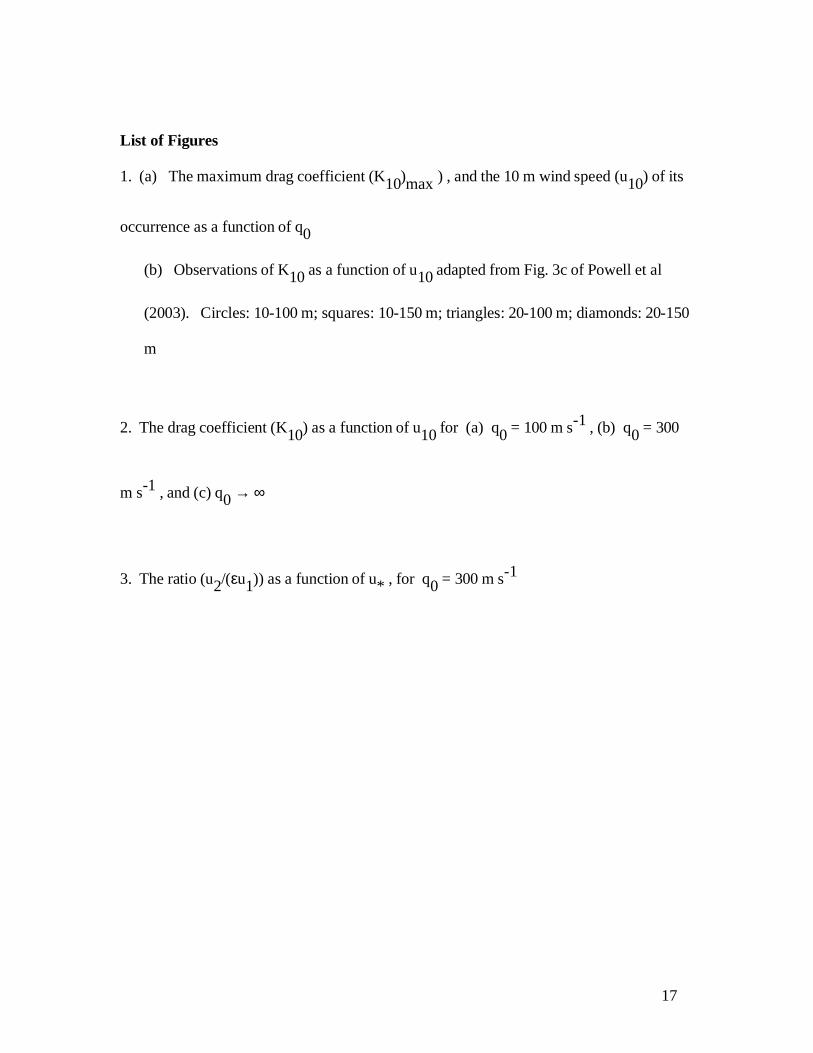
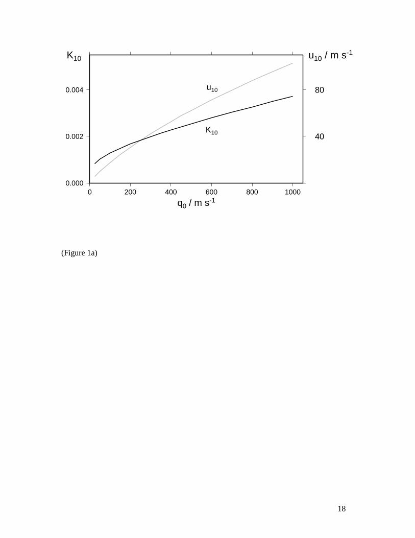
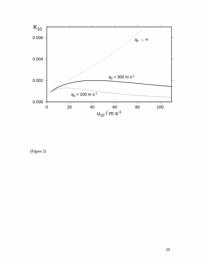
Transcript
DRAG COEFFICIENT REDUCTION AT VERY HIGH WIND SPEEDS
John A.T. Bye1 and Alastair D. Jenkins2
(1) School of Ear th Sciences, The University of Melbourne, Victor ia 3010, Australia
(2) Bjerknes Centre for Climate Research, Geophysical Institute, The University of
Bergen, Allégaten 70 , 5007 Bergen, Norway
Abstract
The correct representation of the 10m drag coefficient for momentum (K10) at extreme
wind speeds is very important for modeling the development of tropical depressions and
may also be relevant to the understanding of other intense marine meteorological
phenomena. We present a unified model for K10 , which takes account of both the wave
field and spray production, and asymptotes to the growing wind wave state in the absence
of spray. A feature of the results, is the prediction of a broad maximum in K10 . For a
spray velocity of 9 m s-1 , a maximum of K10 ∼ 2.0 × 10⁻³ occurs for a 10 m wind speed,
u10 ∼ 40 m s-1 , in agreement with recent GPS sonde data in tropical cyclones. Thus, K10
is "capped" at its maximum value for all higher wind speeds expected. The effect of
spray is also shown to flatten the sea surface by transferring energy to longer wavelengths.
1
1. Introduction
It is of importance to be able to accurately parameterize air-sea exchange processes at
extreme wind speeds in order to understand the mechanisms which control the evolution of
tropical cyclones (Emanuel, 2003). There are also indications that rapid increases in wind
speed may tend to depress the height of surface waves and thus perhaps reduce the drag
coefficient by the flattening of sea-surface roughness elements (Jenkins, 2001). Here, we
consider momentum exchange, and present a seamless formulation which predicts the drag
coefficient over the complete range of wind speeds. An important aspect of the physics is
the momentum used in the production of spray. The results are calibrated against the
data set of Powell et al (2003), obtained by Global Positioning System dropwind-sonde
(GPS sonde) releases in tropical cyclones .
The basis of the analysis is to apply a general expression for the drag coefficient ( K10 ),
that has been derived from the inertial coupling relations (Bye, 1995), which take account
of the wave field (Bye et al, 2001), to the wave boundary layer (Bye, 1988) in the situation
occurring under hurricane winds, when spray plays a significant role in the air-sea
momentum transfer. The inertial coupling relation may be regarded as a parameterization
of the of the dynamical effect of ocean waves within the coupled system containing the
atmospheric and oceanic near-surface turbulent boundary layers (Jenkins 1989, 1992).
We will outline the derivation of the general expression for the drag coefficient, and then
introduce a simple formulation, which takes account of spray production.
2. A general expression for the 10m drag coefficient ( K10 )
In the wave boundary layer (Bye, 1988),
2
u10 = u1 − u* /κ ln ( zB/10 ) (1)
in which u10 is the wind velocity at 10 m, and u1 is the wind velocity at the height, zB =
1/(2 k0) where k0 is the peak wavenumber of the wave spectrum (which will be called
the surface wind), u* is the friction velocity and κ is von Karman's constant. On
introducing the inertial coupling relationships (Bye, 1995) in which,
u* = KI1/2 ( u1 − u2 / ε ) (2)
and
εuL = ½ (εu1 + u2) (3)
where KI is the inertial drag coefficient, ε = (ρ1/ρ2)1/2, in which ρ1 and ρ2 are
respectively the densities of air and water, u2 is the current velocity at the depth, zB
(which will be called the surface current), εuL is the surface Stokes drift velocity, and the
reference velocity has been set equal to zero for convenience, and also the relation (Bye
and Wolff, 2001),
εuL = r (−u2) (4)
which partitions the Stokes shear and the Eulerian shear in the water in the ratio (r), we
obtain the expression,
u1 = R u* / √KI (5)
3
in which R = ½ (1 + 2r)/(1 + r). Hence on substituting for u1 in (1), we obtain,
1/√K10 = R/√KI -1/κ ln (1/ (20 k0) ) (6)
where K10 = u*2/u10
2 . Finally, on substituting into (6), the relation,
c0/u1 = B (7)
where B is the ratio of the phase speed of the peak wave, c0 = (g/k0)1/2 , in which g is
the acceleration of gravity, and the surface wind, we obtain,


![u.s, - dtic.mil · Pr~fi] c drag, absolute ... absolute coefficient GD =D. ' gS' Parasite drag, absolute coefficient CD'=~S ... the cor-responding Reynolds number is 6,865,000) Angle](https://static.documents.pub/doc/80x56/5ae60a187f8b9a8b2b8cb5a4/us-dtic-fi-c-drag-absolute-absolute-coefficient-gd-d-gs-parasite.jpg)


