GIS Ostrava 2012 - Surface models for geosciences January 23. – 25., 2012, Ostrava DRAINAGE AREA ESTIMATION IN PRACTICE, HOW TO TACKLE ARTEFACTS IN REAL WORLD DATA Abdulghani, HASAN 1 , Petter, PILESJÖ 2 , Andreas, PERSSON 2 1 Department of Earth and Ecosystem Sciences, Faculty of science, Lund University, Sölvegatan 12, 22362, Lund, Sweden [email protected]2 GIS Centre, Lund University, Sölvegatan 10, 22362, Lund, Sweden Abstract Large improvements in flow estimation have been made the last decades. However, most, if not all, of the proposed algorithms have been developed and tested on mathematical, or manipulated natural, surfaces. There is an urgent need to develop algorithms dealing with natural artefacts in the landscape, like flat areas and depressions (sinks), caused by man, generalisation (of data type), or by errors in e.g. interpolation. The aim of this study is to present and test practical solutions making it possible to estimate drainage area over natural surfaces with a special focus on sinks and flat areas. Compared to other studies the main contributions of this research are that we have: adapted surface flow routing algorithms over flat areas to multiple flow algorithms, and developed algorithms letting the user decide which sinks to remove, either by beaching or filling. In both cases the user has the possibility to influence the result, by defining breaching points and deciding thresholds regarding area, volume or depth when filling sinks. In this study algorithms making it possible for the user to fill sinks depending on area, depth or volume have been developed. This increases the possibility to separate natural sinks from ones coursed by data or analysis errors. Also an interactive semi-automatic way of breaching break lines in the terrain is presented. This is needed instead of filling sinks caused by man-made artefacts, like road banks and train lines. Existing culverts are then replaced by used defined breach lines. Multiple flow functions to route overland flow over flat surfaces, caused by filled sinks or generalisation, are presented. The flat areas are classif ied as either ‘flow-out’ or ‘flow-in’. Flow-out occurs when one or more cells on the flat area border have an elevation value lower than the flat area cells. A flat area is classified as ‘flow-in’ when all cells on the border of flat area have elevations higher than the flat area cells. These functions, together with the ones for sink removal, are exemplified and tested on real-world data. Results clearly indicate the benefits of the presented algorithms, making it possible to model overland flow and estimate flow accumulation/drainage area continuously in digital elevation models, without imposing vector hydrology covers (streamlines, lakes etc.). Keywords: drainage area, flow accumulation, DEM, multiple flow distribution, flat areas, sinks INTRODUCTION Catchment topography is critical for models of distributed hydrological processes (Quinn, et al. (1991), Seibert, et al. (1997)). Slope controls flow pathways for surface as well as near surface flow, and influences the sub surface flow pattern substantially. The key parameter derived from catchment topography is flow distribution, which tells us how overland flow is distributed over the catchment area. The fact that flow distribution over a land surface is a crucial parameter in hydrological modelling, in combination with available digital data, has rapidly increased the use of Digital Elevation Models (DEM). Modelling has made it possible to estimate flow on each location over a surface, normally by the use of
Transcript
GIS Ostrava 2012 - Surface models for geosciences January 23. – 25., 2012, Ostrava
when creating gridded raster DEMs based on point or line data. Also scale/cell size can cause sinks. If the
resolution in the DEM is relatively low, small streams and channels, transporting water, can be ‘hidden’.
Kenny et al. (2008) highlight the presence of sinks in real world’s data, and also the need for well-functioning
algorithms for sink removal.
The logical way of thinking when carrying out hydrological modelling is that sinks should not be removed (by
filling or breaching) unless we are sure that they are non-natural artefacts. However, depending on the size
of the sink there might be good reasons to assume that also natural sinks are directly linked to the down-hill
drainage areas, through e.g. wetlands. If so, also some of the natural sinks should be removed.
Sinks need to be filled in order to estimate flow directions from all cells and connects them into flow
distribution and flow accumulation. It should be noted that any unfilled sink will result in stopping flow at that
cell. Sometimes this is not desirable.
Based on the discussion about natural and non-natural sinks above we can conclude that there often is a
need for sink removal. It would be desirable if the cell removal, additional to other knowledge, could be
based on size and form of the sinks. Area, volume as well as depth of a sink might help the user to decide if
it should be removed or not (see Figure 1). Also the form of the sink can be a help for the user to decide if it
should be removed by filling or breaching /see below).
Figure 1. Examples of different forms and sizes of sinks. These parameters are a help when judging if the
sink is natural or not, as well as if natural sinks should be removed. V = volume, d = depth, and a equals the
area of the sink.
Man-made structures (non-natural break lines)
Many man-made structures disturb or block estimated flow in a DEM. The main reason for this is that e.g.
tunnels and culverts are not captured within the data collection, and thus not included in the terrain model. A
DEM covering an area including man-made barriers may thus result in non-natural sinks close to these
structures. The barriers are often roads and railway lines, where structures like culverts, siphons and tunnels
have been ‘hidden’ when constructing the DEM. The resulting sinks should be removed since, in these
cases, all cells are actually connected and the flow should continue through the man-made artefact. It is thus
crucial to identify cells on both ‘sides’ of the artefact, and let water flow between these points e.g. by
breaching the barrier. Such connecting flow structures cannot be detected in the data when creating DEMs.
d
d
d
a
V
a
V
a
V
V
V
GIS Ostrava 2012 - Surface models for geosciences January 23. – 25., 2012, Ostrava
Therefore, it’s crucial to find solution how to handle this before estimating flow, flow accumulation and
drainage area from a DEM.
Flat areas
A flat area cell can be defined as a cell surrounded by one or more cells with the same elevation, and no cell
with lower elevation (see Figure 2). Flat cells do not exist in the reality, but sometimes in DEMs depending
on generalisation of data type (maybe only integer is used, or a limited number of decimals) as well as filled
sinks. This implies that flow should be modelled over flat areas, also justified by the fact that water flows over
flat areas due to the change in the energy when water is accumulated (depth increases). Water naturally
always flows to places with lower elevation, even if the terrain is ‘terraced’.
The question is of course how flow should be modelled over these flat areas. The flow can be defined as
either ‘flow-out’ or ‘flow-in’. Flow-out implies that the flow from the flat area cells is directed out of the flat
area, while flow-in occurs when the flow is converging in the centre of the flat area. The cell in the centre of
the flat area will then have no flow out, and is treated as a sink.
Figure 2. A 3 by 3 cell window exemplifying a flat area cell (the centre cell). The flat cell is surrounded by one
or many cells with the same elevation, and no cells with lower elevation. Flow from a flat cell can be none, or
outflow to one or more of the neighbouring cells with same elevation.
AIM
It is a fact that the presence of sinks, man-made structures, as well as flat areas in digital elevation models,
does course great difficulties in hydrological modelling. No operational solutions how to tackle these
problems in combination with a multiple flow routing algorithm have yet been presented.
The aim of this study is to develop, present and test practical solutions making it possible to estimate flow
accumulation/drainage area over natural surfaces, represented as gridded raster DEMs, in an effective and
usable way. The solutions will be applied on a real-world data set in order to exemplify their effects and
usability.
METHODOLOGY
Below follows a step-by-step description of how to tackle the above-mentioned artefacts in real world data.
All software referred to is available through www.gis.lu.se/petter.
Cell classification
In order to separate and deal with the artefacts in the real-world DEMs we decided to label/classify all cells in
the DEM. Three different classes were used, namely ‘Flat’, ‘Sink’, or ‘Undisturbed’ cells. Figure 3 is
illustrating the different classes using a 3 by 3 cell window.
In a 3 by 3 window, the centre cell is classified as flat if at least one of the eight surrounding cells has the
same elevation as the centre cell, while all other cells have a higher elevation value (see Fig. 3a). A flat area
is a group of cells consisting of at least two flat cells neighbouring each other. A cell is classified as sink
10
10 12 10
10
12 10 12
12
GIS Ostrava 2012 - Surface models for geosciences January 23. – 25., 2012, Ostrava
when all its neighbours have higher elevations (see Fig. 3b), while all remaining cells, having at least one cell
with a lower elevation value are classified as undisturbed (see Fig 3c).
Figure 3. Illustrations of the different topographic forms classified by the use of a 3 by 3 cell window. A flat
cell (a) is surrounded by cells with equal and higher elevations; a sink cell (b) is surrounded only by cells with
higher elevations, while undisturbed cells (c) are neighboring at least one cell with lower elevation.
Filling sinks
As stated above some sinks in the DEM data might be a result of man-made artefacts, and need to be
removed. In order to do this, and also include flexibility regarding area, depth and volume of the sink, a
function was created in MATLAB (MathWorks (2008)). This function, attached in Appendix 1, makes it
possible for the use to select threshold values (area, depth and volume) for sink removal through filling.
The idea behind the function is rather straight forward; Elevation values in flat areas (consisting of
neighbouring cells classified as flat, see above) are compared to the elevation value of the lowest adjacent
‘non-flat area’ cell. The number of cells in the flat area multiplied by the cell size equals the area, the
maximum difference in elevation equals the depth of the sink, and the sum of all differences in elevation
multiplied by the cell size equals the volume.
The user is presented statistics (area, depth and volume) of the sinks, and then has the possibility to
eliminate sinks of decided form and size by filling. The function also makes it possible to identify sinks to be
removed by breaching (see Section Breaching break lines below).
Breaching break lines
If we know that man-mad artefacts, like roads, train lines or other walls are present in the data or suspected
by visual interpretation of the DEM or analysis of the form and sizes of sinks (see above) there is a need for
breaching of these artefacts. Thus a function (see Appendix 2) to breach the cells was added, in order to
enable users to deal with e.g. man-made flow barriers like roads and railway lines or any other type of break
lines. This function breaches the barrier by connecting two user-defined points/cells on the opposite sides of
the obstruction. This is done in a semi-automatic way, where the user selects the approximate location of the
two end points of the breach line, and the program searches and proposes suitable points/cells (to be
confirmed or changed by the user). Rules used to propose these points are that, the starting point (higher
elevation) should be the lowest point on the up-slope side of the barrier and higher than the end point, being
the highest point on the other side of the barrier. When the points are selected the elevation of all cells in
between the points will be changed according to a linear regression line between the points. The function as
2 363
5 6
73 4
75 5
6 5 5
7 6 7
13 2
3
7
2
1 31
(c) Undisturbed
(a) Flat (b) Sink
GIS Ostrava 2012 - Surface models for geosciences January 23. – 25., 2012, Ostrava
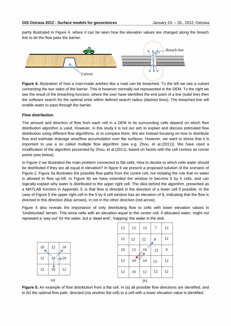
partly illustrated in Figure 4, where it can be seen how the elevation values are changed along the breach
line to let the flow pass the barrier.
Figure 4. Illustration of how a man-made artefact like a road can be breached. To the left we see a culvert
connecting the two sides of the barrier. This is however normally not represented in the DEM. To the right we
see the result of the breaching function, where the user have identified the end point of a line (solid line) then
the software search for the optimal ends within defined search radius (dashed lines). The breached line will
enable water to pass through the barrier.
Flow distribution
The amount and direction of flow from each cell in a DEM to its surrounding cells depend on which flow
distribution algorithm is used. However, in this study it is not our aim to explain and discuss estimated flow
distribution using different flow algorithms, or to compare them. We are instead focusing on how to distribute
flow and estimate drainage area/flow accumulation over flat surfaces. However, we want to stress that it is
important to use a so called multiple flow algorithm (see e.g. Zhou, et al.(2011)). We have used a
modification of the algorithm presented by Zhou, et al.(2011), based on facets with the cell centres as corner
points (see below).
In Figure 2 we illustrated the main problem connected to flat cells; How to decide to which cells water should
be distributed if they are all equal in elevation? In figure 5 we present a proposed solution of the scenario of
Figure 2. Figure 5a illustrates the possible flow paths from the centre cell, not violating the rule that no water
is allowed to flow up-hill. In Figure 5b we have extended the window to become 5 by 5 cells, and can
logically explain why water is distributed to the upper right cell. The idea behind the algorithm, presented as
a MATLAB function in Appendix 3, is that flow is directed in the direction of a lower cell if possible. In the
case of Figure 5 the upper right cell in the 5 by 5 cell window has an elevation of 8, indicating that the flow is
directed in this direction (blue arrows), in not in the other direction (red arrow).
Figure 5 also reveals the importance of only distributing flow to cells with lower elevation values in
‘Undisturbed’ terrain. This since cells with an elevation equal to the centre cell, if allocated water, might not
represent a ‘way out’ for the water, but a ‘dead end’, ‘trapping’ the water in the sink.
Figure 5. An example of flow distribution from a flat cell. In (a) all possible flow directions are identified, and
in (b) the optimal flow path, directed (via another flat cell) to a cell with a lower elevation value is identified.
10
10 12 10
10
12 10 12
12
Culvert
(b) (a)
Breach line
12 12 8
12
12 10
10 12 10
10
12 10 12
12
12 12 12 7 12
12
9
12
12 12
12
GIS Ostrava 2012 - Surface models for geosciences January 23. – 25., 2012, Ostrava
Two different functions has been developed and added to the main flow distribution program in order to
handle flow over flat areas. The functions are attached in Appendix 3 and 4.
FLAT_Flow_out function (see Appendix 3) is a function directing the flow from flat cells where a way out of
the flat area can be found. Examples are illustrated in Figure 5 above and Figure 6 below. Estimating the
flow directions is done according to the following steps:
1. Identify outlets, i.e. cells just outside the border of the flat area with elevation values less than the flat
area.
2. Assign neighbouring flat cells flow directions pointing at the outlet cells (by vector addition and splitting,
see below).
3. Assign neighbouring flat cells flow directions pointing at the cells assigned in step 2.
4. Continue like above until all flat cells have been assigned flow directions.
So, the procedure starts by giving neighbouring cells to the ‘out flow’ cell flow directions ‘pointing’ to that cell,
and then stepwise move further and further away from the out flow cell assigning flat cells flow directions to
neighbours with a defined direction. Cells with the highest number of neighbours with defined flow directions
are processed first, followed by cells with lower numbers of “defined neighbours”.
The flow routing from a flat cell is done by vector addition. Since we are using a multiple flow algorithm a
non-flat cell normally distributes water to more than one neighbouring cell. The flow distribution can be
described as vectors in different directions (maximum eight, equivalent to the directions to the eight
neighbour cells), where each vector has a length corresponding to the amount of water directed in that
direction (0 – 100%). By adding all these vectors for all non-flat neighbour cells (maximum eight neighbor
cells with maximum eight vectors each) a new vector is created (see Pilesjö, et al. (1998)). This vector is
supposed to represent the flow from the flat cell. Normally the direction of this vector falls in between to
neighbouring cells. If so it is split proportionally (see Pilesjö, et al. (1998)), resulting in multiple flow also over
flat areas.
The FLAT_Flow_in function (see Appendix 4) is used when there is no way out from the flat area. An
example is presented in Figure 6b below. All cells just outside the border of the flat area have elevations
higher than the flat area cells, and this result in a converging flow in the centre. This centre cell will have no
defined flow and will be treated as a sink (see above). The flow directions of the surrounding cells will be
estimated (by vector addition) starting from the flat cells that have the maximum number of known distributed
flow directions cells (i.e. the border cells of the flat area).
Figure 6. Illustrations how flow distribution is assigned to cells in two different types of flat areas. In example
(a) the flat area has two outflow cells, resulting in a continuous flow pattern from the centre of the flat area,
while in (b) the flat area has no outflow, resulting in a sink (or actually a cell treated as a sink) in the middle
of the flat area.
As mentioned above, estimated flow directions from undisturbed cells will be dependent on the used
algorithm. In our study, we have used a development of a facet-based algorithm presented by (Zhou, et al.
(2011)).
(b) (a)
GIS Ostrava 2012 - Surface models for geosciences January 23. – 25., 2012, Ostrava
Above we have discussed flow distribution over flat areas. If an area is undisturbed, there are a large
number of flow algorithms to choose between (see e.g. O'Callaghan, et al. (1984), Holmgren (1994), Mark
(1984), Freeman (1991), Pilesjö, et al. (1998)), all capable of estimating water flow. We have used an
improved version of the facet-based presented in (Zhou, et al. (2011)). This method starts by creating
triangular facets around centre cells in 3 by 3 cell windows in the regular gridded DEM (see Figure 7).On
these eight facets water flow is modelled by using slope and slope direction of each facet. Incoming (from
other cells/facets) as well as produced (precipitation) water is tracked over a facet, all the way to the facet
border where it enters another facet.
Figure 7. In the used flow distribution algorithm facets are created around each centre cell. The slopes and
slope directions of these facets are used to track the theoretical water flow, and estimate to which
neighboring cell/cells water will be transported.
It should be noted that, independently of flow algorithm, estimated flow from sink cells is estimated to zero.
This means that an unfilled sink interrupts the flow pattern within the DEM, creating an isolated drainage
area
Flow accumulation/Drainage area
In order to estimate flow accumulation (often referred to as drainage area) the drainage paths over the
surface have to be traced, and the number of up-slope cells (area) transporting water to each and every cell
has to be calculated. This is normally (see Oimoen (2000), Lindsay, et al. (2005), Band (1986), Beven, et al.
(1979), Jenson, et al. (1988)) done by starting a ‘search function’ from peak cells, only transporting water to
surrounding cells but not receiving water from neighbour cells. The drainage area for these peak cells will be
one cell, and the drainage areas for the down-slope neighbour cells that they are transporting water to will be
proportionally updated. For example, if water is transported to two neighbour cells on an equal basis both
these cells will get an updated drainage area of +0.5. Then these peak cells are flagged as visited, and be
neglected in further processing. After this the software will again search for cells with only out flow. Since the
original peaks are excluded this will be cells neighbouring the peaks. Flow to down-slope neighbouring cells
will be estimated, and then next iteration will start one ‘level’ down. This continues until all cells have been
examined. A detailed description of the estimation of flow accumulation can be found in (Pilesjö, et al.
(1998)). The method is equivalent to counting the flow paths/flow packages in the parts of the eight facets
covering the centre cell (see Figure 7).
EXPERIMENT
The proposed methods have been tested using real-world data. The newly developed drainage area
algorithms focusing on sink removal and flow estimation on flat areas have been applied to a real-world
DEM, and the effects have been studied and compared. The spatial pattern of derived flow distribution is
visually examined to detect significant artefacts.
1 2
3 4 5
6
7 8
C1 C2
M
GIS Ostrava 2012 - Surface models for geosciences January 23. – 25., 2012, Ostrava
Real-World DEM
The real-world earth surface elevation data used are from the Stordalen mire and its catchment area.
Stordalen is a peatland area in the Arctic region, 10 km west of Abisko (68º 20' N, 19º 03' E) in northern
Sweden. The Stordalen mire is a very flat area with many ponds and water bodies, resulting in a large
number of flat areas and sinks. Moreover, a road and a railway line are constructed in this area, with many
culverts to connect the flow of water between the two sides of the road or the two sides of the railway line.
This site was thus judged as suitable for testing of the new methods dealing with flat areas, sinks and
culverts.
An airborne LiDAR device has been used to measure the surface elevation. LiDAR is an acronym for “Light
Detection And Ranging”, and is a laser-based, remote sensing system used to collect various kinds of
environmental data, including topographic data (Fowler (2001)). Over the area defined above the total
number of measured elevation data points (the raw data) is 76 940 341. This results in a high resolution data
set with an average spatial distribution of approximately 13 points/m2. The LiDAR data in the present study
were retrieved with a TOPEYE S/N 425 system mounted on Helicopter SE-HJC. The altitude when sampling
was 500 m. The LiDAR data have been post processed and adjusted against 54 known points connected to
the national geodetic network. The mean vertical error after post-processing corrections is +0.004 m and the
average magnitude of errors is 0.022 m. The RMSE is 0.031 m and the standard deviation is 0.031 m. For
more details see (Hasan, et al. (2011)).
The raw LiDAR data were interpolated into a raster DEM by using inverse distance interpolation (Shepard
(1968)). An accuracy assessment has been conducted by Hasan et al. (2011) on the created DEMs to find
the best combination of Search radius and cell size. The selected optimum search radius was set to 1 m and
the cell size set to 1 m also (see Hasan et al. (2011)). The DEM is presented in Figure 8 below.
Figure 8. Hill-shade of the used DEM covering the Stordalen area in northern Sweden.
RESULTS
Figure 9a shows the sinks in the real-world DEM while Figure 9b shows the remain sinks after breaching all
man-made structures using the culvert breaching approach presented in this study. Large sinks are removed
GIS Ostrava 2012 - Surface models for geosciences January 23. – 25., 2012, Ostrava
by breaching few cells. Referring to Figure 9 one can clearly identify the problem with a large number of
sinks, which would heavily influence estimated drainage area if not removed.
Figure 9a and 9b. Figure 9a illustrates the sinks (coloured red) in the Stordalen area. Figure 9b illustrates
the remain sinks after breaching all man-made structures with the culvert approached presented in this
study.
Figure 10 a-d shows show estimated drainage area, using two different algorithms and two different zooming
views. In Figure 10a and figure 10b the single flow D8 algorithm (Jenson, et al. (1988)) has been applied,
while the result of the newly developed algorithms presented in this paper is illustrated in Figure 10c and
10d.
Figure 10a-d. Shows estimated drainage area, using two different algorithms and two different zooming
views. In Figure 10a and Figure 10b the single flow D8 algorithm (Jenson, et al. (1988)) has been applied,
while the result of the newly developed algorithms presented in this paper is illustrated in Figure 10c and
10d.
a b
a b
c d
GIS Ostrava 2012 - Surface models for geosciences January 23. – 25., 2012, Ostrava
In Figure 11 we see the effect of breaching a barrier. A sink created by a train line is filled, and the resulting
drainage area estimation is presented in Figure 11a. If, instead of filling the sink, the barrier (in this case the
train line) is breached a totally different flow and drainage area pattern is created (Figure 11b). This
highlights the importance of flexibility and choice in sink removal, made possible by the introduction of the
above-mentioned algorithms.
Figure 11. Illustrations of the result of using and not using the function to breach barriers and connect the
flow between two sides of a barrier, in this case a railway line. In figure 11a (left) the sink has been filled, and
the flow accumulation/drainage area has been estimated. This results in a large area of ‘regular’ flow. In
Figure 11b (right) a few cells in the barrier have been breached, resulting in a more ‘natural’ estimated flow.
DISCUSSION AND CONCLUSIONS
In this research paper we have presented new and modified solutions for surface water routing based on a
digital elevation model (DEM). These include different ways of sink removal, as well as water routing over flat
surfaces. The related problems are not at all new, but have been discussed by several authors during the
last decades (see e.g. Oimoen (2000), Lindsay, et al. (2005), Beven, et al. (1979), Jenson, et al. (1988) and
Kenny, et al. (2008)). Our contributions to the discussions and solutions are mainly that:
Our solutions are designed to be applied in combination with multiple flow algorithms, proved to be
superior to the “normally used” single flow approach (see e.g. Zhou, et al. (2011)).
We allow the user to interactively choose which sinks that should be filled or breached.
We allow the user to interactively set thresholds for sinks to be filled, referring to sink area, sink volume,
and sink depth.
We allow the user to interactively define points/cells to breach barriers.
We are only using the DEM for the flow routing, and no vector layers, like streams and lakes are
needed.
It should also be noted that elevation (cell) values are not automatically updated, but the user is given the
option to keep the original values, in order not to disturb e.g. estimations of slope and aspect.
It is well known that multiple flow algorithms are more realistic than e.g. the D8 solution (O'Callaghan, et al.
(1984)). Thus, multiple flows over flat areas are logical. By summarizing the flow vectors (in different
directions) of neighbouring cells, with defined flows, around a flat cell, and then split the summarized vector
into two adjacent cells, a more realistic flow is modelled.
The question of which sinks that is results of errors and/or generalization is almost impossible to reply.
However, by letting the user decide this, based on expert knowledge and/or visual interpretation of the DEM,
a b
GIS Ostrava 2012 - Surface models for geosciences January 23. – 25., 2012, Ostrava
and define thresholds for the area, volume or depth of these, we might get a more realistic representation of
the reality after a sink removal.
The proposed culvert function can be cost effective. Breaching a few cells representing e.g. a culvert costs
less than filling a large area around the sink. Moreover the culvert function can be used by civil engineers to
help select the best locations for constructing culverts, tunnels or siphons.
We suggest that the methods presented in this paper are used together with other solutions, e.g. breaching
according to (Garbrecht, et al. (1999)), and sink flow routing according to Seibert et al. (2007). Seibert et al.
(2007) present an “elegant solution”, where flow from a sink is transported as subsurface flow until it reaches
the closest cell with a lower elevation than the sink bottom. From there the flow continues on the surface. Of
course the results will also improve if methods like the one presented by Kenny, et al. (2008), including
vector features if streams, lakes etc., will be used. However, integration of these methods can be time
consuming, and they should preferably be adapted to multiple flow solutions of surface flow routing.
When estimating flow accumulation/drainage area and wetness index in order to increase accuracy in e.g.
carbon modelling, data are often relatively course and generalized (see e.g. Hasan, et al. (2011)). Detailed
stream networks are seldom available and the users have to rely on the DEM only. Under such
circumstances the methods presented above are very useful.
REFERENCES
Quinn, P., K. Beven, P. Chevallier and O. Planchon. (1991) The prediction of hillslope flow paths for distributed hydrological modelling using digital terrain models. Hydrological Processes, 5, 59-79.
Seibert, J., K. H. Bishop and L. Nyberg. (1997) A test of TOPMODEL's ability to predict spatially distributed groundwater levels. Hydrological Processes, 11, 1131-1144.
Zhou, Q., P. Pilesjö and Y. Chen. (2011) Estimating surface flow paths on a digital elevation model using a triangular facet network. Water Resour. Res., 47, W07522.
Beven, K. J. and I. D. Moore. (1993) Terrain analysis and distributed modelling in hydrology / edited by K.J. Beven and I.D. Moore. Wiley & Sons, Chichester, England ; New York.
Wilson, J. P. and J. C. Gallant. (2000) Terrain Analysis: Principles and Applications. Wiley,
Seibert, J. and B. L. McGlynn. (2007) A new triangular multiple flow direction algorithm for computing upslope areas from gridded digital elevation models. Water Resour. Res., 43, W04501.
Pilesjö, P., Q. Zhou and L. Harrie. (1998) Estimating flow distribution over digital elevation models using a form-based algorithm. Geographic Information Sciences, 4, 44-51.
O'Callaghan, J. F. and D. M. Mark. (1984) The extraction of drainage networks from digital elevation data. Computer Vision, Graphics, and Image Processing, 28, 323-344.
Band, L. E. (1986) Topographic partition of watersheds with digital elevation models. Water Resources Research, 22, 15-24.
ESRI. (1991) Cell-based Modelling with GRID, Environmental System Research Institute.
Mark, D. M. (1984) Automated detection of drainage networks from digital elevation models. Cartographica, 21, 168-178.
Freeman, T. G. (1991) Calculating catchment area with divergent flow based on a regular grid. Computers and Geosciences, 17, 413-422.
Holmgren, P. (1994) Multiple flow direction algorithms for runoff modelling in grid based elevation models: an empirical evaluation. Hydrological Processes, 8, 327-334.
Pilesjö, P. and Q. Zhous, (1996), A multiple flow direction algorithm and its use for hydrological modelling, Geoinformatics´96, West Palm Beach, FL, April 26-28, 366-376.
Wolock, D. M. and G. J. McCabe. (1995) Comparison of single and multiple flow direction algorithms for computing topographic parameters in TOPMODEL. Water Resources Research, 31, 1315-1324.
GIS Ostrava 2012 - Surface models for geosciences January 23. – 25., 2012, Ostrava
Quinn, P. F., K. J. Beven and R. Lamb. (1995) The ln(a/tan-beta) Index - how to calculate it and how to use it within the TOPMODEL framework. Hydrological Processes, 9, 161-182.
Costa-Cabral, M. C. and S. J. Burges. (1994) Digital elevation model networks (DEMON): A model of flow over hillslopes for computation of contributing and dispersal areas. Water Resources Research, 30, 1681-1692.
Fairfield, J. and P. Leymarie. (1991) DRAINAGE NETWORKS FROM GRID DIGITAL ELEVATION MODELS. Water Resources Research, 27, 709-717.
Tarboton, D. G. (1997) A new method for the determination of flow directions and upslope areas in grid DEMs. Water Resources Research, 33, 309-319.
Beven, K. J. and M. J. Kirkby. (1979) A physically based, variable contributing area model of basin hydrology. Hydrological Sciences Journal, 24, 43-69.
Jenson, S. K. and J. O. Domingue. (1988) Extracting topographic structure from digital elevation data for geographic information system analysis. Photogrammetric Engineering and Remote Sensing, 54, 1593-1600.
Kenny, F., B. Matthews and K. Todd. (2008) Routing overland flow through sinks and flats in interpolated raster terrain surfaces. Computers & Geosciences, 34, 1417-1430.
Lindsay, J. B. and I. F. Creed. (2005) Sensitivity of digital landscapes to artifact depressions in remotely-sensed DEMs. Photogrammetric Engineering and Remote Sensing, 71, 1029-1036.
Oimoen, M. J.s, (2000), An effective filter for removal of production artifacts in US Geological Survey 7.5-minute digital elevation models, Proceedings of the 14th International Conference on Applied Geologic Remote Sensing, Las Vegas, NV, USA. Veridian ERIM International, Ann Arbor, MI, pp. 311-319.
Hasan, A., P. Pilesjö and A. Persson. (2011) The use of LiDAR as a data source for digital elevation models - DEM resolution versus accuracy and estimated slope, drainage area and wetness in northern peatlands. Hydrology and Earth System Sciences, discussion paper.
MathWorks. (2008) MATLAB R2008B. R2008B.
Fowler, R. (2001) Topographic Lidar Maune, Digital Elevation Model Technologies And Applications, American Society for Photogrammetry and Remote Sensing, Maryland.
Shepard, D. (1968) A two-dimensional interpolation function for irregularly-spaced data. Proceedings of the 1968 23rd ACM national conference.
Garbrecht, J. and L. W. Martz. (1999) TOPAZ: an automated digital landscape analysis tool for topographic evaluation, drainage identification, watershed segmentation and subcatchment parameterization; TOPAZ overview. United States Department of Agricultural, Agricultural Research Service (USDA-ARS) Publication No. GRL 99-1, Washington, DC, USA, 26pp.
GIS Ostrava 2012 - Surface models for geosciences January 23. – 25., 2012, Ostrava
Appendix 1 function [FilledDEM,MaxFilleddepth] = fillsinksAH(DEM,Maxdepth)
% this function is for filling pits or sinks or topographic depressions