DrillingNotAble (to find )

PreciseLocation ofSolventsPresented By

Dr. Todd Halihan (Oklahoma State University & Aestus, LLC)Stuart W. McDonald, P.E. (Aestus, LLC)

NEWMOA WorkshopCharacterizing Chlorinated Solvent (DNAPL) Sites

September 11, 2007 - Westford Regency, Westford, MA September 12, 2007 - Publick House, Sturbridge, MA

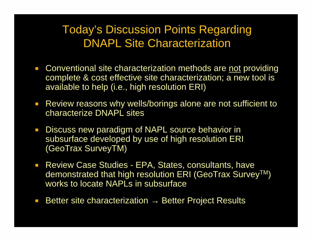
� Conventional site characterization methods are not providing complete & cost effective site characterization; a new tool is available to help (i.e., high resolution ERI)

� Review reasons why wells/borings alone are not sufficient to characterize DNAPL sites

� Discuss new paradigm of NAPL source behavior in subsurface developed by use of high resolution ERI (GeoTrax SurveyTM)

� Review Case Studies - EPA, States, consultants, have demonstrated that high resolution ERI (GeoTrax SurveyTM)works to locate NAPLs in subsurface

� Better site characterization → Better Project Results

Today’s Discussion Points RegardingDNAPL Site Characterization

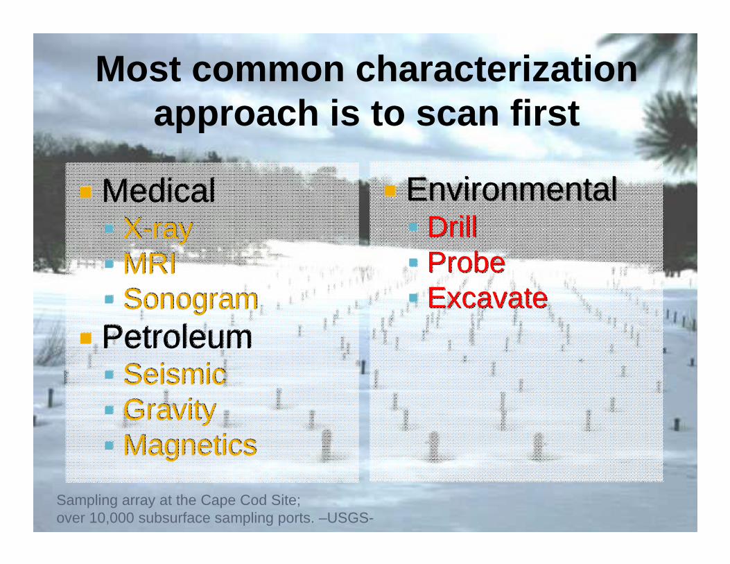
Most common characterization approach is to scan first

� Medical� X-ray� MRI� Sonogram

� Petroleum� Seismic� Gravity� Magnetics

� Environmental� Drill� Probe� Excavate

Sampling array at the Cape Cod Site; over 10,000 subsurface sampling ports. –USGS-

� Medical� X-ray� MRI� Sonogram

� Petroleum� Seismic� Gravity� Magnetics

� Environmental� Drill� Probe� Excavate

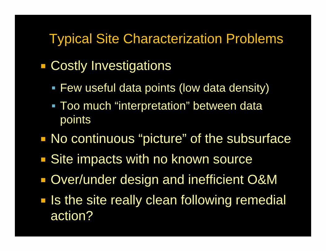
� Costly Investigations

� Few useful data points (low data density)

� Too much “interpretation” between data points

� No continuous “picture” of the subsurface

� Site impacts with no known source

� Over/under design and inefficient O&M

� Is the site really clean following remedial action?

Typical Site Characterization Problems

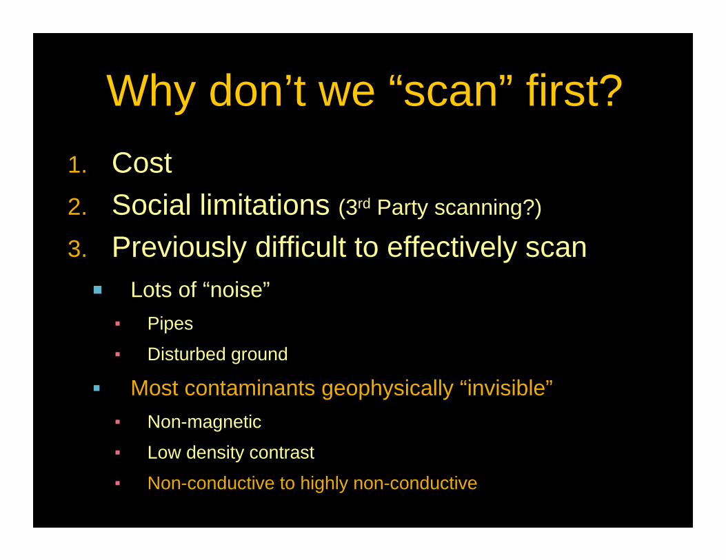
Why don’t we “scan” first?

1. Cost2. Social limitations (3rd Party scanning?)

3. Previously difficult to effectively scan� Lots of “noise”

▪ Pipes

▪ Disturbed ground

� Most contaminants geophysically “invisible”

▪ Non-magnetic

▪ Low density contrast

▪ Non-conductive to highly non-conductive

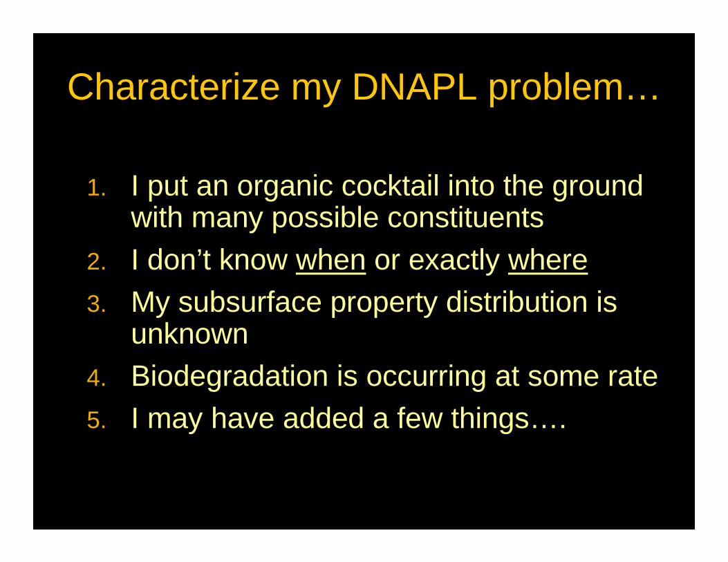
Characterize my DNAPL problem…

1. I put an organic cocktail into the ground with many possible constituents

2. I don’t know when or exactly where3. My subsurface property distribution is

unknown4. Biodegradation is occurring at some rate5. I may have added a few things….

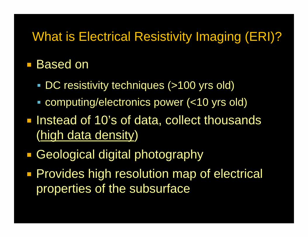
� Based on

� DC resistivity techniques (>100 yrs old)

� computing/electronics power (<10 yrs old)

� Instead of 10’s of data, collect thousands (high data density)

� Geological digital photography

� Provides high resolution map of electrical properties of the subsurface

What is Electrical Resistivity Imaging (ERI)?

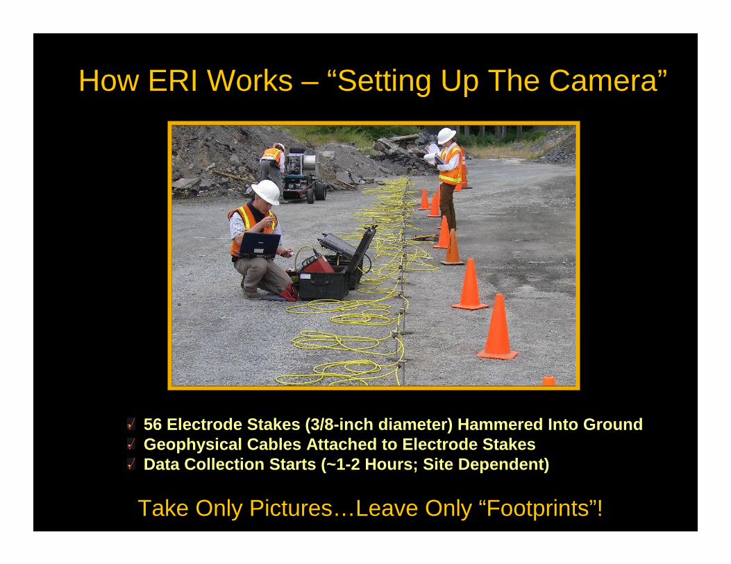
56 Electrode Stakes (3/8-inch diameter) Hammered In to GroundGeophysical Cables Attached to Electrode StakesData Collection Starts (~1-2 Hours; Site Dependent)

How ERI Works – “Setting Up The Camera”

Take Only Pictures…Leave Only “Footprints”!

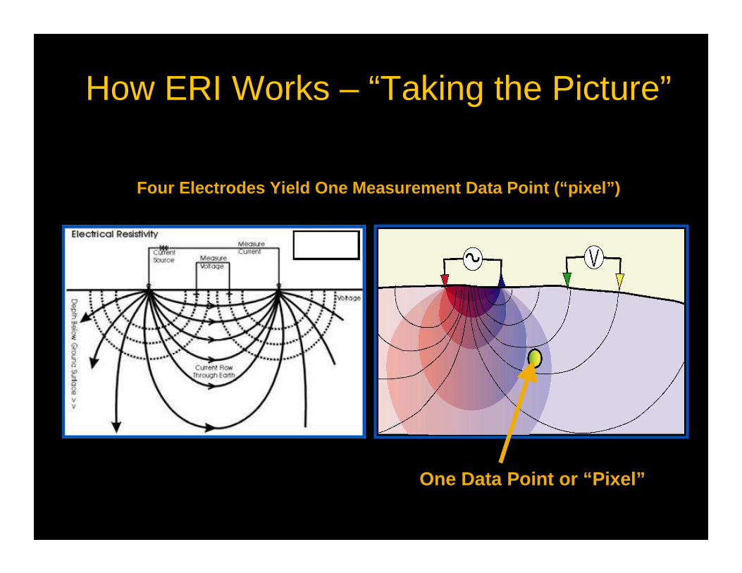
One Data Point or “Pixel”

Four Electrodes Yield One Measurement Data Point (“ pixel”)

How ERI Works – “Taking the Picture”

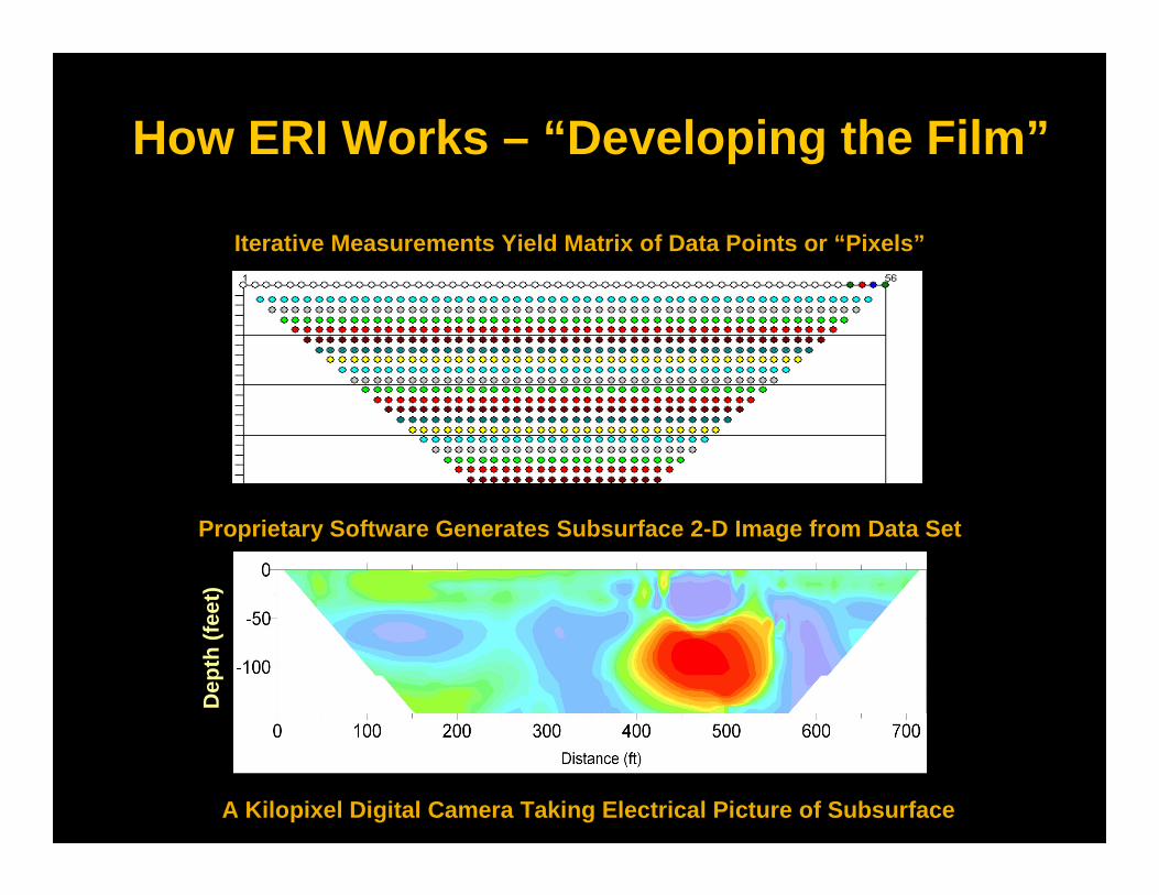
Iterative Measurements Yield Matrix of Data Points o r “Pixels”D

epth

(fe

et)

Proprietary Software Generates Subsurface 2-D Image from Data Set

A Kilopixel Digital Camera Taking Electrical Picture of Subsurface

How ERI Works – “Developing the Film”

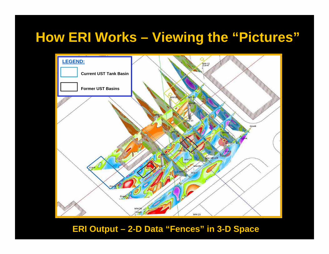
How ERI Works – Viewing the “Pictures”3-D Perspective View - GeoTrax Surveys TM

(From Above and Looking North at All On-Site Surveys)LEGEND:

Current UST Tank Basin

Former UST Basins

ERI Output – 2-D Data “Fences” in 3-D Space

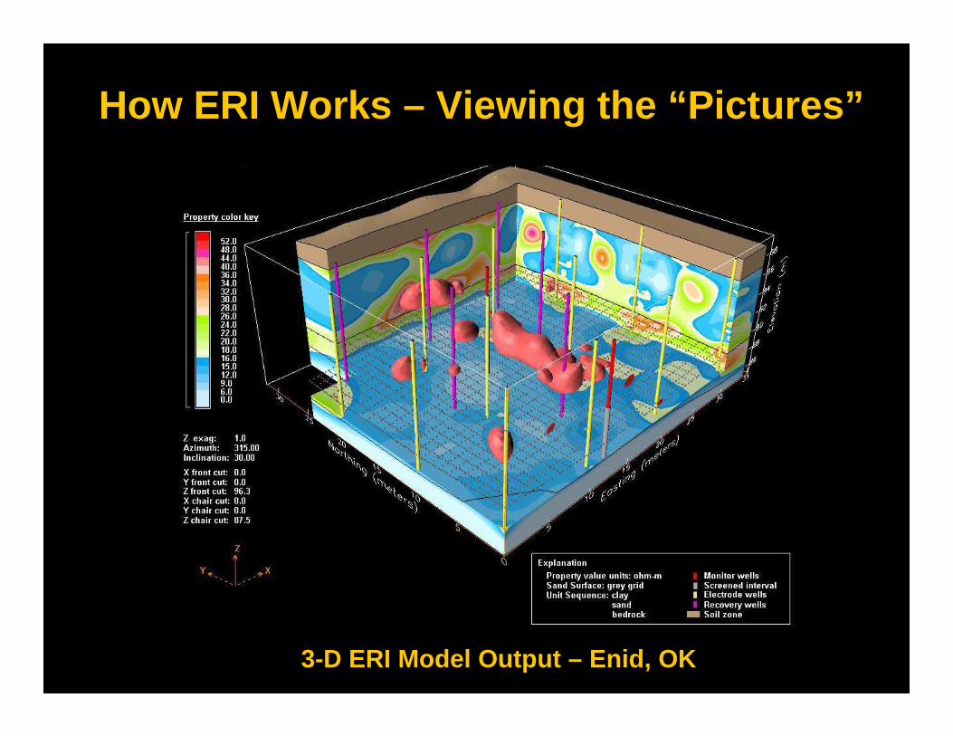
How ERI Works – Viewing the “Pictures”

3-D ERI Model Output – Enid, OK

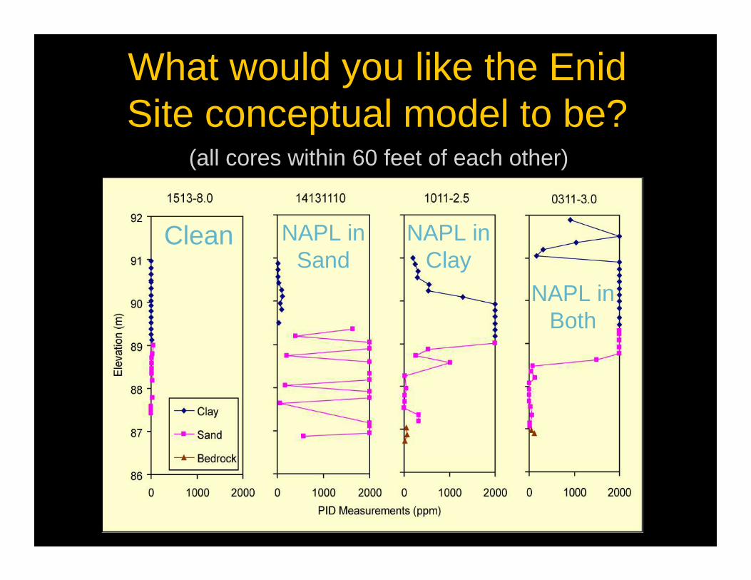
What would you like the Enid Site conceptual model to be?

(all cores within 60 feet of each other)

Clean NAPL inSand

NAPL inClay

NAPL inBoth

Why didn’t we do this before?

Technological Progression

• Data acquisition now 100x faster than 1990

• Data processing now 350x faster than 1990

• Images were not “drillable”

– OSU/Aestus created dramatically improved images– Images can “see” resistive subsurface targets others

can’t

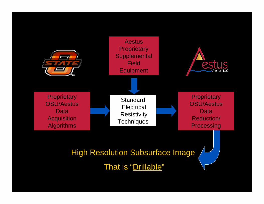
StandardElectricalResistivity

Techniques

ProprietaryOSU/Aestus

DataAcquisitionAlgorithms

AestusProprietary

SupplementalField

Equipment

High Resolution Subsurface Image

That is “Drillable”

ProprietaryOSU/Aestus

DataReduction/Processing

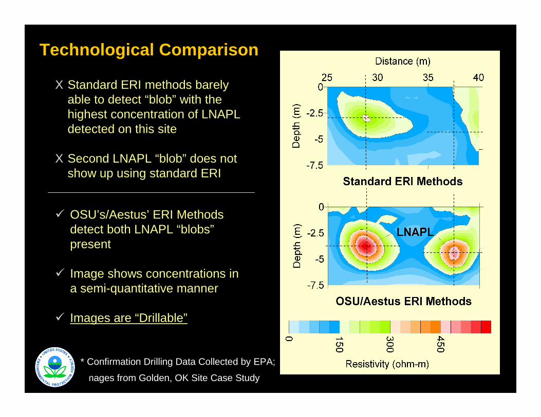
Technological Comparison

Images from Golden, OK Site Case Study

X Standard ERI methods barely able to detect “blob” with the highest concentration of LNAPL detected on this site

X Second LNAPL “blob” does not show up using standard ERI

� OSU’s/Aestus’ ERI Methods detect both LNAPL “blobs”present

� Image shows concentrations in a semi-quantitative manner

� Images are “Drillable”

* Confirmation Drilling Data Collected by EPA;

� Wells do not provide a good estimate of subsurface conditions at DNAPL sites

� No site imaged with this ERI technique has shown a uniform layer with a “thickness” of DNAPL – occurs as discontinuous “blobs”

� Well data should be viewed differently depending on well function, well construction, and whether pre- or post-remediation

Why has it been so hard to understand your site?

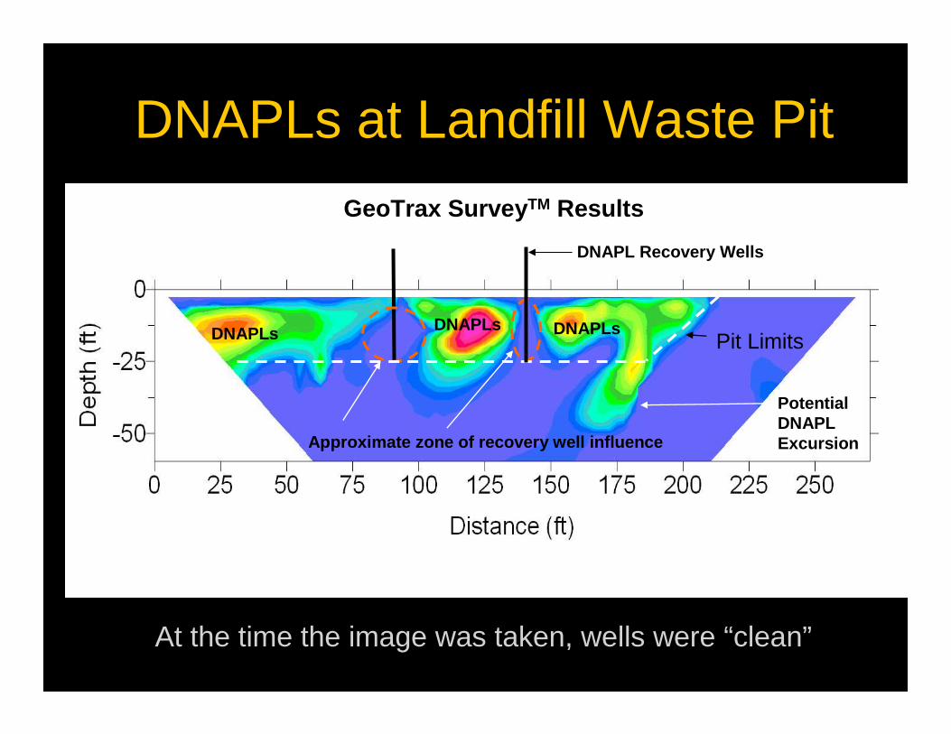
DNAPLs at Landfill Waste Pit

GeoTrax Survey TM Results

DNAPL Recovery Wells

Approximate zone of recovery well influence

PotentialDNAPLExcursion

DNAPLsDNAPLs DNAPLsPit Limits

At the time the image was taken, wells were “clean”

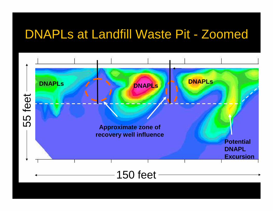
DNAPLs at Landfill Waste Pit - Zoomed

Approximate zone of recovery well influence

PotentialDNAPLExcursion

DNAPLsDNAPLs DNAPLs

150 feet

55 fe

et

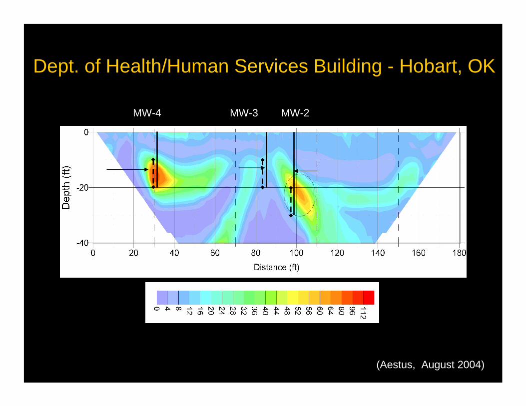
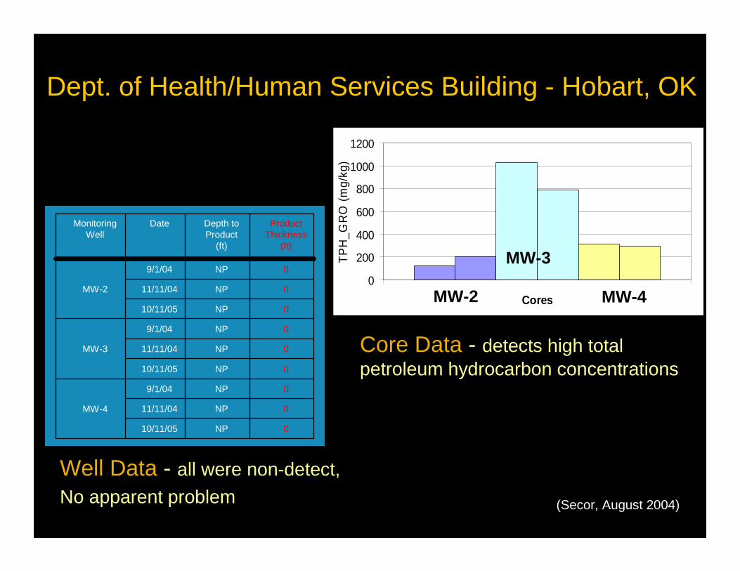
Dept. of Health/Human Services Building - Hobart, OK

MW-4 MW-3 MW-2

(Aestus, August 2004)

(Secor, August 2004)

Core Data - detects high total petroleum hydrocarbon concentrations

Well Data - all were non-detect,

No apparent problem

0NP10/11/05

0NP11/11/04

0NP9/1/04

MW-4

0NP10/11/05

0NP11/11/04

0NP9/1/04

MW-3

0NP10/11/05

0NP11/11/04

0NP9/1/04

MW-2

ProductThickness

(ft)

Depth toProduct

(ft)

DateMonitoringWell

0

200

400

600

800

1000

1200

WellsCores

TP

H_G

RO

(m

g/kg

)

MW-2

MW-3

MW-4

Dept. of Health/Human Services Building - Hobart, OK

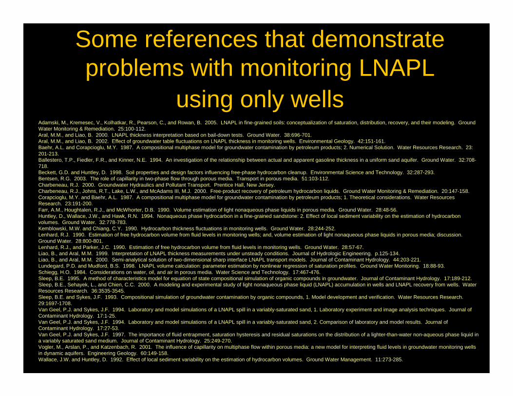
Some references that demonstrate problems with monitoring LNAPL

using only wellsAdamski, M., Kremesec, V., Kolhatkar, R., Pearson, C., and Rowan, B. 2005. LNAPL in fine-grained soils: conceptualization of saturation, distribution, recovery, and their modeling. Ground Water Monitoring & Remediation. 25:100-112.Aral, M.M., and Liao, B. 2000. LNAPL thickness interpretation based on bail-down tests. Ground Water. 38:696-701.Aral, M.M., and Liao, B. 2002. Effect of groundwater table fluctuations on LNAPL thickness in monitoring wells. Environmental Geology. 42:151-161.Baehr, A.L. and Corapcioglu, M.Y. 1987. A compositional multiphase model for groundwater contamination by petroleum products; 2. Numerical Solution. Water Resources Research. 23: 201-213.Ballestero, T.P., Fiedler, F.R., and Kinner, N.E. 1994. An investigation of the relationship between actual and apparent gasoline thickness in a uniform sand aquifer. Ground Water. 32:708-718.Beckett, G.D. and Huntley, D. 1998. Soil properties and design factors influencing free-phase hydrocarbon cleanup. Environmental Science and Technology. 32:287-293.Bentsen, R.G. 2003. The role of capillarity in two-phase flow through porous media. Transport in porous media. 51:103-112.Charbeneau, R.J. 2000. Groundwater Hydraulics and Pollutant Transport. Prentice Hall, New Jersey.Charbeneau, R.J., Johns, R.T., Lake, L.W., and McAdams III, M.J. 2000. Free-product recovery of petroleum hydrocarbon liquids. Ground Water Monitoring & Remediation. 20:147-158.Corapcioglu, M.Y. and Baehr, A.L. 1987. A compositional multiphase model for groundwater contamination by petroleum products; 1. Theoretical considerations. Water Resources Research. 23:191-200.Farr, A.M., Houghtalen, R.J., and McWhorter, D.B. 1990. Volume estimation of light nonaqueous phase liquids in porous media. Ground Water. 28:48-56.Huntley, D., Wallace, J.W., and Hawk, R.N. 1994. Nonaqueous phase hydrocarbon in a fine-grained sandstone: 2. Effect of local sediment variability on the estimation of hydrocarbon volumes. Ground Water. 32:778-783.Kemblowski, M.W. and Chiang, C.Y. 1990. Hydrocarbon thickness fluctuations in monitoring wells. Ground Water. 28:244-252.Lenhard, R.J. 1990. Estimation of free hydrocarbon volume from fluid levels in monitoring wells; and, volume estimation of light nonaqueous phase liquids in porous media; discussion. Ground Water. 28:800-801.Lenhard, R.J., and Parker, J.C. 1990. Estimation of free hydrocarbon volume from fluid levels in monitoring wells. Ground Water. 28:57-67.Liao, B., and Aral, M.M. 1999. Interpretation of LNAPL thickness measurements under unsteady conditions. Journal of Hydrologic Engineering. p.125-134.Liao, B., and Aral, M.M. 2000. Semi-analytical solution of two-dimensional sharp interface LNAPL transport models. Journal of Contaminant Hydrology. 44:203-221. Lundegard, P.D. and Mudford, B.S. 1998. LNAPL volume calculation: parameter estimation by nonlinear regression of saturation profiles. Ground Water Monitoring. 18:88-93.Schiegg, H.O. 1984. Considerations on water, oil, and air in porous media. Water Science and Technology. 17:467-476.Sleep, B.E. 1995. A method of characteristics model for equation of state compositional simulation of organic compounds in groundwater. Journal of Contaminant Hydrology. 17:189-212.Sleep, B.E., Sehayek, L., and Chien, C.C. 2000. A modeling and experimental study of light nonaqueous phase liquid (LNAPL) accumulation in wells and LNAPL recovery from wells. Water Resources Research. 36:3535-3545.Sleep, B.E. and Sykes, J.F. 1993. Compositional simulation of groundwater contamination by organic compounds, 1. Model development and verification. Water Resources Research. 29:1697-1708.Van Geel, P.J. and Sykes, J.F. 1994. Laboratory and model simulations of a LNAPL spill in a variably-saturated sand, 1. Laboratory experiment and image analysis techniques. Journal of Contaminant Hydrology. 17:1-25.Van Geel, P.J. and Sykes, J.F. 1994. Laboratory and model simulations of a LNAPL spill in a variably-saturated sand, 2. Comparison of laboratory and model results. Journal of Contaminant Hydrology. 17:27-53.Van Geel, P.J. and Sykes, J.F. 1997. The importance of fluid entrapment, saturation hysteresis and residual saturations on the distribution of a lighter-than-water non-aqueous phase liquid in a variably saturated sand medium. Journal of Contaminant Hydrology. 25:249-270.Vogler, M., Arslan, P., and Katzenbach, R. 2001. The influence of capillarity on multiphase flow within porous media: a new model for interpreting fluid levels in groundwater monitoring wells in dynamic aquifers. Engineering Geology. 60:149-158.Wallace, J.W. and Huntley, D. 1992. Effect of local sediment variability on the estimation of hydrocarbon volumes. Ground Water Management. 11:273-285.

Now, in general…� Wells provide a limited picture of the subsurface

� ERI provides a great tool to allow sites to be better characterized; ERI is not a magic bullet as confirmation data is required to calibrate images

� Because DNAPL distribution is discontinuous, the total volume estimated using ERI is typically much less than estimates using only well data

� Visual tools provide increased ability to understand sites and communicate to project stakeholders

Why do you need confirmation borings?

� Every site is different- there are infinitesimal combinations of lithology, pore fluids, pore structure, contamination, and previous remediation attempts.

� We don’t have a “magic” resistivity scale that categorizes every site.

� Images MUST be calibrated in order to provide the best interpretation.

Dry Cleaners Site – PCE and TCE

Case StudiesLocating DNAPLs in Hard Rock Geology

Using GeoTrax SurveyTM Subsurface Imaging

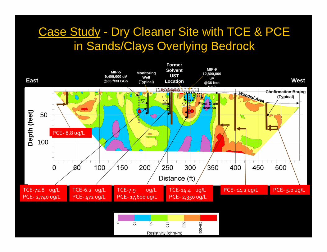
East West

Dep

th (

feet

)

Monitoring Well

(Typical)

Wooded Area

Confirmation Boring(Typical)

MIP-912,800,000

uV@36 feet

BGS

Floor DrainLocation

MIP-59,400,000 uV

@36 feet BGS

Former Solvent

USTLocation

PCE- 8.8 ug/L

TCE-72.8 ug/L

PCE- 2,740 ug/L

TCE-6.2 ug/L

PCE- 472 ug/L

TCE-7.9 ug/L

PCE- 17,600 ug/L

PCE- 14.2 ug/L PCE- 5.0 ug/LTCE-14.4 ug/L

PCE- 2,350 ug/L

Case Study - Dry Cleaner Site with TCE & PCEin Sands/Clays Overlying Bedrock

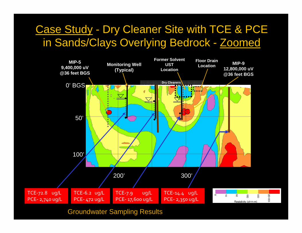
50

100

Dry Cleaners

Case Study - Dry Cleaner Site with TCE & PCEin Sands/Clays Overlying Bedrock - Zoomed

Monitoring Well(Typical)

MIP-912,800,000 uV@36 feet BGS

MIP-59,400,000 uV

@36 feet BGS

Former SolventUST

Location

100’

Dry Cleaners

50’

200’ 300’

0’ BGS

TCE-72.8 ug/L

PCE- 2,740 ug/L

TCE-6.2 ug/L

PCE- 472 ug/L

TCE-7.9 ug/L

PCE- 17,600 ug/L

TCE-14.4 ug/L

PCE- 2,350 ug/L

Groundwater Sampling Results

Floor DrainLocation

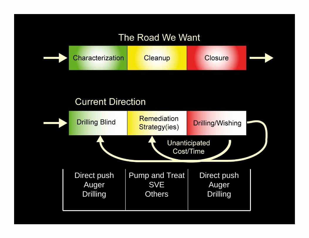
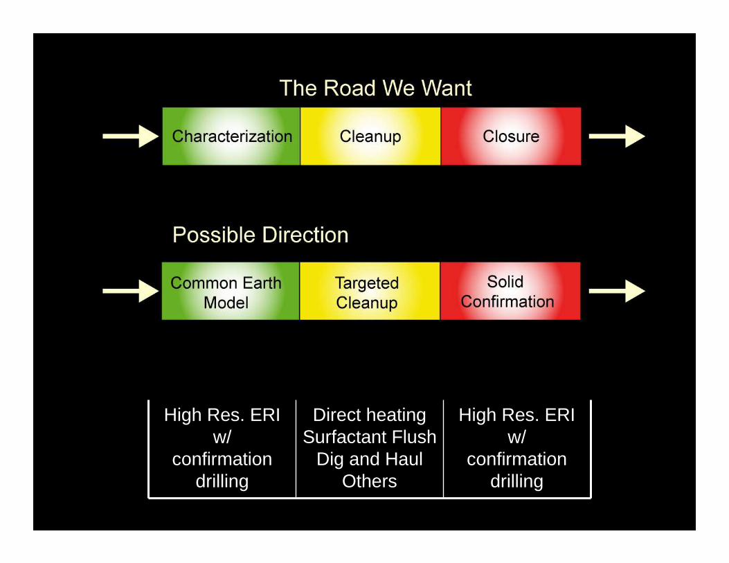
Direct pushAugerDrilling

Pump and TreatSVE

Direct pushAugerDrilling

Direct pushAugerDrilling

Pump and TreatSVE

Others

Direct pushAugerDrilling

High Res. ERIw/

confirmation drilling

Direct heatingSurfactant Flush

Dig and HaulOthers

High Res. ERIw/

confirmation drilling

Stop Drilling Blind!

Moral of This Story:

THANK YOU!THANK YOU!Questions?Questions?

Dr. Todd HalihanOklahoma State UniversitySchool of Geology105 Noble Research CenterStillwater, OK 74078todd.halihan@okstate.edu

Stuart W. McDonald, P.E.Aestus, LLC2605 Dotsero CourtLoveland, CO 80538(970) 278-4090swm@aestusllc.com

Reed T. TerryAestus, LLC4177 Route 2(518) 326-1279Troy, NY 12180rtt@aestusllc.com