General rights Copyright and moral rights for the publications made accessible in the public portal are retained by the authors and/or other copyright owners and it is a condition of accessing publications that users recognise and abide by the legal requirements associated with these rights. • Users may download and print one copy of any publication from the public portal for the purpose of private study or research. • You may not further distribute the material or use it for any profit-making activity or commercial gain • You may freely distribute the URL identifying the publication in the public portal If you believe that this document breaches copyright please contact us providing details, and we will remove access to the work immediately and investigate your claim. Downloaded from orbit.dtu.dk on: Jun 15, 2018 Drillstring Washout Diagnosis Using Friction Estimation and Statistical Change Detection Willersrud, Anders; Blanke, Mogens; Imsland, Lars; Pavlov, Alexey K. Published in: IEEE Transactions on Control Systems Technology Link to article, DOI: 10.1109/TCST.2015.2394243 Publication date: 2015 Document Version Peer reviewed version Link back to DTU Orbit Citation (APA): Willersrud, A., Blanke, M., Imsland, L., & Pavlov, A. K. (2015). Drillstring Washout Diagnosis Using Friction Estimation and Statistical Change Detection. IEEE Transactions on Control Systems Technology, 23(5), 1886- 1900. [7039260]. DOI: 10.1109/TCST.2015.2394243
Transcript
General rights Copyright and moral rights for the publications made accessible in the public portal are retained by the authors and/or other copyright owners and it is a condition of accessing publications that users recognise and abide by the legal requirements associated with these rights.
• Users may download and print one copy of any publication from the public portal for the purpose of private study or research. • You may not further distribute the material or use it for any profit-making activity or commercial gain • You may freely distribute the URL identifying the publication in the public portal
If you believe that this document breaches copyright please contact us providing details, and we will remove access to the work immediately and investigate your claim.
Downloaded from orbit.dtu.dk on: Jun 15, 2018
Drillstring Washout Diagnosis Using Friction Estimation and Statistical ChangeDetection
Willersrud, Anders; Blanke, Mogens; Imsland, Lars; Pavlov, Alexey K.
Published in:IEEE Transactions on Control Systems Technology
Link to article, DOI:10.1109/TCST.2015.2394243
Publication date:2015
Document VersionPeer reviewed version
Link back to DTU Orbit
Citation (APA):Willersrud, A., Blanke, M., Imsland, L., & Pavlov, A. K. (2015). Drillstring Washout Diagnosis Using FrictionEstimation and Statistical Change Detection. IEEE Transactions on Control Systems Technology, 23(5), 1886-1900. [7039260]. DOI: 10.1109/TCST.2015.2394243
Drillstring Washout Diagnosis using FrictionEstimation and Statistical Change Detection
Anders Willersrud, Mogens Blanke, SM IEEE,, Lars Imsland, Alexey Pavlov
Abstract—In oil and gas drilling, corrosion or tensile stress cangive small holes in the drillstring, which can cause leakage andprevent sufficient flow of drilling fluid. If such washout remainsundetected and develops, the consequence can be a completetwist-off of the drillstring. Aiming at early washout diagnosis,this paper employs an adaptive observer to estimate frictionparameters in the nonlinear process. Non-Gaussian noise is anuisance in the parameter estimates, and dedicated generalizedlikelihood tests are developed to make efficient washout detectionwith the multivariate t-distribution encountered in data. Changedetection methods are developed using logged sensor data from ahorizontal 1400 m managed pressure drilling test rig. Detectionscheme design is conducted using probabilities for false alarmand detection to determine thresholds in hypothesis tests. Amultivariate approach is demonstrated to have superior diag-nostic properties and is able to diagnose a washout at very lowlevels. The paper demonstrates the feasibility of fault diagnosistechnology in oil and gas drilling.
Index Terms—Managed pressure drilling, fault diagnosis,statistical change detection, adaptive observer, multivariate t-distribution, generalized likelihood ratio test
I. INTRODUCTION
Drilling is a major part of the total oil or gas field develop-ment cost. As the easy available reservoirs are being depleted,there is a trend that boundaries for drilling is pushed in thesense of more extreme environments, such as the arctic, ordeep wells with high pressure and high temperature. Withincreasing depth and drilling at more remote locations, the costof drilling is further increased and it is essential to minimizenon-productive time, that amounts to 20-25 % of total time inoperation [1].
Different incidents can happen downhole or topside thatcause downtime, or even abandonment of a well. Emergingadvanced drilling methods such as managed pressure drilling(MPD) [1], [2] brings along new instrumentation to the rig,which allows one to have methods for detecting abnormalsituations. One such situation is drillstring washout, which
Manuscript submitted February 28, 2014 to IEEE Transactions on ControlSystems Technology.
This work was supported by Statoil ASA and the Norwegian ResearchCouncil (NFR project 210432/E30 Intelligent Drilling).
A. Willersrud (corresponding author) and L. Imsland are with the De-partment of Engineering Cybernetics, Norwegian University of Scienceand Technology, N-7491 Trondheim, Norway, anders.willersrud,[email protected].
M. Blanke is with the Automation and Control Group, Department of Elec-trical Engineering, Technical University of Denmark, DK-2800 Kgs. Lyngby,Denmark and is affiliated with the AMOS Centre of Excellence, Department ofEngineering Cybernetics at NTNU in Trondheim, [email protected].
A. Pavlov is with the Department of Advanced Wells and En-hanced Oil Recovery, Statoil Research, N-3905 Porsgrunn, Norway,[email protected].
will be studied in this paper. A drillstring washout is a holeor cracks in the drillstring caused by wear, such as corrosionor tensile stress [3]. Such weakness can result in a completetwist-off of the pipe, which may cause an extra three to twelvedays of drilling, in worst case abandonment of the well [4].Early yet sure diagnosis of a drillstring washout is essential.The challenge is that a small washout gives tiny changes inpressure and flow rate of the circulated drilling fluid, and isdifficult to detect in noisy measurements signals. In additionto detecting the occurrence of the washout it is of great valueto isolate the position of the defect, making inspection andreplacement more effective.
Detection of other critical incidents have been studied usingdifferent detection methods. Probably the most studied case isan influx of formation fluid, or kick, see [5], [6], [7], [8]. Othersare lost circulation of drilling fluid to the formation, pack-offof drilling cuttings around the drillstring, and plugging of thedrill bit nozzles. All of these will affect drilling operation. Sim-ulation and detection of different downhole drilling incidents,including drillstring washout, were discussed in [9] with sometests on real data in [7]. There a high fidelity model was fittedto data and used to detect abnormalities. Knowledge-modelingwas used for classification of different incidents by [10] anda Bayesian network was shown to detect sensor and processfaults in [11].
A challenge with monitoring and diagnosis of downholeconditions in drilling is the lack of measurements. Mostcommonly, low frequency measurements with mud pulsetelemetry from the downhole assembly has been available [1].With high data rate, low latency transmission from downholesensors, actions can be taken at an earlier stage in order toavoid borehole stability problems [12]. Recently, wired drillpipe technology has emerged as a technology with distributedsensors along the drillstring, providing measurements at highsample rate in real time [1], [13].
Although increased instrumentation facilitates increased di-agnosis, there are still problems with measurement noise.Different statistical methods can be applied in order to increasedetection. In [5], a statistical cumulative sum (CUSUM) algo-rithm was applied in order to increase kick detection whilemaintaining a low false alarm rate. In [14], skewness of thestatistical distribution was used to detect poor hole cleaning.An adaptive observer for friction estimation was presented in[15] and applied on data in [16], but direct washout diagnosiswas not feasible due to very poor signal to noise propertieson the parameter estimates.
This paper proposes to use statistical change detectionmethods to diagnose downhole drilling incidents. The focus
2
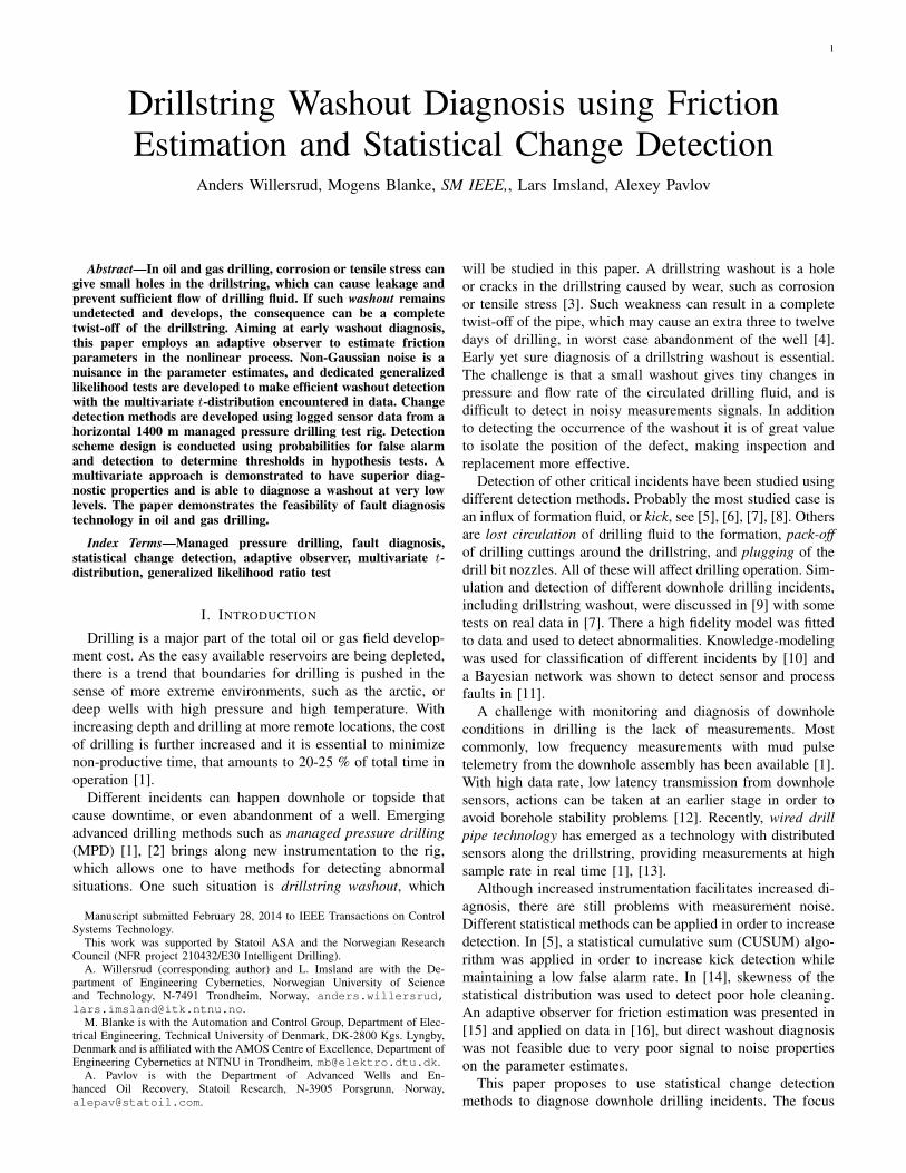
Figure 1. Overview of fault diagnosis method using an adaptive observer andstatistical change detection for fault diagnosis, where y are measurements, θare estimated parameters, and ∆µ(θ) is the change in mean of the estimatedparameters.
is on drillstring washout. The proposed method, depicted inFig. 1, consists of using a reasonably simple mathematicalmodel together with a nonlinear adaptive observer to estimatea set of friction parameters and combine this with dedicatedchange detection. The estimated parameters will remain (closeto) constant during normal operation, but change when thereis a washout in the system. Data from a medium scale flowloop designed and tested by the oil and gas company StatoilASA is used to test the diagnosis method. Due to noise in themeasurements the friction estimates are shown to be noticeablyaffected. Detection and isolation possibilities are studied usingthe changes that develop in estimated parameters during awashout. Dedicated change detection algorithms are derivedfor the multivariate t-distribution that is observed from data,based on a generalized likelihood ratio test (GLRT) approach.A GLRT for each parameter is tested against a threshold usingunivariate probability distributions of the noise, and changesto all parameters jointly can be considered using multivariatedistributions. Detectors are derived for both univariate andmultivariate distributions and their performances are com-pared.
Referring to Fig. 1, the scope of the paper is as follows.Sec. II presents the test rig and test scenarios, Sec. III presentsthe nonlinear dynamic model of the process, and the nonlinearadaptive observer used for parameter estimation (first blockin the figure). Sec. IV motivates the need for statisticalchange detection, and Sec. V presents an analysis of the noisedistribution of the estimated parameters. A dedicated diagnosisscheme is derived in Sec. VI for the multivariate t-distributionat hand (second block), and isolation of the washout position isanalyzed in Sec. VII (third block). Findings are validated usingexperimental data in Sec. VIII. A discussion and conclusioncompletes the paper.
II. FLOW-LOOP TEST FACILITY
To test the diagnosis methodology, we will use data fromtests on managed pressure drilling technology conducted byStatoil in a 1400 m horizontal flow loop test setup at premisesof the International Research Institute of Stavanger (IRIS),Norway. The flow loop was rigged with the possibility ofemulating various faults including drillstring washout.
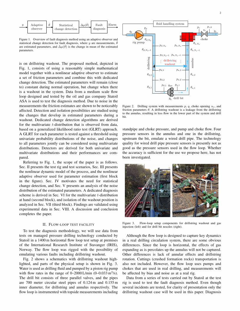
Fig. 2 shows a schematics with drillstring washout high-lighted, and parts of the physical setup is shown in Fig. 3.Water is used as drilling fluid and pumped by a piston rig pumpwith flow rates in the range of 0–2000 L/min (0–0.033 m3/s).The drill bit consists of three parallel valves, and the pipesare 700 meter circular steel pipes of 0.124 m and 0.155 minner diameter, for drillstring and annulus respectively. Theflow loop is instrumented with topside measurements including
Figure 2. Drilling system with measurements p, q, choke opening uc, andfriction parameters θ. A drillstring washout is a leakage from the drillstringto the annulus, resulting in less flow in the lower part of the system and drillbit.
standpipe and choke pressure, and pump and choke flow. Fourpressure sensors in the annulus and one in the drillstring,upstream the bit, emulate a wired drill pipe. The technologyquality for wired drill pipe pressure sensors is presently not asgood as the pressure sensors used in the flow loop. Whetherthe accuracy is sufficient for the use we propose here, has notbeen investigated.
Figure 3. Flow-loop setup components for drillstring washout and gasinjection (left) and for drill bit nozzles (right).
Although the flow loop is designed to capture key dynamicsin a real drilling circulation system, there are some obviousdifferences. Since the loop is horizontal, the effects of gasexpanding as is percolates up the annulus will not be captured.Other differences is lack of annular effects and drillstringrotation. Cuttings (crushed formation rocks) transportation isalso not included. However, the flow loop uses pumps andchokes that are used in real drilling, and measurements willbe affected by bias and noise as at a real rig.
Data from a series of tests carried out by Statoil at the testrig is used to test the fault diagnosis method. Even thoughseveral incidents are tested, for clarity of presentation only thedrillstring washout case will be used in this paper. Diagnosis
3
of other incidents is the topic in [17]. Drillstring washout is achallenging case with small changes to pressure due to friction,without any net change of flow in and out of the well. Toemulate drillstring washout, a valve located half way alongthe flow loop was gradually open, releasing the flow from thedrillstring section of the flow loop to the annulus section.
Table IFLOW-LOOP PHYSICAL PARAMETERS.
βd,a 2.2× 10⁹ Pa Effective bulk modulusρd,a 1000 kg/m3 Drilling fluid densityMa 3.74× 10⁷ Pa s2/m3 Integrated density per cross sectionMd 5.81× 10⁷ Pa s2/m3 Integrated density per cross sectionVa 13.2 m3 Volume of fluid in annulusVd 8.56 m3 Volume of fluid in drillstringhTVD 2.14 m True vertical depth of bitLd, La 700 m Length of drillstring/annulus
III. SYSTEM MODEL AND ADAPTIVE OBSERVER
The model-based fault diagnosis method in this paper isbased on parameter estimation using the simplified hydraulicsmodel in [18] as a process model together with an adaptiveobserver. As the authors argue, the simple model manages tocapture the key components of the flow dynamics in drilling.Furthermore, a high-fidelity model with many parameters maynot give a better result in practice, due to challenges inconfiguration and calibration. However, the simple model hassome limitations. In realistic situations, the particular bottomhole assembly (tools at the end of the drillstring) used may giveother setups near the bottom which may imply that detectedchanges in friction can be caused by other incidents thanthose considered herein. Moreover, we assume that the frictionpressure loss is in steady state, which means that care mustbe taken in interpreting detections in periods just after knowntransients such as changing pump rates, drilling bit off bottom,and change of drillstring rotational velocity.
The simple model has been applied for estimation andcontrol purposes in [8], [19], [20], [21]. This section presentsthe model as well as the adaptive observer utilizing wireddrill pipe measurements. The adaptive observer was derivedin [15], and used in a preliminary study on fault diagnosisof the flow loop data in [16], with simpler assumptions aboutthe noise probability distribution, detecting changes to eachfriction parameter separately.
A. Simplified hydraulic model
Referring to Fig. 2, let pp be the pressure at the pump, pc bethe pressure upstream the choke, and qbit the flow through thebit. The pump flow is denoted by qp, and qc is flow throughthe choke. The model used is based on the model in [18],given by
dppdt
=βdVd
(qp − qbit), (1a)
dpcdt
=βaVa
(qbit − qc(pc, u)) , (1b)
dqbit
dt=
1
M(pp−pc−F (θ, qbit)−(ρa−ρd)ghTVD) , (1c)
where ρj is the density, Vj the volume, and βj the bulk mod-ulus of the control volume indexed j ∈ {d, a} for drillstringand annulus, respectively. The true vertical depth of the wellis hTVD, g is the acceleration of gravity, and the integratedfluid density per cross section is M =
∫ L0
ρ(x)A(x)dx where L is
the total length from pump to choke, and A(x) is the crosssection at position x. The unknown friction parameter vectorθ is estimated by the adaptive observer. The total friction ismodeled by
F (θ, q) = θbfb(q) +
Nd∑i=1
θd,ifd(q) +
Na∑i=1
θa,ifa(q), (2)
where fd(q), fb(q), and fd(q) model the flow characteristicsin the drillstring, bit, and annulus, respectively, and θ is avector of assumed constant friction parameters to be estimated.The friction is more accurately modeled by complex modelsdepending on well geometry and the non-Newtonian propertiesof drilling fluids, but in the spirit of simple models to beupdated by measurements, we will here assume that f(q)is given by f(q) = q for laminar flow and f(q) = q2 forturbulent flow. The flow through the choke is given by
qc(pc, u) = sgn(pc − pc,0)gc(uc)√|pc − pc,0|, (3)
where gc(uc) is the choke characteristics found empirically forchoke opening uc ∈ [0, 100], pc,0 is the pressure downstreamthe choke.
Wired drill pipe technology extends the number of pressuremeasurements downhole. Let pd,i, i ∈ {1, . . . , Nd} be themeasurements in the drillstring, and pa,i, i ∈ {1, . . . , Na} inthe annulus, see Fig. 2. The pressure difference is a functionof friction and hydrostatic pressure,
where Gj,i = ρjg(hj,i − hj,i+1) is the hydrostatic pressuredifference between sensor pj,i at depth hj,i and sensor pj,i+1 atdepth hj,i+1. The corresponding friction between the sensors isgiven by θj,ifj(q), where θj,i is the constant friction parameterand fj(q) is the flow characteristics in the drillstring andannulus, respectively. For typical flow rates in the test rig theReynolds number is large enough to indicate turbulent flowin both drillstring and annulus, giving fd(q) = fa(q) = q2,which also was found empirically in [17]. The pressure dropover the drill bit is given by
pa,1 = pd,1 − θbfb(q), (5)
where θb is the friction parameter in the drill bit. The flowcharacteristics fb(q) is typically given by fb(q) = q2, see,e.g., [22].
B. Nonlinear adaptive observer
Estimation of parameters in the nonlinear system could beachieved by extensions to the extended Kalman filtering (EKF)techniques that estimate noise covariance online and hencewould not need knowledge of noise and process disturbancecovariances. This is described for linear systems in [23],
4
and [24] extended the EKF to continuous nonlinear systemswith discrete time measurements. Also the later particle fil-ter approaches could be applied. Here, a nonlinear observerapproach is used that is based on deterministic stability anal-ysis but still relies on persistent excitation to get parameterconvergence.
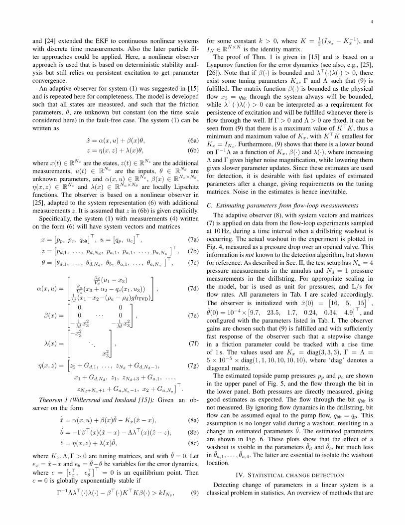
An adaptive observer for system (1) was suggested in [15]and is repeated here for completeness. The model is developedsuch that all states are measured, and such that the frictionparameters, θ, are unknown but constant (on the time scaleconsidered here) in the fault-free case. The system (1) can bewritten as
where x(t) ∈ RNx are the states, z(t) ∈ RNz are the additionalmeasurements, u(t) ∈ RNu are the inputs, θ ∈ RNθ areunknown parameters, and α(x, u) ∈ RNx , β(x) ∈ RNx×Nθ ,η(x, z) ∈ RNz and λ(x) ∈ RNu×Nθ are locally Lipschitzfunctions. The observer is based on a nonlinear observer in[25], adapted to the system representation (6) with additionalmeasurements z. It is assumed that z in (6b) is given explicitly.
Specifically, the system (1) with measurements (4) writtenon the form (6) will have system vectors and matrices
where Kx,Λ,Γ > 0 are tuning matrices, and with θ = 0. Letex = x−x and eθ = θ−θ be variables for the error dynamics,where e =
[e>x , e>θ
]>= 0 is an equilibrium point. Then
e = 0 is globally exponentially stable if
Γ−1Λλ>(·)λ(·)− β>(·)K>Kβ(·) > kINθ , (9)
for some constant k > 0, where K = 12 (INx − K−1
x ), andIN ∈ RN×N is the identity matrix.
The proof of Thm. 1 is given in [15] and is based on aLyapunov function for the error dynamics (see also, e.g., [25],[26]). Note that if β(·) is bounded and λ>(·)λ(·) > 0, thereexist some tuning parameters Kx, Γ and Λ such that (9) isfulfilled. The matrix function β(·) is bounded as the physicalflow x3 = qbit through the system always will be bounded,while λ>(·)λ(·) > 0 can be interpreted as a requirement forpersistence of excitation and will be fulfilled whenever there isflow through the well. If Γ > 0 and Λ > 0 are fixed, it can beseen from (9) that there is a maximum value of K>K, thus aminimum and maximum value of Kx, with K>K smallest forKx = INx . Furthermore, (9) shows that there is a lower boundon Γ−1Λ as a function of Kx, β(·) and λ(·), where increasingΛ and Γ gives higher noise magnification, while lowering themgives slower parameter updates. Since these estimates are usedfor detection, it is desirable with fast updates of estimatedparameters after a change, giving requirements on the tuningmatrices. Noise in the estimates is hence inevitable.
C. Estimating parameters from flow-loop measurementsThe adaptive observer (8), with system vectors and matrices
(7) is applied on data from the flow-loop experiments sampledat 10 Hz, during a time interval when a drillstring washout isoccurring. The actual washout in the experiment is plotted inFig. 4, measured as a pressure drop over an opened valve. Thisinformation is not known to the detection algorithm, but shownfor reference. As described in Sec. II, the test setup has Na = 4pressure measurements in the annulus and Nd = 1 pressuremeasurements in the drillstring. For appropriate scaling inthe model, bar is used as unit for pressures, and L/s forflow rates. All parameters in Tab. I are scaled accordingly.The observer is initialized with x(0) =
[16, 5, 15
]>,
θ(0) = 10−4×[9.7, 23.5, 1.7, 0.24, 0.34, 4.9
]>, and
configured with the parameters listed in Tab. I. The observergains are chosen such that (9) is fulfilled and with sufficientlyfast response of the observer such that a stepwise changein a friction parameter could be tracked with a rise timeof 1 s. The values used are Kx = diag(3, 3, 3), Γ = Λ =5 × 10⁻⁵ × diag(1, 1, 10, 10, 10, 10), where ‘diag’ denotes adiagonal matrix.
The estimated topside pump pressures pp and pc are shownin the upper panel of Fig. 5, and the flow through the bit inthe lower panel. Both pressures are directly measured, givinggood estimates as expected. The flow through the bit qbit isnot measured. By ignoring flow dynamics in the drillstring, bitflow can be assumed equal to the pump flow, qbit = qp. Thisassumption is no longer valid during a washout, resulting in achange in estimated parameters θ. The estimated parametersare shown in Fig. 6. These plots show that the effect of awashout is visible in the parameters θd and θb, but much lessin θa,1, . . . , θa,4. The latter are essential to isolate the washoutlocation.
IV. STATISTICAL CHANGE DETECTION
Detecting change of parameters in a linear system is aclassical problem in statistics. An overview of methods that are
5
Figure 4. Actual washout in experiment measured over washout emulationvalve, measured as pressure loss at different flow rates {q0, . . . , q6}. Thecolor coding shown to the right shows the pressure drop ∆p(qi) for each flowrate qi, where higher flow rates give higher pressure drop. This informationis not known to the diagnosis methods, but shown for reference.
Figure 5. State estimation and measurements of pump pressure (pp), chokepressure (pc), and bit flow/pump flow (qbit/qp) during a washout. The flowrate and choke pressure is constant, while the pump pressure decreases duringthe washout due to reduced friction in the system.
Figure 6. Estimated parameters θd, θb and θa1 to θa4.
applicable for linear systems with Gaussian noise is providedin [27]. When the quantities for which change detectionare desired have non-Gaussian distributed noise, the changedetection problem is harder but solvable. When the quantitiesunder test are time-wise correlated and non-Gaussian, testscan be achieved but analytical methods may not be availableto determine thresholds that give desired false alarm anddetection probabilities.
A widely applied methodology is based on a likelihood ratiotest, which maximizes the probability of detection PD with agiven false alarm probability PFA [28]. The test will differ-entiate between the null hypothesis H0 and the alternativehypothesis H1 using the probability density function (PDF)under each hypothesis. If the statistical parameters under H1
are unknown, the generalized likelihood ratio test (GLRT) canbe applied.
The proposed method in this paper is to use parameterestimation to track physical changes in friction. With noise inthe measurement, and with desired fast detection, parameterestimates are inevitably subjected to random variation. Thusis statistical change detection used to obtain desired falsealarm rate and detection properties. Statistical change detectionfurthermore gives us isolation capability with known statisticalproperties. Methods for statistical change detection in faultdiagnosis were applied in [29], [30] and applications arereferred in [31] where GLRT was employed for detectingchange in estimated parameters.
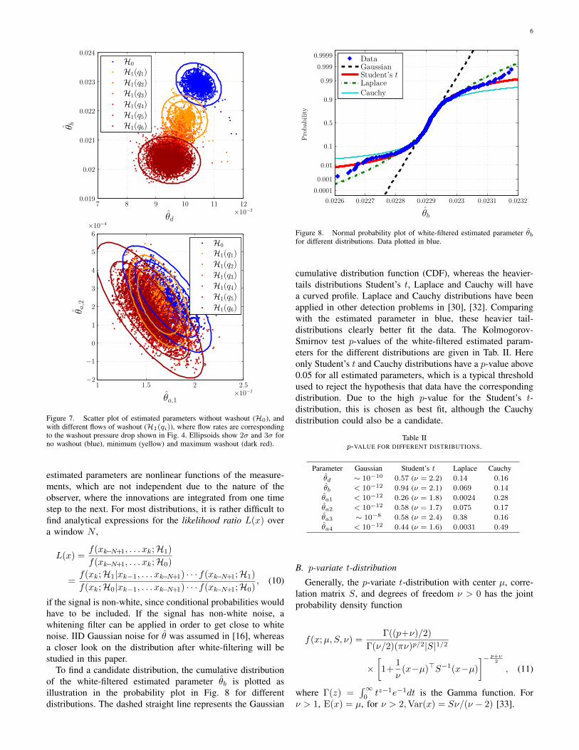
The need for statistical change detection is illustrated byinspecting θd and θb plotted in Fig. 6, which are affectedthe most by a drillstring washout. Fig. 7 shows the fault freecase H0, and the fault-case H1(qi) for different washout flowrates qi, see Fig. 4. The contour lines show two and threestandard deviations calculated as if data were Gaussian. Theupper plot illustrates that the small washout flow rate q1 isdifficult to detect from the parameters while keeping the falsealarm rate low. For the friction parameters θa,1 and θa,2 inthe annulus in the lower plot in Fig. 7, it is not possible todistinguish the different cases. Without a statistical changedetection approach, it may be possible to detect a washoutthrough change in θd and θb, albeit with poor false alarmversus detection performance, but it would not be possible todetermine the washout position.
V. PROBABILITY DISTRIBUTION
The statistical change detection algorithm presented inSec. VI utilizes the probability density function (PDF) ofthe noise in order to detect a change. With a vector ofestimated parameters θ, it is possible to detect a change in eachparameter isolated, using univariate distributions, or to jointlydetect change in the multivariate distribution. The differentdistributions will be presented in this section.
A. Probability distribution of estimated parameters
Most commonly the noise of a signal is assumed to be in-dependent, identically distributed (IID) Gaussian white noise.However, if the noise of the signal has heavier tails it willbe more accurately represented with another distribution. The
6
Figure 7. Scatter plot of estimated parameters without washout (H0), andwith different flows of washout (H1(qi)), where flow rates are correspondingto the washout pressure drop shown in Fig. 4. Ellipsoids show 2σ and 3σ forno washout (blue), minimum (yellow) and maximum washout (dark red).
estimated parameters are nonlinear functions of the measure-ments, which are not independent due to the nature of theobserver, where the innovations are integrated from one timestep to the next. For most distributions, it is rather difficult tofind analytical expressions for the likelihood ratio L(x) overa window N ,
if the signal is non-white, since conditional probabilities wouldhave to be included. If the signal has non-white noise, awhitening filter can be applied in order to get close to whitenoise. IID Gaussian noise for θ was assumed in [16], whereasa closer look on the distribution after white-filtering will bestudied in this paper.
To find a candidate distribution, the cumulative distributionof the white-filtered estimated parameter θb is plotted asillustration in the probability plot in Fig. 8 for differentdistributions. The dashed straight line represents the Gaussian
Figure 8. Normal probability plot of white-filtered estimated parameter θbfor different distributions. Data plotted in blue.
cumulative distribution function (CDF), whereas the heavier-tails distributions Student’s t, Laplace and Cauchy will havea curved profile. Laplace and Cauchy distributions have beenapplied in other detection problems in [30], [32]. Comparingwith the estimated parameter in blue, these heavier tail-distributions clearly better fit the data. The Kolmogorov-Smirnov test p-values of the white-filtered estimated param-eters for the different distributions are given in Tab. II. Hereonly Student’s t and Cauchy distributions have a p-value above0.05 for all estimated parameters, which is a typical thresholdused to reject the hypothesis that data have the correspondingdistribution. Due to the high p-value for the Student’s t-distribution, this is chosen as best fit, although the Cauchydistribution could also be a candidate.
If each parameter is considered individually, a univariate t-distribution with p = 1 can be used to represent the distributionof the estimated parameters. If changes to all parameters areconsidered simultaneously, the p = Nθ multivariate distribu-tion will have to be used.
The degrees of freedom ν in the univariate Student’s t-distribution are also listed in Tab. II for each estimatedparameter. Note that the if ν = 1, (11) is the p-variateCauchy distribution. If ν →∞, (11) is the p-variate Gaussiandistribution [33].
VI. GENERALIZED LIKELIHOOD RATIO TEST
The size of the washout affects the magnitude of changein the friction parameters, but the magnitude of change isunknown. A generalized likelihood ratio test (GLRT) canhence be applied for change detection. The GLRT utilizesthe distribution of the noise in the estimated parametersto best fit a t-distribution. In this section, the GLRT forunivariate distributions is described, together with multivariatedistributions where the direction of change is assumed knownor unknown, respectively.
Change detection for parameters with Gaussian noise werethoroughly treated in [27], a GLRT detector was derived forCauchy distributed test quantities in [34], but a GLRT detectorfor the t-distribution has not been found in the literature.
A. GLRT with univariate Student’s t-distribution
To detect changes in the vector of estimated friction pa-rameters, changes to each parameter can be considered in-dependently, using a generalized likelihood ratio test withunivariate Student’s t-distributions. The detection problemis to differentiate whether a signal x belongs to the nullhypothesis H0 or the alternative hypothesis H1. If only thestatistical parameter µ changes, whereas σ and ν are assumedconstant, the detection problem with θ ∈ R is
H0 : θ ∼ t(µ0, σ, ν), (12a)
H1 : θ ∼ t(µ1, σ, ν). (12b)
To reduce computational cost, the window-limited GLRT isused where 0 ≤ N < N [35], [36], which is given by
g(k) = maxk−N+1≤j≤k−N
ln
∏ki=j f(θ(i); µ1, σ, ν)∏ki=j f(θ(i);µ0, σ, ν)
, (13)
where µ1 is the maximum likelihood estimate of the mean µ1
at H1, and f(x;µ, σ, ν) is the univariate PDF (11) with p = 1.A change between the hypotheses (12) is detected if the
decision function g(k) is above a threshold h,
if g(k) ≤ h accept H0,
if g(k) > h accept H1.
With univariate distributions, Nθ decision functions g(k; θi)will have to be checked against corresponding thresholds hi.
B. GLRT with multivariate t-distribution and known directionof change
Detecting a change in a multivariate Gaussian distributionwhere the direction is known but magnitude unknown, isdescribed in [37], [38]. This is generalized to the multivariatet-distribution in this section, and the derivation is provided inAppendix B.
Let the change detection problem with θ ∈ RNθ be
H0 : θ ∼ t(µ0, S, ν),
H1 : θ ∼ t(µ0 + wΥ, S, ν),
where w is the change magnitude and Υ is the change directionwith ‖Υ‖ = 1, assuming that S and ν are unchanged. Thegeneralized likelihood ratio decision function [37], [28] isgiven by
g(k) = maxk−N+1≤j≤k−N
lnsupw
∏ki=j f(θ(i);µ0+wΥ, S, ν)∏ki=j f(θ(i);µ0, S, ν)
.
(14)
With a derivation (see Appendix B) similar to that of amultivariate normal distribution in [37], [38], the estimate ofmagnitude of change with distribution (11) is
w(k, j) =Υ>S−1(Θ(k, j)− µ0)
Υ>S−1Υ, (15)
where
Θ(k, j) =1
k−j+1
k∑i=j
θ(i). (16)
The resulting decision function will then be
g(k) = maxk−N+1≤j≤k−N
p+ν
2
k∑i=j[
− ln
(1 +
1
ν(θ(i)−µ0−wΥ)>S−1(θ(i)−µ0−wΥ)
)+ ln
(1 +
1
ν(θ(i)−µ0)>S−1(θ(i)−µ0
))
]. (17)
C. GLRT with multivariate t-distribution and unknown direc-tion of change
If no assumption of direction of change is assumed, theMLE µ1 of the mean at H1 has to be found. From AppendixA, the MLE of the mean µ1 is given by
µ1 =1
k−j+1
k∑i=j
θ(i), (18)
and the GLR decision function is given by
g(k) = maxk−N+1≤j≤k−N
p+ν
2
k∑i=j[
− ln
(1 +
1
ν(θ(i)−µ1)>S−1(θ(i)−µ1)
)+ ln
(1 +
1
ν(θ(i)−µ0)>S−1(θ(i)−µ0)
)]. (19)
8
D. Thresholds based on GLRT test statistic approximated bya Weibull distribution
If the GLRT input was Gaussian and IID, the test statisticg(k) would asymptotically follow a χ2
r distribution and withr unknown parameters, r degrees of freedom under H0, and anon-central χ′2r (λ) distribution with non-centrality parameter λunder H1 [28]. This would make it possible to set a thresholdcorresponding to a desired probability of false alarms andof detection. However, for real applications with correlatedinput, g(k) is not χ2
r distributed. Distributions seen in realapplications depend on properties of the case. A Weibulldistribution best fitted residuals from aircraft attitude data in[30]; a lognormal distribution best fitted the GLRT test statisticfrom narrow band correlated ship motion data in [29]. Thedistribution of the test statistic is therefore studied in thissection, based on real data.
Having tested several possibilities, the Weibull distributionwas found to give a good fit to the test statistic. The Weibulldistribution has the probability distribution F (x;α, β) and thedensity function f(x;α, β), given by
F (x;α, β) = 1− e−(x/α)β , x ≥ 0, (20a)
f(x;α, β) =β
α
(xα
)β−1
e−(x/α)β , x ≥ 0, (20b)
where α > 0 is the scale parameter and β > 0 the shapeparameter.
Let PFA be the probability of false alarm under H0. Thenusing the inverse CDF gives a threshold h with the givenprobability PFA,
The given threshold h will also determine the probabilityof detecting a fault under hypothesis H1 with probability PD,
PD = 1− F (h;H1, α1, β1) = e−(h/α1)β1 . (22)
VII. FAULT DIAGNOSIS
Changes to the different parameters are used to detect awashout and isolate its position. As seen in Fig. 2, a washoutwill decrease the flow in the lower parts of the drillstring andthe annulus, as well as in the drill bit. This will result ina decrease in the estimated parameters, since the estimatorassumes equal flow throughout the system. Friction changesin the drillstring and bit are considerably higher than in theannulus, and they are thus used for detection. A washout isdetected if both θd and θb have a negative change, as listedin Tab. III. At the position of the washout, the related frictionparameter will have a positive change. There will still be somefriction loss in this section, however only the pressure sensorin the beginning of the section will be affected by reducedflow. The net effect is an increase in pressure drop in thissection, which is used to isolate the washout. The other annularfriction parameters must be unchanged or changing in negativedirection.
Table IIIFAULT ISOLATION OF DRILLSTRING WASHOUT WITH INCREASING (+),
DECREASING (−) AND UNCHANGED (0) VARIABLES. X DENOTESIGNORED CHANGE IN PARAMETER.
A. Isolation based on individual parameter changes withunivariate distributions
If changes to each parameter are individually considered, aGLRT on each estimated parameter is used for fault diagnosis.There will be one threshold for each estimated parameter,determined based on a specified probability PFA of false alarm.Let the possible faults be
fi ∈ F , (23)
where fi represents a washout between sensor pa,i and pa,i+1,corresponding to friction parameter θa,i, and F are all possiblelocations of washout. Location of washout position fromfriction parameters are listed in Tab. III, based on the changesto friction shown in Fig. 2. If the changes in estimated annulusparameters are inconsistent with regards to rows in Tab. III,the position cannot be isolated, although a washout may stilldetected if θd and θb have a negative change (f0).
B. Isolation in multivariate distribution with known directionof change
If the direction of change is limited to the possible knownvectors of change directions Υi ∈ Y , isolation is done byfinding the Υi with the largest change magnitude w. Thiswill reduce the problem of inconsistent changes to parametersas found in the univariate case in Sec. VII-A, due to someparameters being below its threshold.
For each data sample, the largest w(Υi) is found from (15)with fault isolation position
fisol := arg maxi w(Υi) =Υ>i S
−1(Θ(k, j)− µ0)
Υ>i S−1Υi
, (24)
and used to find the value of g(k) in (17) with w(Υi|i = fisol).Hence is it only necessary to calculate g(k) for one type offault, although (15) will have to be calculated for each Υi.
C. Isolation in multivariate distribution with unknown direc-tion of change
In this case, the fault fisol ∈ F can be isolated by findingthe largest projection of change in mean (µ1 − µ0) onto thevectors Υi ∈ Y ,
fisol = arg maxiΥ>i (µ1 − µ0)
Υ>i Υi. (25)
The difference between this method and the known directioncase in Sec. VII-B is that µ1 is used explicitly in the decision
9
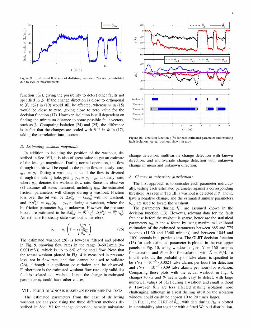
Figure 9. Estimated flow rate of drillstring washout. Can not be validateddue to lack of measurements.
function g(k), giving the possibility to detect other faults notspecified in Y . If the change direction is close to orthogonalto Y , g(k) in (19) would still be affected, whereas w in (15)would be close to zero, giving close to zero value for thedecision function (17). However, isolation is still dependent onfinding the minimum distance to some possible fault vectors,such as Y . Comparing isolation (24) and (25), the differenceis in fact that the changes are scaled with S−1 in w in (17),taking the correlation into account.
D. Estimating washout magnitude
In addition to isolating the position of the washout, de-scribed in Sec. VII, it is also of great value to get an estimateof the leakage magnitude. During normal operation, the flowthrough the bit will be equal to the pump flow at steady state,qbit = qp. During a washout, some of the flow is divertedthrough the leaking hole, giving qwo = qp−qbit at steady state,where qwo denotes the washout flow rate. Since the observer(8) assumes all states measured, including qbit, the estimatedfriction parameters will change during a washout. Frictionloss over the bit will be ∆pH0
bit = kbitq2p with no washout,
and ∆pH1
bit = kbit(qp − qwo)2 during a washout, where thebit friction parameter kbit is unknown. However, the pressurelosses are estimated to be ∆pH0
bit = θH0
b q2p, ∆pH1
bit = θH1
b q2p.
An estimate for steady state washout is therefore
qwo = qp
(1−
√θH1
b
θH0
b
). (26)
The estimated washout (26) is low-pass filtered and plottedin Fig. 9, showing flow rates in the range 0–60 L/min (0–0.001 m3/s), which is up to 6 % of the total flow. Note thatthe actual washout plotted in Fig. 4 is measured in pressureloss, not in flow rate, and thus cannot be used to validate(26), although a significant co-variation can be observed.Furthermore is the estimated washout flow rate only valid if afault is isolated as a washout. If not, the change in estimatedparameter θb could have other causes.
VIII. FAULT DIAGNOSIS BASED ON EXPERIMENTAL DATA
The estimated parameters from the case of drillstringwashout are analyzed using the three different methods de-scribed in Sec. VI for change detection, namely univariate
Figure 10. Decision function g(k) for each estimated parameter and resultingfault isolation. Actual washout shown in gray.
change detection, multivariate change detection with knowndirection, and multivariate change detection with unknownchange in mean and unknown direction.
A. Change in univariate distributions
The first approach is to consider each parameter individu-ally, testing each estimated parameter against a correspondingthreshold. As seen in Tab. III, a washout is detected if θd and θbhave a negative change, and the estimated annular parametersθa,i are used to locate the washout.
The parameters during H0 are assumed known in thedecision function (13). However, relevant data for the faultfree case before the washout is sparse, hence are the statisticalparameters µ0, σ and ν found by using maximum likelihoodestimation of the estimated parameters between 685 and 775seconds (11:30 and 13:00 minutes), and between 1045 and1100 seconds in a previous test. The GLRT decision function(13) for each estimated parameter is plotted in the two upperpanels in Fig. 10, using window lengths N = 150 samplesfor detection and N = 400 for isolation, with N = N/4. Tofind thresholds, the probability of false alarm is specified tobe PFA = 10−5 (0.0024 false alarms per hour) for detectionand PFA = 10−3 (0.09 false alarms per hour) for isolation.Comparing these plots with the actual washout in Fig. 4,changes to θd and θb seem quite easy to detect, with largenumerical values of g(k) during a washout and small withoutit. However, θa,i are less affected making isolation morechallenging, although in a real drilling situation the isolationwindow could easily be chosen 10 to 20 times larger.
In Fig 11, the GLRT of θa,3 with data during H0 is plottedin a probability plot together with a fitted Weibull distribution.
10
Figure 11. Weibull probability plot of GLRT underH0,H1(q1) andH1(q6)for estimated parameter θa,3 fitted to Weibull distributions. Threshold shownwith dashed line.
This friction parameter will determine isolation of the washout.Also plotted is data under hypothesis H1 with washout flowrate q1 corresponding to a pressure loss between 1 and 2bar, see Fig. 5, and flow rate q6 with pressure loss of 8 bar.The statistical parameters of the fitted Weibull distributions(20a) during H0, H1(q1) and H1(q6) are listed in Tab. IV,also showing the corresponding threshold values and detectionprobabilities PD. For convenience, the table shows the misseddetection probability PM = 1− PD.
As illustrated in Fig. 11, θa,3 has a quite small value forprobability of detection at q1, meaning that isolation for smallwashout flow rates is quite uncertain. If PD was to increase,the threshold should be lower with a penalty in increased PFA.
Using the thresholds listed in Tab. IV, the resulting faultisolation is shown in the bottom of Fig. 10. Isolation of theposition is quite uncertain in the first 3 minutes where thewashout is ramping up (q1 and q2). When the washout ratereaches a high level, isolation is quite certain. The reason forno isolation for a short period at around 13 and 15 minutesis due to a longer window for isolation than for detection,combined with a sudden change in washout flow rate. Theestimated θa,3 is above the threshold for the first two minutes,even though there are no faults. The reason is probably dueto external factors (disturbances) in the process.
B. Multivariate distribution with known direction of change
The second case is to use the multivariate distribution, andlimit the possible directions of change to a predefined set ofvectors Υi ∈ Y , as described in Sec.VI-B, with isolationas described in Sec. VII-B. The assumed possible changedirections for detection and isolation are column vectors of
Υdet =
[−1−3
], Υisol =
1 −1 −1 −10 1 −1 −10 0 1 −10 0 0 1
, (27)
Figure 12. Decision function g(k) with known direction of change Υ.Isolation based on largest w for each direction of change Υi ∈ Y , withg(k) plotted for each direction. Actual washout shown in gray.
where Υi = Υi/||Υi||. The magnitude of the friction pa-rameter in the bit increases approximately three times themagnitude of the friction parameter in the drillstring. It isassumed that all parameters in the annulus are affected equally.
The white-filtered estimated parameters θdet ∈ RNd+1 andθisol ∈ RNa are fitted to a multivariate t-distributions using theECME algorithm [39]. The decision functions for detectionand isolation are plotted in Fig. 12, together with resultingisolation. In the middle panel, the isolation functions gisol(k)are plotted for each Υi ∈ Y , showing that a washout atposition three gives the highest value. Note that isolationis based on maximum w(Υi) given by (24), and thus onlyone decision function is required to be calculated. Parametervalues, thresholds and detection probabilities are listed inTab. V. The threshold value h for gdet(k) was selected to givea false alarm probability PFA = 10−5 from the data underH0, for isolation PFA = 10−3 is used.
No washout is isolated in the first three minutes. The reasonmay be that changes in the parameters do not corresponddirectly to the directions (27). Furthermore may these di-rections not be entirely accurate, where also correlation Saffects the change direction (15). Compared to the univariatecase in Fig. 10, accuracy in isolated position is increased forhigher washout flow rates (after six minutes). The detectionprobability PD is higher for the multivariate method, and forhigher washout rates the detection probability in isolation issignificantly higher (lower PM ).
11
Table IVTHRESHOLD AND PROBABILITY OF DETECTION BASED ON FITTED WEIBULL DISTRIBUTIONS WITH PARAMETERS α AND β , WITH CHANGES TO
INDEPENDENT UNIVARIATE DISTRIBUTIONS.
PFA N h α0 β0 α1(q1) β1(q1) α1(q6) β1(q6) PM (q1) PM (q6)
C. Multivariate distribution with unknown change in meanand unknown direction
In the third case, no assumption about change directionis made in the decision function, making it sensitive to allchanges. Isolation given by (25) is done by finding the changein mean closest to possible change vectors, here given by (27).
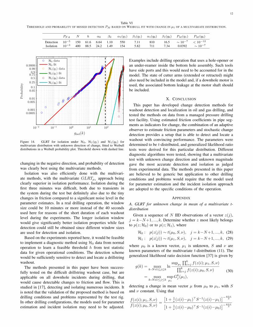
The decision function gdet(k) for the multivariate distri-bution of θd and θb is plotted in the top of Fig. 13, whichis used for detection. Parameters θa,i are used for isolation,with detection function gisol(k) plotted in the middle panel.Isolation is plotted in the lower panel. The thresholds arebased on fitted data to Weibull probability functions, plottedfor gisol(k) in Fig. 14. Comparing with the univariate method inFig. 11, much less of theH1 data is left of the threshold, givingbetter isolation. Parameter values, thresholds and detectionprobabilities are listed in Tab. VI.
With this method a washout is detected almost immediatelyand is isolated around the 3 minutes time stamp. The differ-ence between this very successful approach and the previousmethod is that assumption about direction is only made forisolation. Furthermore, isolation is only done based on changesin mean (25), not scaled with S as in (24).
IX. DISCUSSION
The friction model used in the adaptive observer is quitesimple, but proved to work satisfactory for the washout case.If the method was to be applied during a large range of pumpflow rates and with different drilling fluid densities, a moresophisticated friction model may be required. Nevertheless, forthe current process, it has been sufficient in order to provideconvincing detection of washout and isolation of the positionof the leakage.
Two vector-based (multivariate) methods were compared.Method one, GLRTwΥ, assumed a known direction Υ, butunknown magnitude w. The direction vectors were deter-mined from expected changes to the parameters with differentwashout locations. The second method, GLRTµ1
, assumed anunknown direction and magnitude of change in the vector µ1.
Figure 13. Decision function g(k) with unknown change in mean andunknown direction of change. Isolation based on finding change in meanclosest to possible change directions Υi ∈ Y . Actual washout shown in gray.
The main difference between the two multivariate methodswas that method one limits detection to already specifiedfault directions, other faults may not be detected. Methodtwo calculates g(k) based on the new estimated directionof change, and then isolates the position based on alreadyassumed known directions. A disturbance not correspondingto the defined directions would impact the decision functionin the second case, but much less in the first. A challenge canbe to find the correct change directions. In this study, therewas only data from one washout location available, the othersare assumed with same structure and values.
Detection was based on both drillstring and bit parameters
12
Table VITHRESHOLD AND PROBABILITY OF MISSED DETECTION PM BASED ON WEIBULL FIT WITH CHANGE IN µ1 OF A MULTIVARIATE DISTRIBUTION.
PFA N h α0 β0 α1(q1) β1(q1) α1(q6) β1(q6) PM (q1) PM (q6)
Figure 14. GLRT for isolation under H0, H1(q1) and H1(q6) formultivariate distribution with unknown direction of change, fitted to Weibulldistributions in a Weibull probability plot. Threshold shown with dashed line.
changing in the negative direction, and probability of detectionwas clearly best using the multivariate methods.
Isolation was also efficiently done with the multivari-ate methods, with the multivariate GLRTµ1 approach beingclearly superior in isolation performance. Isolation during thefirst three minutes was difficult, both due to transients inthe system during the test but definitely also due to the tinychanges in friction compared to a significant noise level in theparameter estimates. In a real drilling operation, the windowsize could be 10 minutes or more instead of the 40 secondsused here for reasons of the short duration of each washoutlevel during the experiments. The longer isolation windowwould give significantly better isolation properties while fastdetection could still be obtained since different window sizesare used for detection and isolation.
Based on the experiments reported here, it would be feasibleto implement a diagnostic method using H0 data from normaloperation to learn a feasible threshold h from test statisticdata for given operational conditions. The detection schemewould be sufficiently sensitive to detect and locate a drillstringwashout.
The methods presented in this paper have been success-fully tested on the difficult drillstring washout case, but areapplicable on all downhole incidents during drilling, thatwould cause detectable changes to friction and flow. This isstudied in [17], detecting and isolating numerous incidents. Itis noted that the validation of the proposed method is based ondrilling conditions and problems represented by the test rig.In other drilling configurations, the models used for parameterestimation and incident isolation may need to be adjusted.
Examples include drilling operation that uses a hole-opener oran under-reamer inside the bottom hole assembly. Such toolshave side ports and this would need to be accounted for in themodel. The state of cutter arms (extended or retracted) mightalso need be included in the model and, if a downhole motor isused, the associated bottom leakage at the motor shaft shouldbe included.
X. CONCLUSION
This paper has developed change detection methods forwashout detection and localization in oil and gas drilling, andtested the methods on data from a managed pressure drillingtest facility. Using estimated friction coefficients in pipe seg-ments as indicators for change, the combination of an adaptiveobserver to estimate friction parameters and stochastic changedetection provides a setup that is able to detect and locate awashout with convincing performance. The parameters weredetermined to be t-distributed, and generalized likelihood ratiotests were derived for this particular distribution. Differentdiagnostic algorithms were tested, showing that a multivariatetest with unknown change direction and unknown magnitudegave the most accurate detection and isolation as judgedfrom experimental data. The methods presented in this paperare believed to be generic but application to other drillingconditions and problems would require that the model usedfor parameter estimation and the incident isolation approachare adopted to the specific conditions of the operation.
APPENDIX
A. GLRT for unknown change in mean of a multivariate t-distribution
Given a sequence of N IID observations of a vector z(j),j = k−N+1, ..., k. Determine whether z most likely belongsto p(z;H0) or to p(z;H1), where
where µ0 is a known vector, µ1 is unknown, S and ν areknown parameters of the multivariate t-distribution (11). Thegeneralized likelihood ratio decision function [37] is given by
g(k) = maxk−N+1≤j≤k
lnsupµ1
∏ki=j f(z(i);µ1, S, ν)∏k
i=j f(z(i);µ0, S, ν)
= maxk−N+1≤j≤k
supµ1
Gkj (µ1),
(30)
detecting a change in mean vector µ from µ0 to µ1, with Sand ν constant. Using that
f(z(i);µ1, S, ν)
f(z(i);µ0, S, ν)=
[1 + 1
ν (z(i)−µ1)>S−1(z(i)−µ1)]− p+ν2[
1 + 1ν (z(i)−µ0)>S−1(z(i)−µ0)
]− p+ν2
13
for the multivariate t-distribution with S and ν constant,Gkj (µ1) is given by
Gkj (µ1) =
k∑i=j
lnf(z(i);µ1, S, ν)
f(z(i);µ0, S, ν)
=p+ν
2
k∑i=j
[− ln
(1 +
1
ν(z(i)−µ1)>S−1(z(i)−µ1)
)+ ln
(1 +
1
ν(z(i)−µ0)>S−1(z(i)−µ0)
)].
The supremum is found by equating∂Gkj (µ1)
∂µ1to zero, yielding
k∑i=j
∂
∂µ1ln
(1 +
1
ν(z(i)−µ1)>S−1(z(i)−µ1)
)= 0
=⇒k∑i=j
−2S−1(z(i)− µ1)
ν + (z(i)−µ1)>S−1(z(i)−µ1)= 0.
Hence is the maximum likelihood estimate (MLE) of the meanµ1 given by
µ1 =1
k−j+1
k∑i=j
z(i), (31)
and the GLRT decision function
g(k) = maxk−N+1≤j≤k
p+ν
2
k∑i=j[
− ln
(1 +
1
ν(z(i)−µ1)>S−1(z(i)−µ1)
)+ ln
(1 +
1
ν(z(i)−µ0)>S−1(z(i)−µ0)
)]. (32)
B. Change in mean with known direction but unknown mag-nitude
If the direction of change is known, the mean after changeis represented by µ1 = µ0 +wΥ, where Υ is the unit directionvector and w is the unknown magnitude. Now the GLRTdecision function will be slightly different, using that
∂
∂w(z(i)− µ0 − wΥ)>S−1(z(i)− µ0 − wΥ)
= 2wΥ>S−1Υ− 2Υ>S−1(z(i)− µ0) (33)
∂Gkj (w)
∂w= 0
=⇒k∑i=j
[wΥ>S−1Υ−Υ>S−1(z(i)− µ0)
]= 0. (34)
The MLE of change magnitude is given by
w(k, j) =Υ>S−1(Zkj − µ0)
Υ>S−1Υ, (35)
Zkj =1
k−j+1
k∑i=j
z(i). (36)
Using (32) with µ1 = µ0 + wΥ, and w from (35), the GLRTtest statistic will hence be
g(k) = maxk−N+1≤j≤k
p+ν
2
k∑i=j[
− ln
(1 +
1
ν(z(i)−µ0−wΥ)>S−1(z(i)−µ0−wΥ)
)+ ln
(1 +
1
ν(z(i)−µ0)>S−1(z(i)−µ0)
)]. (37)
REFERENCES
[1] J.-M. Godhavn, “Control Requirements for Automatic Managed PressureDrilling System,” SPE Drilling and Completion, vol. 25, no. 3, pp. 336–345, Sep. 2010.
[2] J.-M. Godhavn, A. Pavlov, G.-O. Kaasa, and N. L. Rolland, “DrillingSeeking Automatic Control Solutions,” in Proc. IFAC World Congress,Milan, Italy, 2011, pp. 10 842–10 850.
[3] D. Bert, A. Storaune, and N. Zheng, “Case Study: Drillstring FailureAnalysis and New Deep-Well Guidelines Lead to Success,” SPE Drillingand Completion, vol. 24, no. 4, Dec. 2009.
[4] K. Macdonald and J. Bjune, “Failure analysis of drillstrings,” Eng.Failure Analysis, vol. 14, no. 8, pp. 1641–1666, 2007.
[5] D. Hargreaves, S. Jardine, and B. Jeffryes, “Early Kick Detection forDeepwater Drilling: New Probabilistic Methods Applied in the Field,”in Proc. SPE Annu. Tech. Conf. and Exhib., SPE 71369, New Orleans,LA, 2001.
[6] J. Gravdal, M. Nikolaou, Ø. Breyholtz, and L. Carlsen, “Improved KickManagement During MPD by Real-Time Pore-Pressure Estimation,”SPE Drilling and Completion, vol. 25, no. 4, pp. 4–7, Dec. 2010.
[7] E. Cayeux, E. W. Dvergsnes, and G. Sælevik, “Early Symptom Detec-tion on the Basis of Real-Time Evaluation of Downhole Conditions :Principles and Results From Several North Sea Drilling Operations,”SPE Drilling and Completion, vol. 27, no. 4, pp. 546–558, 2012.
[8] E. Hauge, O. M. Aamo, J.-M. Godhavn, and G. Nygaard, “A novelmodel-based scheme for kick and loss mitigation during drilling,” J.Process Control, vol. 23, no. 4, pp. 463–472, Apr. 2013.
[9] E. Cayeux, B. Daireaux, E. Dvergsnes, A. Leulseged, B. Bruun, andM. Herbert, “Advanced Drilling Simulation Environment for TestingNew Drilling Automation Techniques and Practices,” SPE Drilling andCompletion, vol. 27, no. 4, pp. 6–8, 2012.
[10] P. Skalle, A. Aamodt, and O. E. Gundersen, “Detection of Symptomsfor Revealing Causes Leading to Drilling Failures,” SPE Drilling andCompletion, vol. 28, no. 2, pp. 182–193, 2013.
[11] A. Ambrus, P. Ashok, and E. van Oort, “Drilling Rig Sensor DataValidation in the Presence of Real-Time Process Variations,” in Proc.SPE Annu. Tech. Conf. and Exhib., SPE 166387, New Orleans, LA,2013.
[12] C. Dalton, M. Paulk, and G. Stevenson, “The Benefits of Real-TimeDownhole Pressure and Tension Data With Wired Composite Tubing,”J. Canadian Petroleum Technology, vol. 42, no. 5, May 2003.
[13] D. Veeningen, J. Palmer, G. Steinicke, J. Saenz, and T. Hansen, “FromField Test to Successful Integration of Broadband Drillstring System forOffshore Extended Reach Wells,” in Proc. SPE Annu. Tech. Conf. andExhib., SPE 151386, San Diego, CA, 2012.
[14] T. O. Gulsrud, R. Nybø, and K. S. Bjørkevoll, “Statistical Method forDetection of Poor Hole Cleaning and Stuck Pipe,” in Proc. of OffshoreEurope, SPE 123374, Aberdeen, UK, 2009.
[15] A. Willersrud and L. Imsland, “Fault Diagnosis in Managed PressureDrilling Using Nonlinear Adaptive Observers,” in Proc. European Con-trol Conference, Zurich, Switzerland, 2013, pp. 1946–1951.
[16] A. Willersrud, L. Imsland, A. Pavlov, and G.-O. Kaasa, “A Frameworkfor Fault Diagnosis in Managed Pressure Drilling Applied to Flow-Loop Data,” in Dynamics and Control of Process Systems (DYCOPS),Mumbai, India, 2013, pp. 625–630.
[17] A. Willersrud, M. Blanke, L. Imsland, and A. Pavlov, “Fault diagnosisof downhole drilling incidents using adaptive observers and statisticalchange detection,” J. Process Control (in press), 2015.
[18] G.-O. Kaasa, Ø. N. Stamnes, O. M. Aamo, and L. Imsland, “SimplifiedHydraulics Model Used for Intelligent Estimation of Downhole Pressurefor a Managed-Pressure-Drilling Control System,” SPE Drilling andCompletion, vol. 27, no. 1, pp. 127–138, Mar. 2012.
14
[19] H. F. Grip, T. A. Johansen, L. Imsland, and G.-O. Kaasa, “Parameterestimation and compensation in systems with nonlinearly parameterizedperturbations,” Automatica, vol. 46, no. 1, pp. 19–28, Jan. 2010.
[20] J. Zhou, Ø. N. Stamnes, O. M. Aamo, and G.-O. Kaasa, “SwitchedControl for Pressure Regulation and Kick Attenuation in a ManagedPressure Drilling System,” IEEE Trans. Control Syst. Technol, vol. 19,no. 2, pp. 337–350, Mar. 2011.
[21] Ø. N. Stamnes, O. M. Aamo, and G.-O. Kaasa, “Adaptive Redesign ofNonlinear Observers,” IEEE Trans. Autom. Control, vol. 56, no. 5, pp.1152–1157, May 2011.
[22] A. T. Bourgoyne Jr., M. E. Chenevert, K. K. Millheim, and F. Young,Applied Drilling Engineering, 2nd ed. SPE, 1986.
[23] L. Ljung, “Asymptotic behavior of the extended Kalman filter as aparameter estimator for linear systems,” IEEE Trans. Autom. Control,vol. 24, no. 1, pp. 36–50, Feb. 1979.
[24] W.-W. Zhou and M. Blanke, “Identification of a class of nonlinearstate-space models using RPE techniques,” IEEE Trans. Autom. Control,vol. 34, no. 3, pp. 312–316, Mar. 1989.
[25] G. Besancon, “Remarks on nonlinear adaptive observer design,” Syst.Control Lett., vol. 41, no. 4, pp. 271–280, 2000.
[26] R. Rajamani and J. Hedrick, “Adaptive observers for active automotivesuspensions: theory and experiment,” IEEE Trans. Control Syst. Tech-nol., vol. 3, no. 1, pp. 86–93, Mar. 1995.
[27] M. Basseville and I. Nikiforov, “Fault isolation for diagnosis: Nuisancerejection and multiple hypotheses testing,” Annu. Reviews Control,vol. 26, no. 2, pp. 189–202, 2002.
[28] S. M. Kay, Fundamentals of Statistical Signal Processing: DetectionTheory. Upper Saddle River, NJ: Prentice Hall, 1998.
[29] R. Galeazzi, M. Blanke, and N. K. Poulsen, “Early Detection ofParametric Roll Resonance on Container Ships,” IEEE Trans. ControlSyst. Technol., vol. 21, no. 2, pp. 489–503, Mar. 2013.
[30] S. Hansen and M. Blanke, “Diagnosis of Airspeed Measurement Faultsfor Unmanned Aerial Vehicles,” IEEE Trans. Aerosp. Electron. Syst.,vol. 50, no. 1, 2014.
[31] I. Hwang, S. Kim, Y. Kim, and C. E. Seah, “A Survey of Fault Detection,Isolation, and Reconfiguration Methods,” IEEE Trans. Control Syst.Technol., vol. 18, no. 3, pp. 636–653, May 2010.
[32] S. Hansen and M. Blanke, “In-Flight Fault Diagnosis for AutonomousAircraft Via Low-Rate Telemetry Channel,” in Proc. IFAC SAFEPRO-CESS, Mexico City, Mexico, 2012, pp. 576–581.
[33] S. Kotz and S. Nadarajah, Multivariate t-distribution and their appli-cations. Cambridge, United Kingdom: Cambridge University Press,2004.
[34] M. Blanke and S. Hansen, “Towards self-tuning residual generators forUAV control surface fault diagnosis,” in Proc. Conf. Control Fault-Tolerant Systems, Nice, France, 2013, pp. 37–42.
[35] A. Willsky and H. Jones, “A generalized likelihood ratio approach tothe detection and estimation of jumps in linear systems,” IEEE Trans.Autom. Control, vol. 21, no. 1, pp. 108–112, Feb. 1976.
[36] T. L. Lai, “Sequential Changepoint Detection in Quality Control andDynamical Systems,” J. Roy. Statistical Soc., vol. 57, no. 4, pp. 613–658, 1995.
[37] M. Basseville and I. V. Nikiforov, Detection of Abrupt Changes: Theoryand Applications. Englewood Cliffs, NJ: Prentice Hall, 1993.
[38] M. Blanke, M. Kinnaert, J. Lunze, and M. Staroswiecki, Diagnosis andfault-tolerant control, 2nd ed. Berlin: Springer, 2006.
[39] C. Liu and D. B. Rubin, “ML estimation of the t distribution usingEM and its extensions, ECM and ECME,” Statistica Sinica, vol. 5, pp.19–39, 1995.
Anders Willersrud received the MSc degree in2010 from the Department on Engineering Cyber-netics at the Norwegian University of Science andTechnology (NTNU). He was a trainee in ABB Oiland Gas in 2010-2011. Willersrud is currently aPhD candidate at the Department on EngineeringCybernetics at NTNU, working with fault diagnosismethods in oil and gas drilling.
Mogens Blanke (M 1974, SM 1985) received theMScEE degree in 1974 and the PhD degree in 1982from the Technical University of Denmark, DTU.He was Systems Analyst with the European SpaceAgency 1975–76, with DTU 1977-84, was Headof Division at Lyngsø Marine 1985-89, Professorat Aalborg University 1990–99. Since 2000, he hasbeen Professor in Automation and Control at DTUand since 2005 also Adjunct Professor at the Nor-wegian University of Science and Technology. Hisresearch has diagnosis and fault tolerant control as
areas of special focus.Prof. Blanke has held various positions in the International Federation ofAutomatic Control, including Chair of the TC on Marine Systems, CC Chairand Member of Council. He is a member of the IFAC SAFEPROCESSand Marine Systems TCs. He is Technical Editor for IEEE Transactionsof Aerospace and Electronic Systems and Associate Editor for ControlEngineering Practice.
Lars Imsland holds a PhD degree in electricalengineering from the Department of EngineeringCybernetics at the Norwegian University of Scienceand Technology (NTNU). For parts of his PhDstudies, he was a vising research scholar at theInstitute for Systems Theory in Engineering at theUniversity of Stuttgart, Germany. After earning hisPhD, Imsland worked as a post-doctoral researcherat NTNU, as a research scientist at SINTEF and asa specialist for Cybernetica AS, before becoming afull-time professor in control engineering at NTNU
in 2009. His main research interests are theory and application of nonlinearand optimizing control and estimation. Examples of applications are withinthe oil and gas industry (both drilling and production), active safety in theautomotive industry, and the use of mobile sensor networks for monitoring oflocal ice features.
Alexey Pavlov received the MSc degree (cum laude)in applied mathematics from St. Petersburg StateUniversity, Russia, in 1998, and the PhD degree inmechanical engineering from the Eindhoven Uni-versity of Technology, The Netherlands, in 2004.He was a Researcher with the Russian Academy ofSciences, St. Petersburg, Russia, in 1999, the FordResearch Laboratory, Dearborn, USA, in 2000, theEindhoven University of Technology in 2005, andthe Norwegian University of Science and Technol-ogy, from 2005 to 2009. Since 2009, he has been
a Principal Researcher with the Statoil Research Center, Norway. He hasauthored or co-authored more than 80 refereed papers and patents, and a bookUniform Output Regulation of Nonlinear Systems: a Convergent DynamicsApproach co-authored with N. van de Wouw and H. Nijmeijer (Birkhauser,2005). His current research interests include applied nonlinear control andautomation of oil and gas production and drilling.


![FATIGUE OF DRILLSTRING: STATE OF THE ART€¦ · O Vaisberg et al. / Fatigue of Drillstring: State of the Art ... failure are the bases of the “API-RP-7G” [9] (API is the American](https://static.documents.pub/doc/80x56/5b83806c7f8b9a934f8d5cdc/fatigue-of-drillstring-state-of-the-art-o-vaisberg-et-al-fatigue-of-drillstring.jpg)


