drive actuators. MPhil,UniversityoftheWestofEngland...

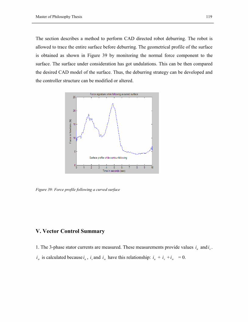
Kashikar, P. (2014) Control of the interaction of a gantry robot end

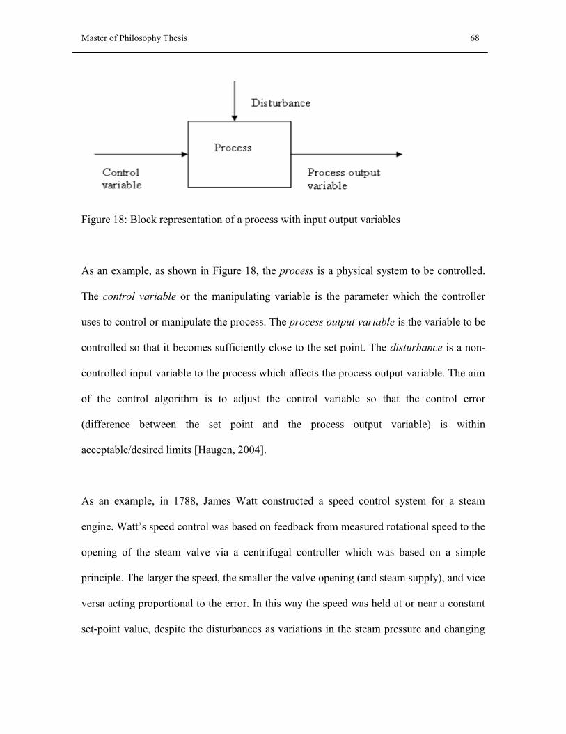
effector with the environment by the adaptive behaviour of its joint

drive actuators. MPhil, University of the West of England. Availablefrom: http://eprints.uwe.ac.uk/24857

We recommend you cite the published version.The publisher’s URL is:http://eprints.uwe.ac.uk/24857/

Refereed: No

(no note)

Disclaimer

UWE has obtained warranties from all depositors as to their title in the materialdeposited and as to their right to deposit such material.

UWE makes no representation or warranties of commercial utility, title, or fit-ness for a particular purpose or any other warranty, express or implied in respectof any material deposited.

UWE makes no representation that the use of the materials will not infringeany patent, copyright, trademark or other property or proprietary rights.

UWE accepts no liability for any infringement of intellectual property rightsin any material deposited but will remove such material from public view pend-ing investigation in the event of an allegation of any such infringement.

PLEASE SCROLL DOWN FOR TEXT.

http://eprints.uwe.ac.uk/24857/

Control of the interaction of a gantry robot

end effector with the environment by the

adaptive behaviour of its joint drive actuators

PARIKSHIT KASHIKAR

A thesis submitted in partial fulfilment of the

requirements of the University of the West of England, Bristol

for the degree of Master of Philosophy

in the

Faculty of Environment and Technology

University of the West of England, Bristol

October 2014

Master of Philosophy Thesis 1

Abstract

The thesis examines a way in which the performance of the robot electric actuators can be

precisely and accurately force controlled where there is a need for maintaining a stable

specified contact force with an external environment. It describes the advantages of the

proposed research, which eliminates the need for any external sensors and solely depends

on the precise torque control of electric motors. The aim of the research is thus the

development of a software based control system and then a proposal for possible inclusion

of this control philosophy in existing range of automated manufacturing techniques.

The primary aim of the research is to introduce force controlled behaviour in the electric

actuators when the robot interacts with the environment, by measuring and controlling the

contact forces between them. A software control system is developed and implemented on a

robot gantry manipulator to follow two dimensional contours without the explicit

geometrical knowledge of those contours. The torque signatures from the electric actuators

are monitored and maintained within a desired force band.

The secondary aim is the optimal design of the software controller structure. Experiments

are performed and the mathematical model is validated against conventional Proportional

Integral Derivative (PID) control. Fuzzy control is introduced in the software architecture

to incorporate a sophisticated control. Investigation is carried out with the combination of

PID and Fuzzy logic which depend on the geometrical complexity of the external

environment to achieve the expected results.


Acknowledgement

Thanks to the University of West of England (UWE), Bristol for giving me the opportunity

to carry out the research work. My debt of gratitude to Mr. Farid Dailami for being of

constant help and support to me, for guiding perfectly my work on this thesis from the very

beginning – with his precious ideas, advice and remarks, his words of encouragement and

motivation, when I needed them the most.

I like to express my sincere gratitude to my Director of Studies, Dr. Anthony Pipe, and Dr.

Quan Zhu for all their efforts, encouragement and support during the entire thesis work.

Thanks to all of the supervisory team –each of them for having a desk with knowledge,

experience and vision -without which it would not have been possible.

Thanks to Mr. Terrence Blake, Mr. David Worgan, and Mr. Gary Slocombe for the

experimental aspect of the research work, and their guidance and unstinting help. Thanks

to all my past and present colleagues and friends at UWE, Bristol, where I studied and

worked for more than six years, in a wonderful atmosphere of team spirit, union and

friendship. All of you that I have probably forgotten to thank here.

Most importantly I would like to dedicate the thesis to my parents for their endless and

tireless support, encouragement and blessings. I would also like to thank J. Hierl for his

strong support and encouragement.

Parikshit Kashikar.


Contents

Abstract .......................................................................................................... 1

Acknowledgement ......................................................................................... 2

List of figures: ................................................................................................ 6

Terminology and Nomenclature used in the presented work: ................. 8

Thesis Structure and Summary ................................................................. 11

1. Introduction .......................................................................................... 14

1.1 Introduction and Motivation of the Research ......................................................... 14

1.2 Research Objectives ............................................................................................... 16

1.3 Adopted Research Strategy .................................................................................... 17

2. Literature Survey .................................................................................... 20

2.1 Introduction ............................................................................................................ 20

2.2 Literature review .................................................................................................... 21

2.3 Introduction and Justification of the research undertaken ...................................... 27

2.4 Application Areas ................................................................................................... 31

3. Mathematical modelling of the electric actuator (PMSM) for the

controlled interaction with environment .................................................. 36

3.1 Mathematical representation of a PMSM ............................................................... 37

3.2 Introduction to spring like behaviour in electric actuators ..................................... 43

4. Development of the experimental setup for robot interaction with the

environment and initial tests ...................................................................... 45

4.1 Introduction of the system ...................................................................................... 45

4.2 Description of the control system architecture, electrical actuator and controller . 46


4.3 Data acquisition, interpretation and utilisation in the controller ............................ 50

4.4 Calibration of motor current to force experiment .................................................. 55

4.5 Development of the system and initial robot interaction experiments ................... 57

4.6 Approach to development of contour following system ........................................ 59

4.7 Software development flow charts ......................................................................... 60

5. PID control modelling and implementation on the experimental system

....................................................................................................................... 67

5.1 Background and Introduction ................................................................................. 67

5.2 Introduction ............................................................................................................ 69

5.3 Approach to the development of the PID controller .............................................. 74

5.4 Modelling and validation of the controller ............................................................. 75

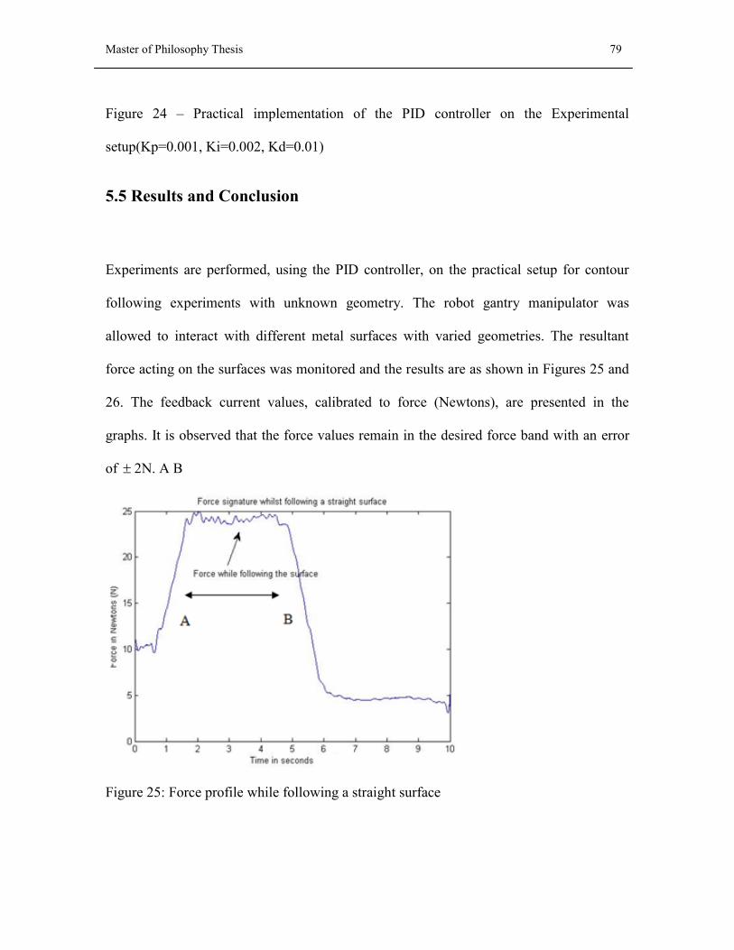
5.5 Results and Conclusion .......................................................................................... 79

5.6 Further Development with PID Controller ............................................................. 80

6. Development and Implementation of Fuzzy Logic Controller on the

experimental system .................................................................................... 82

6.1 Introduction and Justification for the need of fuzzy controller. ............................. 82

6.2 Approach adopted in designing the fuzzy controller .............................................. 84

6.3 Implementation and Tests ...................................................................................... 89

6.4 Comparison between the performance of PID and fuzzy controllers .................... 92

6.5 Proposed modified controller structure for PID+Fuzzy Controller........................ 96

7. Main Contributions and Conclusions of the research ......................... 99

8. Recommendations for future work ..................................................... 103

References and Bibliography ................................................................... 106

Appendices: ................................................................................................ 114

I. DSP TMS320F2812 Introduction- .......................................................................... 114


II. Infranor Amplifier: .................................................. Error! Bookmark not defined.

III. Introduction and operation of PWM in the amplifier of the motor ...................... 116

IV. PID Control Appendix ......................................................................................... 117

V. Vector Control Summary ...................................................................................... 119

VI. Description of coordinate transforms .............................................................. 121

VII. Mathematical derivations for torque control in PMSM ...................................... 123

VIII. DSP Software code- .......................................................................................... 126

a. Program for the X axis controller for conventional PID controller ........................................................ 127 b Program for the Y axis controller for conventional PID controller ........................................................ 137 c. Program for the X axis controller for fuzzy controller .......................................................................... 145


List of figures:

Figure 1: Permanent magnet synchronous motor (PMSM)……………………… 37

Figure 2: A Generic gantry manipulator layout……………………………………..45

Figure 3: Control system architecture employed in the research…………… 46

Figure 4: Block diagram of Vector control of an AC motor ………………………47

Figure 5: Block diagram of the control system architecture implemented for a single robot

axis………………………………………………………………………………… 52

Figure 6: Robot manipulator………………………………..………………………..53

Figure 7: Two arms of InFACT…………………………...………………………….66

Figure 8: robot electric actuator and manipulator……………………………. 53

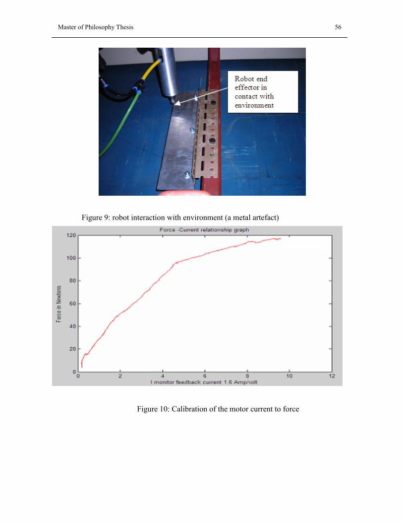
Figure 9: robot interaction with environment ………………………………………55

Figure 10: Calibration of the motor current to force ……………………………..55

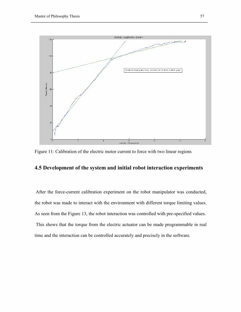
Figure 11: Calibration of the electric motor current to force with two linear regions..57

Figure 12: Graph showing torque/current limiting values over 10 seconds interval. 57

Figure 13: The force vector components and ft and the resultant force vector.. 58

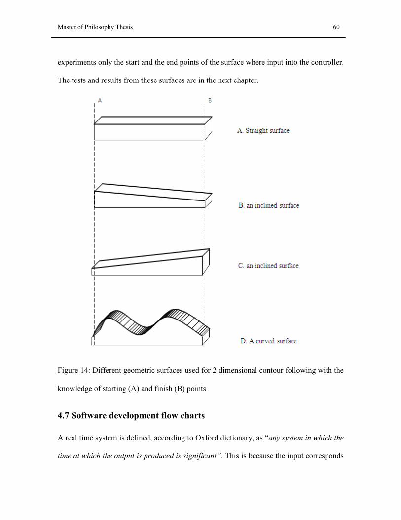
Figure 14: Different geometric surfaces used for 2 dimensional contour following with the

knowledge of starting (A) and finish (B) points………………………………….. 59

Figure 15: Flowchart describing robot electric actuator with the environment…. 61

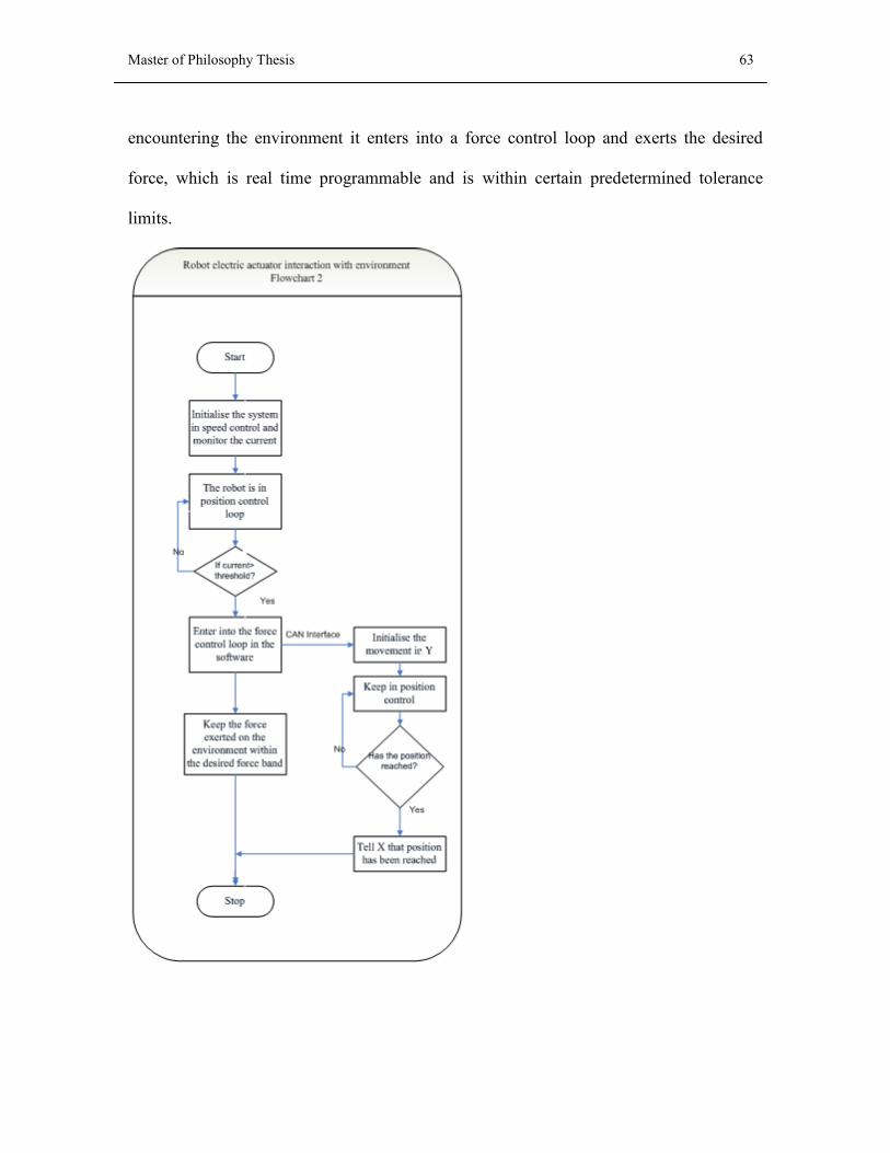
Figure 16: Flowchart describing robot electric actuator with the environment for two

dimensional surfaces…………………………………………………………. 63


dimensional surfaces………………………………………………………… 65

Figure 18: Block representation of a process with input output variables ………67

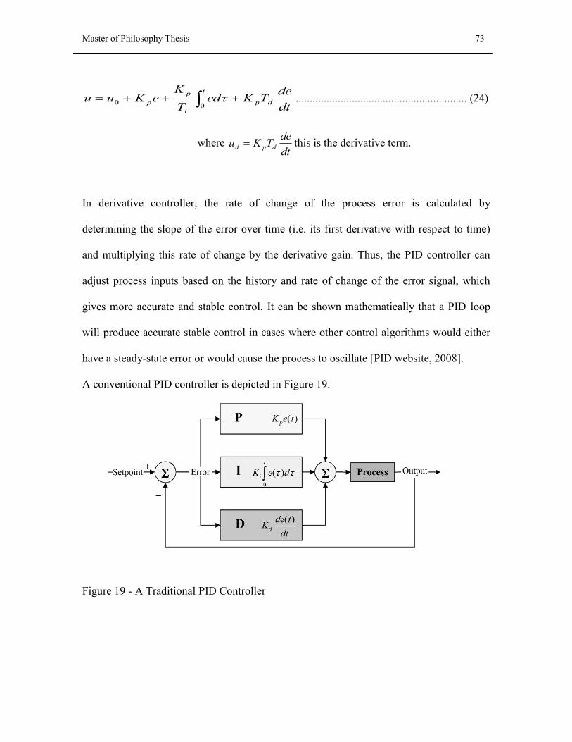
Figure 19 - A Traditional PID Controller…………………………………... 72

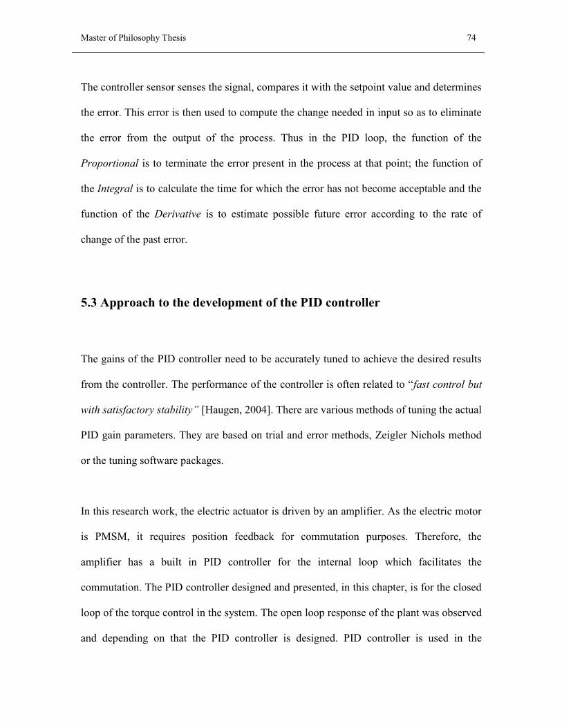
Figure 20: Different values of ζ calculated from the step inputs to the plant……..…..76

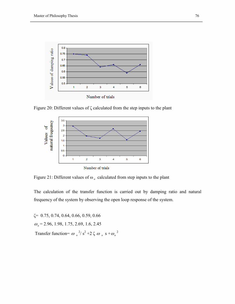
Figure 21: Different values of ω calculated from step inputs to the plant………..76

Figure 22– Simulink model for the PID controller implementation and comparison with

plant open loop response. (Kp=1.4, Ki=2.8, Kd=0.18)…………………….. 76

Figure 23 - Graph showing the Simulink plant output with and without PID control…78

Figure 24 – Practical implementation of the PID controller on the Experimental

setup(Kp=0.001,Ki=0.002,Kd=0.01)………………………………………………………79


Figure 25: Force profile while following a straight surface………………………….79

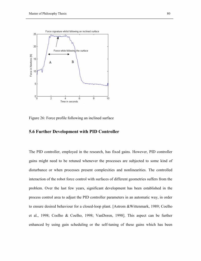
Figure 26: Force profile following an inclined surface………………………………..80

Figure 27: Example of membership functions……………………………….. 84

Figure 28: Fuzzy logic membership functions example…………………….. 84

Figure 30: Design of the Fuzzy Controller for 2D surface following………………..89

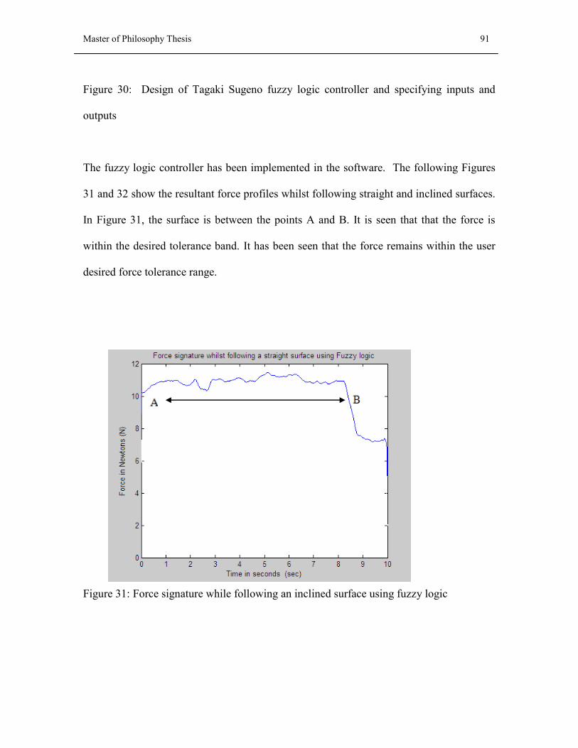
Figure 31: Design of Tagaki Sugeno fuzzy logic controller and specifying inputs and

outputs ………………………………………………………………………………90

Figure 32: Force signature while following an inclined surface using fuzzy logic…

………………………………………………………………………………91

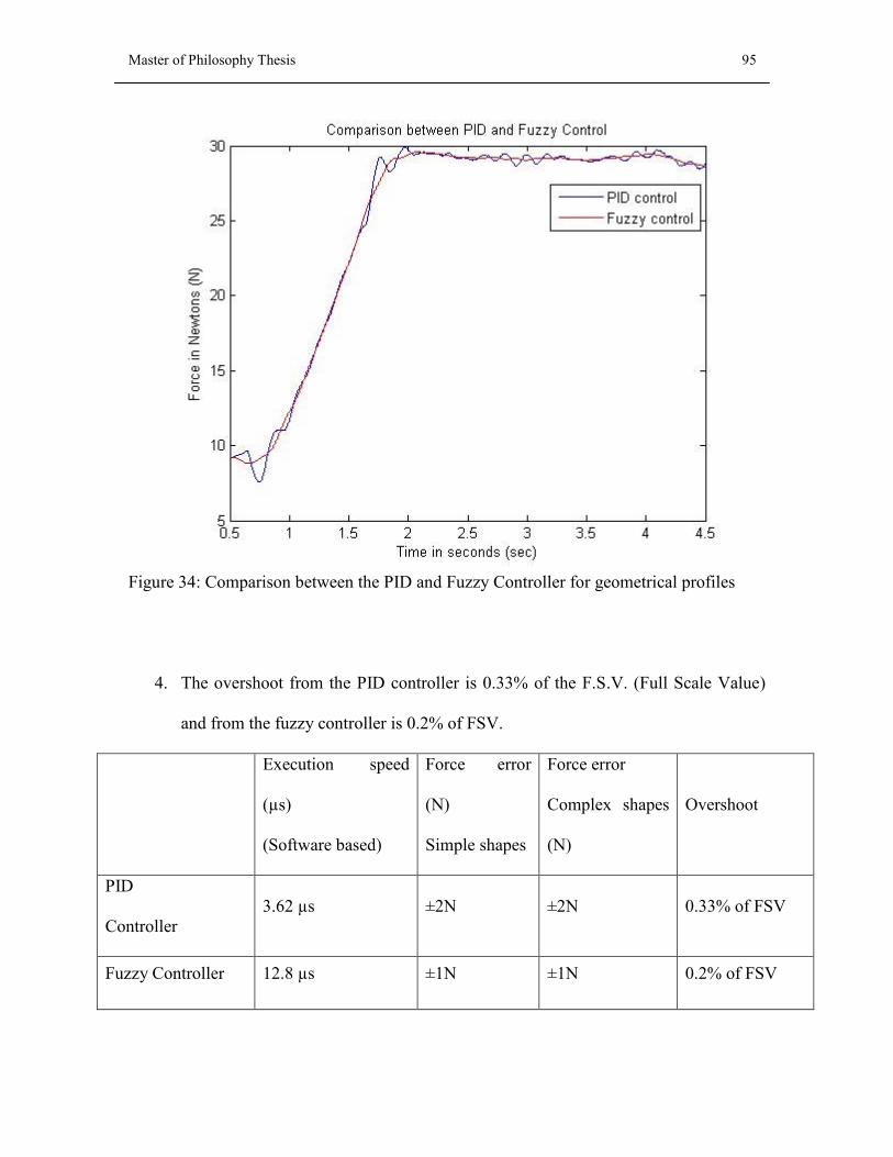
Figure 33: Comparison between the PID and Fuzzy Controller for geometrical profiles

………………………………………………………………………………93


………………………………………………………………………………94

Table 35: Performance comparison between PID and Fuzzy Controller on the experimental

rig ……………………………………………………………………………….95

Figure 36: Modified Controller structure for PID+Fuzzy controllers……… 97

Figure 37: Profile of the surface following using the modified control strategy… 97

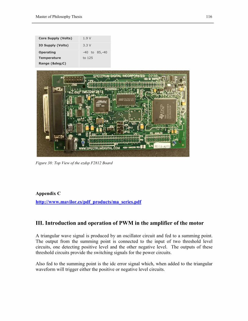
Figure 38: Top View of the ezdsp F2812 Board…………………………….. 115

Figure 39: Force profile following a curved surface……………………….. 121

Figure 40: Stator and rotor flux linkages in different reference frames…….. 128


Terminology and Nomenclature used in the research work:

qV : q axis stator voltage

: flux linkage

q : q axis flux linkage

iu : Integral term

iT : integral time

pK : proportional gain

s : amplitude of stator flux linkage

convK :constant used for force to torque conversion

d : the d axis flux linkage

dI : d axis stator current

dV : d axis stator voltage

eT : electromagnetic Torque

qI : q axis stator current

f : rotor flux linkage

sR :stator resistance

L : stator self inductance and with the d and q subscripts represents inductances for those

axes

e :control error

F : force exerted by the robot on the environment.

du : derivative term

dT :derivative time

0u : nominal value of control variable

pu :Proportional term

P : number of poles

p : differentiation operator d/dt

u : control variable


δ : angle between stator and flux linkage

ω : electrical angular velocity of the rotor

*r

dsi,

*r

qsi,

r : inputs to the inverse Park transform as described in Chapter 4

*

ui*

vi*

wi : outputs to the inverse Clarke transform as described in Chapter 4

*

dsi *

qsi: inputs to the inverse Clarke transform as described in Chapter 4

r

dsi r

qsi :outputs to the Park transform as described in Chapter 4

qsi dsi: inputs to the Park transform as described in Chapter 4

dsi qsi: outputs to the Clarke transform as described in Chapter 4

ui vi : inputs to the Clarke transform as described in Chapter 4


Abbreviations:

AC motor : Alternating Current Motor

ADC :Analog to Digital Converter

BIT: Bristol Institute of Technology

B : Damping of the mechanical spring

CAN: Controller Area Network

CCS :Code Composer Studio Software environment

CFRP : Carbon Fibre Reinforced Plastic

CMM : Coordinate Measurement Machine

CNC : Computer Numeric Control

DAC :Digital to Analog Converter

DC: Direct Current motor

DSP : Digital Signal Processing

FL: Fuzzy Logic

FSV :Full Scale Value

GPIO: General Purpose Input Output

InFACT: Integrated Flexible Assembly Cell Technology

IO: Input/Output port

K : mechanical spring constant

MIMO: Multi Input Multi Output

P : Proportional controller

PC: Personal Computer

PI: Proportional Integral controller

PID: Proportional Integral Derivative Controller

PMSM: Permanent Magnet Synchronous Motor

PWM: Pulse Width Modulation

RCC: Remote Centre Compliance

SISO: Single Input Single Output system

SPI: Serial Peripheral Interface bus

TI: Texas Instruments


Thesis Structure and Summary

Chapter 1: Introduction:

In this chapter, introduction of the research is described. Afterwards the

motivations, research objectives of the presented work are explained to aid the

reader.

Chapter 2: Literature Survey:

This chapter explains the specific field of research to which this work relates to. It

explains the justification and the inspiration of the work undertaken. The detailed

explanation is carried out of the potential application areas of the proposed control

philosophy.

Chapter 3: Mathematical representation of the PMSM:

The mathematical representation of the PMSM is described in this chapter which

forms the basis of the proposed control philosophy for the electric actuators. The

chapter also describes the introduction of the force controlled behaviour in the robot

joint drive actuators.

Chapter 4: Development of the experimental setup:

The chapter begins with the description of the experimental setup used in the

research. It describes the data acquisition and interpretation of the controller signals.

The calibration experiments related to force exerted on the environment and the

motor current is described in this chapter. The initial basic development is explained

with the aid of software flow charts for contour following experiments.


Chapter 5: Development of PID Controller:

This chapter gives an introduction and justification for the PID controller. The

chapter then explains the modelling and implementation of the PID controller on the

robot gantry experimental setup. The tests are conducted on the experimental setup

for contour following applications.

Chapter 6: Development of Fuzzy logic controller:

This chapter presents the justification for the introduction of Fuzzy controller in the

software for torque control on the present experimental rig. The chapter describes

the approach adopted in the design of the fuzzy controller. The fuzzy controller is

designed and implemented on the experimental setup for torque control. The tests

and results are presented and compared with PID controller. The research work is

then focussed on the design of controller using both the PID and the fuzzy controller

for interaction with complex geometrical contours.

Chapter 7: Main Contributions and Conclusions:

This chapter presents the main contributions of the most salient points made

throughout the thesis, along with the examination of how the work undertaken has

addressed the issues raised in the research questions.

Chapter 8: Future Work:

Fruitful ideas for future work are identified and are discussed further in this chapter.

Some new areas are depicted- some are future-work while the rest are modifications

of the existing research work.


Appendices:

The appendices provide an abundance of ancillary information for the project.

Whilst the main chapters explore the theoretical background and results of practical

tests, the appendices provide more practical aspects of the research such as the

controller introduction and its operation and the entire software code for the

undertaken research work.


Chapter 1

1. Introduction

1.1 Introduction and Motivation of the Research

Automation (ancient Greek: self dictated) or industrial automation or numerical control is

the use of control systems such as computers, to control industrial machinery and

processes, reducing the need for human intervention [Dictionary Reference, 2008]. Robot

automation plays an increasingly important role in industrial applications and global

economy. Engineers strive to combine automated devices with mathematical and control

tools to create complex systems for a rapidly expanding range of industrial applications.

Robot automation improves quality, speed, production and cost. It has found numerous

applications in material handling applications such as pick and place, packaging, and

robotic assembly and manufacturing applications such as polishing, deburring, spot

welding and grinding.

Robotics has matured as a system integration engineering field defined by M. Bradley as

“the intelligent connection of the perception to action”. Programmable robot manipulators

provide the “action” component. A variety of sensors and sensing techniques are available

to provide the “perception” of the interaction with the environment [Petriu et al, 2008].

The industrial robot applications such as cranking a wheel, twisting a screw or deburring a

machined part require the robot end effector to physically interact with an external surface


or object. This interaction is aided with elastic pads or springs inserted in the robot end

effector or sensors such as position sensors, vision sensors, force sensors, proximity

sensors. The insertion of springs or elastic pads aids to limit the interaction forces between

the robot end effector in order to avoid damage to the surface or object in deburring,

polishing applications. The position, vision, force sensors are used to give feedback to the

robot controller and therefore the controller can take appropriate actions to bring about the

required motion in the electric actuators of the robot arm, and thereby in the robot structure,

to attain the desired outcomes.

There is an inherent disadvantage in the inclusion of the sensors in the robot controller

structure. The acquisition, interpretation and utilization of the sensory information in the

controller can affect the responsiveness of the robot to external changes. Another

disadvantage is the cost and unsuitability to adapt to different working conditions. The

different working environments also demand compliance in the traditionally stiff robot

structures. This is important so that the interaction of the robot end effector with the

environment can be controlled precisely and accurately. Compliance can be introduced in

an active or a passive manner in the robot structure. The use of mechanical springs or

elastic pads is termed as a passive manner of introducing compliance. This method has

limited performance and lack of adaptability to different applications. The amalgamation of

pneumatic system in the robot end effector introduces active compliance in the system but

the cost, difficulty of control remains the main drawbacks.

Robot applications such as grinding, surface finishing operation like deburring require the

robot position control as well as force control and it becomes a complex Multi Input Multi


Output (MIMO) system. The research focuses on the inherent architecture of the robot

without any additional or subordinate sensors connected to the robot. The aim is the precise

and accurate control of the robot joint electric motors and introduction of active compliance

in the system. The performance of the electric motor is varied in accordance with the

environmental constraints. The motor current is used as an indicator for torque and shaft

encoder data provides the necessary feedback information to enable motor control to be

exercised. Thus the robot interaction with external object or surface is made programmable

in real-time applications. The advantages are less cost, less acquisition and the utilization

for the interpretation of force information and the varied performance based on external

conditions or desired applications.

The outcome of the research can be applied to processes such as assembly, grinding,

deburring and potentially coordinate measurement systems. The experimental work is

carried out on a permanent magnet synchronous motor. The experimental work can also be

extended to both permanent magnet and brushless DC motors.

1.2 Research Objectives

To develop a software based controlled behaviour in the joint electric actuator so

that the interaction of the actuator, and thereby the robot, is made programmable in

real time applications and to exhibit this behaviour when the robot interacts with the

environment.

To develop and implement software architecture for a two dimensional contour

following force control strategy based on the accurate torque control of the electric

actuators of the robotic system.


To engineer the robot force control system that will traverse two dimensional

artefacts without previous geometrical knowledge and within a configurable force

deviation tolerance range.

To design and validate control strategies such as the conventional PID control and

fuzzy control to obtain a stable, accurate and reliable system; controller selection

being based upon the optimum performance under various operating conditions.

To provide a survey of various research and manufacturing areas where this

innovative control strategy can be applied.

1.3 Adopted Research Strategy

The experimental studies of the research are carried out on a robot gantry manipulator at

the University of the West of England (UWE), Bristol. A generalised study and inspection

is carried out on the rig. The electric actuator used in the research is a Permanent Magnet

Synchronous Motor (PMSM) but the control philosophy demonstrated is applicable to

other electric actuators. The research is focused on automation of manual deburring

although it can be extended to other applications. A broad literature survey is performed.

An experimental study is also carried out with a force sensor connected to a robot arm and

to compare its results with the proposed control philosophy.


Design and implementation of the controller and data acquisition boards is carried out and

introductory experiments are conducted on the test rig for two dimensional contour

following. Calibration experiments are performed on the experimental setup for torque-

force relationship.

A two dimensional contour following robotic system based on torque control of the

electric actuator is designed and implemented for surfaces with unknown geometry.

The data acquisition, which included, current feedback is employed on practical

experimental setup. Contour following experiments were carried out on different surfaces

with unknown geometry.

Mathematical representation of the electric actuator is carried out and is validated on the

rig to demonstrate force control behaviour in the real actuator. The force control of the

actuator is made programmable so it exhibits active compliance.

PID controller design and implementation is carried out to give a stable, reliable and

repeatable robotic system. Simulation studies are performed and validated on the

experimental setup.

With an aim to incorporate control strategies for complex environments for automation

applications like deburring, fuzzy control is considered and tested. A switching

mechanism is developed between the conventional PID and fuzzy controller and,

depending on the environment conditions; a combination of both the controllers can be

used.


The research carried out is focussed on automation of robotic deburring but this research

can be extended to various other robotic applications. Therefore, a detailed research

survey was performed, to identify the possible application areas of the control philosophy.


Chapter 2

2. Literature Survey

2.1 Introduction

A robot is defined in many ways: "A reprogrammable, multifunctional manipulator

designed to move material, parts, tools, or specialized devices through various

programmed motions for the performance of a variety of tasks" [Robot Institute of

America definition, 1979]. "An automatic device that performs functions normally

ascribed to humans or a machine in the form of a human." [Webster Dictionary]. The first

definition is restricted to what a robot manipulator is doing in a mechanical sense. The

second definition is more general but still limited to what robots are supposed to do.

The basic idea of a practical robot is to replace humans in repetitive, dangerous, or tiring

tasks. As these repetitive, tiring jobs were found on production lines in industries,

Industrial robots were the first real beings to enter our world as operating machines. Cars,

electronic devices to consumer home appliances today are manufactured by automated

machines or “industrial robot” that replace the common worker in the production line.

An industrial robot manipulator is constituted of:


1. A mechanical structure or manipulator that consists of a sequence of rigid bodies

(links) connected by means of articulations (joints); a manipulator is normally

characterized by an arm that ensures mobility, a wrist that confers dexterity, and an end

effector that performs the task required of the robot.

2. Actuators that set the manipulator in motion through actuation of the joints, the motors

employed are typically electric or hydraulic, and occasionally pneumatic. Actuators are

needed to perform motion or manipulation in the external world.

3. Sensors that measure the status of the manipulator and, if necessary, the status of the

environment.

4. A control system (normally a computer) that enables control and supervision of

manipulator motion.[Sciavicco et al, 2000].

2.2 Literature review

Traditional/Conventional industrial robotic tasks, which are generally related to

manipulation or assembly, require only control of the position of the robot arm. The

managing of the robot interaction with the environment by adopting a purely motion or

position control strategy turns out to be inadequate for tasks like grinding, deburring or

composite layouts. Implementation of all these tasks intrinsically necessitates that a robot,

besides realizing the predisposed position, provides the necessary force to either

overcome the resistance from the environment or to comply with the environment. Also,

the unavoidable modelling errors and uncertainties in these applications may cause a rise

of the contact forces ultimately leading to an unstable behaviour of the robot arm during

the interaction [Zeng, 1997].


During the early work on telemanipulation, the use of force feedback was introduced to

assist the human operator in the remote handling of objects with a slave manipulator.

More recent research has been conducted on cooperative robotic tasks have been

implemented such as fingers of a dexterous robot hand where the robot force control is of

crucial importance as it has to limit the exchanged forces and avoid squeezing of a

commonly held object. Robot force control is used widely because autonomous field

robots for heavy industry must be rugged and reliable. Force control in industrial robotics

has been a key research area to increase robot performance and to introduce new

functionalities for the last 30 years and has been documented in research articles. Also, in

robot force feedback for deburring and grinding tasks and automated solutions have been

proposed and implemented. [Raibert and Craig, 1981, Siciliano and Villani, 2001,

Brogardh, 2007 Lu et al, 1992 Aertbelien et al, 1999]

Precise position and force control is required for applications such as assembly of

precision-component systems, grinding and deburring. A classification of robot force

control algorithms based on application of the relationship between position and applied

force or between velocity and applied force, or the application of direct force feedback, or

their combinations includes:

methods involving the relation between position and applied force;

methods applying the relation between velocity and applied force;

methods applying directly position and applied force: hybrid position / force

control, and hybrid impedance control;

methods applying directly applied force feedback: explicit force control.


[Salisbury, 1980, 1982, Borrel, 1979, Whitney, 1977, 1987, Colbaugh, 1992, Mason,

1981, Raibert, 1981]

The two basic approaches to force control are Hybrid and Impedance control [Hogan,

1985]. Hybrid control [Raibert, 1981] is based on the decomposition of the workspace

into purely motion controlled directions and force controlled directions. In Hybrid

control, both a motion controller and a force controller are implemented but the force

controller is given precedence. The insertion of a peg in a hole can be achieved using

hybrid force decomposition. The position error is changed proportionally to the equivalent

force error in the working space first. This is transformed to joint torque error and then

fed to the controller. The controller also compensates for the friction force. The force can

be applied to a direction orthogonal to the position control [Raibert, 1981]. Impedance

control is similar to pure position control where a desired velocity is commanded, except

that the impedance of the robot is regulated to avoid excessive force build-up. Impedance

control [Hogan, 1985] does not regulate motion or force directly but regulates the ratio of

force to motion which is the mechanical impedance.

Impedance control is robust while making contact with unknown surfaces. Hybrid control

has to be divided into two modules: one for free space motion and the other for impact

transition for dealing with unknown surfaces. The advantage of a hybrid controller over

Impedance control is that the contact force can be regulated accurately [Hogan, 1985

Schutter, 1997 Raibert, 1981 and Sung-Hyun Han, 1999]. In the presented work, Hybrid

force controller has been used and the force and motion control strategies are separate in

the control system architecture.


To achieve robot force control, the adoption of sensors is of crucial importance to achieve

high-performance robotic systems. These are divided into two classes: proprioceptive

sensors and heteroceptive sensors. The former are joint position, joint velocity and joint

torque sensors which measure the internal state of the manipulator while the latter are

force sensors, proximity sensors, range sensors and vision sensors that provide the robot

with knowledge of the surrounding environment. The goal of these sensors is to extract

features characterizing the interaction with environment, thus enhancing the degree of

autonomy of the system. Sensing is particularly difficult because industrial environments

are often dirty, dusty and noisy, both acoustically and electromagnetically. For these

conditions, force sensing is one of the most appropriate technologies, because it is

relatively insensitive to these factors, is well developed and economical. This force

information is used for path modifications in the robot controller to achieve the desired

operation [Sciavicco et al, 2000].

Robot interaction with the environment can be controlled by the inclusion of sensors

which feedback the force data. The force signals are used in a path trajectory controller to

make the required changes in the robot path. It is crucial to adhere to the required forces

on the environment, otherwise too much force could damage the surface/environment or

too little force could not give the desired results perhaps even losing contact with

environment. One solution is to have a mechanical device (remote centre of compliance)

interposed between the manipulator end effector and the environment which has high

stiffness in one direction and high compliance in the other directions, which can avoid

excessive force build-up. This is termed passive compliance. The disadvantages of this


method are rigidity of the device, cost, and failure to adapt to different environments.

Therefore, another solution is preferred where the force acting on the environment can be

monitored in real time and the robot can comply with either the desired trajectories or set

force bands. This is active compliance [Siciliano & Villani, 2001].

Force sensors usually consist of an array of strain gauges which delineate the linear and/or

rotational components of the vector force along the three/six axes of the sensor coordinate

frames [Sponge, 1989]. Measurement of force and/or torque is usually reduced to

measurement of the strain induced by the force (torque) applied to an extensible element

of suitable features. Therefore, an indirect measure of force is obtained by means of

measurements of small displacement. The basic component of a force sensor is the strain

gauge which uses the change of electric resistance of a wire under strain. The strain gauge

is constituted by a wire of low temperature coefficient. The wire is disposed on an

insulated support which is glued to the element subject to strain under the action of stress.

As dimensions of the wire change, they cause a change of electric resistance. Design

parameters are chosen in such a way that the resistance changes linearly in the range of

admissible strain for the extensible element. To transform changes of resistance into an

electric signal, the strain gauge is inserted in one arm of a Wheatstone bridge which is

balanced in the absence of stress on the strain gauge itself.

The sensor type which has gained a lot of industrial and academic attention is the six axis

force/torque sensor. The sensor is used widely in industrial applications with increased

product quality and reliability. However, the force sensors, in general, have some

drawbacks. The programming and tuning methods need further development [Brogardh,


2007].The speed of response; in particular can have a significant effect on the efficacy of

this approach. Also, force sensors are expensive, can be damaged whilst in operation. The

force data from the sensor needs to be acquired, modified and then utilised in the

controller structure which is difficult. Therefore, the precise utilisation of the force signal

becomes a crucial issue in these applications; otherwise it may lead to robot actuator

saturation or damaging the object/ work-piece.

Some research in robot force control focuses on using the position feedback and relating

the velocity with the force exerted on the environment. Thus, the position feedback is

calibrated to force values exerted on the environment and, in real time applications,

knowledge of the environment can be obtained by monitoring the robot position [Siciliano

& Villani, 2001]. In [H. Kawasaki et al, 2006], research has also been carried out without

using a force sensor but by observing the joint position and velocities of the robot arm.

Thus, research has been conducted on force feedback without a force sensor.

But in these researches, the inherent stiffness of the robot arm is not changed or altered.

This makes sense in traditional position controlled robot systems where high stiffness

reduces instability. But lower interface stiffness has advantages such as more accurate and

stable force control and less damage during inadvertent contact. This alteration in the

stiffness aids in the controlled interaction with the environment and improvement in the

compliant interaction [Schutter et al, 1986].


2.3 Introduction and Justification of the research undertaken

Automation of manufacturing tasks like deburring and polishing require introduction of

science into traditionally art based processes. The aim is to design and implement

complex behaviour in the control structure. This is introduced in a robotic system or a

Computer Numerical Control (CNC) machines by force control strategies. The force

control methods can be broadly implemented as rigid structures and compliant structures.

With conventional rigid structures/tools it is very difficult to control the interaction with

an object/surface.

Compliance is the ability of an object to yield elastically or in a spring like manner when

subjected to a force. Compliance control is very important and it is normally introduced in

the system with the addition of external sensors such as mechanical springs and

pneumatic actuators which are unadoptable to different geometrically varying surfaces

and difficult to control respectively.

Adaptive force control is crucial during this interaction as the operation demands the

alteration of the performance during the process execution. An example is the need for the

increased grip force when pressing against a spring as more force is required as the spring

is compressed. Another example of adaptive control is the application of more power to a

motor to maintain a constant speed, as when a robot moves from a level ground to an

incline or when it tries to move a heavy object.


This research aims to provide this type of adaptive compliant behaviour in an electric

actuator attached to a mechanical system without the above mentioned external sensors.

The goal of the research is the control of the electric actuator wherein a stable and

specified contact force with the environment is to be maintained. The research work aims

to develop this innovative approach by the control of electric actuators. Instead of

generating this force data through a mechanical and rigid force sensor, force information

can be obtained from the electric actuators (PMSM) driving the robot arm.

Brushless AC servo drives are increasingly used in high performance positioning systems

such as robots and manipulators because of their excellent parameters compared to

conventional DC motors or induction motors. The power density of a PMSM is higher

than the induction motor due to the fact that there is no stator power dedicated to magnetic

field production. These motors are controlled by techniques such as Vector control. In this

method, the position feedback from the motor rotor is required to transform the three

phase variable into two phase axes frame in the synchronously rotating reference frame

aligned with the rotor flux linkage vector. This is done to maximise the torque supplied by

the motor. Research on the control and performance of PMSM has been carried out and

documented in articles. [Schutter et al,1986, Kaewjinda, 2007 and Pillay et al, 1988, 1989,

Vector control, NEC application notes, 2002]. Research has been done on the precise

modelling and method of operation of PMSM [Pillay et al, 1988, 1989]. In [Hyungbinet

al], the dynamic behaviors of a BLDC motor are analyzed, when the motor undergoes

mechanical and electromagnetic interaction due to an air gap variation between the stator

and rotor and thereby controlling the torque.


The motor current reflects the torque of the actuator and thereby the force of the system

[Sponge et al, 1989]. The torque of the motor can be altered depending on the load on the

system and hence the force exerted by the system. Thus, the motor current can be

calibrated to reflect the force exerted by the manipulator on the environment. By

achieving this, we are able to introduce active compliance in the system. The robot

interaction with the environment can be made programmable and the force exerted can be

changed. Thus, the electric actuator behaves as a programmable spring. The contact force

depends on the robot joint actuator stiffness. The stiffness can be varied to yield elasticity

or a spring like behaviour when a force is applied, thereby introducing compliance in the

system. Therefore, the need for an external force sensor is avoided.

Using an adaptive controller for real time applications like grinding and deburring

requires a powerful processor. Nowadays, the development of new materials, the

improvement in the mechanical design of robot manipulators and faster microprocessors

have highlighted the necessity of applying more sophisticated control algorithms in the

new generation of industrial robotics [Siciliano and Villani, 2001]. An adaptive controller

continuously tracks plant parameters and constantly, or periodically, modifies the

parameters of the control system to provide optimum performance. To achieve this, a

Digital Signal Processor (DSP) is required.

Significant research in intelligent and Adaptive control has been performed based upon

the PID control, fuzzy control and neural network approaches. PID controllers are

extensively used because of the advantageous properties they exhibit such as robustness,

simplicity and accuracy. However, due to non-linearities whilst dealing with the


environment, sometimes the preferred solution is fuzzy control or neural networks, which

aim to incorporate more complex behaviour and reasoning skills in the automation of

robot operations to handle non-linearities. Fuzzy control has become a popular approach

for performing the task of controller design because the human reasoning skills can be

incorporated in the controller structure. Therefore, fuzzy control is often applied to some

ill-defined systems. This explains the current trend in the theoretical development to

combine fuzzy control techniques with conventional PID control techniques to obtain

adaptive fuzzy control.

For example, in [Ahn et al, 2011] an online smart tuning fuzzy PID approach based on a

robust extended Kalman filter for the development of high force control precision is

presented, where force or position control with high accuracy is exceedingly necessary. In

[Hamit] a neurofuzzy controller has been used to linearlize the highly nonlinear sensor and

motor output signals.

In some cases, industrial robot operation demands high accuracy performance that is not

achievable by using a conventional PID control. In [Kaitwanidvilai, 2004], the concept of

switching between a PID controller and a neurofuzzy controller has been implemented on

a pneumatic system. The experimental results have confirmed that the concept of

multimode switching yields better results than classical control or the neurofuzzy

controller acting alone. Research has been documented in articles. [Trusca, 2003, Burn,

2003 Chang, 1999, Hassan, 2002].


2.4 Application Areas

Robot force control can be used for various robot automated operations like polishing,

assembly and deburring. The automation of the preceding mentioned applications is often

restricted because of the complexities associated with the applications. Therefore, in some

cases, manual work option is still given precedence to automated operations. The research

can be applied to these applications because the performance of the robot electric actuator

can be varied in real time in accordance with the environmental constraints. This proposed

control philosophy aims to include these complexities and non linearities in the adaptive

control structure.

Automated Deburring applications-

A burr is a sharp and raised edge that is formed in several manufacturing processes such

as milling, drilling, turning and other machining operations. These burrs have to be

removed for ergonomic, aesthetic, and/or functional reasons. A small series of large

components pose a problem and are most often manually cleaned with a grinding tool.

Manual deburring techniques have disadvantages such as poor working conditions,

production delays and inconsistent work quality. The robot should have a stable force

control throughout the entire machining process. Automation normally requires the

detailed knowledge of the environment beforehand. Automated robot deburring systems

are becoming crucial as the cost of manual deburring can be around 30-35% of overall

production costs [Murphy, 1990 Hsu, 2000]. Several problems prevent a breakthrough in

this area which includes variations in the work piece position which are unavoidable

without expensive clamping and fixtures systems. These specially designed clamping


systems cannot be used on small series of components. Due to the nature of the processes

such as casting and forgings, work pieces commonly have high geometrical inaccuracies.

These factors limit the use of traditional position controlled robots. Other sensors can be

used to solve these problems. Force feedback is a good candidate, but its use necessitates

specific control strategies that depend on the type and size of the burrs, the materials of

the work-piece and grinding tool, and the task goals.

The presented work has been researched and implemented and can be applied to robotic

deburring. To achieve this goal, a cutting tool with a fixed spindle speed has to chamfer

the part edges while undergoing contour-following motion. While driving the cutting tool

to perform a deburring process, the deburring robot must implement two major motions.

One motion applies a suitable chamfering force to the part‘s edges to remove the burrs

while avoiding damage to the part. The other motion performs contour following. This

ensures the cutting tool remains in contact with all the burrs over the chamfer by

appropriate torque control. A heuristic deburring control policy can attain the desired

chamfering force by controlling the feed-rate of the cutting tool. The heuristic policy

simply consists of slowing down the feed-rate of the cutting tool when the encountered

burr is large, and speeding it up if otherwise [Kazerooni, 1987, Lu et al, 1992 Hsu Feng-

Yi et al, 2000].

Most industrial robots rely on teach programming, a process that is tedious and time

consuming. An alternative method uses Ccomputer-Aided Design (CAD) data and a

representation of the robot’s environment to compute manipulator coordinates off-line.

Unfortunately, robots usually have insufficient accuracy to use off-line programming


alone, and it is ineffectual without on-line modification. Finally, for a work piece with

partially unknown contours, planning a trajectory may be infeasible. An alternative

approach could be to use accurate on-line trajectory teaching via the work piece’s surface

geometry; a roller bearing, or a properly designed jig, is mounted on the robot end-

effector. However, these machines are very expensive and frequently cost too much to

justify their use in a deburring applications. Also, the mechanism is more complex [Seng

Chi-Chen et al, 1999, 2000].

Researchers have worked on automation of deburring and polishing on unknown

geometrical contours. Research has been done in these industrial operations but a majority

of them rely on the force signature from the additional mounted sensors on the end

effector [Garcia et al,2008, Seng Chi-Chen, 1999, 2000].

Coordinate measurement machines-

Another application is coordinate measuring machines. Coordinate measurement

machines (CMM) also demand a precise and accurate force and position control of the

component. The overall measurement time of the component can be reduced if the

actuators are introducing the compliance rather than at the probe used on the end of the

arm in CMM. The compliance behaviour in the electric actuators will allow a certain

specified position error to develop between the probe and the component to be measured.

This control philosophy can also been implemented in biomedical engineering research

involving automation of surgical procedures.


Composite layout force control-

The new Boeing B787 and Airbus A380 are seen as an indication of a step change in the

use of composites in commercial aviation. The aircraft industry is undergoing a rapid shift

to composite materials in the development programmes for new aircraft and is facing

what it calls a ‘historic expansion of demand for such materials’. The use of reinforced

plastic in aircraft has grown enormously since the early 1970. The challenge now is

increasing the use of this composite material throughout the aircraft in order to increase

durability, decrease weight (thus increasing fuel efficiency) [Airbus, 2007].

The composite material used in aircraft in layers, with adhesive applied in-between each

layer. The aerospace industry is producing composite material called Carbon Fibre Re-

enforced Plastic (CFRP) and a significant proportion of its manufacturing involves high

precision work performed by skilled labourers. Segments of the fuselage and the other

large artefacts are manufactured by existing robotic systems, but the more intricate,

complex geometrical shapes (aerodynamics) are considered to be outside the robot

capabilities. This is because the workers who perform these tasks possess skill, knowledge

and experience that arise from the intimate involvement with the environment and

involves very accurate force and position control. This is a complex non-linear,

multivariate control environment [Airbus, 2007].

The current research can be applied to these applications where compliance and stiffness

of the system are real time programmable and aims to include complex behaviour in these

automated robot operations. Thus, the presented research work focuses on the torque

control in the electric actuators which is then applied to follow unknown geometrical


contours with desired force values. Therefore, this novel control philosophy which

eliminates external sensors and also introduces spring-like behaviour in the electric

actuator of a robot is very beneficial to these above mentioned applications.


Chapter 3

3. Mathematical modelling of the electric actuator (PMSM) for

the controlled interaction with environment

Introduction

There is a vital interface between electrical and mechanical engineering. Wherever

mechanical motion is controlled by electronics, it is commonly referred to as a part of

“Mechatronics” [Miller, 1989]. Mechatronics involves control of mechanical motion

control systems in industrial, manufacturing and technological processes. The motion

control systems aim to achieve the specified performance demanded by users and industrial

standards in electric actuators [Lyshevski, 1999]. The electric actuator used in the research

work is a PMSM which requires a sophisticated electronic control, called Vector Control.

Motion control in Robotics is a long established and well understood field and forms the

basis of most modern manufacturing technology. The demand for high accuracy and

repeatability is traditionally achieved by employing high stiffness mechanisms with high-

fidelity sensors and control systems [Bigge et al, 2007].


3.1 Mathematical representation of a PMSM

The PMSM used in servo-mechanical systems is generally called “a brushless servomotor”

or “brushless AC servomotor” [Kaewjinda et al, 2007]. As results of the progress in power

electronics, software engineering, and materials, the PMSM, based on modern rare earth

magnet variety, has become a serious competitor to the induction motor and conventional

wound rotor synchronous motor. PMSM drives are used in many applications. They are

receiving increased attention because of their high efficiency, and small size. The PMSM is

preferred, in industrial servo applications, to the DC motor due to considerations of the

cost, size, low maintenance, maximum speed, capability, and simplicity of design. The

power density of a PMSM is higher than that of an induction motor with the same ratings,

due to no stator power dedicated to the magnetic field production. For this reason, they

have evolved into the preferred solution for speed and position control drives on machine

tools and robots. They are used in applications which require rapid torque control and high

speed operation [Zhong et al, 1997].


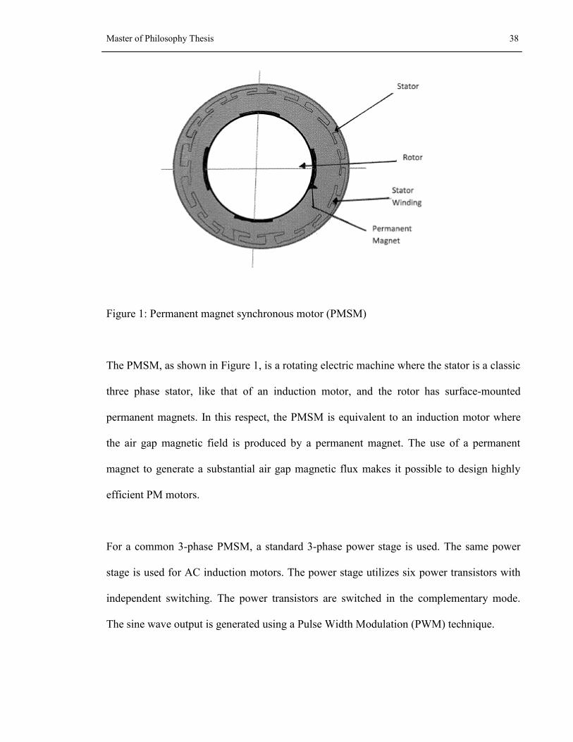
Figure 1: Permanent magnet synchronous motor (PMSM)

The PMSM, as shown in Figure 1, is a rotating electric machine where the stator is a classic

three phase stator, like that of an induction motor, and the rotor has surface-mounted

permanent magnets. In this respect, the PMSM is equivalent to an induction motor where

the air gap magnetic field is produced by a permanent magnet. The use of a permanent

magnet to generate a substantial air gap magnetic flux makes it possible to design highly

efficient PM motors.

For a common 3-phase PMSM, a standard 3-phase power stage is used. The same power

stage is used for AC induction motors. The power stage utilizes six power transistors with

independent switching. The power transistors are switched in the complementary mode.

The sine wave output is generated using a Pulse Width Modulation (PWM) technique.


A PMSM is driven by a sine wave voltage coupled with the given rotor position. The

generated stator flux, together with the rotor flux, which is generated by a rotor magnet,

defines the torque, and thus the speed of the motor. The sine wave voltage outputs have to

be applied to the 3-phase winding system in such a way that the angle between the stator

flux and the rotor flux is kept close to 90° to get the maximum generated torque. To meet

this criterion, the motor requires electronic control for proper operation, called Vector

Control. This is facilitated by the use of modern DSP and microcontrollers to attain the

functionality, flexibility and reliability required for the accurate torque control in electric

actuators.

Vector control is easily understood by forming a mental image of the coordinate reference

transformation process. If an AC motor operation is visualised from the perspective of the

stator, a sinusoidal input current applied to the stator is observed. This time-variant signal

generates a rotating magnetic flux. The speed of the rotor is a function of the rotating flux

vector. From a stationary perspective, the stator currents and the rotating flux vector look

like AC quantities.

The picture is visualised being inside the motor and running alongside the spinning rotor at

the same speed as the rotating flux vector generated by the stator currents. If the motor is

observed from this perspective during steady state conditions, the stator currents look like

constant values, and the rotating flux vector is stationary.


Ultimately, the aim is to control the stator currents to obtain the desired rotor currents

(which cannot be measured directly). With coordinate reference transformation, the stator

currents can be controlled like DC values using standard control loops.

In vector control drives, the highly accurate position, derived from a position sensor, is

required to transform the three variables of the three phases (abc) to the two variables (dq)

in the synchronously rotating reference frame aligned with the rotor flux linkage vector.

The stator flux linkages, voltage and electromagnetic torque equations in the dq reference

frame are as follows:

dqdsd pIRV ………...……………………………………….……… (1)

qV sR qI qd p ….……………...…………………………………… (2)

ddd IL …….………………………….…………………………...….… (3)

qqq IL …………………………………….……………………….……...…. (4)

The electromagnetic torque is given by the following equation for synchronous machines

dqqde IIP

T

22

3…………………..…………………………......….. (5)


Substituting Equations (3), (4) in (5), we have

qdqqdde IILIILP

T

22

3

qdqdqe IILLIP

T )(22

3

………………………..…………………… (6)

In the above equation, the first term ( qI ) is called as the ‘magnet alignment torque’; and

dL and qL have the same value and equal to L, the equation is reduced to,

qe I

PT

22

3…………………..………………………………………….… (7)

The d axis current is kept near zero to maximise the torque of the motor and the angle

between the stator, rotor flux linkages is kept 90° in order to maximise the torque output

from the motor. The mathematical proofs for the angle between the stator and rotor flux is

given in Appendix.

From equation (7),

qdqqqdde IILIIILP

T

22

3


qe IT …………………………………….……...……………………………... (8)

The torque is directly proportional to the q axis current.

The torque in equation (8) is calibrated to the force exerted by the robot on the

environment. The following equation (9) is obtained, where convK constant is used for

torque to force conversion.

F = convK * eT ………………………………………...…..………...……………… (9)

Substituting the value of eT in equation (9),

qconv IP

KF

22

3 ...……………......…………………...…………….…. (10)

qIF ……………………………………...……………..………………… (11)

The force of the electric actuator is directly proportional to the q component of the current.

The current is maintained within a predetermined force band and is made programmable in

the software. Therefore, the force exerted by the electric actuator on the environment can be

controlled in accordance with the expected results.


3.2 Introduction to spring like behaviour in electric actuators

The aim of the research is to look into the introduction of a spring like behaviour in the

robot electric actuator and thereby controlling the interaction of the robot with any object or

surface. When a mechanical spring is considered, the damping (B) and the stiffness (K) are

considered as the two main attributes. The same mechanical attributes are compared with

the electrical analogies.

In a PMSM, the rotating frequencies of the rotor and the stator flux are the same, i.e., no

slip. However, if the rotor speed departs from the steady synchronous value, there is a time

difference before which the stator and rotor flux come into synchronisation. This

characteristic of the PMSM is compared with the damping characteristic (B) of a

mechanical spring. When the motor is given a step speed change it oscillates around the

desired value before settling. This factor gives the damping of the system.

Compliance can be termed as the ability of an object to yield elastically, giving a spring

like behaviour when a force is applied. The torque provided by the motor is directly

proportional to the angle between the stator and rotor flux linkages and the torque is

maximum at an angle of 90 degrees. In the presented work, the amplifier of the motor

always tries to keep the angle at 90 degrees. However, with sophisticated control

techniques, the angle can be reduced and thereby affecting the torque. The torque is also

directly proportional to the magnitude of the stator flux linkage. These two entities affect

the torque and thereby the stiffness of the electric motor. This is analogous to the stiffness


(K) of a mechanical spring. This control philosophy will guarantee adaptive stiffness and

compliance can be introduced into the system.

The manipulation of the angle between the stator and rotor flux linkages is not employed in

the research carried out due to the operational limitations of the drive amplifier for the

electric actuator. Thus the electric actuator, with appropriate control strategies, can be

designed to behave as a programmable spring and the interaction with the environment or

the surface can be controlled as desired. The performance of the motor and the stiffness is

altered in accordance with the environmental constraints.


Chapter 4

4. Development of the experimental setup for robot interaction

with the environment and initial tests

4.1 Introduction of the system

The proposed research was carried out on a robot gantry manipulator at the University of

the West of England (U.W.E.), Bristol. The following section provides an introduction to

the experimental setup and describes the control system architecture employed in the

research.

Background and Introduction-

The gantry robot machine was built for the InFACT (Integrated Flexible Assembly Cell

Technology) Project, U.W.E. (then Bristol Polytechnic) was the project leader. The aim of

the InFACT project was to build a flexible assembly machine that could assemble a large

range of small consumer products. For this work, only one manipulator is being used. Each

manipulator has three axes or modules (X, Y, & Z).


The structure is similar to nearly all commercial robots. The difference is that the entire

gantry has been designed and built at UWE, so it can be modified far more easily than

commercial machines, as there is access to the controller. This machine is aimed at research

tasks so the configuration will change with time. To accommodate the changes, InFACT is

made re-configurable. The basic diagram for one arm with three axis of the manipulator is

as shown in Figure 2.

Figure 2: A Generic gantry manipulator layout

4.2 Description of the control system architecture, electrical actuator and

controller

A typical control system has to supervise the activities of the robotic system and is aided

with a number of tools providing the following functions:

1. Capability of moving physical objects in the working environment, i.e., manipulation

capability related to the actuators.


2. Capability of obtaining information on the state of the system and the working

environment, i.e., sensory ability;

3. Capability of exploiting information to modify system behaviour in a pre programmed

manner, i.e., intelligent and adaptive behaviour ability;

4. Capability of storing, elaborating and providing data on system activity, i.e., data

processing ability. [Sciavicco et al, 2000]

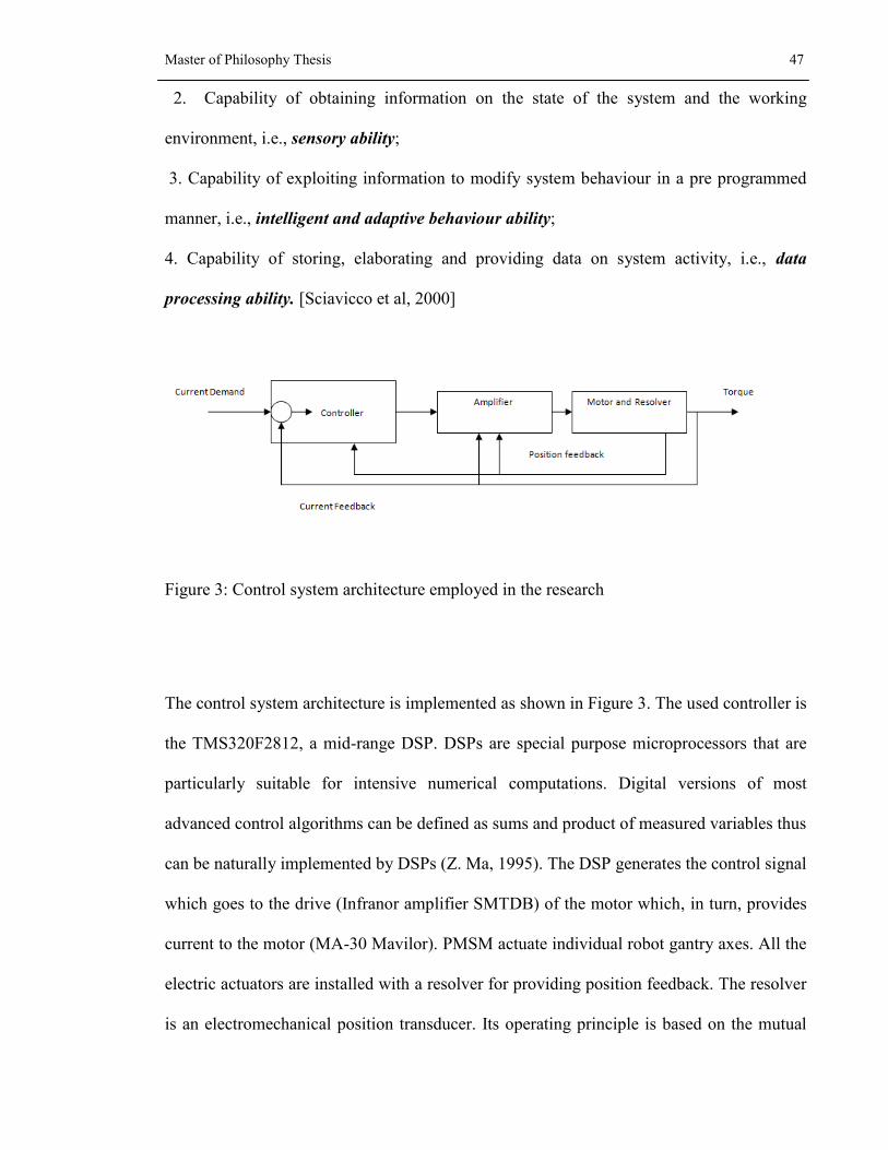
Figure 3: Control system architecture employed in the research

The control system architecture is implemented as shown in Figure 3. The used controller is

the TMS320F2812, a mid-range DSP. DSPs are special purpose microprocessors that are

particularly suitable for intensive numerical computations. Digital versions of most

advanced control algorithms can be defined as sums and product of measured variables thus

can be naturally implemented by DSPs (Z. Ma, 1995). The DSP generates the control signal

which goes to the drive (Infranor amplifier SMTDB) of the motor which, in turn, provides

current to the motor (MA-30 Mavilor). PMSM actuate individual robot gantry axes. All the

electric actuators are installed with a resolver for providing position feedback. The resolver

is an electromechanical position transducer. Its operating principle is based on the mutual


induction between two electric circuits which allow continuous transmission of angular

position without mechanical limits.

Each motor is connected with two cables. One cable carries electric power to the motor.

The second cable (resolver cable) tells the amplifier cabinet how far the motor has moved

in a positive or negative direction. The motor and amplifier form a separate unit. There is a

current feedback path from the motor and a position feedback path from the resolver on the

motor, as shown in Figure 3. The data sheets for the electric actuator, amplifier and

controller can be found in the appendix I, II and III.

As the research work is performed on a two dimensional gantry manipulator, there are two

DSP boards used in the architecture. The two DSP boards communicate with each other via

a CAN bus interface with a maximum speed of 1Mbps. The experimental setup has been

designed for X-Y two dimensional tasks at present, but it has also a

facility for a Z direction.

Figure 4: Block diagram of Vector control of an AC motor

(Detailed Description of Vector Control is given in the Appendix section-05)


The electric actuators on the robot are operated by Vector control. It is an elegant method

of controlling the PMSM which is used to control space vectors of magnetic flux, current,

and voltage. It is possible to set up the co-ordinate system to decompose the vectors into an

electro-magnetic field generating and torque generating parts. Thus, the structure of the

motor controller (vector control controller) is almost the same as for a separately excited

DC motor, which simplifies the control of PMSM. This vector control technique was

developed in the past especially to achieve similar excellent dynamic performance of

PMSM.

The performance of three phase ac machines is described by voltage equations and

inductances. AC machine inductances are functions of rotor speed. The coefficients of the

differential equations which describe the behaviour of these machines is time varying. A

change of variable can reduce the complexity of these differential equations. Therefore,

Clarke and Park Transforms were introduced. The transformation of rotational circuits to a

stationary circuit was developed by E. Clarke. The Park Transform was developed by R. H.

Park. The Park Transform has the feature of eliminating all time varying inductances from

the voltage equations [Toliyat, 2004]. Using these transforms, many properties of the

electrical machines can be studied without the complexities of the voltage equations.

Vector control seeks to recreate the orthogonal components in the AC machine (id and iq)

in order to control the torque producing current separately from the magnetic flux

producing current [Vector Control, NEC, 2002]. The iq and id components of the

(fictitious) stator current vector are referenced to the so-called rotor reference frame. This


reference frame is referenced to the rotor flux, and is synchronous to the rotor. There may

be a phase difference, but this is usually assumed to be zero for our discussion. The axis

along the rotor flux is the d (or direct) axis, and the axis 90 degrees (electrical) away from it

is the quadrature (q) axis. Theta is the rotor flux position.

In a PMSM the flux component is produced by the permanent magnets (the fixed field

winding is replaced with a rotating permanent magnet). The rotor flux produced by the PM

rotates at the same speed as the rotor field i.e. there is no slip. So for a PMSM the ordered

dI component is set to zero and the rotor angle is obtained by integrating the rotor speed.

The system configuration for vector control of a PMSM. For all the following transform

equations, refer to Figure 4.

Vector control requires computationally intensive algorithms, this coupled with closed loop

control and precise Pulse Width Modulation (PWM), requires a relatively powerful

microprocessor along with the relevant peripherals to make vector control a practical

proposition. This Vector control is implemented inside the amplifier. Although this can also

be implemented in software, as the DSP controller has a very high sampling frequency.

4.3 Data acquisition, interpretation and utilisation in the controller

Signal conditioning means manipulating an analogue signal in such a way that it meets the

requirements of the next stage for further processing. More generally, signal conditioning

can include amplification, filtering, converting, and any other processes required to make

sensor output suitable for conversion to digital format. It is primarily used for data

acquisition, in which sensor signals must be interpreted and filtered to levels suitable for


Analogue-to-Digital Conversion (ADC) or Digital-to-Analog Conversion (DAC) so they

can be read by computerized devices.

The F2812DSP accepts analogue signals which are 0-3.3V. All the feedback signals from

the amplifier are 0-10V. So, signal conditioning boards were manufactured to level shift

these to input them into the DSP. The current signal from the amplifier is an analogue

signal and has to be digitised which is done by the 12 bit ADC on board of the F2812 DSP

with a fast conversion rate of 80ns at 25 MHz clock. Also, the output speed command from

the DSP has to be in the range of 0-10V as the amplifier accepts 0-10V analogue signal at

its input. There is also a DAC to convert it into an analogue signal. The other DSP

functionalities used is the Serial Peripheral Interface (SPI), which is used for

communications between the DSP and external peripherals or controllers. The SPI is a

high-speed synchronous serial input/output (I/O) port that allows a serial bit stream of

programmed length (one to sixteen bits) to be shifted into and out of the device at a

programmed bit-transfer rate. The circuit diagrams for the signal conditioning boards are

included in the appendix of this thesis.

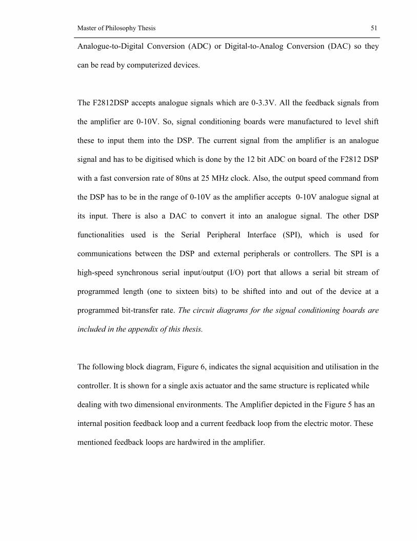
The following block diagram, Figure 6, indicates the signal acquisition and utilisation in the

controller. It is shown for a single axis actuator and the same structure is replicated while

dealing with two dimensional environments. The Amplifier depicted in the Figure 5 has an

internal position feedback loop and a current feedback loop from the electric motor. These

mentioned feedback loops are hardwired in the amplifier.


The 2812 DSP position feedback loop and current feedback loop are depicted in grey boxes

are designed in the software. These 2812 DSP feedback loops are separate to the amplifier

feedback loops. Due to the hardwired feedback loops in the amplifier, the research work is

focused only on the feedback loops in the 2812 DSP.

The Figures 6, 7 and 8 show the experimental setup used in the research.


Figure 5: Block diagram of the control system architecture implemented for a single robot axis

(Same architecture is employed when used for 2 dimensional environments)

TMS320F2812 D.S.P.

board Spectrum Digital

board

Digital to

analog

converter

Signal from the

S.P.I

Amplifier

0-10V

signal

0-3.3V

signal

Motor (P.M.S.M.)

Resolver

Ia, Ib Ic

Currents

Position

feedback

Current feedback

from the motor

Signal conditioning board 1

Signal conditioning board 2

θposition

(0-5V)

I current

(0-10V)

Current feedback into

the DSP board (0-3V)

Position

feedback

(0-3.3V)

Input

signal into

Ato D of

the DSP


Figure 6: Robot manipulator Figure 7: Two arms of InFACT

Figure 8: robot electric actuator and manipulator


4.4 Calibration of motor current to force experiment

When the robot interacts with an environment there is a change in the level of current in

the electric actuator because the load torque increases. The motor current which reflects

the torque, is calibrated to reflect the force exerted on the environment. The robot

manipulator is made to interact with the environment, as shown in Figure9, and the current

from the electric actuator is monitored. As shown in the Figure 9, the end effector is in

contact with the metal surface. The torque command is then increased which results in the

level of current. Therefore, the force exerted by the robot manipulator increased. This

force exerted by the manipulator is recorded using a spring balance connected between at

the tip of the end effector.

The experiment was conducted for different commanded torque values and the

corresponding force is observed in the spring balance. In Figure 10, the calibration

experiment is conducted to obtain a relationship between the electric motor current to

force.As shown in Figure 10, the force and current graph is plotted. It is found out that the

force exerted bears a two-part linear relationship to the current of the motor, shown in

Figure 10. This relationship is used in the software for control structure purposes. The two

linear regions can be seen in the Figure 11 and this characteristic is incorporated in the

software. The experimental work in the Thesis was carried out in the first linear region of

the graph as shown in Figure 11.


Figure 9: robot interaction with environment (a metal artefact)

Figure 10: Calibration of the motor current to force


Figure 11: Calibration of the electric motor current to force with two linear regions

4.5 Development of the system and initial robot interaction experiments

After the force-current calibration experiment on the robot manipulator was conducted,

the robot was made to interact with the environment with different torque limiting values.

As seen from the Figure 13, the robot interaction was controlled with pre-specified values.

This shows that the torque from the electric actuator can be made programmable in real

time and the interaction can be controlled accurately and precisely in the software.


Figure 12: Graph showing torque/current limiting values over 10 seconds interval.

The Y axis is the scope readings from 0 to 10 seconds. The Figure 12 shows the three

stages of the robot interaction with the environment. The Part A is the robot approach

towards the environment. The Part B is the actual interaction with the environment and

afterwards it settles down after the step change. The Part C is the increase of the force

level on the environment to predetermined values which is termed as the current limiting

values. The entire event is monitored on an oscilloscope.


4.6 Approach to development of contour following system

The research is based on the electric actuator force control on unknown geometrical

environments. Therefore, a 2D contour following system was created. The contour

following task is one of the most common control problems encountered by

servomechanisms such as X-Y tables, robot manipulators and CNC machine tools [Cheng,

2005, Chen, 2000]. In this research work, two processors are used for each individual axis.

In the following equations, nf is the normal force while tf is the tangential force applied

on the surface. The resultant force is f as shown in Figure 13. While following two

dimensional contours, the resultant force f is kept within the tolerance band set by the

controller. This resultant force can be altered depending on the geometrical surfaces

encountered during a control following system.

Figure 13: The force vector components nf & ft and the resultant force vector tf

Experiments were planned on the robot manipulator for following surfaces with unknown

geometry. The Figure 14 shows the various surfaces used in the experiments. In these


experiments only the start and the end points of the surface where input into the controller.

The tests and results from these surfaces are in the next chapter.

Figure 14: Different geometric surfaces used for 2 dimensional contour following with the

knowledge of starting (A) and finish (B) points

4.7 Software development flow charts

A real time system is defined, according to Oxford dictionary, as “any system in which the

time at which the output is produced is significant”. This is because the input corresponds


to some movement in the physical world, and the output has to relate to that same

movement. Another way of thinking about real time systems is any information

processing activity or system which has to respond to externally generated input stimuli

within a finite and specific period.

Algorithm development is very crucial phase during software concept and specification

phase of a real-time system. This section shows the software development of a basic two

dimensional system which was used for robot contour-following with unknown geometry.

It describes the development of the software rationale with the aid of flow charts. The

software architecture was designed on a single axis and then both the axes were

incorporated. Further investigations led to the inclusion of PID control and Fuzzy control

in the software and that has been described in the subsequent chapters of this thesis. The

software was written in the C language on the F2812DSP (Texas Instruments Code

Composer Studio®). The entire software code is included in the appendix of this thesis.

The following flowcharts describe the basic development of the software in three stages:

1. Single axis robot interaction with the environment with force control loops, Figure 15.

2. Two axis robot interaction with the environment with one axis performing force loop

while the other position loop operation, Figure 16.

3. Two axis robot interaction with the environment with the inclusion of both force control

and position control loops, Figure 17.


Figure 15: Flowchart describing robot electric actuator with the environment

The flow chart describes the algorithm for a single axis electric actuator. The robot

initializes itself in a speed/position loop until it detects any external environment. If it

does not encounter any external environment it remains in speed loop. However, on


encountering the environment it enters into a force control loop and exerts the desired

force, which is real time programmable and is within certain predetermined tolerance

limits.



dimensional surfaces

The first flowchart has been modified to include a two dimensional environment. The

communication between the controllers is achieved through a Controller Area Network

(CAN). The controllers are termed as X and Y representing the 2D environments. The X

controller is initialized in the speed/position control loop until an environment is detected.

When the X controller enters the force control loop, it initializes the Y controller through

the CAN to start traversing the environment. So the robot manipulator can be used to deal

with 2D environments. In this software structure, the Y controller always stays in the

position loop whilst the X controller stays in force controlled loop. The control algorithm

can perform for a basic 2D contour following environment whilst exerting a constant

desired force.

The third development is as shown in Figure 18. The X axis starts first in speed control

until it interacts with the environment. As soon as the X controller detects any external

environment, it switches to current control and thereby force/ torque control. As it exerts

the desired force on the environment, a CAN signal is issued to the Y controller to start

motion across the traverse of the environment. The Y axis controller now detects any

increase in the feedback current. If there is an increase in the current, it asks the X

controller through the CAN to switch into speed control and reverse back, while the Y

controller exerts force on the environment. This is done according to the resultant force


vector between the X and Y axes force individual components. The X and Y axes

controllers have position and force loops intertwined together and are switched depending

on the circumstances. The Y axis controller always checks for a desired position signal. It

issues a stop signal as soon as it encounters the desired position and forwards this

information to X controller, which also stops. Otherwise, both the controllers stay in their

respective loops. As the DSP controllers are very fast, the software has to be slowed down

to match with the amplifier of the motor. Otherwise, the DSP issues commands which the

amplifier cannot execute and results in an unsteady, jerky behaviour of the manipulator.



dimensional surfaces


Chapter 5

5. PID control modelling and implementation on the experimental system

5.1 Background and Introduction

Control systems engineering is a fascinating and important field. A control system is a

device or set of devices to manage, command, direct or regulate the behavior of other

devices or systems. It encompasses the methods and techniques for a continuous

monitoring of the operating state of the system without operator intervention. These are

referred as closed loop control systems which have the ability of automatically correcting

its own behaviour so the desired results/outcomes are reached. Control engineers often

utilize system/plant feedback to design control systems. For example, in an automobile

with cruise control the vehicle's speed is continuously monitored and fed back to the

system which adjusts the motor's torque accordingly.


Figure 18: Block representation of a process with input output variables

As an example, as shown in Figure 18, the process is a physical system to be controlled.

The control variable or the manipulating variable is the parameter which the controller

uses to control or manipulate the process. The process output variable is the variable to be

controlled so that it becomes sufficiently close to the set point. The disturbance is a non-

controlled input variable to the process which affects the process output variable. The aim

of the control algorithm is to adjust the control variable so that the control error

(difference between the set point and the process output variable) is within

acceptable/desired limits [Haugen, 2004].

As an example, in 1788, James Watt constructed a speed control system for a steam

engine. Watt’s speed control was based on feedback from measured rotational speed to the

opening of the steam valve via a centrifugal controller which was based on a simple

principle. The larger the speed, the smaller the valve opening (and steam supply), and vice

versa acting proportional to the error. In this way the speed was held at or near a constant

set-point value, despite the disturbances as variations in the steam pressure and changing


load torques acting on engine shaft. Watt’s speed control system is regarded as the first

industrial application of control engineering. It was based on experiments and trial and

error. In 1868, James C. Maxwell made a mathematical analysis of the speed control

system, and this analysis may be regarded as the starting point of the theoretical methods

for analysis and design of control systems. [Haugen, 2004]

5.2 Introduction

Motion control deals with the use of high performance electric motors and is a very

important part of industrial control systems. Motion control includes applications for

speed and torque or position control in practically all branches of industry. Sophisticated

motion control systems bring greater accuracy, flexibility and parameter sensitivity to the

applications [Lorenz, 1994, Kiel et al, 1995, Bose, 1994]. As a consequence of this

progress, more and more applications that have used simple electric drives for economic

reasons are being replaced by motion control systems [Texas Instruments website, 2008].

The motion controller of the electric actuator (PMSM), used in the research, requires

position feedback for electronic commutation. As the aim of the research is to perform

torque control in the electric motor for controlled interaction with the environment, the

controller also uses the current feedback from the motor. The current (calibrated to force)

is compared with the desired force required and the controller takes appropriate action to

equalise the current and desired force values. The research is focussed on the interaction


of the robot end effector with an unknown environment. Therefore, due to these process

nonlinearities, closed loop control is required for the interaction forces to be regulated

within the desired force tolerances.

This is commonly applied by a PID controller. It has enjoyed popularity as a purely

mechanical device and as an electronic device. [Wescott, 2008]. A PID controller is a

generic control loop feedback mechanism widely used in industrial control systems for

over 50 years. A PID controller attempts to correct the error between a measured process

variable and a desired set point by calculating and then outputting a corrective action that

can adjust the process accordingly. It is a robust easily understood algorithm that can

provide excellent control performance [Willis, 2008, PID website, 2008, Bhattacharya,

2004]. The PID algorithm consists of three basic modes, the Proportional mode, the

Integral and the Derivative modes. When utilising this algorithm it is necessary to decide

which modes are to be used and then specify the parameters (or settings) for each mode

used. Generally, three basic algorithms are used P, PI or PID. The controllers are mainly

used to reduce the fluctuations and also to minimize the error.

The ideal PID controller is in the following form:

t

dp

i

p

pdt

deTKed

T

KeKuu

00 ......................................................... (21)


In equation (21), there are three parameters. Kp is the Proportional gain, Td is the

Derivative time, e is the control error, u is the control variable and ou is the nominal

control variable.

P-Controller

The P controller calculates the control variable according to puuu 0 as follows:

eKuu p 0 ................................................................................................................... (22)

and up= Kpe

where up is the P-term [6]. The operation of the P-controller is to adjust the signal control

accordingly or proportional to the error. By increasing the Kp value the static control error

can be minimised in the controller as it gives more control to the variable adjustment Kpe,

when the Kp value is increased for a give error e. This produces a small error. The

limitation of this controller is that while the value of Kp is increased there is a reduced

stability for the control loop and also when this value is increased by a large magnitude,

the control loop becomes unstable [Haugen, 2004].

PI-Controller

In the PI controller (proportional + integral) the control variable is calculated as


deT

KeKuu

t

i

p

p 0

0 ................................................................................ (23)

and deT

Ku

t

i

p

i 0

Here, ui is the integral term, Kp is the proportional gain. Ti (s) is the integral time. Ki is the

integral gain. The integral term is very essential and is calculated continuously from the

initial time when t=0 to the present point of time. This is the known as the integral of the

control error. The contribution from the integral term is proportional to both the

magnitude of the error and the duration of the error. Summing the instantaneous error over

time (integrating the error) gives the accumulated offset that should have been corrected

previously. The accumulated error is then multiplied by the integral gain and added to the

controller output. The integral term (when added to the proportional term) accelerates the

movement of the process towards set-point and eliminates the residual steady-state error

that occurs with a proportional only controller. However, since the integral term is

responding to accumulated errors from the past, it can cause the present value to overshoot

the set-point value (cross over the set-point and then create a deviation in the other

direction).

PID-Controller

This is a faster controller than the PI controller due to the addition of a control variable

which is proportional to the time derivative or the rate of change of error e.


t

dp

i

p

pdt

deTKed

T

KeKuu

00 ............................................................. (24)

where dt

deTKu dpd this is the derivative term.

In derivative controller, the rate of change of the process error is calculated by

determining the slope of the error over time (i.e. its first derivative with respect to time)

and multiplying this rate of change by the derivative gain. Thus, the PID controller can

adjust process inputs based on the history and rate of change of the error signal, which

gives more accurate and stable control. It can be shown mathematically that a PID loop

will produce accurate stable control in cases where other control algorithms would either

have a steady-state error or would cause the process to oscillate [PID website, 2008].

A conventional PID controller is depicted in Figure 19.

Figure 19 - A Traditional PID Controller


The controller sensor senses the signal, compares it with the setpoint value and determines

the error. This error is then used to compute the change needed in input so as to eliminate

the error from the output of the process. Thus in the PID loop, the function of the

Proportional is to terminate the error present in the process at that point; the function of

the Integral is to calculate the time for which the error has not become acceptable and the

function of the Derivative is to estimate possible future error according to the rate of

change of the past error.

5.3 Approach to the development of the PID controller

The gains of the PID controller need to be accurately tuned to achieve the desired results

from the controller. The performance of the controller is often related to “fast control but

with satisfactory stability” [Haugen, 2004]. There are various methods of tuning the actual

PID gain parameters. They are based on trial and error methods, Zeigler Nichols method

or the tuning software packages.

In this research work, the electric actuator is driven by an amplifier. As the electric motor

is PMSM, it requires position feedback for commutation purposes. Therefore, the

amplifier has a built in PID controller for the internal loop which facilitates the

commutation. The PID controller designed and presented, in this chapter, is for the closed

loop of the torque control in the system. The open loop response of the plant was observed

and depending on that the PID controller is designed. PID controller is used in the


research work because of the intrinsic qualities simplicity in implementation and

reliability in the motion control systems [Haugen, 2004].

5.4 Modelling and validation of the controller

The modelling of the PID controller is done in MATLAB/Simulink and then the PID

controller is implemented on the experimental set-up for contour following experiments.

The step input to the plant was a speed command and the current from the motor was

observed for an open loop system. An overshoot in the response of the system was

observed. From these tests on the experimental setup, the damping ratio and the natural

frequency of the system were calculated and a second order transform function was

obtained. It was modelled in MATLAB Simulink and a PID controller was developed

using trial and error method as shown in Figure 22. This was then tested on the

experimental setup by providing a step input to the system. As seen in Figure 24, the

overshoot was reduced with the inclusion of the PID controller. The PID controller is

designed based upon this criterion.

The calculation of the transfer function from the system/plant response to step inputs was

carried out. The damping ratio and the natural frequency were observed for a number of

trails as shown in Figures 20 and 21 . The damping ratio is calculated by measuring the

amount of damping present in a system in the rate of decay of free oscillations.

Logarithmic decrement can be defined as the natural logarithm of the ration of any two

successive amplitudes. It is defined as follows:

δ = ς ωn τ ≅ 2πς


Figure 20: Different values of ζ calculated from the step inputs to the plant

Figure 21: Different values of ω n calculated from step inputs to the plant

The calculation of the transfer function is carried out by damping ratio and natural

frequency of the system by observing the open loop response of the system.

ζ= 0.75, 0.74, 0.64, 0.66, 0.59, 0.66

n = 2.96, 1.98, 1.75, 2.69, 1.6, 2.45

Transfer function= n

2/ s

2 +2 ζ n s + n 2


= 4.97/ s2+ 2.98 s+ 4.97

Figure 22– Simulink model for the PID controller implementation and comparison with

plant open loop response. (Kp=1.4, Ki=2.8, Kd=0.18)


Figure 23 - Graph showing the Simulink plant output with and without PID control

The graph, in Figure 23, was obtained whilst following a straight surface. The first section

is approaching the surface. As the robot interacts with the environment, there is a step

change and it exerts a constant force as it follows the surface. An experimentally tuned

PID controller is implemented in the software. In the open loop output response of the

plant, there was a small overshoot which was eliminated with the PID controller. The

values of PID are different in the model and the plant because the real plant has some

amount of energy loses which are neglected in the simulation studies.


Figure 24 – Practical implementation of the PID controller on the Experimental

setup(Kp=0.001, Ki=0.002, Kd=0.01)

5.5 Results and Conclusion

Experiments are performed, using the PID controller, on the practical setup for contour

following experiments with unknown geometry. The robot gantry manipulator was

allowed to interact with different metal surfaces with varied geometries. The resultant

force acting on the surfaces was monitored and the results are as shown in Figures 25 and

26. The feedback current values, calibrated to force (Newtons), are presented in the

graphs. It is observed that the force values remain in the desired force band with an error

of 2N. A B

Figure 25: Force profile while following a straight surface


Figure 26: Force profile following an inclined surface

5.6 Further Development with PID Controller

The PID controller, employed in the research, has fixed gains. However, PID controller

gains might need to be retuned whenever the processes are subjected to some kind of

disturbance or when processes present complexities and nonlinearities. The controlled

interaction of the robot force control with surfaces of different geometries suffers from the

problem. Over the last few years, significant development has been established in the

process control area to adjust the PID controller parameters in an automatic way, in order

to ensure desired behaviour for a closed-loop plant. [Astrom &Wittenmark, 1989; Coelho

et al., 1998; Coelho & Coelho, 1998; VanDoren, 1998]. This aspect can be further

enhanced by using gain scheduling or the self-tuning of these gains which has been


demonstrated in these researches [Kazemian, 2001, Huang at al, 1996, Wang et al, 1998].

The self-tuning PID controllers can be designed using Fuzzy logic and neural networks in

multivariate nonlinear environments. In [Malki et al, 1997], a fuzzy PID control is

designed for flexible joint robot arm with uncertainties from time varying loads.


Chapter 6

6. Development and Implementation of Fuzzy Logic

Controller on the experimental system

6.1 Introduction and Justification for the need of fuzzy controller.

The previous chapter was based on the torque control of the robot electric actuator using

PID control. The work proved that the interaction of the robot interaction was

experimentally force controlled for surface following applications, without previous

geometrical knowledge. The results of the PID control algorithm are in the range of ±2N

based on the present experimental setup.

The application of PID controller is widely used in single loop controllers, distributed

controllers and Programmable logic controllers and the performance is satisfactory in

simple applications [Juang, 2008, Lyguoras, 2007]. The presented research work is

focused on automation of manufacturing techniques such as deburring and polishing


which deal with complex, nonlinear and noisy environments. Therefore there is a need to

have an adaptive controller which deals with these complexities. Fuzzy logic, which

simulates human thinking using linguistic variables, can be applied as it takes into account

the imprecision inherent in physical systems. Therefore, with the aim to accommodate

complex environments and thereby the nonlinearities in them, fuzzy logic is introduced in

the software to accommodate these conditions.

The concept of Fuzzy Logic (FL) was conceived by Lotfi A. Zadeh, professor at the

University of California at Berkley. Professor Zadeh reasoned that people do not require

precise, numerical information input, and yet they are capable of highly adaptive control.

If feedback controllers could be programmed to accept noisy, imprecise input, they would

be much more effective and perhaps easier to implement. Therefore, FL is a problem-

solving control system methodology that lends itself to implementation in systems ranging

from simple, small, embedded micro-controllers to large, networked, multi-channel PC or

workstation-based data acquisition and control systems. It can be implemented in

hardware, software, or a combination of both. FL provides a simple way to arrive at a

definite conclusion based upon vague, ambiguous, imprecise, noisy, or missing input

information [Seattle Robotics].

Conventional control systems use the physical models to deal with the process. That is

time-consuming and needs a theoretical background of the designer. But many processes

can be controlled by human being without any model, and these processes cannot be


controlled by conventional control systems. At first fuzzy control was treated with

mistrust by the engineers who started with the conventional control theory. When fuzzy

control systems were widely used in manufacture in Japan, people began to know fuzzy

control system are cheap, easy to design, very robust, and better than the conventional

control system.

6.2 Approach adopted in designing the fuzzy controller

Fuzzy controllers are special modern computer-controlled systems that use the rules to

model process knowledge. The designer use rules to link the input variables with the

control variables by linguistic variables. Human beings make decisions based on rules.

Even though, we may not be aware of it, all the decisions we make are based on computer

like if-then statements. Rules associate ideas and relate one event to another. Fuzzy

machines, which always tend to mimic the behaviour of man, work the same way. Only

this time the decision and the means of choosing that decision are replaced by fuzzy sets

and the rules are replaced by fuzzy rules. Fuzzy rules also operate using a series of if-then

statements. For instance,

if <conditions, and if satisfied>, then <action>

For example, if<force exerted on the environment is more than desired force>,

then<reduce the current and thereby torque of the motor>

Linguistic rules describing the control system consist of two parts; an antecedent block

(between the IF and THEN) and a consequent block (following THEN). Depending on the


system, it may not be necessary to evaluate every possible input combination since some

may rarely or never occur. By making this type of evaluation, usually done by an

experienced operator, fewer rules can be evaluated, thus simplifying the processing logic

and perhaps even improving the FL system performance.

Figure 27: Example of membership functions[Mathworks website]

Figure 28: Fuzzy logic membership functions example[Mathworks website]


As shown in Figure 28, the membership function is a graphical representation of the

magnitude of participation of each input. It associates a weighting with each of the inputs

that are processed, define functional overlap between inputs, and ultimately determines an

output response. The rules use the input membership values as weighting factors to

determine their influence on the fuzzy output sets of the final output conclusion. The

triangular shape is common, but bell, trapezoidal and, exponential have been used. More

complex functions are possible but require greater computing overhead to implement.

Once the functions are inferred, scaled, and combined, they are defuzzified into a crisp

output which drives the system. There are different membership functions associated with

each input and output response. As shown in Figure 29, an example is given for error and

error dot triangular membership functions. The error is the difference between

current/present value and the desired value. The error dot is the rate of change of this error

with respect to time.

Mamdani fuzzy inference method is the most commonly seen fuzzy methodology.

Mamdani method was among the first control systems built using fuzzy set theory. It was

proposed in 1975 by Ebrahim Mamdani as an attempt to control a steam engine and boiler

combination by synthesizing a set of linguistic control rules obtained from experienced

human operators. Mamdani effort was based on Lotfi Zadeh's 1973 paper on fuzzy

algorithms for complex systems and decision processes. Fuzzy control, which directly

uses fuzzy rules, is the most important application in fuzzy theory.


The following are the basic steps in the implementation of a Mamdani fuzzy controller:

1. Input: number of input signals, number of derived states of each input signal,

scaling

2. Fuzzification: type of membership functions, number of membership functions

3. Rules: number of antecedents, structure of rule base, type of membership

functions in consequences.

4. Rules evaluation: aggregation operator in the antecedent

5. Aggregation: aggregation operator combining the results of individual rules

6. Defuzzification: defuzzification procedure

7. Output: number of output signals, scaling.

Mamdani fuzzy logic controller is used when the control problems require low accuracy

and trivial minimal performance. The second widely used fuzzy controller is the Tagaki-

Sugeno fuzzy controller. It represents an effective representation of complex non linear

systems in terms of fuzzy sets and fuzzy reasoning and is demonstrated in these research

works [Ying, 1999, Garcia-Perez,1996, and Shih,1992]. Takagi-Sugeno fuzzy logic or

Sugeno fuzzy logic was first introduced in 1985. It is the modification of Mamdani fuzzy

logic. Fuzzifying the inputs and applying the fuzzy operation are exactly the same of

Mamdani fuzzy logic. The different place between them is the output membership

function. Sugeno-type’s output membership functions are only linear or constant. When

the output functions are constant, it can be called as zero-order Sugeno fuzzy model. For

example, we can define a zero-order Sugeno fuzzy logic as:


If x is A and y is B, then z = k.

Where A and B are fuzzy set defined for the membership functions for x and y. k is a

constant crisp value defined in the consequent. So the output of each rule is like a spike.

The operator of implication and aggregation methods is simply multiplication and

addition.

The first-order Sugeno fuzzy logic model has the rules like that:

If x is A and y is B, then z = p * x + q * y + r.

Where A and B are fuzzy sets in the antecedent, while p, q and r are all the constants.

A Sugeno fuzzy inference system is extremely well suited to the task of smoothly

interpolating the linear gains that would be applied across the input space; it is a natural

and efficient gain scheduler. Similarly, a Sugeno system is suited for modeling nonlinear

systems by interpolating between multiple linear models. The advantages of Tagaki

Sugeno Fuzzy logic controller are suitable to compute, can optimise the parameter to

improve efficiency and uses linear techniques to control non linear environments. The

disadvantage is that it is not an intuitive controller and becomes complex as the order

increases [Seattle Robotics website, Mathworks website].

Because it is a more compact and computationally efficient representation than a

Mamdani system, the Sugeno system lends itself to the use of adaptive techniques for


constructing fuzzy models. These adaptive techniques can be used to customize the

membership functions so that the fuzzy system best models the data.

6.3 Implementation and Tests

The fuzzy logic control designed for the research is the Tagaki Sugeno fuzzy logic. The

basic aim was to design a controller for dealing with complex environments. The robot

force interaction with the environment is a complex multi input multi output (MIMO)

system and the controller has to accommodate changes related to unpredictability of the

environment, noise from the experimental setup, marginally stable processes and time

varying process [Bhattachatya, 2003, Li 1998].

Precision deburring and polishing is mostly done by skilled human operators which are

familiar with the process. When they grind a large burr they do not remove the large burr

all at once but they usually move the tool back and forth so that the burr can be removed

in an optimal manner. They may also accommodate the force applied to the tool in order

to touch the burr gently without any damage to the tool or the work piece. Thus the

operators monitor the state of the given task process and take control actions. The control

behaviour of human experts can be represented in an IF-THEN relationship as used in

fuzzy logic.

The expertise of an operator is difficult to describe in an analytical way. The task executed

by the human operator has no detailed algorithms or methodology (Aertbelien et al, Asada


et al). The fuzzy control can be designed based on the human characteristics used in

surface following operations. The stiffness of the electric actuator can be made

programmable.

Therefore for following two dimensional surfaces with unknown geometry three input

variables in the fuzzy logic scheme are used. They are explained as follows:

1. The first is the error (e), which is the difference between the desired and actual force

acting on the surface. This is for ensuring the current of the motor remains in the required

desired band.

2. The second is the change of error (Δe), which gives the rate of change of error as the

contour is being followed. The change of error term is crucial in the controller structure as

it depicts the contour being followed.

3. And the third is the speed of traverse across the surface (v), which is the tangential

velocity of the tool across the surface. The speed of the traverse of the tool is important as

it affects the finishing in the deburring process and affects the tracing of geometrical

profiles in surface following operations.


Figure 30: Design of Tagaki Sugeno fuzzy logic controller and specifying inputs and

outputs

The fuzzy logic controller has been implemented in the software. The following Figures

31 and 32 show the resultant force profiles whilst following straight and inclined surfaces.

In Figure 31, the surface is between the points A and B. It is seen that that the force is

within the desired tolerance band. It has been seen that the force remains within the user

desired force tolerance range.

Figure 31: Force signature while following an inclined surface using fuzzy logic


Figure 32: Force signature while following an inclined surface using fuzzy logic

6.4 Comparison between the performance of PID and fuzzy controllers

The following table depicts the comparison between the PID and the fuzzy control

implemented on the experimental rig.

1. The comparison between the PID and fuzzy controller is based firstly on the speed

of execution of the software. This factor decides the responsiveness of the system.

The execution speed of the fuzzy control is large than that of PID controller.

Therefore, the fuzzy control can be implemented in cases where it is needed only


and thus the computational time is saved and the responsiveness of the controller

to any change can be improved.

2. The second comparison is based on the force deviation range whilst following

contours with unknown geometries. While following simple geometrical shapes

without any complexities, the force error band is ±2N in case of PID controller

while it is±1N in case of a fuzzy controller.

It is noted that the performance of these controllers is affected by the performance

of the drive amplifier of the electric motor. The drive amplifier, in the present

experimental setup, due to its lower speed reduces the system responsiveness and

thereby the performance of the system. Secondly, the presented experimental work

is carried out on a robot gantry manipulator with multiple degrees of freedom. The

joints which are not used in the experiments are mechanically clamped. It is

observed while performing the experiments that there is some introduction of a

mechanical compliance and thereby it affects the performance.

The research work done with an aim to demonstrate a generic control philosophy

of torque control in electric actuators. As stated earlier, this work is suitable to

generalisation and this adaptive control structure can also be applied.



3. While following simple geometrical shapes with some nonlinear complexities, the

force error band is ±2N in case of PID controller while it is±1N in case of a fuzzy

controller. But it is observed that whilst reproducing the geometrical profile of the

surface, the fuzzy controller is smoother rather than the jerky behaviour of the PID

controller.



4. The overshoot from the PID controller is 0.33% of the F.S.V. (Full Scale Value)

and from the fuzzy controller is 0.2% of FSV.

Execution speed

(µs)

(Software based)

Force error

(N)

Simple shapes

Force error

Complex shapes

(N)

Overshoot

PID

Controller

3.62 µs ±2N ±2N 0.33% of FSV

Fuzzy Controller 12.8 µs ±1N ±1N 0.2% of FSV


Table 35: Performance comparison between PID and Fuzzy Controller on the

experimental rig

6.5 Proposed modified controller structure for PID+Fuzzy Controller

The torque control in electric actuator for the robot interaction with the environment has

been demonstrated with the PID controller and the fuzzy controller. The PID controller

due it its ease of implementation and good performance can be used for simple control

tasks while the fuzzy controller can be incorporated whilst dealing with complex non

linear environments. Therefore, in this section a modified control strategy has been

proposed to include both the PID and the fuzzy controllers in a single control structure and

to have a switching mechanism between the two controllers based on a selection criterion.

As shown in the following block diagram, Figure 37, the decision for the controller is

based on selection criterion and the decision is made in real time. The torque and position

of the motor are monitored in real time and the force error and rate of change of force

error information is used for the selection criterion. For example, in deburring or surface

following operations, when the surface geometry is simple, PID controller is implemented

when the error and change of force error are within the acceptable band. If the surface

geometry changes, it is indicated in the error and rate of change of error, fuzzy logic is

introduced to deal with complex non-linear environments. The transition from one

controller to the other is done gradually so there is no jerky behaviour in the system which

is important for surface finishing operations such as deburring.


Figure 36: Modified Controller structure for PID+Fuzzy controllers


Figure 37: Profile of the surface following using the modified control strategy


Chapter 7

7. Main Contributions and Conclusions of the research

This work presents an approach for the control of robot electric actuators when the robot

interacts with an external object or surface. The presented research work is primarily

based on achieving accurate torque control in the robot electric actuators and introduction

of software compliance in the system. The controlled interaction results in a stable and

specified force contact with the surface. Therefore, robot force control is accomplished

without the inclusion of any external sensors in the system. The subordinate advantages

are cost, adaptable to different working conditions and increase in the responsiveness of

the system. Due to these mentioned advantages, the control philosophy can be adapted to

the traditionally manual manufacturing techniques such as deburring, composite layouts

and also can be used in coordinate measuring machines.

The following are the main contributions of the presented work:

1. Introduction of compliant behaviour in electric actuators


A broad literature survey was carried out for robot force control. It was concluded

that the current robot force control strategies employed for the interaction with the

environment or object have inherent stiffness and rely on the sensory feedback to

realise interaction forces. The research work has demonstrated the compliant

behaviour, by varying the stiffness, in the joint robot electric actuators. The control

philosophy, as opposite to stiff surfaces is applied in real time where the robot

interacts with an external environment. This is achieved in real time torque control

in the robot electric actuators. There are no external sensors connected to the robot

and this was demonstrated on the experimental setup. The research has shown that

the electric actuator stiffness can be altered and it can be compared to be a

programmable spring.

2. Mathematical representation of PMSM for torque control

A mathematical representation of the electric actuator (PMSM), used in the

research, is carried out. The operation of PMSM requires Vector control includes

the decomposition of the three stator currents into imaginary two axes components

for simplification of the operation. The derivation of torque to current and thereby

relating it to the force exerted on the system. The operation of PMSM is difficult

and the control philosophy has been demonstrated on the same platform and

therefore, the presented research work presented is suitable for generalisation to

other electric actuators such as dc motors.


3. Application for contour-following systems without geometrical knowledge

A two dimensional contour following system has been developed based on torque

control of electric actuators. Software is designed and implemented for robot force

control on external environments with no previous geometrical knowledge. It is

shown the robot force control can be achieved for contour following applications.

The two dimensional contour following was carried out on artefacts within the

desired force tolerance range.

4. Study of control strategies –PID control and Fuzzy control

The inclusion of control strategies such as PID control and Fuzz logic control has

been demonstrated and compared for following contours with unknown

geometrical profiles. It was shown that the PID controller was within ±2N and the

fuzzy controller was within a ±1N. The results were based on the existing

experimental setup. Then a modified controller structure (PID+Fuzzy) is proposed

for processes with complexities and non-linearities during the contour following

operations. The intention is to operate the system initially with PID control and

then the selection criterion makes decision on whether to incorporate the fuzzy

controller in the structure.

5. Survey of application areas for this novel control philosophy


The presented work is broadly based on the automation of manufacturing tasks like

deburring and composite layouts but can be applied to other industrial applications.

Therefore, a survey of the potential research and manufacturing areas of the research

has been carried out where this control philosophy can be applied.


Chapter 8

8. Recommendations for future work

The main contributions of the research undertaken are presented in the last chapter.

Several perspective research directions and modifications, based on the contributions of

the presented research work, can be outlined as follows:

1. Demonstration of the control philosophy on a three dimensional environment

The presented experimental work is performed on a gantry robot manipulator

interacting with a two dimensional environment. The control philosophy can be

extended to three dimensional environments. Therefore, the philosophy can be

easily applied to industrial manufacturing areas (like deburring, composite layouts)

which deal with three dimensional environments.

2. Inclusion of human behaviour in the automation of manufacturing tasks

The primary aim of the research work was to automate the industrial applications

which have been traditionally carried out by human skilled craftsmen. Therefore, it

is vital to include the human expertise into the controller. The introduction of

fuzzy logic in this work is the start of the inclusion of human behaviour in the


control structure. But, this needs further development in order to deal with work

pieces with complex geometries.

3. Comparison of the research work with other existing control philosophies

The presented control philosophy is solely based upon the accurate and precise

control of the robot electric actuators. The research work can be further extended

to compare the results between this research work and robots with other existing

methodologies such as -mounted force sensors; in industrial applications.

4. Application of the research work to industrial six axes of freedom robot

manipulator

Industrial robot applications have robots with six axes of freedom. The control

philosophy can be applied to each of the robot electric actuator but a supervisory

controller has to be designed which will observe and calculate the forward

kinematics of the robot.

5. Development of the drive amplifier in the digital processor

In the presented research, the performance of the electric actuator was limited by

the drive amplifier. To overcome this problem, the vector controller of the motor

can be developed in the digital processor. By achieving this capability, the electric

actuator can be programmed in real time to behave as a programmable spring

where the stiffness and the damping of the actuator can be controlled more


effectively. This will enhance the system responsiveness and also aid in accurate

and compliant torque control.

6. Applications in CAD directed robotic deburring

The presented work can be used in applications with CAD directed robotic

deburring. The work can be extended to get the present geometrical profile of the

surface and then compared with the CAD model for the desired shape and the

controller strategies can be modified or altered depending on the complexities of

the surface or object.


References and Bibliography

Seattle Robotics, (2008),http://www.seattlerobotics.org/encoder/Mar98/fuz/flindex.html.

(August, 2008)

Aertbelien E, Van Brussel H ,(1999), An observational model and segmentation algorithm

for skill acquisition of a deburring task, , Proceedings of the 1999 IEEE/ASME,

International Conference on Advanced Intelligent Mechatronics, U.S.A.

K.K. Ahn, D.Q. Truong, Force control for press machines using an online smart tuning fuzzy PID

based on a robust extended Kalman filter, Expert Systems with Applications 38 (2011) 5879–5894

Airbus (2007), 'Composite Material usage',

http://www.airbus.com/en/corporate/innovation/ (July 2008)

Airbus (2007), 'Carbon Fibre Reinforced Plastic (CFRP)',

http://www.airbus.com/en/aircraftfamilies/a350/technology.html (July 2008)

Anderson R and Spong MW , (1988)‘‘Hybrid Impedance Control of Robotic

Manipulators’’ IEEE J . of Robotics and Automat . 4 (5) , 549 – 556 .

Astrom KJ, Hagglund T, (1988), Automatic tuning of PID controllers. Instrument Society

of America, New York.

Astrom KJ, Wittenmark B, (1989), Adaptive control. Addison-Wesley Publishing

Company, Massachusetts.

Bhattacharya S, Chatterjee A, Munshi S,(2004), A new self-tuned PID-type fuzzy

controller as a combination of two-term controllers ISA Transactions, 43.

Bigge B, Harvey I R, (2007), Programmable springs: developing actuators with

programmable compliance for autonomous robots, Robotics and Autonomous systems, 55,

pp 728-734

Blanchett TP , Kember GC , Dubay R, (2000) , PID gain scheduling using fuzzy logic,

,ISA Transactions 39 317±325

Bone GM, Elbestawi MA, (1991), Active end effector control of a low precision robot in

deburring, Robotics and Computer-Integrated Manufacturing, Volume 8, Number 2, pages

87-96.

http://www.seattlerobotics.org/encoder/Mar98/fuz/flindex.html

http://www.airbus.com/en/corporate/innovation/

http://www.airbus.com/en/aircraftfamilies/a350/technology.html


Borrel P , (1979)‘‘Mode ` le de Comportement des Manipulators , Applications a ` leur

Commande Automatique’’ The ` ses (Universite ´ des Sciences et Techniques du

Languedoc ,Montpellier , France .

Borrison U, (1975), Self tuning regulators-Industrial application and multivariable theory,

Lund Institute of Technology, Report 7513.

Bose BK, (1994), Expert System, Fuzzy Logic and Neural Network Applications in Power

Electronics and Motion Control, Proceedings of the IEEE, vol.82, no.8, pp. 1303-1323.

Burn, K, Bicker, R, Short, M, (2003), Adaptive and non-linearly fuzzy force control

techniques applied to robots operating in uncertain environments. Journal of Robotics

Systems, Volume 20, Pages 391-400.

Changoon K, Chung Jae H., Daehie H, (2008), Coordination control of an active

pneumatic deburring tool, Robotics and Computer-Integrated Manufacturing 24, pp 462-

471.

Coelho Leandro dos Santos, Antonio Augusto Rodrigues Coelho ,(1999), Automatic

tuning of PID and gain scheduling PID controllers by a derandomized evolution strategy

Artificial Intelligence for Engineering Design, Analysis and Manufacturing, pp 341–349.

Coelho LS, Coelho AA, Chawdhry, PK, et al (1998), Genetic algorithms and evolution

strategies applied in identification and control: Case study. In Soft Computing in

Engineering Design and Manufacturing, pp. 430– 438. Springer-Verlag, London.

Colbaugh R ,Seraji H. and Glass K ,(1992) ‘‘Impedance Control for Dexterous Space

Manipulators’’ The 3 1 st Conf . on Decision and Control , Tucson , Arizona (Dec . 1992)

pp . 1881 – 1886

Dictionary Reference (2008), Automation - Definitions from Dictionary.com(April, 2008)

Dr M.J. Willis, (2008), Proportional-Integral-Derivative Control, Dept. of Chemical and

Process Engineering, University of Newcastle. http://lorien.ncl.ac.uk/ming/pid/PID.pdf

(August 2008)

Electric Drives - Motor Controllers and Control Systems (Description and Applications)

http://www.mpoweruk.com/motorcontrols.htm Accessed on 01/08/2008

Fitzgerald A.E., Kingsley Charles Jr., Umans Stephen D., (1983), Electric Machinery,

McGraw-Hill Book Company.

Freescale Website (2008), Permanent magnet Synchronous

motorhttp://www.freescale.com/webapp/sps/site/overview.jsp?nodeId=02nQXGrrlPZL8l

http://lorien.ncl.ac.uk/ming/pid/PID.pdf

http://www.mpoweruk.com/motorcontrols.htm

http://www.freescale.com/webapp/sps/site/overview.jsp?nodeId=02nQXGrrlPZL8l


Gamez Garcia J., Robertsson, J. Gomez Ortega, R. Johansson, (2008), Self-calibrated

robotic manipulator force observer, Robotics and Computer-Integrated Manufacturing,.

Glossas NI, Aspragathos NA,(2001), Fuzzy logic grasp control using tactile sensors,

Mechatronics (11), 899-920

Hao Ying, Yongsheng Ding, Shakon Li,Shihuang Shao, (1999),Comparison of Necessary

Conditions for Typical Tagaki-Sugeno and Mamdani Fuzzy Systems as Universal

Approximators, IEEE Transactions on Systems, Man and Cybernetics, Volume 29,

Number 5.

Hamit Erdem , Application of Neuro-Fuzzy Controller for Sumo Robot control, Expert

Systems with Applications 38 (2011) 9752–9760

Hassan, B, (2002), The SOF-PID controller for the control of a MIMO robot arm

Kazemian, London Metropolitan University, IEEE Transactions on Fuzzy Systems,

Volume 10, and Number 4.

Haugen F, (2004), PID Control, Tapir Academic Press, Trondheim, Norway.

Hogan N, (1985), Impedance control: an approach to manipulation. ASME Journal

Dynamic Systems Measurement Control. 107:1-7.

Hsu Feng-Yi Fu Li-Chen,(2000) Intelligent robot deburring using adaptive fuzzy hybrid

position/force control, IEEE Transactions on Robotics and automation, Volume 16, No. 4.

http://www.mathworks.com/access/helpdesk/help/toolbox/fuzzy/index.html?/access/helpd

esk/help/toolbox/fuzzy/fp351dup8.html&http://www.google.co.uk/search?hl=en&q=mam

dani+fuzzy&meta=

Huang Shiuh-Jer, Kuo-Ching Chiou, (1996), The application of neural networks in self

tuning constant force control, International journal of machines tool manufacturing,

volume 36, Number 1, pp 17-31.

Hyungbin Im a, HongHeeYoo b, JintaiChung, Dynamic analysis of a BLDC motor with

mechanical and electromagnetic interaction due to air gap variation Journal of Sound and Vibration 330 (2011) 1680–1691

Ilyas Eker, Yunis Torun, (2006), Fuzzy logic control to be conventional method Energy

Conversion and Management 47 (2006) 377–394

Jih-Gau Juang, Ren-Wei Lin, Wen-Kai Liu , (2008), Comparison of classical control and

intelligent control for a MIMO system, Applied Mathematics and Computation, Elsevier.

http://www.mathworks.com/access/helpdesk/help/toolbox/fuzzy/index.html?/access/helpdesk/help/toolbox/fuzzy/fp351dup8.html&http://www.google.co.uk/search?hl=en&q=mamdani+fuzzy&meta




Kaewjinda W., Konghirum M., (2007), Vector Control of Permanent Magnet

Synchronous Motor Using Resolver Sensor, ECTI Transactions on Electrical

Engineering, Electronics, and Communications, Volume 5, No.1.

Kaitwanidvilai S, Parnichkun M, (2005), Force control in a pneumatic system using

hybrid adaptive neuro-fuzzy model reference control, Elsevier, Mechatronics.

Kawasaki H, Ueki S, Ito S, (2006), Decentralized adaptive coordinated control of multiple

robot arms without using a force sensor. ELSEVIER.

Kazemian H, (2001), Comparative study of a learning fuzzy PID controller and a self

tuning controller, ISA Transactions, Elsevier Science.

Kazerooni H., (1987), Automated Robot Deburring Using Electronic Compliancy;

Impedance Control, IEEE Transactions.

Kazerooni H., Kramer JJ, (1986), An approach to automated deburring by robot

manipulators, J. Dynamics System Measurement and Control, Volume 108, No. 4, pp 354-

359.

Khatib O , (1987),‘‘A Unified Approach for Motion and Force Control of Robot

Manipulators : The Operational Space Formulation’’ IEEE J . of Robotics and Automat .

RA-3 (1) ,43 – 53 (1987) .

Kiel E, Profumo F, Schumacher W, (1995), Microprocessor Control of AC Drives,

Tutorial at EPE , Seville, Spain.

Li W., Chang X.G., Wahl F. M., Tso S.K.,(1999), Hybrid Fuzzy P+ID Control of

manipulators under Uncertainty; Mechatronics, Pergamon Press, Elsevier science, Volume

9, Issue. 3.1.

Lia Garcia-Perez, Jose M. Canas, Maria C. Garcia-Alegre, Pablo Yanez, Domingo

Guinea, (1996), Fuzzy control of a electropeumatic actuator, IEEE Transactions System,

Man and Cybernetics.

Lia W, XG Chang F Wahl, SK Tso, (1999), Technical note, Hybrid fuzzy P_ID control of

manipulators, under uncertainty, Pergamon, Mechatronics.

Liang L, Fengfeng X, Kefu L, (2008), Modelling and control of automated

polishing/deburring process using a dual-purpose compliant toolhead, International

Journal of Machine Tools & Manufacture.


Liao Liang, Xi Fengfeng (Jeff), Liu Kefu, (2008), Modelling and control of automated

polishing/deburring process using a dual-purpose compliant toolhead, International

Journal of Machine Tools and manufacture.

Llor A.M., Retif J.M.,Lin-Shi, S.Arnalte, (2003), Direct stator flux linkage control

technique for a permanent magnet synchronous machine, IEEE.

Lorenz R. D., Lipo T. A, Nowotny D. W., (1994), Motion Control with Induction Motors,

Proceedings of the IEEE, vol.82, no.8, pp.1215-1240.

Lu S, and Asada H., (1992), Transferring manipulative skills to robots: Representation and

acquisition of tool manipulative skills using a process dynamic control, J. Dynamics

System Measurement and Control, Volume 114, pp. 220-228.

Lygouras JN, Botsaris PN , Vourvoulakis J , Kodogiannis V,(2007),Fuzzy logic

controller implementation for a solar air-conditioning system., Applied Energy 84

,pp1305–1318.

Lyshevski Sergey E., (1999), Electromechanical Systems, Electric machines, and Applied

Mechatronics, CRC Press.

Malki Heidar A., Misir Dave, Feigenspan Denny, Chen Guanrong, (1997), Fuzzy PID

Control of a flexible-Joint Robot Arm with Uncertainties from Time-Varying Loads, IEEE

Transactions on Control Systems Technology, Volume 5, Number 3.

Marjan Golob, (2001), Decomposed fuzzy proportional–integral–derivative controllers,

Applied Soft Computing .201–214

Mason M , (1981)‘‘Compliance and Force Control for Computer Controlled

Manipulators’’ IEEE Trans . on Sys . Man .Cyber SMC-11 (6) , 418 – 432 .

Mathworks website, (2008), Tagaki Sugeno Fuzzy logic Controller,

Meystel AM,(1985) Intelligent Motion Control in Antropomorphic Machines,in

Auplications in Artificial Intellieence, (Edit. S.J. Andriole), , pp. 317-351, Petrocelli

Books Inc., Princeton.

M-H Liu , (1995), Force-controlled fuzzy-logic-based robotic deburring, , Department of

Control Engineering, Control system Theory and Robotics group, Germany, Pergamon,

Control Engineering Practice, Volume 3, Number 2, pp 189-201.

Microchip Application notes, (2008), Sensorless Field Oriented Control of PMSM

Motors, Number AN1078

http://ww1.microchip.com/downloads/en/AppNotes/01078A.pdf (June 2008)

http://ww1.microchip.com/downloads/en/AppNotes/01078A.pdf


Miller T. J. E., (1989), Brushless Permanent Magnet and Reluctance Motor Drives,

Monographs in Electrical and Electronic Engineering No. 21, Oxford Science

Publications.

Ming-Chang Shih and Nian-Liarng Luor, (1992), Self tuning Neural fuzzy Control of a

Pneumatic cylinder under Vertical Load, IEEE Transactions on IEEE , Volume 39,

Number 6,pp 472-489.

Murphy M, Norcross RJ, Proctor FM, (1990), CAD directed robotic deburring, Third

International Symposium on Robotics and Manufacturing, British Columbia, Canada.

NEC Corporation (2002), Application Note, An Introduction to Vector Control of AC

Motors Using the V850, http://www.eu.necel.com/_pdf/U16483EE1V0AN00.PDF (June

2008)

Petriu E M, Whalen T E, (2008), Human Computer Interaction, University of Ottawa,

Ottawa, ON, Canada. http://www.site.uottawa.ca/~petriu/ROSE2006%20-

Symbiotic_HCI-v5-post.pdf

PID Control, (2008), http://en.wikipedia.org/wiki/PID_controller (August, 2008)

Pillay P, (1988), Modelling of Permanent Magnet Motor drives, IEEE Transactions on

Industrial Electronics, Volume 35, and Number 4.

Pillay P., Freere P., (1989), Literature survey of Permanent magnet AC motors and drives,

Department of Electrical Engineering, University of Newcastle upon Tyne, IEEE.

Raibert M H, Craig JJ, (1981), Hybrid position/force control of robot manipulators,

ASME J Dynamic Systems Measurement Control.102:126-133.

Raibert MH , and Craig JJ , ‘‘Hybrid Position / Force Control of Manipulators’’ ASME J .

of Dync . Sys . Meas . Contr . 102 , 126 – 133 (1981) .

Robotics Institute of America, (1979) , http://en.wikipedia.org/wiki/Robot#cite_note-0

Salisbury KJ , ‘‘Active Stiffness Control of a Manipulator in Cartesian Coordinates’’ The

1 9 th IEEE Conference . on Decision and Control , Albuquerque (1980) pp . 95 – 100 .

Salisbury KJ and Craig JJ , ‘‘Articulated Hands : Force Control and Kinematic Issues’’

International . Journal . of Robotics Res . 1 (1) , 4 – 17 (1982) .

Schutter, J, Bruyninckx H, Zhu W, Sponge M, (1997), Force Control: a bird's eye view.

IEEE CCS/RAS International Workshop on @Control Problems in Robotics and

Automation Future Directions". San Diego, CA.

Schutter, J., Van Brussel, H. (sup.) (1986). Compliant robot motion: task formulation and

control

http://www.eu.necel.com/_pdf/U16483EE1V0AN00.PDF

http://www.site.uottawa.ca/~petriu/ROSE2006%20-Symbiotic_HCI-v5-post.pdf

http://www.site.uottawa.ca/~petriu/ROSE2006%20-Symbiotic_HCI-v5-post.pdf

http://en.wikipedia.org/wiki/PID_controller

http://en.wikipedia.org/wiki/Robot#cite_note-0


Schutter, J., Torfs, D., Dutre, S., Bruyninckx, H. (1997). Invariant hybrid position/force

control of a velocity controlled robot with compliant end effector using modal decoupling.

International Journal of Robotics Research, 16(3), 340-356.

Schutter: Compliant Robot Motion: Task formulation and control, Katolieke Universiteit

Leuven, Afdeling Mechanische Konstruktie En Produktie, PhD Thesis 1986.

Sciavicco L , Siciliano B , (2000) Modelling and Control of Robot manipulators,

Advanced Textbooks in Control and Signal Processing, Springer-Veralag London Ltd.

Seattle Robotics website,

Seng-Chi Chen, Pi-Cheng Tung , (1999), Trajectory planning for automated robotic

deburring on an unknown contour., International Journal of Machine tools and

manufacture, Design Research and Application, 957-978.

Seng-Chi Chen, Pi-Cheng Tung, (2000), Application of a rule self-regulating fuzzy

controller for robotic deburring on unknown contours, , Fuzzy sets and systems,341-350.

Siciliano B, Villani L, (2001), Robot force control, Kluwer Academic publishers,

Springer.

Silva G, Datta A, Bhattacharyya SP, Boston B, (2004), PID Controller for Time Delay

systems, 1 edition .

Sponge M, Vidyasagar M,(1989) Robot Dynamics and Control,, John Wiley and Sons.

Sung-Hyun Han, Man-Hyung Lee, (1999), Design of Real-Time Robust adaptive

controller for an assembling robot based-on DSPs (TMS320C40), recent advances in

Mechatronics, Springer link publications.

Texas Instruments Application Notes,(2008), Serial Peripheral Interface (SPI),

SPRU059B. http://focus.ti.com/lit/ug/spru059b/spru059b.pdf (August 2008)

Texas Instruments, (2008), Using TMS320 Family DSPs in Motion Control

Systemshttp://focus.ti.com/lit/an/spra327/spra327.pdf (August 2008)

Toliyat H, (2004), Campbell S., DSP-based electromechanical Motion Control, CRC

Press.

Torgny Brogardh, (2007), Present and future robot control development-an industrial

perspective, ELSEVIER, Annual reviews in Control.

Trusca M, Lazea G, (2003), An Adaptive PID learning controller for periodic robot

motion, IEEE conference on Control Applications procedures. Volume 1, Pages 686-689.

http://focus.ti.com/lit/ug/spru059b/spru059b.pdf

http://focus.ti.com/lit/an/spra327/spra327.pdf


VanDoren, VJ (1998), Advanced control software goes beyond PID. Control Eng. Int.,

January, 57– 60.

Volpe R and Khosla P , ‘‘A Theoretical and Experimental Investigation of Explicit Force

Control Strategies for Manipulators’’ IEEE Trans . on Auto . Contr . 38 (11) ,1634 – 1650

(1993)

Volpe R and Khosla P , ‘‘An Experimental Evaluation and Comparison of Explicit Force

Control Strategies for Robotic Manipulators’’ American Control Conference ,Chicago IL

(June , 1992) pp . 758 – 764 .

W Bolton, (1999), Mechatronics- Electronic Control systems in mechanical and electrical

Engineering, 2nd edition. Longman Publications.

W. Lia; , X.G. Chang, F.M. Wahl, Jay Farrell, (2001), Tracking control of a manipulator

under uncertainty by FUZZY P+ID controller , Fuzzy Sets and Systems, Volume 122, Issue

1, 16, Pages 125-137

Wang Qing-Guo, Chang-Cheih Hang, Qiang Bi, (1998), Continual Self tuning from load

disturbances performances, Institution of Chemical Engineers, Volume 76, Part A.

Webster Dictionary(2008), http://www.websters-online-dictionary.org/definition/robot

Weera Kaewjinda1 and Mongkol Konghirun, (2007), Vector control of drive of

Permanent magnet synchronous motor using resolver sensor, ECTI transactions on

Electrical Engineering, Electronics and Communications, Volume 5, 2007.

Wescott T, (2008) http://www.embedded.com/2000/0010/0010feat3.htm

Whitney DE, ‘‘Force Feedback Control of Manipulator Fine Motions’’ ASME J . of Dync .

Sys . Meas . Contr . 99 , 91 – 97 (1977) .

Whitney, DE , ‘‘Historical Perspective and State of the Art in Robot Force Control’’

International. Journal. of Robotics Res . 6 (1) , 3 – 14 (1987) .

Zadeh LA, (1996), Fuzzy logic=Computing with words, IEEE transactions on Fuzzy

systems 4(2), pages 103-111.

Zeng G, Hemani A, (1997), An overview of robot force control, Robotica, Volume 15, pp

473-482

Zhijun Sun , Rentao Xing , Chunsheng Zhao , (2007), Weiqing Huang, Fuzzy auto-tuning

PID control of multiple joint robot driven by ultrasonic motors, Ultrasonics 46 ,pp 303–

312.

http://www.websters-online-dictionary.org/definition/robot

http://www.embedded.com/2000/0010/0010feat3.htm


Zhong L., Rahman M. F., Hu W. Y., Lim K.W., (1997), Analysis of Direct Torque control

in Permanent magnet Synchronous motor drives, IEEE transactions on Power Electronics,

Volume 12, Number 3.

Ziliani G., A. Visioli, G. Legnani, (2007), A mechatronic approach for robotic deburring,

Elsevier, Mechatronics.

Appendices:

I. DSP TMS320F2812 Introduction-

High-Performance Static CMOS Technology

150 MHz (6.67-ns Cycle Time)

Low-Power (1.8-V Core @135 MHz, 1.9-V Core @150 MHz, 3.3-V I/O) Design

3.3-V Flash Programming Voltage

JTAG Boundary Scan Support

High-Performance 32-Bit CPU (TMS320C28x)

16 x 16 and 32 x 32 MAC Operations

16 x 16 Dual MAC

Harvard Bus Architecture

Atomic Operations

Fast Interrupt Response and Processing

Unified Memory Programming Model

4M Linear Program Address Reach

4M Linear Data Address Reach

Code-Efficient (in C/C++ and Assembly)

TMS320F24x/LF240x Processor Source Code Compatible

On-Chip Memory

Flash Devices: Up to 128K x 16 Flash

(Four 8K x 16 and Six 16K x 16 Sectors)

ROM Devices: Up to 128K x 16 ROM

1K x 16 OTP ROM

L0 and L1: 2 Blocks of 4K x 16 Each Single-Access RAM (SARAM)

H0: 1 Block of 8K x 16 SARAM

M0 and M1: 2 Blocks of 1K x 16 Each SARAM

Boot ROM (4K x 16)

With Software Boot Modes

Standard Math Tables

External Interface (F2812)

Up to 1M Total Memory

Programmable Wait States

Programmable Read/Write Strobe Timing

Three Individual Chip Selects

Clock and System Control

Dynamic PLL Ratio Changes Supported


On-Chip Oscillator

Watchdog Timer Module

Three External Interrupts

Peripheral Interrupt Expansion (PIE) Block That Supports 45 Peripheral Interrupts

128-Bit Security Key/Lock

Protects Flash/ROM/OTP and L0/L1 SARAM

Prevents Firmware Reverse Engineering

Three 32-Bit CPU-Timers

Motor Control Peripherals

Two Event Managers (EVA, EVB)

Compatible to 240x Devices

Serial Port Peripherals

Serial Peripheral Interface (SPI)

Two Serial Communications Interfaces (SCIs), Standard UART

Enhanced Controller Area Network (eCAN)

Multichannel Buffered Serial Port (McBSP) With SPI Mode

12-Bit ADC, 16 Channels

2 x 8 Channel Input Multiplexer

Two Sample-and-Hold

Single/Simultaneous Conversions

Fast Conversion Rate: 80 ns/12.5 MSPS

Up to 56 Individually Programmable, Multiplexed General-Purpose Input/Output (GPIO) Pins

TMS320F2812

TMS320F2812

CPU 1 C28x

Peak MMACS 150

Frequency(MHz) 150

RAM 36 KB

OTP ROM 2 KB

Flash 256 KB

EMIF 1 16-Bit

PWM 1 16-Ch

CAP/QEP 6/2

ADC 1 16-Ch12-Bit

ADC Conversion

Time

80 ns

McBSP 1

UART 2 SCI

SPI 1

CAN 1

Timers 416-BitGP,1 WD

GPIO 56


Core Supply (Volts) 1.9 V

IO Supply (Volts) 3.3 V

Operating

Temperature

Range (°C)

-40 to 85,-40

to 125

Figure 38: Top View of the ezdsp F2812 Board

Appendix C

http://www.mavilor.es/pdf_products/ma_series.pdf

III. Introduction and operation of PWM in the amplifier of the motor

A triangular wave signal is produced by an oscillator circuit and fed to a summing point.

The output from the summing point is connected to the input of two threshold level

circuits, one detecting positive level and the other negative level. The outputs of these

threshold circuits provide the switching signals for the power circuits.

Also fed to the summing point is the idc error signal which, when added to the triangular

waveform will trigger either the positive or negative level circuits.

http://www.mavilor.es/pdf_products/ma_series.pdf


Referring to fig. 1. With no idc signal, neither threshold circuit is triggered and so there

is no output to the power circuits.

Referring to fig. 2. A small positive idc signal will have the effect of raising the triangular

waveform so that the positive threshold circuit will be triggered for short periods of time

every cycle. The resulting switching or the power circuits will result in a low level of

average voltage (and hence current) fed to the motor.

Referring to figs. 3 to 5. As the triangular wave is raised higher by increasing values of

idc, the time that the threshold circuit is conducting every cycle increases, causing the

average voltage of the output to increase proportionately. I some versions of PWM

circuits the triangular wave is raised above the threshold level, causing 100% modulation.

Referring to figs. 6 to 9. These diagrams show, that for negative values of idc, the other

(negative) threshold circuit is triggered for increasing amounts of time, as the idc value

gets larger. This switches the power circuits so that the current through the motor

windings is in the reverse direction to that in figs. 2 to 5.

In a drive for a three phase brushless motor, three PWM circuits are used to control the

currents in each of the phases individually. By combining the idc signal with signals

derived from a resolver fitted to the motor shaft, commutation of the motor can be

achieved. The outputs from the PWM circuits will be pseudo sine waves whose phase

relationship will cause the motor to rotate in the correct direction.

At any instant the average voltage output to the motor combined with the back emf

generated by the motor, if it is rotating, will determine the current flow through the motor

windings. This in turn determines the torque produced by the motor. If the torque is

higher than that to maintain the load on the motor at it’s present speed, the motor will

accelerate, conversely if it is lower the motor will decelerate or stay at the same speed if

the torque balances the load.

The frequency of the output is controlled automatically by the signal from the resolver

being directly related to the motor instantaneous speed.

IV. PID Control Appendix

Part A:

The following section describes the mathematical/software implementation of the PID

controller.

Proportional

Proportional control is the easiest feedback control to implement and it is just the error


signal multiplied by a constant and fed out to the motor drive. The proportional term gets

calculated with the following code:

double pTerm;

pTerm = pid->pGain * error;

Integral

Integral control is used to add long-term precision to a control loop which is almost

always used in conjunction with proportional control. The code to implement an integrator

is shown below. The integrator state, iState is the sum of all the preceding inputs. The

parameters iMin and iMax are the minimum and maximum allowable integrator state

values.

double iTerm;

// calculate the integral state with appropriate limiting

pid->iState += error;

if (pid->iState > pid->iMax)

pid->iState =pid->iMax;

else if (pid->iState <pid-> iMin)

pid->iState = pid->iMin;

iTerm = pid->iGain * iState;

Differential

Differential term is based on the rate of change of error. The code below shows the

differential term of a PID controller.

double dTerm;

dTerm = error-olderror;

Part B:

Future Work: Deburring application


The section describes a method to perform CAD directed robot deburring. The robot is

allowed to trace the entire surface before deburring. The geometrical profile of the surface

is obtained as shown in Figure 39 by monitoring the normal force component to the

surface. The surface under consideration has got undulations. This can be then compared

the desired CAD model of the surface. Thus, the deburring strategy can be developed and

the controller structure can be modified or altered.

Figure 39: Force profile following a curved surface

V. Vector Control Summary

1. The 3-phase stator currents are measured. These measurements provide values ui and vi .

wi is calculated because ui , vi and wi have this relationship: ui + vi + wi = 0.


2. The 3-phase currents are converted to a two axis system. This conversion provides the

variables sid and siq from the measured ui and vi and the calculated values wi . sid and

siq are time-varying quadrature current values as viewed from the perspective of the

stator.

3. The two axis coordinate system is rotated to align with the rotor flux using a

transformation angle calculated at the last iteration of the control loop. This conversion

provides the r

sid and r

siq variables from sid and siq . r

sid and r

siq are the quadrature

currents transformed to the rotating coordinate system.

4. Error signals are formed using r

sid , r

siq and reference values for each.

• The r

sid reference controls rotor magnetizing flux.

• The r

siq reference controls the torque output of the motor.

• The error signals are input to PI controllers.

• The output of the controllers provides *r

sid and *r

siq , which is a voltage vector that will

be sent to the motor.

5. A new transformation angle is estimated*

sid ,*

siq and *r

sid and *r

siq are the inputs.

The new angle guides the vector control algorithm as to where to place the next voltage

vector.

6. The *r

sid and *r

siq output values from the PI controllers are rotated back to the

stationary reference frame using the new angle. This calculation provides the next

quadrature voltage values *

sid and*

siq .


7. The *

sid and *

siq values are transformed back to 3- phase values. The 3-phase voltage

values are used to calculate new PWM duty cycle values that generate the desired voltage

vector.

VI. Description of coordinate transforms

The first coordinate transform, called the Clarke Transform, as shown in Figure 45, moves

a three axis two dimensional coordinate system, referenced to the stator, onto a two axis

system, keeping the same reference.

Figure 45: Clarke transform

At this point, you have the stator current represented on a two axis orthogonal system with

the axis called α-β. The next step is to transform into another two axis system that is

rotating with the rotor flux. This transformation uses the Park Transform. This two axis

rotating coordinate system is called the d-q axis. θ represents the rotor angle.

After the PI iteration you have two voltage component vectors in the rotating d-q axis.

You will need to go through complementary inverse transforms to get back to the 3-phase

motor voltage. First you transform from the two axis rotating d-q frame to the two axis

stationary frame α-β. This transformation uses the Inverse Park Transform.

The next step is to transform from the stationary two axis α-β frame to the stationary three

axes, 3-phase reference frame of the stator. Mathematically, this transformation

is accomplished with the Inverse Clark Transform.

Inverse Park Transform


The following section [ shows the Inverse Parke Transformation. *r

dsi,

*r

qsiand r are the

inputs. The two rotating currents are transformed into a two phase orthogonal stationary

frame. The equations are as follows:

*

dsi = *r

dsi *Cos r - *r

qsi * Sin r.....................................................................(12)

*

qsi = *r

dsi *Sin r + *r

qsi * Cos r..................................................................(13)

Inverse Clarke Transform

The Inverse Clarke Transformation converts balanced two-phase quadrature quantities

into balanced three-phase quantities. The equations are as follows:

*

ui = *

dsi..................................................................................................................(14)

*

vi = 3 /2(*

qsi ) – (*

dsi )/2 ............................................................................(15)

*

wi = - *

ui - *

vi.........................................................................................................(16)

Park Transform


The Park Transform is a well known three phase to two phase transformation in

synchronous machines analysis. The mathematical equations are as follows:

r

dsi = qsi * Sin r + dsi * Cos r.................................................................(17)

r

qsi = qsi * Cos r - dsi * Sin r.................................................................(18)

Clarke Transform

In the implementation of the Clarke Transformation, three phase stationary parameters are

converted into a two-phase stationary reference frame. The Clarke Transformation

mathematical equations are as follows:

dsi = ui

.....................................................................................................................(19)

qsi = 1/ 3 ( ui ) + 2/ 3 ( vi )........................................................................(20)

VII. Mathematical derivations for torque control in PMSM

The following section derives, with the aid of mathematical motor equations, the direct

relationship between torque of the PMSM and the q axis component of the stator current,

the torque increases with the increase in the angle between the stator flux linkage and the

rotor flux linkage. Maximum torque is achieved at 90 degrees.


Figure 40: Stator and rotor flux linkages in different reference frames

In the equations (1), (2), (3) and (4), F represents voltage current flux linkages

q

d

y

x

F

F

F

F

cos

sin

sin

cos......................................................................................(1)

The inverse transformation is as follows,

y

x

q

d

F

F

F

F

cos

sin

sin

cos……………………………………………………… (2)

F d =cosδ*F x -sinδ*F y ……..……………….…...…………..……………………. (3)

F q =sinδ*F x +cosδ*F y …………. ………….….………………..……………….. (4)

cosδ= d / s ………………………………………….…………………..….…….. (5)

sinδ= q / s …………………………………………………………………..…… (6)

Substituting equations (14) and (15) in equation (5) we obtain,

)sin*cos*()cos*isin*(i22

3yxd yxqe ii

PT

……….....…. (7)

Substituting equations (16) and (17) in equation (18) we have,

f

d axis

q axis

X

Y

δ

s


)**()*i*(i

22

3yxd

s

q

y

s

d

xq

s

d

s

q

e iiP

T

………………...… (8)

In the above equation, after expansion of brackets we obtain the following equation where

it is shown that the torque is directly proportional to the y axis (q axis),as shown in Figure

49, component of the stator current if the amplitude of the stator flux linkage is kept

constant.

yse iP

T

22

3………………………………….…………………………… (9)

ye iT …………………………………………………………………………. (10)

Equations (3) and (4) from the previous section can be written as follows

0

0

0

f

q

d

q

d

q

d

I

I

L

L

……………………………………………………… (11)

sin

cos

cos

sin

0

d

y

x L

sin

cos0

qL

sin

cos0

0f

y

x

s

sx

i

i

L

L

y

As y is zero, since the x-axis is fixed at the stator flux linkage, the equation of current

yi can be obtained from the above equation, which is as follows

yi = (1/Ls)* f * sinδ……………………………………………………………… (12)

0cos

sin f

y

x

i

i


From Equation (21) and (23), we obtain,

eT ……………………………………………………………………….…. (13)

Therefore, from equations (12) and (13), it is proven that the torque increases with

increase in δ and it is maximum at Π/2, if the amplitude of the stator flux linkage is kept

constant.

VIII. DSP Software code-

The following sections include the software codes written in C language for the

TMS320F2812 DSP using the code composer environment.


Program for the X axis controller for conventional PID controller

//****************************************************************************

// Program created for Contour following applications on InFACT, UWE, Bristol.

// X-axis control program.

//****************************************************************************

#include "DSP28_Device.h"

#include "math.h" // preprocessor commands

#include "string.h"// preprocessor commands

// Prototype statement for functions found within this file.

// The following three commands are used when the program needs to be downloaded on the onboard DSP

SD memory

//extern unsigned int secureRamFuncs_loadstart;

//extern unsigned int secureRamFuncs_loadend;

//extern unsigned int secureRamFuncs_runstart;

void InitECan(void); // subroutine for the initialization of the CAN bus

void spi_fifo_init(void); // subroutine for the initialization of the SPI (serial peripheral interface)

module

void spi_xmit(Uint16 a); // subroutine for the transmission of the SPI

void InitAdc1(void); // subroutine for the initialization of the A to D converter

void CurrentCal(void); // subroutine for the Current feedback from the motor

void PIDloop(void); // PID loop subroutine

void positionloop(void); // subroutine number 1 for position feedback from the motor

void positionloop1(void); // subroutine number 2 for position feedback from the motor

extern void DSP28x_usDelay(unsigned long Count);

// Global variables for this program are as follows

int j;

Uint16 dataread;

int x;//=0; //position counter variable

Uint16 average;

Uint16 y;//=0;

int a,i;

int avg;

Uint16 speed,speed1; //speed output from the DSP processor

Uint16 X,Y,Z;//=0;

int d;//=0; //Initial current (torque) setup variable

int level,actual,forcex,forcey,ftotal;

int e;//=0;

int p;//=0;

Uint16 final;

double force;

int can;//=0;

int can1;//=0;

Uint16 max_current;//=2048;

int check;//=0;

//short buffer[1000];

int trial;

Uint16 error,errordot,sumerror,olderror;//=0;


int control;

int inc;//=0;

int u;//=0;

int t;

//Main Program is as follows

void main(void)

{

//memcpy(&secureRamFuncs_runstart,&secureRamFuncs_loadstart,&secureRamFuncs_loadend-

&secureRamFuncs_loadstart);

// This function is used when the program has to be downloaded in the Flash memory of the DSP

//InitFlash (); // Flash subroutine for the DSP

//All the variables are initialised to zero at the start of the program

x=0;

y=0;

X=0;

Y=0;

Z=0;

d=0;

e=0;

p=0;

can =0;

can1=0;

max_current =2048;

check =0;

olderror =0;

inc =0;

u=0;

t=0;

InitSysCtrl(); // Initialise the system control registers, watchdog ,clocks to default state

EALLOW; // EALLOW and EDIS are the commands needed to access special purpose registers

SysCtrlRegs.HISPCP.all = 0x3; // HSPCLK = SYSCLKOUT/6 clock speed is reduced

EDIS;

EALLOW;

GpioMuxRegs.GPAMUX.all =0X0000; // Pins used for GPIO routines

GpioMuxRegs.GPADIR.all =0XF000; // Pins used for input/output operations

GpioMuxRegs.GPBMUX.all =0X0000; // Pins used for GPIO routines

GpioMuxRegs.GPBDIR.all =0X003F; // Pins used for input/output operations

EDIS;

EALLOW;


GpioDataRegs.GPBDAT.all = 0X0000; //Pins used for GPIO routines

GpioDataRegs.GPADAT.all =0X0000; // Pins used for input or output routines

EDIS;

EALLOW;

GpioMuxRegs.GPFMUX.all =0x00CF; // Pins used for SPI and CAN facility

GpioMuxRegs.GPFDIR.all =0X004F; // Pins used for input or output operations

EDIS;

// Select GPIOs to be SPI pins and CAN pins

InitECan (); // Initialise the A to D subroutine

EALLOW;

ECanaRegs.CANMC.bit.SUSP=1;

EDIS;

EALLOW;

SysCtrlRegs.PCLKCR.bit.ADCENCLK=1; // ADC clock enable

EDIS;

InitAdc (); // ADC routine

InitAdc1 (); // ADC routine

EALLOW;

SysCtrlRegs.PCLKCR.bit.SPIENCLK=1; //SPI clock enable

EDIS;

// the following registers are used for initialization of the CAN registers

//Write to the MSGID field of TRANSMIT mailbox MBOX0

ECanaMboxes.MBOX0.MID.all = 0x9555AAA0;



ECanaRegs.CANMD.all = 0xFFFFFFF2;

// Specify that 8 bits will be sent/received

ECanaMboxes.MBOX0.MCF.bit.DLC = 8;

ECanaMboxes.MBOX0.MDRL.all = 0x9555AAA0;

ECanaMboxes.MBOX0.MDRH.all = 0x89999999;

ECanaMboxes.MBOX1.MDRL.all = 0;

ECanaMboxes.MBOX1.MDRH.all = 0;

//ECanaMboxes.MBOX2.MDRL.all = 0;

//ECanaMboxes.MBOX2.MDRH.all = 0;




spi_fifo_init(); // Initialise the SPI of the processor


//spi_xmit(0x7FF0);

speed=0x7F00; //0x7E00;//0x7C00;//0x7A00;//less overshoot//changed from 0x7A00 for deburring

applications

spi_xmit(speed);//Transmit the SPI speed

// The speed command issues the signal to amplifier to move the motor until it interacts with an

environment

//speed1=speed;

can=0;

control=1;

while(x<3) // This while loop was used to overcome a tight spot in the travel. This part is solely

used for that purpose

{

positionloop1();

}

/*

checkpoint:if(GpioDataRegs.GPADAT.bit.GPIOA1==1) //Position feedback

{

DELAY_US(2); // Delay of 2 micro seconds

if(GpioDataRegs.GPADAT.bit.GPIOA1==1)

{

x++;

}

else

{

goto checkpoint;

}

}

else

{

goto checkpoint;

}

if(x>3)*/

// {

d=2048;

checkpoint1: CurrentCal(); //Current calculation subroutine

if(d>1725) //changed the value from 1700 for deburring application

{

positionloop1();

goto checkpoint1;

}

else

{

while(d<2060)//changed the value from 1700 for deburring application


{

//Reverse the motor to reduce overshoot

// This part detects the interaction with the environment

//speed=speed-100;

speed=0x8600;

spi_xmit(speed);

CurrentCal();

}

goto begin;

}

// }

/* else

{

Zero: if(GpioDataRegs.GPADAT.bit.GPIOA1==0)

{

goto checkpoint;

}

else

{

goto Zero;

}

}

*/

begin: if(can==0) // The loop through the CAN bus instruct the Y controller to start the travel across the

work piece

{

ECanaRegs.CANME.all = 0xFFFFFFFF; //enables the CAN transmission

ECanaRegs.CANTA.all = 0xFFFFFFFF;

ECanaRegs.CANTRS.all = 0x00000001; // Set TRS for all transmit mailboxes

while(ECanaRegs.CANTA.all != 0x00000001) {}


}

Can =1;

//****************************************************************************

While (ECanaMboxes.MBOX1.MDRH.all! =0x12121212) //This loop is for an end of travel signal from

the Y controller after the axes has finished its travel

{

//****************************************************************************

While (ECanaMboxes.MBOX1.MDRH.all==0x89999998) //This loop is for a

signal for X to get back into speed control

{

speed=speed+1;


if(speed>0x8100)

{

speed=0x8100;

}

spi_xmit(speed); // Transmit the speed


CurrentCal(); // Call the current subroutine

}

//******************************************************************************

// The following are the upper and lower current limits for the controller which are calibrated to force

values to be exerted on the environment

if(d>2100 | d<2080)

{

while(d>2100) //& ECanaMboxes.MBOX2.MDRH.all!=0x12121212)

{

error=d-1700; // Calculate the error between the desired and actual current values

//PIDloop(); // Call for the PID subroutine

speed=speed-control; // The value for control variable is obtained from the PIDloop subroutine

spi_xmit(speed);

DELAY_US(200); // Delay of 200 microseconds

CurrentCal(); // Call the current feedback subroutine

}

while(d<2080)// & ECanaMboxes.MBOX2.MDRH.all!=0x12121212)

{

error=1700-d; // Calculate the error between the desired and actual current values

//PIDloop();// Call for the PID subroutine

speed=speed+control; // The value for control variable is obtained from the PIDloop subroutine

spi_xmit(speed);


CurrentCal();// Call the current feedback subroutine

}

}

else

{

spi_xmit (speed); // If the current is within the desired upper and lower limits transmit the same speed

values through the SPI

}


CurrentCal (); // Get the updated current value

}

// the program control remains in the above while loop only till the Y axis is traversing the workpiece. As

soon as it reaches the end it issues a command and the X control comes out of the loop. Then the X

controller goes back to its home position. It counts up the number of position counts it went to reach the

surface and comes back the same number and reaches the HOME position.

t=0;

speed =0x8100;

spi_xmit (speed); // speed in negative X to go to READY position

check =0;

while (t<x) // x is the number of counts required to move towards the surface and

t is the number of counts coming back from the surface

{

Positionloop ();

DELAY_US (300); // Delay of 300 micro seconds

}

spi_xmit (0x8000); //zero speed of X to retain ie to stop

ECanaRegs.CANME.all = 0xFFFFFFFF;//enables the CAN Xmission


ECanaRegs.CANTRS.all = 0x00000004;// Set TRS for all transmit mailboxes

While (ECanaRegs.CANTA.all != 0x00000004) {}


end: goto end;

}

// The following are the various initialization subroutines declared at the beginning of the software. They

include Serial peripheral interface (SPI) , analog to Digital Conversion (ADC), PID control loop, Position

feedback loop,

void spi_fifo_init()

{

// Initialize SPI FIFO registers

SpiaRegs.SPICCR.bit.SPISWRESET=0; // Reset SpI

SpiaRegs.SPICCR.all=0x000F; //16-bit character

SpiaRegs.SPICTL.all=0x0006;

// SpiaRegs.SPISTS.all=0x0000;

SpiaRegs.SPIBRR=0x001E; // Baud rate

//SpiaRegs.SPIFFTX.all=0xC028; // Enable FIFO's, set TX FIFO level to 8


//SpiaRegs.SPIFFCT.all=0x00;

SpiaRegs.SPIPRI.all=0x0010;

SpiaRegs.SPICCR.bit.SPISWRESET=1; // Enable SpI

//SpiaRegs.SPIFFTX.bit.TXFIFO=1;

}

void spi_xmit(Uint16 a)

{

GpioDataRegs.GPBDAT.bit.GPIOB5= 0;

SpiaRegs.SPITXBUF=a;

star: if(SpiaRegs.SPISTS.bit.INT_FLAG==1)

{

dataread = SpiaRegs.SPIRXBUF;

GpioDataRegs.GPBDAT.bit.GPIOB5 =1;

}

else

{

goto star;

}

}

void InitAdc1()

{

AdcRegs.ADCMAXCONV.all = 0x0000; // Setup 2 conv's on SEQ1

AdcRegs.ADCCHSELSEQ1.bit.CONV00 = 0x0; // Setup ADCINA3 as 1st SEQ1 conv.

//AdcRegs.ADCCHSELSEQ1.bit.CONV01 = 0; // Setup ADCINA2 as 2nd SEQ1 conv.

//AdcRegs.ADCTRL1.bit.CONT_RUN= 1; // set continuous conversion

AdcRegs.ADCTRL1.all= 0x2040;

AdcRegs.ADCTRL2.bit.SOC_SEQ1 = 1;

AdcRegs.ADCTRL2.bit.EVA_SOC_SEQ1 = 1; // Enable EVASOC to start SEQ1

// AdcRegs.ADCTRL2.bit.INT_ENA_SEQ1 = 1; // Enable SEQ1 interrupt (every

/* AdcRegs.ADCTRL1.all= 0x0040;


AdcRegs.ADCTRL3.all= 0x00E1;

AdcRegs.ADCMAXCONV.all= 0x0000;

//AdcRegs.ADCASEQSR.all= 0x0000;

//AdcRegs.ADCST.all= 0x0000;

AdcRegs.ADCCHSELSEQ1.all= 0x0000;




*/


//AdcRegs.ADCTRL2.bit.RST_SEQ1 = 1; // Reset SEQ1

}

void CurrentCal()

{

e=0;

check_current:

Y=(AdcRegs.ADCRESULT0);

X=(Y >> 4);

if(X>(d+200) | X<(d-200))

{

if(e==3)

{

goto check_current1;

}

DELAY_US(25);

e=e+1;

goto check_current;

}

else

{


}

check_current1: d=X;

if(d<max_current)

{

max_current=d;

}

/*level=2048;

actual=level-d;

forcex=(actual/10);

forcey=ECanaMboxes.MBOX2.MDRH.all;

force=(forcey*forcey)+(forcex*forcex);

ftotal=sqrt(force);

if(inc>50 & u<1000)

{

u++;

buffer[u]=ftotal;

inc=0;


}

else

{

inc++;

}*/

}

void PIDloop()

{

errordot=error-olderror;

sumerror=sumerror+error;

olderror=error;

control=(0.001*error)+(0.01*errordot)+(0.001*sumerror);// PID Control Kp, Ki and Kd

/*if(control>3)

{

control=2;

}

else

{

control=1;

}*/

control=1;

}

void positionloop()

{

if(GpioDataRegs.GPADAT.bit.GPIOA1==1)//Position feedback

{

if(check==0)

{

DELAY_US(40);


{

t++;

check=1;

}

}

}

else

{

check=0;

}

}


void positionloop1()

{


{

if(check==0)

{

DELAY_US(40);


{

x++;

check=1;

}

}

}

else

{

check=0;

}

}

//===========================================================================

b Program for the Y axis controller for conventional PID controller

//**************************************************************************

//Software for contour following applications on InFACT, UWE, Bristol for Y axis control

//*************************************************************************

// preprocessor commands


//#include "DSP28_Examples.h"

// Prototype statements for functions found within this file.


extern unsigned int secureRamFuncs_loadstart;

extern unsigned int secureRamFuncs_loadend;

extern unsigned int secureRamFuncs_runstart;

void InitECan(void); //initialization for CAN in the DSP

void spi_fifo_init(void); // initialization for the serial peripheral interface (SPI)

void spi_xmit(Uint16 a);

void InitAdc1(void); // initialization for the analog to digital converter (ADC)

void CurrentCal(void); //Current feedback calculation

void Currentloop(void);

void positionloop(void); //position feedback calculation

extern void DSP28x_usDelay(unsigned long Count); // subroutine for delay loop.

// Global variable for this example

Uint32 ErrorCount;

Uint32 MessageReceivedCount;

//Uint32 TestMbox1 = 0;



int j;

Uint16 dataread;

int x;//=0;

Uint16 X,Y,Z;//=0;

Uint16 d;//=0;

int e;//=0;

int a;

int can;

Uint16 speed,speed1;

int flag,level,actual,forcey;

int check;//=0;

int test;

int repeat;

int repeat1;

void main(void)

{

memcpy(&secureRamFuncs_runstart,&secureRamFuncs_loadstart,&secureRamFuncs_loadend-


InitFlash(); // Flash memory initialization

x=0;

X=0;

Y=0;

Z=0;

e=0;

check =0;

d=0;

repeat =0;

repeat1 =0;


EALLOW;

GpioMuxRegs.GPAMUX.all=0X0000;

GpioMuxRegs.GPADIR.all=0XF000;

GpioMuxRegs.GPBMUX.all=0X0000;

GpioMuxRegs.GPBDIR.all=0X003F;

EDIS;

EALLOW;

GpioDataRegs.GPBDAT.all= 0X0000;

GpioDataRegs.GPADAT.all=0X0000;

EDIS;

EALLOW;

GpioMuxRegs.GPFMUX.all=0x00CF;

GpioMuxRegs.GPFDIR.all=0X004F;

EDIS;

// Select GPIOs to be SPI pins

// Port F MUX - x000 0000 0000 1111

InitSysCtrl (); // Initialize system control registers, watchdog, clocks to default state

EALLOW;

SysCtrlRegs.HISPCP.all = 0x3; // HSPCLK = SYSCLKOUT/6

EDIS;

EALLOW;

SysCtrlRegs.PCLKCR.bit.SPIENCLK=1;

EDIS;

spi_fifo_init ();

spi_xmit (0x8050); //zero speed-8050

//d=2048;

Check =0;

InitECan (); // Initializing the CAN interface

EALLOW;


EDIS;

EALLOW;

SysCtrlRegs.PCLKCR.bit.SPIENCLK=1;

EDIS;

EALLOW;

SysCtrlRegs.PCLKCR.bit.ADCENCLK=1;

EDIS;

InitAdc (); // initializing the analog to digital converter

InitAdc1 (); // initializing the analog to digital converter





ECanaMboxes.MBOX0.MDRL.all=0;

ECanaMboxes.MBOX0.MDRH.all=0;

ECanaMboxes.MBOX1.MCF.bit.DLC=8;

//ECanaMboxes.MBOX2.MCF.bit.DLC=8;


ECanaMboxes.MBOX1.MDRL.all=0x9555AAA1;

ECanaMboxes.MBOX1.MDRH.all=0x00000000;

ECanaMboxes.MBOX2.MDRL.all=0;

ECanaMboxes.MBOX2.MDRH.all=0;

ECanaRegs.CANME.all = 0xFFFFFFFF;

d=2048;

// test=1;

// The Y controller waits to receive a start signal from the X controller indicating it is in contact with an

environment. As soon as the Y controller receives the signal it starts to traverse the component or work

piece initially in speed control but if the Y controller encounters an obstacle it sends a signal through the

CAN bus indicating to X to switch to speed loop. Thus there is a constant real time switching in between the

speed and the current loops depending on the situation.

zerospeed: if(ECanaMboxes.MBOX0.MDRH.all==0x89999999)

{

//speed=0x8060;

DELAY_US(500000);//no time delay- taken out for deburring application

speed=0x8100;

spi_xmit(0x8100);

//speed1=speed;

}

else

{

goto zerospeed;

}

while(x<10) //span of traverse of the Y controller

{

CurrentCal();

positionloop();

if(d>2150)// & repeat1==0)


{





ECanaRegs.CANTRS.all = 0x00000002;// Set TRS for all transmit

//while(ECanaRegs.CANTA.all != 0x00000002) {}


repeat1=1;

repeat=0;

}

CurrentCal();

if(d<2150)// & repeat==0)

{



ECanaRegs.CANME.all = 0xFFFFFFFF;//enables the CAN





repeat=1;

repeat1=0;

}

}

spi_xmit(0x8050);

DELAY_US(300);

x=0;

check=0;

//spi_xmit(0x8050);

//DELAY_US(300);









//DELAY_US(1000);

while(ECanaMboxes.MBOX2.MDRH.all!=0x11111111);

spi_xmit(0x7EA0);

while(x<11) // the span of the Y controller

{

positionloop();

}

end: spi_xmit(0x8050);

goto end;

}

// The following sections are the subroutines for the SPI, ADC , current feedback and position feedback

loops which are called from the main program.


{












}


{





{



}

else

{

goto star;

}

}

void InitAdc1()

{



















*/


}

void CurrentCal()

{

e=0;

check_current:


X=(Y >> 4);


if(X>(d+200) | X<(d-200))

{

if(e==3)

{


}

DELAY_US(25);

e=e+1;

goto check_current;

}

/*else

{


}*/


/*level=2048;

actual=d-2048;

forcey=(actual/10);


ECanaMboxes.MBOX2.MDRH.all=forcey;




mailboxes


ECanaRegs.CANTA.all = 0xFFFFFFFF; */

}

void positionloop()

{


{

if(check==0)

{

DELAY_US(40);


{


x++;

check=1;

}

}

}

else

{

check=0;

}

}

//===========================================================================

// No more.

//===========================================================================

c. Program for the X axis controller for fuzzy controller

//****************************************************************************

// Program created for Contour following applications on InFACT, UWE, Bristol.

// X-axis control program.

//****************************************************************************


#include "math.h" // preprocessor commands

#include "string.h"// preprocessor commands

// Prototype statement for functions found within this file.

//extern unsigned int secureRamFuncs_loadstart;

//extern unsigned int secureRamFuncs_loadend;

//extern unsigned int secureRamFuncs_runstart;


void InitECan(void); // subroutine for the initialization of the CAN bus

void spi_fifo_init(void); // subroutine for the initialization of the SPI (serial peripheral interface)

module

void spi_xmit(Uint16 a); // subroutine for the transmission of the SPI

void InitAdc1(void); // subroutine for the initialization of the A to D converter

void CurrentCal(void); // subroutine for the Current feedback from the motor

void PIDloop(void); // PID loop subroutine

void positionloop(void); // subroutine number 1 for position feedback from the motor

void positionloop1(void); // subroutine number 2 for position feedback from the motor

extern void DSP28x_usDelay(unsigned long Count);

#define NORULES 3

#define NUMINPUTS 2

typedef struct

{

int centre;

int width;

float activation;

}MFNin;

typedef struct

{

float control;

}MFNout;

typedef struct

{

MFNin lhs[NUMINPUTS];

MFNout rhs;

float strength;

}FRULE;

void init_rules(void);

void fuzzy(void);

void eval_strengths(void);

float Membership(MFNin,int);

void eval_output(void);

FRULE r[NORULES];

int input[NUMINPUTS];

float control=0;

// Global variables for this program are as follows

int j;

Uint16 dataread;

int x;//=0;

Uint16 average;

Uint16 y;//=0;

int a,i;


int avg;

Uint16 speed,speed1;

Uint16 X,Y,Z;//=0;

int d;//=0;

int level,actual,forcex,forcey,ftotal;

int e;//=0;

int p;//=0;

Uint16 final;

double force;

int can;//=0;

int can1;//=0;

Uint16 max_current;//=2048;

int check;//=0;

//short buffer[1000];

int trial;

Uint16 error,errordot,sumerror,olderror;//=0;

int control;

int inc;//=0;

int u;//=0;

int t;

//Main Program is as follows

void main(void)

{

//memcpy(&secureRamFuncs_runstart,&secureRamFuncs_loadstart,&secureRamFuncs_loadend-


// This function is used when the program has to be downloaded in the Flash memory of the DSP

//InitFlash (); // Flash subroutine for the DSP

x=0;

y=0;

X=0;

Y=0;

Z=0;

d=0;

e=0;

p=0;

can =0;

can1=0;

max_current =2048;

check =0;

olderror =0;

inc =0;

u=0;

t=0;

InitSysCtrl(); // Initialise the system control registers, watchdog ,clocks to default state


EALLOW; // EALLOW and EDIS are the commands needed to access special purpose registers

SysCtrlRegs.HISPCP.all = 0x3; // HSPCLK = SYSCLKOUT/6 clock speed is reduced

EDIS;

EALLOW;

GpioMuxRegs.GPAMUX.all =0X0000; // Pins used for GPIO routines

GpioMuxRegs.GPADIR.all =0XF000; // Pins used for input/output operations

GpioMuxRegs.GPBMUX.all =0X0000; // Pins used for GPIO routines

GpioMuxRegs.GPBDIR.all =0X003F; // Pins used for input/output operations

EDIS;

EALLOW;

GpioDataRegs.GPBDAT.all = 0X0000; //Pins used for GPIO routines

GpioDataRegs.GPADAT.all =0X0000; // Pins used for input or output routines

EDIS;

EALLOW;

GpioMuxRegs.GPFMUX.all =0x00CF; // Pins used for SPI and CAN facility

GpioMuxRegs.GPFDIR.all =0X004F; // Pins used for input or output operations

EDIS;

// Select GPIOs to be SPI pins and CAN pins

InitECan (); // Initialise the A to D subroutine

EALLOW;


EDIS;

EALLOW;

SysCtrlRegs.PCLKCR.bit.ADCENCLK=1; // ADC clock enable

EDIS;

InitAdc (); // ADC routine

InitAdc1 (); // ADC routine

Initrules ();

Fuzzy();

EALLOW;

SysCtrlRegs.PCLKCR.bit.SPIENCLK=1; //SPI clock enable

EDIS;

// the following registers are used for initialization of the CAN registers

//Write to the MSGID field of TRANSMIT mailbox MBOX0





// Specify that 8 bits will be sent/received





ECanaMboxes.MBOX1.MDRL.all = 0;

ECanaMboxes.MBOX1.MDRH.all = 0;

//ECanaMboxes.MBOX2.MDRL.all = 0;

//ECanaMboxes.MBOX2.MDRH.all = 0;




spi_fifo_init(); // Initialise the SPI of the processor

//spi_xmit(0x7FF0);

speed=0x7F00; //0x7E00;//0x7C00;//0x7A00;//less overshoot//changed from 0x7A00 fo deburring

appl.

spi_xmit(speed);

// The speed command issues the signal to amplifier to move the motor until it interacts with an

environment

//speed1=speed;

can=0;

control=1;

while(x<3) // This while loop was used to overcome a tight spot in the travel. This part is solely

used for that purpose

{

positionloop1();

}

/*

checkpoint:if(GpioDataRegs.GPADAT.bit.GPIOA1==1) //Position feedback

{



{

x++;

}

else

{

goto checkpoint;

}

}

else

{

goto checkpoint;

}


if(x>3)*/

// {

d=2048;

checkpoint1: CurrentCal(); //Current calculation subroutine

if(d>1725) //changed the value from 1700 for deburring application

{

positionloop1();

goto checkpoint1;

}

else

{

while(d<2060)//changed the value from 1700 for deburring application

{

//Reverse the motor to reduce overshoot

// This part detects the interaction with the environment

//speed=speed-100;

speed=0x8600;

spi_xmit(speed);

CurrentCal();

}

goto begin;

}

// }

/* else

{

Zero: if(GpioDataRegs.GPADAT.bit.GPIOA1==0)

{

goto checkpoint;

}

else

{

goto Zero;

}

}

*/

begin: if(can==0) // The loop through the CAN bus instruct the Y controller to start the travel across the

work piece

{

ECanaRegs.CANME.all = 0xFFFFFFFF; //enables the CAN transmission


ECanaRegs.CANTRS.all = 0x00000001; // Set TRS for all transmit mailboxes




}

Can =1;

//****************************************************************************

While (ECanaMboxes.MBOX1.MDRH.all! =0x12121212) //This loop is for an end of travel signal from

the Y controller after the axes has finished its travel

{

//****************************************************************************

While (ECanaMboxes.MBOX1.MDRH.all==0x89999998) //This loop is for a

signal for X to get back into speed control

{

speed=speed+1;

if(speed>0x8100)

{

speed=0x8100;

}

spi_xmit(speed); // Transmit the speed


CurrentCal(); // Call the current subroutine

}

//******************************************************************************

// The following are the upper and lower current limits for the controller which are calibrated to force

values to be exerted on the environment

if(d>2100 | d<2080)

{

while(d>2100) //& ECanaMboxes.MBOX2.MDRH.all!=0x12121212)

{

error=d-1700; // Calculate the error between the desired and actual current values

fuzzy (); // Call for the fuzzy subroutine

speed=speed-control; // The value for control variable is obtained from the fuzzy loop subroutine

spi_xmit(speed);


CurrentCal(); // Call the current feedback subroutine

}

while(d<2080)// & ECanaMboxes.MBOX2.MDRH.all!=0x12121212)

{

error=1700-d; // Calculate the error between the desired and actual current values


fuzzy ();// Call for the fuzzy subroutine

speed=speed+control; // The value for control variable is obtained from the fuzzyloop subroutine

spi_xmit(speed);


CurrentCal();// Call the current feedback subroutine

}

}

else

{

spi_xmit (speed); // If the current is within the desired upper and lower limits transmit the same speed

values through the SPI

}

CurrentCal (); // Get the updated current value

}

// the program control remains in the above while loop only till the Y axis is traversing the workpiece. As

soon as it reaches the end it issues a command and the X control comes out of the loop. Then the X

controller goes back to its home position. It counts up the number of position counts it went to reach the

surface and comes back the same number and reaches the HOME position.

t=0;

speed =0x8100;

spi_xmit (speed); // speed in negative X to go to READY position

check =0;

while (t<x) // x is the number of counts required to move towards the surface and

t is the number of counts coming back from the surface

{

Positionloop ();

//DELAY_US (300); // Delay of 300 micro seconds

}

spi_xmit (0x8000); //zero speed of X to retain ie to stop




While (ECanaRegs.CANTA.all != 0x00000004) {}


end: goto end;

}


// The following are the various initialization subroutines declared at the beginning of the software. They

include Serial peripheral interface (SPI) , analog to Digital Conversion (ADC), Fuzzy loop, Position

feedback loop,

//******************FUZZY LOGIC SOFTWARE BEGIN*********************************

void init_rules()

{

r[0].lhs[0].centre=0;

r[0].lhs[0].width=100;



r[0].rhs.control=2;





r[1].rhs.control=4;





r[2].rhs.control=6;

}

void fuzzy()

{

input[0]=d;

input[1]=derivative;

eval_strengths();

eval_output();

}

void eval_strengths()

{

int i,j;

for(i=0;i<NORULES;i++)

{

r[i].strength=1.0;

for(j=0;j<NUMINPUTS;j++)

{

r[i].strength *=Membership(r[i].lhs[j],input[j]);

}

}

}


float Membership(MFNin mf, int xin)

{

float temp;

temp=mf.centre-xin;

if(temp<0.0)

{

temp= -temp;

}

if(temp>mf.width)

{

return 0.0;

}

else

{

return(1.0-temp/mf.width);

}

}

void eval_output()

{

int i;

float strength;

control=0;

strength=0.0;

for(i=0;i<NORULES;i++)

{

if(r[i].strength>0.0)

{

control +=r[i].strength*r[i].rhs.control;

strength +=r[i].strength;

}

}

if(strength>0.0)

{

control /=strength;

}

}

//***********************FUZZY LOGIC SOFTWARE END************************


{













}


{




{



}

else

{

goto star;

}

}

void InitAdc1()

{




















*/


}

void CurrentCal()

{

e=0;

check_current:


X=(Y >> 4);

if(X>(d+200) | X<(d-200))

{

if(e==3)

{


}

DELAY_US(25);

e=e+1;

goto check_current;

}

else

{


}


if(d<max_current)

{

max_current=d;

}

/*level=2048;

actual=level-d;

forcex=(actual/10);

forcey=ECanaMboxes.MBOX2.MDRH.all;

force=(forcey*forcey)+(forcex*forcex);


ftotal=sqrt(force);

if(inc>50 & u<1000)

{

u++;

buffer[u]=ftotal;

inc=0;

}

else

{

inc++;

}*/

}

void PIDloop()

{

errordot=error-olderror;

sumerror=sumerror+error;

olderror=error;

control=(0.001*error)+(0.01*errordot)+(0.001*sumerror);// PID Control Kp, Ki and Kd

/*if(control>3)

{

control=2;

}

else

{

control=1;

}*/

control=1;

}

void positionloop()

{


{

if(check==0)

{

DELAY_US(40);


{

t++;

check=1;

}

}

}

else


{

check=0;

}

}

void positionloop1()

{


{

if(check==0)

{

DELAY_US(40);


{

x++;

check=1;

}

}

}

else

{

check=0;

}

}

//===========================================================================

// No more.

//===========================================================================

Date post:	16-Aug-2018
Category:	Documents
Upload:	vukien
View:	215 times
Download:	0 times

drive actuators. MPhil,UniversityoftheWestofEngland...

Documents