DRIVER INJURY SEVERITY:

AN APPLICATION OF ORDERED PROBIT MODELS

by

Kara Maria Kockelman

The University of Texas at Austin

6.9 E. Cockrell Jr. Hall

Austin, TX 78712-1076, U.S.A.

kkockelm@mail.utexas.edu

Phone: 512-471-0210

FAX: 512-475-8744

and

Young-Jun Kweon

The University of Texas at Austin

6.9 E. Cockrell Jr. Hall

Austin, TX 78712-1076, U.S.A.

fire264@mail.utexas.edu

Phone: 512-471-0210

FAX: 512-475-8744

The following paper is a pre-print and the final publication can be found in

Accident Analysis and Prevention 34 (4):313-321, 2002.

Presented at the 80th

Annual Meeting of the Transportation Research Board, January 2001

G G

ABSTRACT

This paper describes the use of ordered probit models to examine the risk of different

injury levels sustained under all crash types, two-vehicle crashes, and single-vehicle crashes.

The results suggest that pickups and sport utility vehicles are less safe than passenger cars under

single-vehicle crash conditions. In two-vehicle crashes, however, these vehicle types are

associated with less severe injuries for their drivers – and more severe injuries for occupants of

their collision partners. Other conclusions also are presented; for example, the results indicate

that males and younger drivers in newer vehicles at lower speeds sustain less severe injuries.

KEY WORDS

Accident/crash modeling, Driver injury, Light-duty trucks, Crashworthiness, Vehicle

aggressivity

G G

INTRODUCTION

Traffic crash modeling is helpful for assessing risk factors and design issues in roadway

travel. To this end, logit and other discrete specifications have been used to model injury severity

and ratios of crash counts, while least squares, Poisson, negative binomial, and other models

have been applied to total crash counts.

The severity of injuries sustained by drivers involved in crashes is of considerable

interest to policy makers and safety specialists. The General Estimates System (GES), a sample

of U.S. crashes collected by The National Highway Traffic Safety Administration (NHTSA),

classifies injuries according to four levels: no injury, non-severe injury, severe injury, and fatal

injury. In this paper, the probability of these levels of injury severity is examined by applying an

ordered probit regression model, thereby recognizing the ordinality of injury level, the dependent

variable. This model is discussed in detail in the section titled Model Specification.

The regression models control for various driver, vehicle, and crash characteristics, and

the data come from the 1998 GES data set. Before detailing the data sets, describing the model,

and presenting the results, a brief review of the extensive crash-modeling literature is provided

here.

LITERATURE REVIEW

In the most recent and sophisticated modeling of crash-count totals, the Poisson and

negative binomial are rather common model specifications. And logit-based models (e.g., a log-

linear specification of count ratios) have been used to model counts across injury severity

classes. A variety of explanatory variables are typically available in crash records, but many

models aggregate their data and examine the effects of only a few such variables (e.g., gender

and age).

G G

There is an extensive literature devoted to crash modeling, and this review attempts to

present the most relevant and rigorous work. For example, Shankar et al. (1997) have

investigated zero-inflated Poisson and negative binomial models of crash counts in Washington.

The added flexibility of such specifications for crash-count totals may assist crash prediction,

and their results suggest many specific relations between geometric design and crash rates.

Combining different databases, Ivan et al. (1999) estimated annual crash rates as a

function of site and traffic characteristics for single- and multi-vehicle crashes. Their basic

specification relied on a Poisson distribution, but they then permitted the variance to vary as a

proportion of the mean crash rate. For single-vehicle crashes, they found that traffic conditions

(as measured by level of service, LOS) and site characteristics (such as shoulder width and speed

limit) were statistically significant, but light conditions (e.g., day or night) were not. For multi-

vehicle crashes, only site characteristics were statistically significant in their final models.

Aljanahi et al. (1999) have applied a Poisson specification to characterize the relationship

between traffic speeds and crash rates under free-flow conditions in two different areas. Their

results suggest that the proportion of heavy vehicles is inversely associated with the crash rate,

and mean speed contributes to crash rates.

In terms of driver effects, Lourens et al. (1999) have concluded that there is no difference

between men and women in terms of their crash involvement – after controlling for annual miles

driven. They found younger drivers have the highest crash involvement rate per mile-driven

among all age groups and a recent history of drinking violations has a positive effect on fatal

crash rates. Rather interestingly, they also concluded that education level is irrelevant to crash

involvement.

G G

In terms of age effects, Dobson et al. (1999) applied a negative binomial model to self-

reported crash rates for two sets of female drivers (those aged 18-23 and those aged 45-50); they

found the younger female drivers to be three times more crash-involved than the middle-age

women. Zhang et al. (2000) find the elderly to be at increased risk for fatal injury, and Li and

Kim (2000) find the elderly to be more often at fault. In terms of health effects on crash rates,

Hu et al. (1998) have looked critically at medical conditions of drivers and their physical

disabilities.

Using records of licensed California drivers, Gebers (1998) compared several statistical

specifications. He analyzed crash-rate frequency data by applying ordinary least squares (OLS),

weighted least squares (WLS), Poisson, and negative binomial regression models. He also

compared categorical data results using a standard OLS model and a logistic regression model.

He found that his models’ coefficients were of the same sign and generally quite similar in

magnitude and statistical significance. A driver’s crash involvement rate was positively related

to his/her crash history and traffic-citations record, as well as male gender and youth. However,

Gebers work did not control for vehicle miles driven, which can differ dramatically across

gender and age classes.

Using ratios of counts to miles driven, Doherty et al. (1998) produced crash involvement

rates for drivers of different ages across three situational risk factors: time of day, day of week

and number of passengers. Crash rates on Friday and Saturday for all three-injury severity levels

(property damage only, injury and fatality) were significantly higher than those during weekdays,

and nighttime crash rates were higher than daytime rates (across all driver groups). For younger

drivers, the presence of passengers positively influenced the crash rate, and this effect varied

across age groups and gender.

G G

Chipman et al. (1992) created an exposure index incorporating both travel time and

distance. They then stratified their Ontario licensed-drivers sample on the basis of age (six

levels), gender, and region (three levels) and compared exposure-normalized accident and

fatality rates. They found that older drivers generally drive at lower speeds, which may mean

less injurious crashes, ceteris paribus. They also noted that those traveling at higher speeds are

more exposed in terms of total distance covered, assuming the same travel times; men were

found to drive 50% longer distances than women (and 30% more time).

The above-referenced works deal primarily with crash involvement and crash totals,

whereas the work presented in this paper investigates accident severity. In cases like this –

where the dependent variable carries a highly discrete value, other model specifications should

be used, such as a multinomial logit or ordered probit. In much of the literature, researchers have

aggregated counts by category (e.g., across a range of ages) and examined odds ratios through

log-linear models. For example, using 1994 and 1995 crash data from Florida, Abdel-aty et al.

(1998) used this technique to examine relationships between driver age and crash characteristics.

The three injury severities in their study were no injury, injury and fatality, and their results

suggest that injury severity is positively associated with age; they also concluded that middle-age

drivers are more likely to be involved in some crashes, but older drivers are more likely to be

involved in fatal crashes.

Farmer et al. (1997) used a binomial regression model to investigate the impact of vehicle

and crash characteristics on injury severity in two-vehicle side-impact crashes. They found that

rollover or ejection from the vehicle increases the likelihood of a serious injury or death (i.e.,

injuries with an Abbreviated Injury Scale of at least 3) and that light-duty trucks (which they

defined as pickups and utility vehicles – not vans – under 10,000 pounds of gross-vehicle weight

G G

[GVW]) were fourteen times more likely to roll than cars, when struck in the side. While gender

was not a statistically significant factor in their results, the oldest drivers (aged 65 and over) were

estimated to be more at risk for serious injury.

Among all the existing literature, the most relevant paper for the work presented in this

paper is that of O’Donnell and Connor (1996). In assessing the probabilities of four levels of

injury severity as a function of driver attributes, they compared ordered logit and ordered probit

specifications. Their results suggest that injury severity rises with speed, vehicle age, occupant

age (squared), female gender, blood alcohol levels over 0.08 percent, non-use of a seatbelt,

manner of collision (e.g., head-on crashes), and travel in a light-duty truck. And, according to

their comparison of effects, seating position of crash victims was most relevant (e.g., the left-rear

seat of the vehicle was found to be most dangerous) and gender least relevant. Many of their

results are echoed in the models presented here; the key distinction is that here collision partners

and crash-type are examined and emphasized.

DATA SET

This study investigates the injury severity for all crashes, two-vehicle crashes and single-

vehicle crashes. Therefore, three data sets were prepared for estimation. These all derive from

the 1998 National Automotive Sampling System General Estimates System (GES) which covers

0.85% of all police-reported crashes in the U.S. This data set is intended to be nationally

representative and comes from a sample of all police-reported crash records. Such crashes

include property damaging crashes, injury crashes, and fatal crashes.

The GES data set consists of three separate files: crash, vehicle and person. These were

combined on the basis of the person-level data set’s sample of drivers, and Table 1 describes the

variables used here. Note that the collision-partner variables were used only in the analysis of

G G

two-vehicle crash records. But all other variables shown in Table 1 can be found in all three

model types discussed under Model Results (i.e., the all-crash, single-vehicle-crash, and two-

vehicle-crash analyses). Also, the imputed values for several missing variable values were used

here. In total, 11.5% of the all-crash data set records had at least one imputed variable. Their

values were imputed (by NHTSA) using either a “hot-deck” or a simpler, univariate method. In

the hot-deck method, another record with a similar set of correlated variables is found and its

value used; in the univariate method, values are used in proportion to their appearance in the data

set for the missing variable. Imputed values of “SPEED” and “SPEEDOTHER” are not

provided in the GES; this is probably because over half of the crash records lack this variable (so

there would not be much confidence in imputed values). Recognizing this defect in the data, two

regressions were performed here, for each of the three data sets – one without and one with speed

variables. The latter are much smaller data sets and may over-represent certain crash types (e.g.,

non-fatal crashes and those with non-occupant witnesses during the daytime).

Before moving into a discussion of results, it warrants mention many general issues

concern crash data sets. For example, there is the issue of geographic heterogeneity. Different

regions may possess systematically different reporting styles or different road geometries – and

different relationships between variables of interest. Matthew and Andrzej (1998) emphasized

this issue in their work and clustered their crash data by counties. In comparing their negative

binomial models of pooled data with models for distinct clusters, there were statistically

significant differences, and the latter performed best.

Hauer and Hakkert (1988) stressed the importance of crash underreporting and compute

its impact on estimator consistency. Their work suggested that the accuracy of the safety

estimates is inversely proportional to the square of the average proportion of crashes reported.

G G

McCarthy and Madanat (1994) emphasized the continuous nature of crash severity and stress the

importance of unconditioning samples (via, e.g., a Tobit specification) to accommodate all

degrees of crash severity. Thus, if underreporting is present and/or data are pre-conditioned

(e.g., only fatal crashes are examined), parameter estimates may be structurally biased away

from the relations of true interest. Research that recognizes the probabilities of crash

involvement and crash reporting will allow for an unconditioning away from crash-prone

populations and high-reporting situations; unfortunately, such work is largely missing from this

field and its literature (for an example emphasizing crash involvement of unlicensed drivers, see

DeYoung et al. [1997]).

MODEL SPECIFICATION

Ordered-response models recognize the indexed nature of various response variables; in

this application, driver injury severities are the ordered response. Underlying the indexing in

such models is a latent but continuous descriptor of the response. In an ordered probit model, the

random error associated with this continuous descriptor is assumed to follow a normal

distribution.

In contrast to ordered-response models, multinomial logit and probit models neglect the

data’s ordinality, require estimation of more parameters (in the case of three or more alternatives,

thus reducing the degrees of freedom available for estimation), and are associated with

undesirable properties, such as the independence of irrelevant alternatives (IIA, in the case of a

multinomial logit [see, e.g., Ben-Akiva and Lerman 1985]) or lack of a closed-form likelihood

(in the case of a multinomial probit [see, e.g., Greene 2000]).

G G

The ordered probit can be estimated via several commercially available software

packages and is theoretically superior to most other models for the data analyzed in this work.

The following specification was used here:

nnn zT εβ +′=*

where *nT = latent and continuous measure of injury severity faced by driver n in a crash,

nz = a vector of explanatory variables describing the driver, vehicle, and crash,

β = a vector of parameters to be estimated, and

n = a random error term (assumed to follow a standard normal distribution).

The observed and coded discrete injury severity variable, nT , is determined from the

model as follows:

∞≤<

≤<

≤<

≤≤∞−

=

(death) if3

injury) (severe if2

injury) severe(not if1

injury) (no if0

*3

3*

2

2*

1

1*

n

n

n

n

n

T

T

T

T

T

µµµµµ

µ

where the iµ ’s represent thresholds to be estimated (along with the parameter vector β ).

Figure 1 illustrates the correspondence between the latent, continuous underlying injury

variable, *nT , and the observed injury severity class,nT .

Figure 1. Relationship Between Latent and Coded Injury Variables.

3 2 1 0

*nT

nT

1µ 2µ 3µ∞− ∞

G G

The probabilities associated with the coded responses of an ordered probit model are as

follows:

( ) ( ) ( )( ) ( )

( ) ( )

( ) ( ) ( ) ( )

( ) ( ) ( )nKnKnn

nknkknknn

nn

nnnnnnn

nnnnnnnn

zTKTKP

zzTkTkP

zz

zzTTP

zzzTTP

βµµ

βµβµµµ

βµβµβµεβµεµµ

βµβµεµεβµ

′−Φ−=<===

′−Φ−′−Φ=≤<===

′−Φ−′−Φ=′−≤−′−≤=≤<===

′−Φ=′−≤=≤+′=≤===

++

1)Pr(Pr

)Pr(Pr

)Pr()Pr()Pr(1Pr1

)Pr()Pr()Pr(0Pr0

*

11*

12

122*

1

1111*

�

�

where n is an individual, k is a response alternative, P(Tn=k) is the probability that

individual n responds in manner k, and Φ( ) is the standard normal cumulative distribution

function.

Thanks to the increasing nature of the ordered classes, the interpretation of this model’s

primary parameter set, β , is as follows: positive signs indicate higher driver injury severity as

the value of the associated variables increase, while negative signs suggest the converse. These

interactions must be compared to the ranges between the various thresholds, iµ , in order to

determine the most likely injury classification for a particular driver, vehicle, and crash situation.

For more information on this model specification, please see, for example, Greene (2000).

MODEL RESULTS

Ordered probit regression models were estimated for driver injury status in all crashes,

two-vehicle crashes and single-vehicle crashes, with and without speed variables. The six

separate sets of results are shown in Tables 2 through 4 and are discussed below. Note that no

variables were removed from the model on the basis of low statistical significance; since all

variables are of interest and expected to have some effect on injury severity, all were maintained

in the final models.1

G G

In assessing the results, one should recognize that the reference driver/crash type involves

a female driving a passenger car during the nighttime (and colliding with another passenger car,

in the case of two-vehicle crashes). The reference manner of collision is neither a rollover, head-

on, rear-end, left-side, or right-side crash; thus, by far the most common reference collision is an

angle crash (with another vehicle or other object), without rollover.

Along with each set of results, likelihood ratio indices (LRIs) are provided. These

represent ratios of maximum likelihoods for each model estimated with and without the

explanatory variable sets. Thus, they gauge the value of the variables available to predict injury

severity and they indicate model fit; in effect, they function much like coefficients of

determination, or 2R ’s (which result from least-squares regression models). (Greene 2000)

Models of All Crash Records

Table 2 provides the estimation results of two ordered probit models of driver injury

severity, as applied to drivers across all crashes found in the 1998 GES dataset, but with and

without the variable of vehicle speed. Since the dependent variable, or injury index, increases

with injury severity, positive coefficients suggest the likelihood of more severe injuries. Thus,

increased driver age, vehicle age, and alcohol use are associated with more severe injuries, while

male gender and a prior citation history are associated with decreased injury levels. Note,

however, that these results are based on a sample of actual crashes. Males and those drivers with

prior citation histories may be more at risk for crashes – and severe crash injury – overall, but

they also may be over-involved in non-severe crashes, producing the negative coefficients

estimated in all of the models estimated here. Since these models are conditioned on the

distribution of crashes already occurring, one cannot determine whether being male or a prior

citation history puts a driver at greater risk of crashes and severe injury overall.

G G

Light-duty trucks (i.e., minivans, SUVs, and pickups) appear to somewhat better protect

their drivers, across this general set of crash types. However, only a heavy-duty truck is

associated with a very large shift in injury severity; this indicator variable has coefficients of –

0.577 and –0.601 – versus threshold differences of roughly 1.1. According to these results,

simply being male offers more protection to a driver than driving a light-duty truck. Note also

that driving a passenger car appears safer than driving the “other vehicle” type, which includes

motorcycles, full-sized vans, and buses. But the same word of caution regarding results

interpretation – due to a crash sample’s overrepresentation of more crash-involved populations

(who may experience less severe crashes more often) – still holds here.

As one might guess, head-on crashes are likely to be more dangerous than read-end, left-

side, right-side, and angle-crashes, and a left-side impact is more injurious than a right-side

impact (for the driver). However, a rollover-type crash is more severe than all of these, pushing

the average injury index level up almost an entire threshold (its coefficients are 0.963 and 0.857).

And light-duty trucks are very commonly involved in such accidents, due to their higher centers

of gravity. 7.7% of SUV drivers in this sample were in vehicles that rolled, and 4.7% of pickup

drivers rolled their vehicles; in contrast, only 2.3% of passenger car drivers rolled. More than 60

percent of SUV occupants killed in 1998 died in rollovers, and SUVs rolled in 36% of the fatal

crashes in which they were involved; their rollover rate more than doubles that for passenger cars.

(AP 2000) And it has been estimated that light-duty trucks are fourteen times more likely to

rollover when struck in the side than are passenger cars. (Farmer et al. 1997)

Inclusion of a speed variable changed the signs on the left-side impact and late Saturday

night variables, but these were not statistically significant. Only Friday late-night driving was

statistically significant among the three late-night driving indicators; however, it loses its

G G

significance in the two-vehicle-crash models. Daylight conditions and the presence of other

vehicle occupants seem to lessen injury severity, but generally these are not very statistically

significant.

Models of Two-Vehicle Crash Records

In the ordered probit models of two-vehicle crashes, the data set includes information on

the body type and speed of the other vehicle or “conflict partner.” The results are shown in

Table 3, and these largely coincide with those of Table 2 (all crashes), from the perspective of

drivers. For example, female gender, nighttime driving, and age are all associated with increased

injury severity. And driving light-duty trucks appears to offer additional protection to the drivers

of these vehicles.

After controlling for speed variables (but losing over two-thirds of the observations),

driving a minivan or heavy-duty truck appears to offer more protection than being male. A

heavy-duty-truck’s protection factor is more significant under the two-vehicle crash type than it

was across all crash types; it’s coefficients are roughly –0.8 (and the threshold shifts remain at

roughly 1.1), whereas they were –0.6 in the previous set of models (Table 2). Note, however,

that use of a heavy-duty truck means more severe injury for the driver of the partner vehicle;

collision with an HDT adds 0.544 and 0.344 to the latent injury variable (in the models without

and with speed variables, respectively), or about one-half to one-third a threshold level. Light-

duty trucks appear to slightly worsen injury to a collision partner’s driver, in the first model;

however, their statistical significance is lost (and the coefficients on minivan and pickup change

sign) when speed is controlled for, in the smaller sample (which includes a speed variable).

Coefficients of late-night driving on the weekend exhibit consistently positive signs for

two-vehicle crashes, but only one of the six is statistically significant (late-night Sunday, in the

G G

model without speed variables). Daylight conditions may be a bit safer, but the presence of

occupants appears to have no effect on two-vehicle-crash driver injury.

Models of Single-Vehicle Crash Records

Certain estimates change sign in the models of single-vehicle crashes (shown in Table 4).

For example, a strongly convex response to driver age increases is visible, rather than a close-to-

linear (though slightly concave) response, which was evident in the models of all crash records

and two-vehicle-crash records. Table 4’s results suggest that a driver age of close to 50

minimizes injury severity in single-vehicle crashes. It may be that young drivers involved in

single-vehicle crashes are driving much more recklessly than middle-age drivers, leading to

sufficiently more severe crashes that the benefits of youth are outweighed by crash severity.

Also, daylight is associated with more severe injury (however, its effect is not statistically

significant in all but one of the six crash models). In general, however, the results are consistent

with those of Tables 2 and 3; for example, male gender and prior violations remain negatively

associated – and vehicle age and driver alcohol use positively associated – with injury level.

At a statistically significant level, only driving a minivan appears to offer better

protection than a passenger car, in a single-vehicle crash – and this is only when one neglects the

speed variable and relies on the full sample. The effect of driving an “other vehicle” (e.g., a

motorcycle or full-sized van) is significantly positive (producing more severe injury), and the

effects of driving SUVs and heavy-duty trucks are quite small – often statistically insignificant

and positive. After controlling for speed, only driving a pickup or “other vehicle” is estimated to

have a statistically significant effect, with coefficients of +0.132 and +0.728, respectively;

neither exceeds the threshold shifts, however (which are about 1.1). Vehicle rollover has very

sizable coefficients (0.784 and 0.662), and, as previously mentioned, rollover is much more

G G

common among light-duty trucks. In fact, in the 1998 GES sample of all single-vehicle-crash-

involved drivers, 30.0% of SUV drivers were in vehicles that rolled and 20.5% of pickup drivers

rolled their vehicles; in contrast, only 11.4% of passenger car drivers rolled.

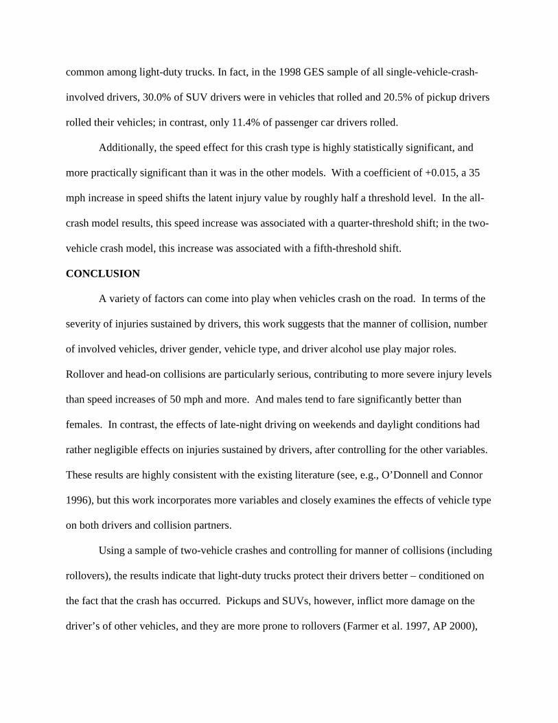
Additionally, the speed effect for this crash type is highly statistically significant, and

more practically significant than it was in the other models. With a coefficient of +0.015, a 35

mph increase in speed shifts the latent injury value by roughly half a threshold level. In the all-

crash model results, this speed increase was associated with a quarter-threshold shift; in the two-

vehicle crash model, this increase was associated with a fifth-threshold shift.

CONCLUSION

A variety of factors can come into play when vehicles crash on the road. In terms of the

severity of injuries sustained by drivers, this work suggests that the manner of collision, number

of involved vehicles, driver gender, vehicle type, and driver alcohol use play major roles.

Rollover and head-on collisions are particularly serious, contributing to more severe injury levels

than speed increases of 50 mph and more. And males tend to fare significantly better than

females. In contrast, the effects of late-night driving on weekends and daylight conditions had

rather negligible effects on injuries sustained by drivers, after controlling for the other variables.

These results are highly consistent with the existing literature (see, e.g., O’Donnell and Connor

1996), but this work incorporates more variables and closely examines the effects of vehicle type

on both drivers and collision partners.

Using a sample of two-vehicle crashes and controlling for manner of collisions (including

rollovers), the results indicate that light-duty trucks protect their drivers better – conditioned on

the fact that the crash has occurred. Pickups and SUVs, however, inflict more damage on the

driver’s of other vehicles, and they are more prone to rollovers (Farmer et al. 1997, AP 2000),

G G

which, as mentioned, result in very severe injuries. In fact, passenger cars roll about one-half as

often as pickups and one-third as often as SUVs. A more comprehensive model, which

simultaneously examine exposure and crash involvement, could assess whether drivers of light-

duty trucks are more at risk overall, by virtue of being more crash involved – and more likely to

rollover. Research should continue in this important area.

ACKNOWLEDGEMENTS

The authors wish to acknowledge the University of Texas’ Department of Civil

Engineering and the Luce Foundation for their support of this work.

G G

REFERENCES

Abdel-aty, M. A., Chen, C., and Schott, J. R. (1998) An assessment of the effect of driver age on

traffic accident involvement using log-linear models. Accident Analysis and Prevention, 30(6),

851–861.

Aljanahi, A. A. M., Rhodes, A. H., and Metcalfe, A.V. (1999) Speed, speed limits and road

traffic accidents under free flow conditions. Accident Analysis and Prevention, 31(2), 161-168.

AP (2000) “Automakers take aim at rollovers.” New York Times, Associated Press (May 23).

Ben-Akiva, M., and Lerman, S. R. (1985) Discrete Choice Analysis. Cambridge, Massachusetts;

MIT Press.

Chipman, M. L., MacGregor, A. G., Smiley, A. M., and Lee-Gosselin, M. (1992) Time vs.

distance as measures of exposure in driving surveys. Accident Analysis and Prevention, 24(6),

679-684.

Deyoung, David J., Peck, Raymond C., and Helander, Clifford J. (1997) Estimating the exposure

and fatal crash rates of suspended/revoked and unlicensed drivers in California. Accident

Analysis and Prevention, 29(1), 17-23.

Dobson, A., Brown, W., Ball, J., Powers, J., and McFadden, M. (1999) Women drivers’

behavior, socio-demographic characteristics and accidents. Accident Analysis and Prevention, 31

(5), 525-535.

G G

Doherty, S. T., Andrey, J. C. and MacGregor, C. (1998) The situational risks of young drivers:

The influence of passengers, time of day and day of week on accident rates. Accident Analysis

and Prevention, 30(1), 45-52.

Farmer, C. M., Braver, E. R., and Mitter, E. L. (1997) Two-vehicle side impact crashes: The

relationship of vehicle and crash characteristics to injury severity. Accident Analysis and

Prevention, 29(3), 399-406.

Gebers, M. A. (1998) Exploratory multivariable analyses of California driver record accident

rates. Transportation Research Record 1635, 72-80.

Greene, W. H. (2000) Econometric Analysis, Fourth Edition. New Jersey, Prentice Hall.

Hauer, E. and Hakkert, A. S. (1988). Extent and some implications of incomplete accident

reporting, Transportation Research Record 1185, 1-11.

Hu, P. S., Trumble, D. A., Foley, D. J., Eberhard, J. W., and Wallace, R. B. (1998) Crash risks of

older drivers: A panel data analysis. Accident Analysis and Prevention, 30(5), 569-581.

Ivan, J. N., Pasupathy, R. K. and Ossenbruggen, P. J. (1999) Differences in causality factors for

single and multi-vehicle crashes on two-lane roads. Accident Analysis and Prevention, 31(6),

695-704.

Karlaftis, M. G., and Tarko, A. P. (1998) Heterogeneity considerations in accident modeling.

Accident Analysis and Prevention, 31(1), 425-433.

Li, Lei, and Kim, Karl. (2000) Estimating driver crash risks based on the extended Bradley-Terry

model: an induced exposure method. J. Royal Statistical Society A 163 (2), 227-240.

G G

Lourens, P. F., Vissers, J. A. M. M., and Jessurun, M. (1999) Annual mileage, driving violations

and accident involvement in relation to drivers’ sex, age and level of education. Accident

Analysis and Prevention, 31 (1), 593-597.

McCarthy, Patrick, and Madanat, Samer. (1994) Highway Accident Data Analysis.

Transportation Research Record 1467, 44-49.

O’Donnell, C. J., and Connor, D. H. (1996) Predicting the severity of motor vehicle accident

injuries using models of ordered multiple choice. Accident Analysis and Prevention, 28 (6), 739-

753.

Ryan, G. A., Legge M., and Rosman, D. (1998) Age related changes in drivers’ crash risk and

crash type. Accident Analysis and Prevention, 30 (3), 379-387.

Shankar, V., Milton, J., and Mannering, F. (1997). Modeling accident frequencies as zero-altered

probability processes: An empirical inquiry. Accident Analysis and Prevention 29 (6), 829-837.

Zhang, J., Lindsay, J., Clarke, K., Robbins, G., and Mao, Y. (2000) “Factors affecting the

severity of motor vehicle traffic crashes involving elderly drivers in Ontario. Accident Analysis

and Prevention 32 (1), 117-125.

G G

Table 1. Description of Variables

Variable Type

Variable Title Description Mean SD

Dependent Variable

INJURYLEVEL 4 Crash categories: No injury (0), minor injury (1), severe injury (2), and fatal injury sustained by driver (3)

0.3108 0.5564

Driver Info. AGE Age of driver (years) 37.34 16.08

AGE2 Age squared 1433 1335

MALE Gender (1=Male, 0=Female) 0.6333 0.4819

ALCOHOL Police-reported alcohol involvement (1=Yes) 0.0430 0.2028

VIOLATOR Driver has a past traffic violation on record (1=Yes) 0.2954 0.4562

Vehicle Info. VEHAGE Vehicle age (1999 – model year) 7.9471 5.4595

PICKUP Driver driving a pick-up truck (1=Yes) 0.1323 0.3388

MINIVAN Driver driving a minivan (1=Yes) 0.0240 0.1531

SUV Driver driving a sport utility vehicle (1=Yes) 0.0558 0.2295

HDT Driver driving a heavy or medium-duty truck (1=Yes) 0.1029 0.3039

OTHER Driver driving some other type of vehicle (but not a passenger car) – e.g., motorcycles, full-sized vans, and buses (1=Yes)

0.0778 0.2679

OTHERPICKUP Collision partner (in two-vehicle crashes) is a pickup (1=Yes)

0.1341 0.3408

OTHERMINIVAN Collision partner is a minivan (1=Yes) 0.0209 0.1431

OTHERSUV Collision partner is an SUV (1=Yes) 0.0454 0.2081

OTHERHDT Collision partner is an HDT (1=Yes) 0.1049 0.3064

OTHEROTHER Collision partner is any other type of vehicle (but not a passenger car) (1=Yes)

0.0918 0.2888

Crash Info. HEADON (FRONT)

Head-on crash type (front-end impact for single-vehicle crashes) (1=Yes)

0.0190 (0.4556)

0.1365 (0.4980)

REAREND (BACK)

Rear-end crash type (back-end impact for single-vehicle crashes) (1=Yes)

0.3294 (0.1893)

0.4700 (0.3917)

ROLLOVER Rollover (1=Yes) 0.0343 0.1820

LEFTSIDE Left-side impact (1=Yes) 0.1666 0.3727

RIGHTSIDE Right-side impact (1=Yes) 0.1601 0.3667

SPEED Actual travel speed (mph) (as estimated in police record)

23.46 18.98

SPEEDOTHER Collision partner’s actual travel speed (mph) 23.46 18.98

Other Info. OCCUPANTS Number of occupants in driver’s vehicle (1=Yes) 1.424 0.8608

DAYLIGHT Daylight – including dusk and dawn (1=Yes) 0.7301 0.4439

FRIDAYLATE Friday late night (between Friday midnight & 4 am of next day) (1=Yes)

0.0085 0.0918

SATLATE Saturday late night (midnight to 4 am) (1=Yes) 0.0076 0.0870

SUNLATE Sunday late night (midnight to 4 am) (1=Yes) 0.0032 0.0562

G G

Table 2. Model Results for All Crashes

Variables W/o Speed Variable With Speed Variable Coefficient p-value Coefficient p-value Constant -0.4364 0.0000 -0.7240 0.0000 Driver AGE 4.046E-04 0.7412 6.485E-03 0.0006 AGE2 8.100E-06 0.5473 -3.947E-05 0.0572 MALE -0.2323 0.0000 -0.2640 0.0000 VIOLATOR -0.1024 0.0000 -0.0722 0.0000 ALCOHOL 0.3210 0.0000 0.2978 0.0000 Vehicle VEHAGE 7.101E-03 0.0000 7.226E-03 0.0000 SUV -0.1584 0.0000 -0.2220 0.0000 MINIVAN -0.1203 0.0000 -0.1318 0.0030 PICKUP -0.1719 0.0000 -0.1751 0.0000 HDT -0.5773 0.0000 -0.6005 0.0000 OTHER 0.1832 0.0000 0.1640 0.0000 Crash HEADON 0.5415 0.0000 0.6483 0.0000 REAREND -0.1598 0.0000 -0.0201 0.2666 ROLLOVER 0.9633 0.0000 0.8566 0.0000 LEFTSIDE -0.0153 0.2206 1.132E-03 0.9564 RIGHTSIDE -0.1866 0.0000 -0.1782 0.0000 SPEED 6.726E-03 0.0000 Others OCCUPANTS -8.397E-03 0.0862 -0.0101 0.1569 DAYLIGHT -0.0135 0.1767 -0.0199 0.2071 FRILATE 0.1088 0.0121 0.1729 0.0203 SATLATE 0.0596 0.2159 -0.0141 0.8610 SUNLATE 0.2369 0.0003 0.1379 0.2392 Thresholds

µ1 0.0000 - 0.0000 - µ2 1.1823 0.0000 1.1245 0.0000 µ3 2.2003 0.0000 2.2950 0.0000

Num. of observations 97,074 40,251 LRI 0.0451 0.0496

G G

Table 3. Model Results for Two-Vehicle Crashes

Variables W/o Speed Variable With Speed Variable Coefficient p-value Coefficient p-value Constant -0.5397 0.0000 -0.8624 0.0000 Driver AGE 3.171E-03 0.0352 7.030E-03 0.0071 AGE2 -1.411E-05 0.3877 -4.237E-05 0.1314 MALE -0.2665 0.0000 -0.2786 0.0000 VIOLATOR -0.0877 0.0000 -0.0394 0.0650 ALCOHOL 0.2435 0.0000 0.2399 0.0000 Vehicle VEHAGE 7.045E-03 0.0000 7.367E-03 0.0000 SUV -0.1915 0.0000 -0.2764 0.0000 MINIVAN -0.1549 0.0000 -0.2971 0.0000 PICKUP -0.2171 0.0000 -0.2667 0.0000 HDT -0.7743 0.0000 -0.8247 0.0000 OTHER 0.1103 0.0000 0.0916 0.0047 OTHERSUV 0.1458 0.0000 0.0340 0.4676 OTHERMINIVAN 0.0598 0.0893 -0.0685 0.3291 OTHERPICKUP 0.0935 0.0000 -1.584E-03 0.9563 OTHERHDT 0.5444 0.0000 0.3438 0.0000 OTHEROTHER 0.1439 0.0000 0.1681 0.0000 Crash HEADON 0.5870 0.0000 0.6819 0.0000 REAREND -0.1935 0.0000 -0.1480 0.0000 ROLLOVER 1.0908 0.0000 0.9046 0.0000 LEFTSIDE -0.0451 0.0032 -0.0635 0.0259 RIGHTSIDE -0.1933 0.0000 -0.2475 0.0000 SPEED 5.875E-03 0.0000 SPEEDOTHER 6.176E-03 0.0000 Others OCCUPANTS 2.268E-03 0.7061 -6.545E-03 0.5190 DAYLIGHT -0.0582 0.0000 -0.0338 0.1525 FRILATE 0.0414 0.5455 0.1250 0.4133 SATLATE 0.0776 0.2898 0.0539 0.7241 SUNLATE 0.3465 0.0010 0.0235 0.9268 Thresholds

µ1 0.0000 - 0.0000 - µ2 1.2290 0.0000 1.0834 0.0000 µ3 2.3272 0.0000 2.3522 0.0000

Num. of observations 65,510 20,382 LRI 0.0588 0.0682

G G

Table 4. Model Results for Single-Vehicle Crashes

Variables W/o Speed Variable With Speed Variable

Coefficient p-value Coefficient p-value

Constant -0.2009 0.0061 -0.9059 0.0000

Driver

AGE -0.0181 0.0000 -0.0163 0.0012

AGE2 1.510E-04 0.0000 1.824E-04 0.0016

MALE -0.1009 0.0000 -0.1530 0.0001

VIOLATOR -0.1331 0.0000 -8.283E-03 0.8282

ALCOHOL 0.4174 0.0000 0.3504 0.0000

Vehicle

VEHAGE 8.665E-03 0.0000 9.349E-03 0.0008

SUV 0.0322 0.4427 0.0126 0.8622

MINIVAN -0.1525 0.0390 -0.0690 0.5940

PICKUP 0.0217 0.4624 0.1321 0.0060

HDT 0.0398 0.3447 0.0588 0.3952

OTHER 0.5891 0.0000 0.7279 0.0000

Crash

ROLLOVER 0.7837 0.0000 0.6622 0.0000

FRONT 0.0337 0.3171 0.0794 0.1246

BACK -0.5647 0.0000 -0.2825 0.0190

LEFTSIDE -0.0356 0.4035 0.0112 0.8681

RIGHTSIDE -0.2406 0.0000 -0.1441 0.0233

SPEED 0.0152 0.0000

Others

OCCUPANTS -0.0433 0.0003 -0.0852 0.0000

DAYLIGHT 0.0243 0.2588 0.0548 0.1244

FRILATE 0.1354 0.0310 0.2426 0.0246

SATLATE 0.0541 0.4355 -0.0980 0.3780

SUNLATE 0.0993 0.2903 0.0923 0.5621

Thresholds

µ1 0.0000 - 0.0000 -

µ2 1.0908 0.0000 1.0309 0.0000

µ3 2.0908 0.0000 2.1859 0.0000

Num. of observations 16,420 5,715

LRI 0.0659 0.0868

age effect vs. age

G G

1 It should be noted that multinomial models were also run, allowing for additional flexibility in terms of a parameter space (so, for example, higher ages could contribute to a higher likelihood of fatal injuries and no injuries but lower likelihoods of severe and non-severe injury). Their results are quite consistent with the ordered-probit model results presented here (in terms of coefficient signs and magnitudes). A multinomial specification, however, does not recognize the clearly ordinal nature of the injury levels. So only the ordered probit results are provided below.