DROMO formulation for planar motions: solution to the Tsien problem

Hodei Urrutxua1 • David Morante1 • Manuel Sanjurjo-Rivo2 • Jesus Pelaez1

Abstract The two-body problem subject to a constant radial thrust is analyzed as a planar motion. The description of the problem is performed in terms of three perturbation methods: DROMO and two others due to Deprit. All of them rely on Hansen's ideal frame concept. An explicit, analytic, closed-form solution is obtained for this problem when the initial orbit is circular (Tsien problem), based on the DROMO special perturbation method, and expressed in terms of elliptic integral functions. The analytical solution to the Tsien problem is later used as a reference to test the numerical performance of various orbit propagation methods, including DROMO and Deprit methods, as well as Cowell and Kustaanheimo-Stiefel methods.

Keywords DROMO • Planar motion • Radial thrust • Tsien problem • Time regularization • Numerical propagation of orbits

1 Introduction

Planar motions in the perturbed two body problem (TBP) are frequently encountered in Celestial Mechanics. In many cases of interest, the perturbing forces considered are contained in the orbital plane, leading to orbits that remain confined in the same plane. These motions

EE3 Hodei Urrutxua hodei.urrutxua@upm.es

David Morante dmorante@ing.uc3m.es

Manuel Sanjurjo-Rivo msanjurj@ing.uc3m.es

Jesus Pelaez j.pelaez@upm.es

Space Dynamics Group (SDG-UPM), Technical University of Madrid, Pza. Cardenal Cisneros 3, 28040 Madrid, Spain

Space Dynamics Group (SDG-UPM), Bioengineering and Aerospace Engineering Department, Carlos III University, Avda. de la Universidad 30, 28911 Leganes, Madrid, Spain

are extremely interesting from an academical point of view due to their dynamical richness, but they are also important in the sense that many real life scenarios may be conveniently modeled as planar motions.

For instance, orbit repositioning, interplanetary transfer orbits or solar sailing are a few areas whose study often reduces to planar motions. Other examples regarding space situa­tional awareness applications have recently awakened a great interest, like deorbiting space debris or applying slow deflection trajectories for hazardous asteroid mitigation. All this kind of applications benefit from the study of planar motions.

Tsien (1953) studied continuous low-thrust trajectories for Earth escape from circular orbit by decomposing the thrust into radial and circumferential components, and analyzing each problem separately. In particular, he provided analytic solutions to the constant radial thrust problem, hereafter referred to as the Tsien problem. A comprehensive analysis of the problem is presented by Battin (1987) and Boltz (1991). It is found that there exists a limit value of the constant thrust that leads to a limit circular orbit. Below that value the trajectory is bounded, and above yields escape trajectories. Additionally, the problem may also be studied qualitatively from an energetic approach, which suffices to provide information on the escape conditions and the amplitude of the oscillations in the bounded case (Prussing and Coverstone-Carrol 1998). This study was later extended by Akella and Broucke (2002), who also found and classified periodic orbits and their stability using numerical methods. Years later Mengali and Quarta (2009) revisited the energetic approach for the case of an elliptic initial orbit. More recently, San-Juan et al. (2012) approached the problem by computing the general solution (for the bounded case only) from the Hamilton-Jacobi equation.

One of the reasons why the Tsien problem still catches the attention of researchers lies in the integrability of the problem, which admits closed-form solutions in terms of standard elliptic integrals: the radial time evolution depends on the incomplete elliptic integrals of the first and second kinds, and the orbit evolution is known to depend on the incomplete elliptic integral of the third kind (Akella 2000). However, all these solutions result in equations expressing the time as a function of the state variables, and not vice-versa, as would be desirable for mission design application purposes. Aware of this limitation, Quarta and Mengali (2012) managed to propose an explicit, albeit approximate, closed-form solution for the trajectory in the bounded case. It was not until very recently that Izzo and Biscani (2013) succeeded to find the first closed-form general explicit solution to the problem, relating the state variables to an anomaly, in terms of Weierstrass elliptic functions.

A yet unexplored path to tackle the Tsien problem is the use of alternative parameteri-zations of the equations of motion. Several propagation methods exist by means of which the governing equations may be reformulated in terms of unconventional variables or non-classical orbital elements. These formulations often include advantageous features such as time regularization, linearization, singularity-free state vectors, redundant sets of variables, or several of these features altogether. Although these methods are generally used for numer­ical orbit propagation purposes, many of them are not just suitable for analytic treatment, but rather enormously useful, offering a brand new and often more simple analytic approach to certain problems in Astrodynamics. One such formulation is the DROMO method (Pelaez et al. 2007), which is being actively developed and thoroughly tested for the past few years. The DROMO method happens to be related to a formulation proposed by Deprit (1975), and a variation of the latter studied by Palacios and Calvo (1996). The three of them are conceptually based on the ideal frame proposed by Hansen (1857) and have other properties in common, though their differences may have a huge impact in their numerical performance, and DROMO probably offers the best insight for analytical treatment. As a matter of fact, the DROMO formulation provides a theoretical framework where exact solutions may be

obtained, as for the Tsien problem, in a natural and often more straightforward way than with traditional approaches.

Hence, one contribution of this article consists of a novel solution to the Tsien problem, formulated in terms of DROMO variables, which leads to an exact and explicit analytical closed-form solution, where the state variables and the flight time are expressed as parametric functions, similarly to Izzo and Biscani (2013). The DROMO solution easily and naturally leads to the elliptic integrals that comprise the core of the solution, and do so in a much easier way than in other solutions available in the literature, since the required transformations and changes of variable are totally standard and no sophisticated constructions nor superior mathematical tools are needed. Also, this solution drawn from the DROMO formulation describes the three regimes of the Tsien problem in a unified manner, which is not always the case in other approaches. Besides, the solution preserves a clear physical meaning whilst providing new insight into the problem, as the solution is given in terms of an alternative parameterization of the state vector that pinpoints the evolution of the eccentricity vector and the so called ideal anomaly.

Another contribution corresponds to a performance assessment of different propaga­tion methods applied to the Tsien problem. When it comes to numerical orbit propagation, the performance—i.e. the relation between the computation speed and the accuracy of the numeric solution—becomes a great concern. The usual way of studying the performance of these methods is by setting up a benchmark problem and measuring the speed and accuracy of each method. Once the analytical solution is obtained for the Tsien problem, this may be used as a reference solution to build up test scenarios where to put the various propaga­tion methods to the test. Three different test cases are proposed, which have been designed to easily evaluate the performance while remaining representative of the different kinds of orbital motions that may exist in the Tsien problem. In particular, the DROMO formulation is tested along with the aforementioned Deprit and Palacios methods, as well as the Cowell and Kustaanheimo-Stiefel methods, in order to show a better picture that includes more widely used propagation methods and compare their performance to DROMO. The use of the Tsien problem for testing numerical propagators is new in the literature and may offer interest­ing conclusions, since scenarios may be proposed where the perturbation is not necessarily small.

The paper is organized as follows. Through Sects. 2-A the DROMO, Deprit and Palacios formulations are briefly introduced and their major differences are discussed. Then, the Tsien problem is stated in terms of DROMO variables (Sect. 5). The following Sect. 6, is devoted to derive an exact and explicit analytical closed-form solution to the Tsien problem. Finally, using the analytic solution to the Tsien problem as a baseline, a few test cases are proposed for the evaluation of several numerical propagation methods (Sect. 7), and some conclusions on their performances are drawn.

2 The DROMO formulation

The DROMO formulation provides an alternative parameterization of the orbital motion of a particle P, exposed to a perturbing acceleration ap, typically described in Cartesian coordinates by the non-dimensional equation

d 2 x x T~2 =—3+aP W d r z ri

Fig. 1 Geometric layout of the problem

k, zi h

A r JL-

where r is the non-dimensional time, r is the modulus of the non-dimensional position vector, x, and a certain characteristic length of the problem, lc, and angular velocity, a>c, are needed to turn the problem dimensionless.

The coordinates in Eq. (1) are referred to an inertial reference frame, J^ = {0\X\y\Z\}, centered at the primary body, 0\, and with an orientation given by the unit vectors ii , j i and ki (see Fig. 1).

The orbital frame, ff = {0\xyz}, is centered at the primary body, 0\, and with unit vectors defined as

x x x v i = —, k = , j = k x i

r |x x v|

where v is the non-dimensional velocity vector. Understanding the underlying geometrical meaning of DROMO requires the introduction

of an intermediate reference frame, Jf = {OiXnyHZH}, attached to the osculating orbital plane and initially coincident with the instantaneous perifocal frame, & = {0\xpypzp}. Some of the advantageous features of DROMO reside in the use of this intermediate frame. In fact, the motion can be viewed as a composition of two motions: (1) a rotation from the inertial frame to the intermediate frame with angular velocity U>HI, and (2) a rotation from the intermediate frame to the orbital frame with angular velocity <*>OH, such that

Wff/

&OH

r

A 1

h

where h is the non-dimensional orbital angular momentum. In absence of perturbations, com = 0 and the intermediate frame remains still in the inertial space. Hansen (1857) referred to this frame as ideal frame. In a perturbed environment though, the ideal frame or Hansen frame, Jf?, is no longer fixed, but instead evolves in a slower time scale.

The DROMO formulation replaces the non-dimensional Cartesian representation of the particle, (T; X, V), by the equivalent parameterization (a; r, fi, £2> ?3> i]u m, *73> m)- These DROMO variables have a clear geometrical meaning that is worth noting. f i and £2 a r e the projections of the instantaneous eccentricity vector, e, onto the Hansen ideal frame, M1, i.e.

t,\=e- cosQS), £2 = e • sinQS)

where fi is the angle between the eccentricity vector, e, and the unit vector in • The variable f3 = l/his the inverse ofthe orbital angular momentum. The variables 77; are the components of a quaternion that determines the attitude of the ideal frame, Jf?, with respect to the the inertial frame, J^. The DROMO method includes a Sundman transformation for regularizing the motion, such that the independent variable is not the time, r, but an ideal anomaly, a,

measured from the unit vector i# . Therefore, r must be calculated during the integration process, as a dependent integration variable.

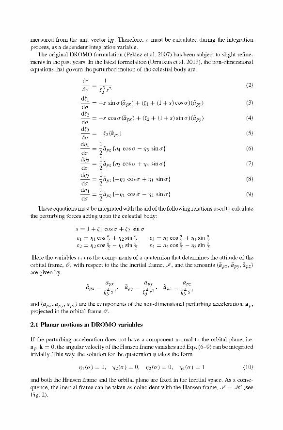
The original DROMO formulation (Pelaez et al. 2007) has been subject to slight refine­ments in the past years. In the latest formulation (Urrutxua et al. 2013), the non-dimensional equations that govern the perturbed motion of the celestial body are:

dr 1 (2)

dcr f| s2

—— =+s sma(apx) + (fi + (1 + s)cosa)(apy) (3) dcr

— = -s coscr (a px) + (£2 + (1 + s)sma)(apy) (4)

— = -&(apy) (5)

drji 1 ~T~ = ^apz (»?4 coscr - j?3 sincr} (6) dcr 2

d / ? 2 ! ~ r , - i rr, ~T~ = ^apz fe coscr + r]4 sincr} (7) dcr 2 d^3 1 -;— = ~aPZ {-f]2 coscr + r]i sincr} (8) dcr 2 dm _ 1 dcr ~ 2

5pZ {—T/i coscr — i]2 sincr} (9)

These equations must be integrated with the aid of the following relations used to calculate the perturbing forces acting upon the celestial body:

s = 1 + £i cos cr + £2 sin cr

gj = 77 j cos j + i]2 sin ^ £3 = 773 cos ^ + 7/4 sin ^ e2 = 772 cos §• — 771 sin ^ £4 = ^4 cos § — 773 sin |

Here the variables £; are the components of a quaternion that determines the attitude of the orbital frame, ff, with respect to the the inertial frame, ,y, and the amounts (apx, apy, apz) are given by

Upx-$s*' Py~^s^ pZ~^s^

and (apx, apy, apz) are the components of the non-dimensional perturbing acceleration, ap, projected in the orbital frame ff.

2.1 Planar motions in DROMO variables

If the perturbing acceleration does not have a component normal to the orbital plane, i.e. ap • k = 0, the angular velocity of the Hansen frame vanishes and Eqs. (6-9) can be integrated trivially. This way, the solution for the quaternion »/ takes the form

i?i(ff) = 0, 772(a) = 0, ri3(<r)=0, m(<r) = 1 (10)

and both the Hansen frame and the orbital plane are fixed in the inertial space. As a conse­quence, the inertial frame can be taken as coincident with the Hansen frame, ^ =. M1 (see Fig. 2).

Fig. 2 Scenario in a plane problem

The orbital frame is rotating around the fixed axis 0\z with an angular velocity crk and angular acceleration cfk; both values depend on the perturbing acceleration ap. So, the quaternion e that describes the attitude of the orbital frame relative to the inertial frame is given by

£\{<J) = e2(cr) a

0

e3(cr)

e4(cr)

sin 2 a

3 c 2 ?3*

Thus, the governing equations for the planar motion turn out to be

dr 1

da

dja dcr d?2 dcr d£s dcr

+s sin a(apx) + (fi + (1 + s) cos a)(apy)

-s cosa(apx) + (£2 + (1 + s) sina)(apy)

that have to be integrated along with the relations:

s = 1 + £i cos a + £2 sin cr

ei = £2 = 0 cr cr

S3 = sin —, £4 = cos — 2 2

and the order of the system is substantially reduced from eight to four.

(11)

(12)

(13)

(14)

(15)

(16)

(17)

3 The Deprit formulation

Deprit (1975) proposed a new set of elements to describe Keplerian motions subject to perturbing forces, which shares many similarities with the DROMO variables. This section briefly summarizes the fundamentals of the Deprit formulation, and highlights its differences with DROMO.

Let us consider the two-body problem given by Eq. (1). Deprit's formulation makes use of three different reference frames. The orbital frame, ff, is the same defined for DROMO in the previous section. However, whereas the inertial frame in the DROMO formulation, ,y, could

have any arbitrary orientation in space, the Deprit formulation expects an inertial frame, J^', that is initially aligned with the orbital frame. Also, one of the most remarkable similarities with DROMO is that Deprit's method also relies on a Hansen ideal frame. However, this ideal frames are not unique; any constant rotation in the orbital plane results in an equally valid ideal frame. So, the Hansen frame used by Deprit, 3^' = {Oyx^y^zu^u a n d its corresponding basis {in1, J H S k#<}, coincides by definition with both the orbital frame and the inertial frame, at the initial time.

Deprit solves Eq. (1) by proposing instead a parameterization of the problem with the eight non-classical elements (A.o, k\, k2, k^, G, C, S, F), termed by Deprit as ideal elements, since they are related to the concept of ideal reference frames.

The first four ideal elements, A.;, are the Euler-Rodrigues parameters of a finite rotation from the inertial frame ,y' to the ideal frame at epoch, M"', and the element G is in fact the non-dimensional angular momentum, h.

In order to set the osculating ellipse on the orbital plane, Deprit used the parameters C and S, which are the projection of the eccentricity vector in the ideal frame, M1', scaled by the angular momentum

e e C = —cosg, S=—sing

where g is the angle between the eccentricity vector and the unit vector ijji. Finally, Deprit introduced the variable F to determine the position of the particle in the

osculating ellipse. F stands for the mean anomaly reckoned from the axis Oix^1, and satisfies the relation F = M + g, where M represents the mean anomaly.

The equations that govern the perturbed motion of the particle in the Deprit formulation are:

-—=-apz — (kQcos9 - k^sin9) (18) d r 2 G dk2 1 r -—=-apz — (k0sm9+ k3cos9) (19) d r 2 G dk3 1 r

= —apz— (A.i sin.6 — k2 cos9) (20) d r 2 G dA.o 1 r —— =-apz — (-kicos6-k2sin6) (21) d r 2 G

(22)

(23)

(24)

AG

~dx dC

d r dS

d r dF

d r

T Clpy

= a / - j H <

= - a / • iH>

1 G2

a3'2 + 1 + Vl - e2

r- / ^ <L V ~ / d o

+ 2 — V I - e 2 ( — c G \ d r

/dS dC \ — cos 9 sin 0 I (25)

Vdr dr )

where (apx, apy, apz) correspond to the orbital frame components of the non-dimensional perturbing acceleration ap, e is the eccentricity and 9 represents the angle between the position vector x and the unit vector i#/. The value of a^, named as the effective perturbing force, is obtained as follows

»/ G2 i x (i x ap) (26)

Note that when the problem is planar, then apz = 0, the ideal frame becomes fixed in the inertial space and quaternion X becomes constant, so the set of equations reduces to Eqs. (22-25).

3.1 Comparison with DROMO formulation

DROMO and Deprit methods are built upon the ideal frame concept of Hansen (1857), but the ideal frames used in each formulation are different. Whereas for DROMO the ideal frame J$? is defined as coincident with the perifocal frame at the initial time, Deprit takes an ideal frame ,^f' initially aligned with the orbital frame instead. Therefore, these ideal frames differ by a constant finite rotation of value o$ (see Fig. 3), though both share the same fundamental properties.

In both methods, a set of Euler-Rodrigues parameters is used to describe the attitude of the corresponding ideal frame. Thus, quaternions X (Deprit) and »/ (DROMO) do not generally coincide, since the ideal frames they refer to are different, though they all vanish in the case of planar motions, as well as for the unperturbed case.

Deprit's ideal element G and the DROMO parameter £3 are equivalent, since they both relate to the orbital angular momentum, h. In fact, one is the inverse of the other, i.e. G = h = 1/fc.

Also, Deprit's elements (C, S) are equivalent to the DROMO elements (£1, £2), since they arise from the same concept: they represent the Cartesian projections of the eccentricity vector on the corresponding ideal frame. Note that, in Deprit, these values are also divided by the angular momentum G. So, these parameters fulfill the relation

1

G cos (To sin (To

— sin (To sin <ro

Finally, the major difference is encountered in the independent integration variable. The independent variable in DROMO is the ideal anomaly, a, as the result of a Sundman trans­formation. Therefore, as the time, r, does not appear explicitly, it has to be obtained along with the integration process as an additional dependent variable. Hence, the order of the sys­tem rises in one additional equation for DROMO. The three main consequences are: (1) the

Fig. 3 Geometrical relations between Deprit and DROMO

ky,(t) \x(t)

'M\

<V x,(t)

XH.(t)

XH(t)

formulation is unique for elliptic, parabolic and hyperbolic orbits, (2) no Kepler's equation or equivalent must be solved, and (3) an integration event or stop condition is required to finalize the integration when x = Xf is reached.

In Deprit's method, however, there is no such time regularization. So, the time, x, is the independent variable, and the additional parameter F is introduced to locate the particle P along the orbit. The use of F imposes two main drawbacks as compared to regularized methods like DROMO: (1) as F is a sort of mean anomaly, the resulting formulation is valid just for elliptic orbits, and (2) a modified Kepler's equation has to be solved in every integration step, which may handicap the performance.

4 Alternative Deprit formulation

It was Deprit himself who proposed an alternative formulation of the artificial satellite theory described in the previous section, in a discussion about linearization and the comparison between the methods of Laplace and Stiefel (Deprit et al. 1994). Palacios and Calvo (1996) revisited this alternative method and tested it in a series of scenarios.

Reference frames are defined and used in the same way as in the Deprit method. The set of non classical elements selected for this approach are seven, (Ao, Ai, A2, A3, G, /), T) , instead of eight. The first five are the same elements as in the previous Deprit method. The differences come up in the description of the motion within the orbital plane. Instead of following the evolution of the osculating ellipse, this alternative formulation pin-points the position of the artificial satellite in the orbital plane. This position is described in terms of the so-called projective coordinates. According to Palacios and Calvo (1996), a set of projective coordinates are p = 1/r, where r = |x| and 9 is an anomaly measured from the unit vector in', as described in the previous section. A regularization is performed and 9 replaces time as the independent variable. Thus, time x is a dependent integration variable in this formulation, as in DROMO. In addition, the characteristic magnitude of the acceleration is the same as in DROMO, thus, non-dimensional accelerations apx, apy and apz enter into the right hand side of the differential equations.

For the sake of completeness, the resulting set of equations of the alternative Deprit formulation, hereafter referred to as the Palacios formulation, are gathered below:

(27)

-A3 sin6») (28)

•A3 cos (9) (29)

A2cos<9) (30)

-A 2 s in60 (31)

(32)

dr

d0 ~ dAi

~d0 ~ dA2 _

dA3

~d0 ~ dA0

~d0 ~ dG

"d7 ~ d2p

1

1 -apz (k0cos9

1 -apz (A0srn6> •

1 -apz (Aisin6»

1 -apz (-Ai cos

GClpy

dp py

(33)

To sum up, the time evolution of the quaternions are computed in exactly the same way as in DROMO. Eqs. (2-9) and (27-33) are therefore analogous. The equations for time (27) and

angular momentum (32) are equivalent here and in DROMO. However, they are expressed in terms of their own set of elements. The motion within the orbital plane is governed by a second order differential equation in p. Reducing the order of the ODE system would yield a set of eight non-classical elements, as in the previous formulations. The solution for the unperturbed problem corresponds to a harmonic oscillator. Therefore, the analysis of the perturbed problem could benefit from the great amount of mathematical tools developed to tackle the well-known differential equation. For example, if apy = 0 and apx is assumed to be a periodic function in 9, the Hill equations are obtained, studied for the first time in the analysis of the lunar motion by Hill (1886).

5 The Tsien problem in DROMO formulation

A spacecraft in a circular orbit of radius RQ—circular velocity i^o^o with <DQ = /x/^o—i s

acted upon by a constant radial thrust ap = <2RUr starting at Jo­in order to introduce non-dimensional variables, the following characteristic magnitudes

are proposed:

lc = R0, coc = _j-^, r = coc(t-t0)

vc = coc Ro, ac --

Thus, the non-dimensional components of the perturbing acceleration in the orbital frame 0\xyz are

_ OR _ an _ „ _ „

ac R0cofi

The condition apz = 0 assures that the perturbed motion is planar.

5.1 Initial conditions

The standard procedure to obtain the initial values of the DROMO variables fails when e0 = 0. This is the case of the Tsien problem, and so the initial conditions should be calculated in a different way. The ip unit vector should point in the direction of the initial eccentricity vector; at first glance, and since eo = 0, one can choose any unit vector that lies on the orbital plane. However, a random choice of ip yields a discontinuous solution of the DROMO variables during the integration process. In order to avoid these discontinuities a careful selection of the ip vector should be carried out. By expanding the eccentricity vector around fo one gets

de e(r) = e0 + —

dr (t -10) +

to

where

de 1 , . — = — (a„ x h + v x (x x a„) dt JJ, '

To avoid discontinuities in the solution, the unit vector ip should be selected in the direction pointed by the derivative of e which is given by

de

d r = {2apyi-apxi}\t=0

:=0

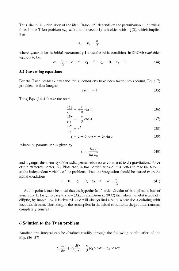
Thus, the initial orientation of the ideal frame, M1, depends on the perturbation at the initial time. In the Tsien problem apy = 0 and the vector ip coincides with — j(0), which implies that

<70 = V0 = —

where vo stands for the initial true anomaly. Hence, the initial conditions in DROMO variables turn out to be:

a = | : r = 0, ft = 0, ?2 = 0, £, = 1 (34)

5.2 Governing equations

For the Tsien problem, after the initial conditions have been taken into account, Eq. (17) provides the first integral

?3(<r) = 1 (35)

Thus, Eqs. (14-16) take the form

(36)

(37)

(38)

-?2sino- (39)

where the parameter e is given by

and it gauges the intensity of the radial perturbation <2R as compared to the gravitational force of the attractive center, 0\. Note that, in this particular case, it is better to take the time x as the independent variable of the problem. Thus, the integration should be started from the initial conditions:

r = 0 : ?i = 0, ?2 = 0, o = \ (41)

At this point it must be noted that the hypothesis of initial circular orbit implies no loss of generality. In fact, it is easy to show (Akella and Broucke 2002) that when the orbit is initially elliptic, by integrating it backwards one will always find a point where the osculating orbit becomes circular. Thus, despite the assumption in the initial conditions, the problem remains completely general.

6 Solution to the Tsien problem

Another first integral can be obtained readily through the following combination of the Eqs. (36-37)

d?i d?2 e C,\ — + C,2— = - (£i sin a - ?2 cos a)

dr dr 8

dfi dr d?2

dx da

dx s

=

^

=

£

+ -8 £

8 „2 s

1 +

sincr

coscr

ficos

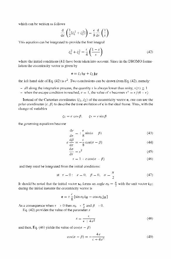
which can be written as follows

d

dr G[tf+fe2])=!£G) This equation can be integrated to provide the first integral

-2 , ,.2 £

( ^ ) ?i + G• = 4 I — ) (42)

where the initial conditions (41) have been taken into account. Since in the DROMO formu­lation the eccentricity vector is given by

e = £iiff + ?2J#

the left hand side of Eq. (42) is e2. Two conclusions can be drawn from Eq. (42), namely:

- all along the integration process, the quantity s is always lower than unity, s(r) < 1 - when the escape condition is reached, e = 1, the value of s becomes s* = e/(4 + e)

Instead of the Cartesian coordinates (£i, £2) of the eccentricity vector e, one can use the polar coordinates (e, p) to describe the time evolution of e in the ideal frame. Thus, with the change of variables

f 1 = e cos p, £2 = e sin /S

;he governing equations become

de e -r = + - s i n ( < r - / 3 ) dr 8 d£ e

e — = - jcosf f f - / 3 ) dr 8 da 2

dr ~S

s = 1 + ecos(cr — 3̂)

and they must be integrated from the initial conditions:

a t r = 0 : e = 0, 3̂ = 0, a = 2

(43)

(44)

(45)

(46)

(47)

It should be noted that the initial vector xo forms an angle CT0 = § with the unit vector in', during the initial instants the eccentricity vector is

e e = r - [sma0iH - cosa0jH]

o

As a consequence when r —»• 0 then o$ —»• ^ and f3 ̂ - 0. Eq. (42) provides the value of the parameter ,s

(48) e + 4 e 2

and then, Eq. (46) yields the value of cos(cr — p)

c o s ( a - £ ) = p-^r (49)

Since the right hand side of Eq. (49) is always negative the difference a — fi e [ j , ^ ] . As a consequence

s i n ( a - « = ± ^ f | , (50)

where A(e,e)= 16e4 + 8 ( e - 2 ) e 2 + e2 (51)

and the sign (+) should be taken when a — fi < jr. Finally, Eq. (43), the quotient of Eqs. (43^(4) and Eq. (45) lead to the following quadra­

tures:

8 r (e + 4 ^ r = T0 ± - / — (52)

P = fk>± - f = = (53)

o- = o - 0 ± 8 e / , , , (54) 7o (e+4£2 )^Hf^)

The solution of these equations depends on the particular value of the parameter e. There is an asymptotic solution when e = 1 that separates two different kinds of behaviors.

6.1 Bounded case e < 1

The biquadratic polynomial A(e, e) has four real roots. By introducing the value x2 = 1 — e > 0 these four roots are:

±\d + x), ±\d-x)

Let us introduce the change of variable

e = - (1 - x) sin6» where 9 e [0, jr] (55)

Note that when 9 goes from 0 to j,e increases and the value of sin(cr — fi) must be positive [see Eq. (43)]. When 9 goes from j to jr, however, e decreases and the value of sin(cr — fi) must be negative.

After the change of variable (55), Eq. (53) takes the form:

fe (1 + m) du P = Po+ . ==fi0 + (l + m)F(9,m)

Jo V 1 — sin a sin u

that is, fi is given by an elliptical integral of the first kind (see definition in "the Appendix"). Here the angle a e [0, j] and the modulus m e [0, 1] are given by

1 — X \ — m m = sin a = <£> x = (56)

1 + X l+m

Fig. 4 Left A typical trajectory in the case e < 1. Here e = 0.96. Note the choice of the 0\x\ axis relative to the initial position (point a). Right A periodic orbit. Here e R* 0.90812 and p = 4. q=3

A similar analysis can be carried out for the other equations. In summary, the following solution is obtained:

P = p0 + (l + m)F(9,m)

2 (1+m) TO +

m [(l + m)F(9,m)-E(9,m)]

a = (To + 2 (1 + m) 11(9, —m, m) m

sin0 (1+m)

(57)

(58)

(59)

(60)

where the functions F(9, m) and 11(9, —m, m) are elliptic integrals of the second and third kind, respectively. Essentially, the system (57-60) is a parametric representation of the tra­jectory taking as parameter the dummy variable 9. One must strictly stick to the definitions in "the Appendix", because the motion is periodic in 9 with this angle ranging in the interval 9 e [0,it].

The trajectory is contained in an annulus bounded by two circumferences of radii:

1 (inner). 1 + m (outer)

Figure 4 shows a typical trajectory for the value e = 0.96 (m = 2/3). The starting point is identified as a in the figure; the radial distance increases from r = 1 to r = rmax, where the trajectory is tangent to the outer circle (point b); then the radial distance decreases until r = 1 (point c) is reached again.

The integration starts at 9 = 0 from the initial conditions /3Q = 0, o$ = j and eo = 0.

During the arc ab the variable 9 describes the interval [0, j ] from 0 to j where the eccentricity

e reaches its maximum value, emax = m/(\ + m). In the second arc, be, the parameter 9 goes from j to jr.

In order to obtain the values of the variables at the end of one cycle, i.e. at 9 = it, the following classical relations of the elliptical integrals must be taken into account, for i j e N :

F (q —, m I = q FC(m)

E I q —, m I = q EC(m)

[7 lq — ,n,m\ = q IJC(n, m)

F(it,m) = 2FC(m)

E(jr, m) = 2EC(m)

n(it, n, m) = 2TTC(n, m)

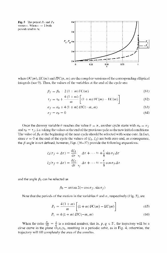
Fig. 5 The period Pr and Pa

versus e. When e —>• 1 both periods tend to oc

:

/ 1

/ 1 i "/ 1

js 1 : —-^

P O

where FC(m), EC (m) and77C(«, m) arc the complete versions of the corresponding elliptical integrals (see 9). Thus, the values of the variables at the end of the cycle are:

Pf = Po + 2(l + m)FC(m)

4(1 +m) Xf = x0 + (1 + m) FC(m) - EC(m)

af ffo + 4 (1 + m) nC(-m, m)

(61)

(62)

(63)

(64)

Once the dummy variable 9 reaches the value 9 = n, another cycle starts with o$ = a j and To = Xf, i.e. taking the values at the end of the previous cycle as the new initial conditions. The value of f$$ at the beginning of the next cycle should be selected with some care. In fact, since e = 0 at the end of the cycle the values of (£i, £2) a r e b°th zero and, as consequence, the fi angle is not defined; however, Eqs. (36-37) provide the following expansions:

d?i I e {,\(xf + Ax) = Ax + • • • ~ + - sinafAx

dr It/ 8 d?2| e

&(Xf + Ax) = Ax + • • • ~ — c o s a f AT dr IT/ 8

and the angle /3Q can be selected as

/So = arctan 2(— cos af, sin ay)

Note that the periods of the motion in the variables 9 and a, respectively (Fig. 5), are

4 ( l + m) ( l + m ) F C ( m ) - E C ( m )

4 ( l + m)77C(-m,m)

(65)

(66)

When the ratio j j = J is a rational number, that is, p, q e N, the trajectory will be a close curve in the plane 0\X\y\, resulting in a periodic orbit, as in Fig. 4; otherwise, the trajectory will fill completely the area of the annulus.

6.2 Unbounded case e > 1

When the parameter e is greater than unity, the spacecraft escapes from the gravitational field of the attractive center and the trajectory goes towards the infinity. There is also an analytical solution in terms of elliptical integrals, that can be obtained as follows.

Let us consider the Eq. (53) where now the sign (+) should be taken along the motion. To reduce the integral to the normal form of the elliptical integrals, the parameter x\r is introduced, such that

l + sinh2(2i/0

that is 1 xjr = -\n(^^\ + ^) (67)

and then the following change of variables can be performed

1 1 + cos a sin 9 -y/cosa — cos 9

2 1 — cos a sin 9 ^/cosa + cos 9

where the angle a e [0, j] is given by

(68)

This way,

where the

Eq. (53)

angle 9\

cos a = tanh'

becomes

P =

is given by

1 <A

Po +

9\ = arctan I

n = sin a = J1 — tanh4 x\i

(1 — cos a) du

yr

(-T=)> 6^K] \ y'cos a ) L IJ

(69)

A similar analysis for the remaining equations leads to the following solution

P = (l-cosof)[F(6>,m) -F(6»i,m)] (70)

' - ( l+cos 2a)(F(e»,m)-F(e»i ,m)) (1 + cosa) 2 \ 2

- ( E ( 0 , m ) -E(6»i,m))

cos^Vcosa — sin 9 /— —~ ~—

a O / 1

02 U i,m)]

V 1 — sin2 a sin2 9 (1 —cosa)) (71) s i n ( ? v c o s a + cos£ 2 /

- + (1-cosa) [¥{9,m)-¥{9i,m)]

- arctanI - — — - ^ — J — „ ~ ^ _ : j ! _ . ^ ^ ( 1 (1 — cos a) (cos2 9 — cosa sin2 9) \ /— I

2 y ' c o s a v l — sin2 a sin2 9 )

where the dummy variable 9 increases from the value 9 = 9\ given by (69) to the final value 9=9f=7t— 9\ (iaxi9f = — tan#i) in which the eccentricity, e, becomes infinite [see Eq. (68)]. The trajectory in this unbounded case has an infinite branch (an asymptote). A sketch is shown in Fig. 6 for the particular case e = 1.001. The right ascension of the asymptote is given by

n (Too = 1- 2(1 — cosa)[K(m) — F{9\, m)]

Fig. 6 Left A typical trajectory in the case e > 1. Here e = 1.001. Right A typical trajectory in the case e = 1. The final asymptotic radio is double of the initial radio. The final position is here for r = 100

6.3 Asymptotic case e = 1

The two behaviors described previously are separated by an asymptotic case that appears when the parameter e is strictly the unity (Fig. 6). It is easy to show that the analytical solution, in this case, is given by

P = ln l + 2e

l - 2 e l + 2e

4 In 8e l - 2 e

n 1 + 2e h In h 2 arctan(2e)

2 1 — 2e

(73)

(74)

(75)

The angle a — p is, obtained from the relations

4e COS((T — P)

l + 4e 2

and the coordinates (fi, £2) t u r n out to be:

4e 2

, sin(cr — P)

l - 4 e 2

l - 4 e 2

l + 4 e 2

6 =

-—r COS (7 + e l + 4 e 2

4e 2

7r sin cr — e

l + 4 e 2

l - 4 e 2

l + 4 e 2

The non-dimensional radial distance, r, is then

1

tfs l+Aez

since in the Tsien problem £3 = 1. From this relation, the value of the radial velocity can be obtained too, as well as the transversal component of the velocity, ra, as follows:

dr 1 - 4e2

vr dr 1 + 4e2

1 1

r2 ~ l + 4e 2

7 Numerical performance

Beyond the eventual analytical potential of DROMO, Deprit or Palacios formulations pre­sented in this paper, the most common application of these methods is the numerical propagation of orbits. These numerical propagators perform differently, in terms of speed and accuracy, depending on the considered problem or scenario, which is why numerical propagation methods are recurrently tested in the literature under as many different situa­tion as possible, in order to extract valuable and representative information on their overall performance (Stiefel and Scheifele 1971; Hull et al. 1972). The Tsien problem studied in this paper stands as an interesting benchmark, since knowing the analytical solution to the problem provides a simple and direct way to precisely measure the propagation errors of each method.

In this section, specific test cases are proposed for each of the three kinds of motions that may arise in the Tsien problem, depending on the value of the parameter e. For each test case, the numerical performance of the DROMO, Deprit and Palacios methods is studied. Additionally, both for completeness and to provide further insight, these performances are compared to the Cowell and Kustaanheimo-Stiefel (KS) methods too. These test cases are novel and the numerical results shown extend the comparison between different propagators to situations where the perturbing force is not necessarily small, i.e. e ^> 0. Such perturbed situations may find similarities with orbits near Lagrange points or perturbing third bodies, where the perturbation becomes important.

The following results were obtained coding these methods in Fortran and using a RKF 8(7) integrator on a i7-4771 @ 3.50GHz processor. Due to the sensitivity of some test cases and to remove numerical noise from the results, quadruple precision was used for all calculations.

7.1 Bounded case e < 1

The existence of periodic orbits in the case of bounded motions allows for a very practical way of evaluating the propagation errors. The trajectories turn into periodic orbits when the ratio 2F = f is a rational number with p, q e N; this condition comes from imposing that after q cycles, p revolutions around the attractive center are completed, i.e. that after a time r = q • PT has elapsed, the ideal anomaly fulfills

Of — (To = 1 • Pa = p • 2 71

Thus, after completing aperiodic orbit that revolves p times around the primary, the spacecraft should end up exactly at the starting point and with the starting velocity.

However, due to numerical propagation errors, the final point at the end of a given periodic orbit will not exactly coincide with the departing point, and the difference will grow or amplify after several orbits. Therefore, the difference between the final and starting points is a precise measure of the propagation error. The relation between this error and the required runtime or number of function calls quantifies the performance of the method.

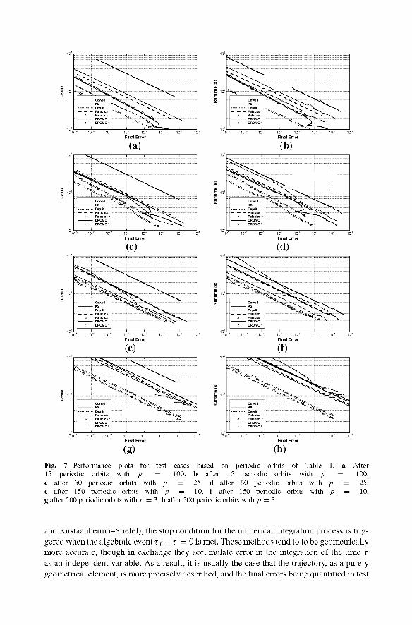
Each combination of integer values p, q leads to a periodic orbit with a different value of the parameter e, which proves to have substantial impact in the performance. In order to meaningfully cover the range of values of e, the periodic orbits of Table 1 are tested. For each of them n periodic orbits are propagated, such that n • p = 1500 revolutions around the center body are completed in total, and thus final errors are roughly comparable for all test cases. All calculations are started from the initial conditions xo = (0, 1), vo = (—1, 0) at to = 0, and propagated until tf = q • PT. The results are shown in Fig. 7, where the lines are parametric curves obtained by varying the integration tolerance.

Parameters

s = 0.96910737326711927753993356706719

Pa = 9.4247779607693797153879301498384

Pr = 17.341114976469186343237858003547

s = 0.57145103470048704045805933218600

Pa = 6.9813170079773183076947630739545

Pr = 8.4853562480397722140397555784208

s = 0.27880291829495551492454316703260

Pa = 6.5449846949787359134638403818324

Pr = 7.0844917149045398705499622671986

s = 0.077259034011890514247616700009811

Pa = 6.3466518254339257342679664308677

Pr = 6.4745400005887207701830926298562

Regarding the results, some conclusions can be drawn. All of these propagation methods perform better than Co well in terms of function calls, though for strongly perturbed scenarios some of the methods may end up being slower than Cowell. In fact, the performance of these methods is very dependent on the value of e.

Propagation methods based on perturbation techniques, such as DROMO or Deprit, show an outstanding performance in slightly perturbed environments (e <$; 1). As observed in Fig. 7a, b, DROMO, Deprit and Palacios perform better than Cowell and even the Kustaanheimo-Stiefel method. Particularly, Deprit ends up showing the smallest number of function calls for a given final error, though in terms of speed DROMO turns out to be faster. This is clearly a handicap of Deprit's method having to solve a modified Kepler's equation in every integration step, though this overhead could be lessened to some extent by solving Kepler's equation in more efficient ways than with a Newton-Raphson.

When moving to small, but somewhat larger values of e (Fig. 7c, d), three changes hap­pen: (1) Deprit's method loses the lead in the number of function calls, and the runtime deteriorates seriously becoming comparable to Cowell, (2) Kustaanheimo-Stiefel shows a comparative improvement in performance, making it the second best propagator, and (3) DROMO becomes both the fastest and most precise propagator in this range of values of e.

For moderate to high values of e (Fig. 7e-h), the perturbation becomes too strong, and the methods based on perturbations techniques, such as DROMO or Deprit, fall back in terms of performance; they still require less function calls than Cowell, though they become nearly as slow, and Deprit even breaks down in terms of speed. In this regime, the Palacios method seems to overtake DROMO and Deprit methods, performing faster and more precise. However, it is the Kustaanheimo-Stiefel method which performs best.

Remarkably, Kustaanheimo-Stiefel shows a more sustained behavior regardless of the magnitude of the perturbation e, i.e. while other methods show a better performances for nearly unperturbed scenarios, they deteriorate for growing values of e, whereas Kustaanheimo-Stiefel performs similarly for all 0 < e < 1, making it the best perform­ing propagator for moderate to high values of e.

Another interesting issue has to do with the stop condition. For these methods, the inte­gration is performed from To = 0 to tf = q • PT. Thus, for regularized methods whose independent integration variable is not the time but rather an anomaly (DROMO, Palacios

Table 1 Periodic orbits taken as test cases

Orbit

p = 3

q = 2

p=W

q = 9

p = 25

q = 24

p= 100

q = 99

, ^ - v >

"N^f^-v.

-v ^ ^ ^ o ^ ^ CowMl KS

OROMO o DROMO"

> 0 ' s ; ^~

.

» . l t ^ > & . . . *"* s T ^ ~ v .

""-• 3 '"'

(a) . . . . . . . . " S £ . ^ ^

rH;r„

•

• v ^ » ^

-

^ " ^ ^ 5 ;

' " • • * :

Fig. 7 Performance plots for test cases based on periodic orbits of Table 1. a After 15 periodic orbits with p = 100, b after 15 periodic orbits with p = 100, c after 60 periodic orbits with p = 25, d after 60 periodic orbits with p = 25, e after 150 periodic orbits with p = 10, f after 150 periodic orbits with p = 10, g after 500 periodic orbits with p = 3, h after 500 periodic orbits with p = 3

and Kustaanheimo-Stiefel), the stop condition for the numerical integration process is trig­gered when the algebraic event Xf — x = 0 is met. These methods tend to to be geometrically more accurate, though in exchange they accumulate error in the integration of the time x as an independent variable. As a result, it is usually the case that the trajectory, as a purely geometrical element, is more precisely described, and the final errors being quantified in test

cases are rather associated to timing or phasing errors. In other words, the final errors in position and velocity become larger than really are, because the integration is being stopped along the orbit sooner or later than it should, i.e. the propagator is introducing integration errors in the computation of time, that yield to errors in the final position and velocity. These errors could be compensated to some extent by using a finer integration tolerance for the variable x, than for the other variables.

However, since for this test case an analytical solution is available in terms of DROMO variables, then the stop condition may be imposed (in the usual way) to the independent integration variable, a, instead of time. Therefore, for the DROMO formulation the stop-condition tf = q • PT is equivalent to Of = o$ + q • Pa, where the latter does not require integration events and gets rid of the timing or phasing errors. This solution is shown in Fig. 7 labeled as DROMO*. For the particular geometry of this example, the independent variable of DROMO, a, and the independent variable of the Palacios method, 9, turn out to be identical, so the Palacios method may also be computed without timing errors (see Palacios* solution in Fig. 7). Both methods show a significant improvement in performance, of up to five orders of magnitude more precise for the same number of function calls in the highly perturbed case (Fig. 7g, h). This evidence suggests that the performance of these methods is highly sensitive to the proper integration of time and should be looked into more in detail in future work. Similarly, Kustaanheimo-Stiefel should experience a comparable boost in performance, though it is not included in these results because its independent integration variable is not equivalent to DROMO and Palacios methods1 so its new stop condition should be specifically computed.

Note that when computing the final errors of Fig. 7, the error norm includes both, the errors in position and velocity, but not in the physical time. If the timing or phasing error was to be considered too, then the performance of DROMO* would exactly match that of DROMO (idem for Palacios*). In fact, methods stopped with the stop condition Of do not account for the phasing error. On the other side, methods stopped with the stop condition Xf believe they have exactly reached the final time without phasing errors, i.e. x = Xf.ln truth, what happens is that when x reaches its final value, that physical time implicitly includes the accumulated integration error in the variable x. Hence, this phasing error is not revealed in the x variable (since the method assumes the current value of x is correct), but rather translates into position and velocity errors, i.e. the current state vector corresponds to the actual computed value of the physical time, but does not correspond to the true value of the physical time. Therefore, the difference between the DROMO and DROMO* performances (i.e., between using the stop condition in x or a) is a direct quantification of the phasing error.

7.2 Unbounded case e > 1

When the perturbation is large enough (e > 1) the escape condition is met and the motion turns unbounded. After spiraling out slowly approaching the asymptotic circular orbit of radius r = 2, the perturbation is strong enough to make the spacecraft escape away, approach­ing an asymptotic branch, as observed in Fig. 6. The larger the perturbation, the fastest the escape occurs. Therefore, from the point of view of putting the numerical propagators to the test, the most interesting regime, i.e. where the problem is most sensitive, is where the value of e is extremely close to the unity.

Whereas DROMO and Palacios are time-regularized using a second order Sundman transformation, Kustaanheimo-Stiefel uses a first order transformation instead.

Fig. 8 Exact and numerical solutions (Cowell) with varying integration tolerances for S = 1(T17

For convenience, let the non-dimensional perturbing force be rewritten as

£ = 1+8

When 8 = 0 the trajectory reaches the asymptotic circular orbit and—ideally—remains there forever. However, when the value of 8 is infinitesimal but non-zero, then the spacecraft revolves several times around the center body, closely following the asymptotic circular orbit, until eventually the escape occurs. When that happens, the trajectories head to infinity, approaching a radial asymptotic branch. As the value of 8 approximates the integration tolerance, the problem becomes increasingly sensitive and numerical errors make the escape trajectory to follow a different asymptotic radial branch, as illustrated in Fig. 8. Hence, it is most compelling to study how propagators struggle with values 8^1.

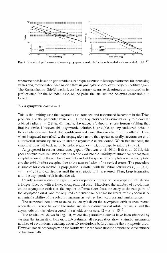
An easy way to quantify the error of the numerical solutions versus the exact, analytic solution, is to monitor the convergence of the right ascension—polar angle—of the asymptotic branch and compare it to the theoretical value. To guarantee that the spacecraft can be assumed to have reached the asymptotic branch, one would need to keep integrating until its polar angle, <p, remains unchanged—or below a reasonable threshold—in two subsequent integration steps. This, however, puts the focus on the angular error while paying no attention at the propagation of the radial distance. Therefore, an indirect way—the one we propose— of quantifying integration errors is to integrate until the spacecraft crosses a predefined circumference of arbitrary radius (we propose r = 1000). This way, the radial error is also indirectly accounted for. Additionally, as no timing errors are measured, the test problem becomes purely geometric, and thus the results become independent from the stop condition criteria discussed in the previous test case. In fact, all propagators should be stopped when the circumference crossing event (i.e. r — 1000 = 0) is triggered. For this case (r = 1000), a value of 8 = 10~17 and initial conditions xo = (0, 1), vo = (—1, 0), the reference final value is

<pf = -28.36185475050014°

Results are shown in Fig. 9 for the same propagators studied before. The first observation that should be noted is that Deprit's method fails at the very moment the trajectory becomes parabolic/hyperbolic, since the formulation is only valid for elliptic motions. This is a feature that many orbit propagation methods share and could result in the impossibility of integrating strongly perturbed problems where the nature of the orbit may evolve into non-elliptic.

Regarding the performance of the remaining methods, Palacios shows the best combination of speed and precision, while DROMO holds second best. As opposed to the previous test case,

Exact Tol = 18-19 Tol = 18-18 Tol = 1e-17 Tol = 1e-ie

10"10 10"8 1 0 ^ 1 0 ^ 10"2 10° 102 10"10 10"8 1 0 ^ 1 0 ^ 10"2 10° 10 s

Final Error (deg) Final Error (deg)

Fig. 9 Numerical performance of several propagation methods for the unbounded test case with 5 = 10

where methods based on perturbations techniques seemed to loose performance for increasing values of e, for the unbounded motion they surprisingly become extremely competitive again. The Kustaanheimo-Stiefel method, on the contrary, seems to deteriorate as compared to its performance for the bounded case, to the point that its runtime becomes comparable to Co well.

7.3 Asymptotic case e = 1

This is the limiting case that separates the bounded and unbounded behaviors in the Tsien problem. For the particular value e = 1, the trajectory tends asymptotically to a circular orbit of radius r = 2 (Fig. 6). Ideally, the spacecraft should remain forever orbiting that limiting circle. However, this asymptotic solution is unstable, so any undesired noise in the calculations may break the equilibrium and cause this circular orbit to collapse. Thus, when integrated numerically, the propagation errors that appear naturally, accumulate until a numerical instability shows up and the asymptote is abandoned. When this happens, the spacecraft may fall back in the bounded region (e < 1), or escape to infinity (e > 1).

As proposed in earlier conference papers (Urrutxua et al. 2011; Bail et al. 2011), this peculiar dynamical behavior may be used to evaluate the stability of numerical propagators, simply by counting the number of revolutions that the spacecraft completes on the asymptotic circular orbit, before escaping due to the accumulation of numerical errors. The procedure is simple: for each method, a propagation is started with the initial conditions xo = (0, 1), vo = (—1,0) and carried out until the asymptotic orbit is entered. Then, keep integrating until the asymptotic orbit is abandoned.

Clearly, a more accurate integration scheme permits to describe the asymptotic orbit during a longer time, or with a lower computational load. Therefore, the number of revolutions on the asymptotic orbit (i.e. the angular difference Aa from the entry to the exit point of the asymptotic orbit) and the required computational cost are measures of the goodness or numerical stability of the orbit propagators, as well as their accuracy and performance.

The numerical condition to detect the entry/exit on the asymptotic orbit is encountered when the difference between the instantaneous non-dimensional orbital radius, x, and the asymptotic orbit is below a certain threshold. In our case, |2 — x| < 10~3.

The results are shown in Fig. 10, where the parametric curves have been obtained by varying the integration tolerance. Interestingly, all propagators show a similar maximum number of revolutions, reaching about 10 revolutions before leaving the asymptotic orbit. However, not all of them provide the results within the same runtime or with the same number of function calls.

102 105 101 105 106 10' 10"1 10° 101 10s

Fcalls Runtime (s)

Fig. 10 Numerical performance of several propagation methods for the asymptotic case, e = 1

At the light of the results, the Palacios' method clearly outperforms all other propagators, since it reaches any number of revolutions on the asymptotic orbit considerably faster and with less function calls than any other method in the benchmark. The reason for this notorious advantage of Palacios, even compared with so similar methods as DROMO or Deprit, is not yet fully understood though. In any case, and despite the high value of the perturbation, DROMO remains the second best performing propagator, as in the unbounded test problem. Deprit's method, however, even if it takes as many function calls as Kustaanheimo-Stiefel, it takes even longer than Cowell to compute, handicapped by the overhead of solving Kepler's equation.

8 Conclusions

An explicit, analytic solution to the Tsien problem—constant radial thrust problem—is pro­vided. This general, closed form solution is expressed in terms of DROMO variables, allowing a parametric representation of the state vector as a function of elliptic integral functions. The solution is formally different for each of the three kinds of motions that may exist in the Tsien problem, i.e. bounded, unbounded or asymptotically circular motions.

These results show that these unconventional formulations, like DROMO, are not solely restricted to the domain of numeric orbit propagation, but they may be powerful tools for analytic applications too, allowing for new approaches to problems in celestial mechanics.

Also, the Tsien problem is numerically approached. Making use of the exact, analytic solution, three test problems—one per each kind of motion—are proposed in the framework of the Tsien problem, with the purpose of evaluating the performance of numerical orbit propagation methods. The DROMO, Deprit, Palacios, Kustaanheimo-Stiefel and Cowell methods were tested.

The results show a great dependence on the magnitude of the perturbation, and in particular a different behavior for the bounded and unbounded motions. For bounded and slightly perturbed motions, propagators based on perturbation techniques show the best performance, though Deprit's method is clearly handicapped by the overhead of solving Kepler's equation. The performance of DROMO is remarkable for slightly to moderately perturbed cases, but for highly perturbed motions the Kustaanheimo-Stifel method performs best, closely followed by the Palacios method. For unbounded motions—and in spite of the strong perturbations— Palacios and DROMO are the two best performing methods, in this same order. The Kusta­anheimo-Stiefel method seems to fall back, whereas Deprit's method is not even applicable, as the motion becomes hyperbolic. More particularly, in the limit case between bounded and unbounded motions—asymptotically circular motion—the Palacios method shows an outstanding performance, substantially better than any other tested propagator.

Acknowledgments This work is part of the research project entitled "Dynamical Analysis, Advanced Orbit Propagation and Simulation of Complex Space Systems" (ESP2013-41634-P) supported by the Spanish Min­istry of Economy and Competitiveness. Authors thank to the Spanish Government for its financial support. The work of Hodei Urrutxua is also supported by a grant of the Technical University of Madrid (UPM); Mr. Urrutxua thanks UPM for its support.

9 Appendix: Elliptic functions

The derivations on the article make extensive use of elliptic function. For completeness, the following definitions of the elliptic functions are provided:

fe du F(9,m)= / (76)

Jo V l - » i sin u

E(0,m)= / V l - m2 sin2 u du (77) Jo fe du

II(9,n,m)= (78) Jo (1 — n sin M)V 1 — m2 sin u

/it \ /* 2 du FC(m) = F ( - , m ) = / — (79)

V 2 ' io V 1 - / B 2 sin2 u

2 V l - m 2 sin2wdw (80)

nC(n,m) = n(-,n,m\ (81)

where the modulus m, in our problem, is given by Eq. (56).

References

Akella, M.R.: On low radial thrust spacecraft motion. J. Astronaut. Sci. 48(2-3), 149-161 (2000) Akella, M.R., Broucke, R.A.: Anatomy of the constant radial thrust problem. J. Guid. Control Dyn. 25(3),

563-570 (2002). doi:10.2514/2.4917 Battin, R.H.: An Introduction to the Mathematics and Methods of Astrodynamics. AIAA Education Series,

New York (1987) Bau, G., Huhn, A., Urrutxua, H., Bombardeili, C, Pelaez, J.: Dromo: a new regularize orbital propagator.

In: International Symposium on Orbit Propagation and Determination, IMCCE, Lille, France, 26-28 September (2011)

Boltz, F.W.: Orbital motion under continuous radial thrust. J. Guid. Control Dyn. 14(3), 667-670 (1991). doi:10.2514/3.20690

Deprit, A.: Ideal elements for perturbed Keplerian motions. J. Res. Natl. Bur. Stand. B Math. Sci. 79B(1 and 2), 1-15 (1975)

Deprit, A., Elipe, A., Ferrer, S.: Linearization: Laplace vs. Stiefel. Celest. Mech. Dyn. Astron. 58(2), 151-201 (1994). doi:10.1007/BF00695790

Hansen, PA.: Auseinandersetzung einer zweckmassigen Method zur Berechnung der absoluten Storungen der Kleinen Planeten. Abh der Math-Phys CI der Kon Sachs Ges der Wissensch 5, 41-218 (1857)

Hill, G.: On the part of the motion of the lunar perigee which is a function of the mean motions of the Sun and Moon. Acta Math. 8(1), 1-36 (1886). doi:10.1007/BF02417081

Hull, T, Enright, W., Fellen, B., Sedgwick, A.: Comparing numerical methods for ordinary differential equa­tions. SIAM J. Numer. Anal. 9, 603-637 (1972)

Izzo, D., Biscani, F : Solution of the constant radial acceleration problem using Weierstrass elliptic and related functions. arXiv:1306.6448 (2013)

Mengali, G., Quarta, A.A.: Escape from elliptic orbit using constant radial thrust. J. Guid. Control Dyn. 32(3), 1018-1022 (2009). doi:10.2514/1.43382

Palacios, M., Calvo, C : Ideal frames and regularization in numerical orbit computation. J. Astron. Sci. 44(1), 63-77(1996)

Pelaez, J., Hedo, J.M., de Andres, PR.: A special perturbation method in orbital dynamics. Celest. Mech. Dyn. Astron. 97, 131-150 (2007). doi:10.1007/sl0569-006-9056-3

Prussing, J., Coverstone-Carrol, V.: Constant radial thrust acceleration redux. J. Guid. Control Dyn. 21(3), 516-518 (1998). doi:10.2514/2.7609

Quarta, A.A., Mengali, G.: New look to the constant radial acceleration problem. J. Guid. Control Dyn. 35(3), 919-929 (2012). doi:10.2514/1.54837

San-Juan, J.F., Lopez, L.M., Lara, M.: On bounded satellite motion under constant radial propulsive acceler­ation. Math. Prob. Eng. 2012, 1-12 (2012). doi:10.1155/2012/680394. (iD 680394)

Stiefel, E.L., Scheifele, G.: Linear and regular celestial mechanics. Springer, Berlin (1971). doi:10.1007/ 978-3-642-65027-7

Tsien, H.S.: Take-off from satellite orbit. J. Am. Rocket Soc. 23, 233-236 (1953). doi:10.2514/8.4599 Urrutxua, H., Bombardeili, C, Pelaez, J.: High fidelity models for orbit propagation: Dromo vs. Stormer-

Cowell. In: European Space Surveillance Conference, INTA HQ, Madrid, Spain, 7-9 June (2011) Urrutxua, H., Sanjurjo-Rivo, M., Pelaez, J.: Dromo propagator revisited. In: Advances in the Astronautical

Sciences, 23rd AAS/AIAA Space Flight Mechanics Meeting Proceedings, Kauai, Hawai, USA, vol. 148, pp. 1809-1828, aAS 13-488 (2013)