reduction. NMF finds applications in text mining [30], image/video
processing [19], and analysis of social networks [34]. Unlike gen-
eral matrix factorization (MF), NMF restricts the two output matrix
factors to be nonnegative. Nonnegativity is inherent in the feature
space of many real-world applications, therefore the resulting fac-
tors can have a natural interpretation. Specifically, the goal of NMF
is to decompose a huge matrixM ∈ Rm×n+ into the product of two
Permission to make digital or hard copies of all or part of this work for personal or classroom use is granted without fee provided that copies are not made or distributed for profit or commercial advantage and that copies bear this notice and the full citation on the first page. Copyrights for components of this work owned by others than ACM must be honored. Abstracting with credit is permitted. To copy otherwise, or republish, to post on servers or to redistribute to lists, requires prior specific permission and/or a fee. Request permissions from [email protected].
niques, and introduces thematrix sketching technique. OurDSANLS
algorithm is presented in Section 3. Detailed theoretical analysis of
DSANLS algorithm is discussed in Section 4. Section 5 evaluates
DSANLS. Finally, Section 6 concludes the paper.
2 BACKGROUND AND RELATEDWORK2.1 NMF AlgorithmsWithin two-block coordinate descent schemes (exact or inexact,
shown as Algorithm 1), different subproblem solvers are proposed.
Algorithm 1: Two-Block Coordinate Descent: Framework of
Most NMF Algorithms
initialize U0 ≥ 0, V0 ≥ 0;
for t = 0 to T − 1 doUt+1 ← update(M , Ut , Vt );Vt+1 ← update(M , Ut+1, Vt );
endreturn UT and VT
The first widely used update rule is Multiplicative Updates (MU),
which was first applied for solving NLS problems in [6]. Later, MU
was rediscovered and used for NMF in [21]. MU is based on the
majorization-minimization framework. Its application guarantees
that the objective function monotonically decreases [6, 21].
Another extensively studied method is alternating nonnegative
least squares (ANLS), which represents a class of methods where
the subproblems forU andV are solved exactly following the frame-
work described in Algorithm 1. ANLS is guaranteed to converge
to a stationary point [10] and has been shown to perform very
well in practice with active set [16, 18], projected gradient [24],
quasi-Newton [41], or accelerated gradient [12] methods as the
subproblem solver.
Hierarchical alternating least squares (HALS) [4] solves each
NLS subproblem using an exact coordinate descent method that
updates one individual column ofU at a time. The optimal solutions
of the corresponding subproblems can be written in a closed form.
2.2 Distributed NMFParallel NMF algorithms are well studied in the literature [13, 36].
However, different from a parallel and single machine setting, data
sharing and communication have considerable cost in a distributed
setting. Therefore, we need specialized NMF algorithms for massive
scale data handling in a distributed environment. The first method
in this direction [25] is based on the MU algorithm. It mainly fo-
cuses on sparse matrices and applies a careful partitioning of the
data in order to maximize data locality and parallelism. Later, Cloud-
NMF [23], a MapReduce-based NMF algorithm similar to [25], was
implemented and tested on large-scale biological datasets. Another
distributed NMF algorithm [40] leverages block-wise updates for
local aggregation and parallelism. It also performs frequent updates
using whenever possible the most recently updated data, which is
more efficient than traditional concurrent counterparts. Apart from
MapReduce implementations, Spark is also attracting attention for
its advantage in iterative algorithms, e.g., using MLlib [28]. Finally,
there are implementations using X10 [11] and on GPU [27].
Themost recent and relatedwork in this direction isMPI-FAUN [14,
15], which is the first implementation of NMF using MPI for inter-
processor communication. MPI-FAUN is flexible and can be utilized
for a broad class of NMF algorithms that iteratively solve NLS sub-
problems including MU, HALS, and ANLS/BPP. MPI-FAUN exploits
the independence of local update computation for rows ofU andV
to apply communication-optimal matrix multiplication. In a nut-
shell, the full matrix M is split across a two-dimensional grid of
processors and multiple copies of bothU andV are kept at different
nodes, in order to reduce the communication between nodes during
the iterations of NMF algorithms.
2.3 Matrix SketchingMatrix sketching is a technique that has been previously used in
numerical linear algebra [9], statistics [32] and optimization [33].
Its basic idea is described as follows. Suppose we need to find a
solution x to the equation:
Ax = b, (A ∈ Rm×n , b ∈ Rm ). (3)
Instead of solving this equation directly, in each iteration of matrix
sketching, a random matrix S ∈ Rd×m (d ≪m) is generated, andwe instead solve the following problem:
(SA)x = Sb . (4)
Obviously, the solution of (3) is also a solution to (4), but not vice
versa. However, the problem size has now decreased fromm × n to
d×n.With a properly generated randommatrix S and an appropriatemethod to solve subproblem (4), it can be guaranteed that we will
progressively approach the solution to (3) by iteratively applying
this sketching technique.
To the best of our knowledge, there is only one piece of pre-
vious work [38] which incorporates dual random projection into
the NMF problem, in a centralized environment, sharing similar
ideas as SANLS, the centralized version of our DSANLS algorithm.
However, Wang et al. [38] did not provide an efficient subprob-
lem solver, and their method was less effective than non-sketched
methods in practical experiments. Besides, data sparsity was not
taken into consideration in their work. Furthermore, no theoreti-
cal guarantee was provided for NMF with dual random projection.
In short, SANLS is not same as [38] and DSANLS is much more
than a distributed version of [38]. The methods that we propose
in this paper are efficient in practice and have strong theoretical
guarantees.
3 DSANLS: DISTRIBUTED SKETCHED ANLS3.1 NotationsFor a matrix A, we use Ai :j to denote the entry at the i-th row and
j-th column of A. Besides, either i or j can be omitted to denote
a column or a row, i.e., Ai : is the i-th row of A, and A:j is its j-thcolumn. Furthermore, i or j can be replaced by a subset of indices.
For example, if I ⊂ {1, 2, . . . ,m}, AI : denotes the sub-matrix of Aformed by all rows in I , whereas A:J is the sub-matrix of A formed
by all columns in a subset J ⊂ {1, 2, . . . ,n}.
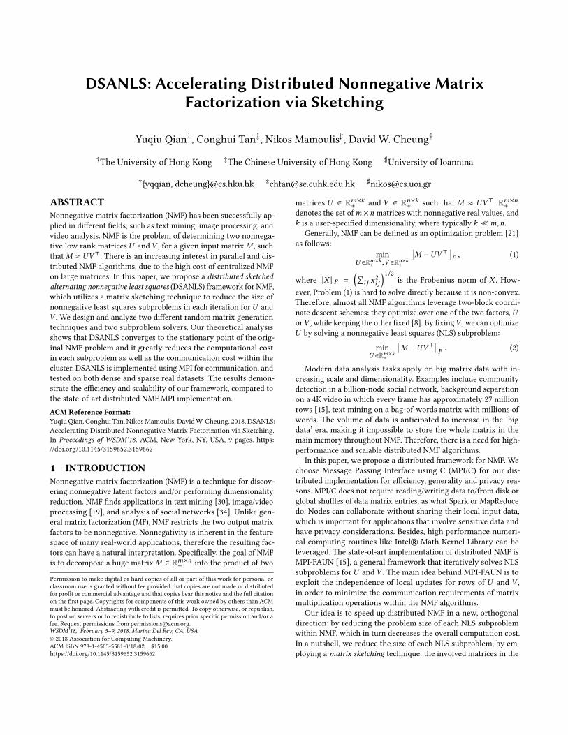
3.2 Data PartitioningAssume there are N computing nodes in the cluster. We partition
the row indices {1, 2, . . . ,m} of the input matrixM into N disjoint
sets I1, I2, . . . , IN , where Ir ⊂ {1, 2, . . . ,m} is the subset of rowsassigned to node r , as in [25]. Similarly, we partition the column
indices {1, 2, . . . ,n} into disjoint sets J1, J2, . . . , JN and assign col-
umn set Jr to node r . The number of rows and columns in each
node are near the same in order to achieve load balancing, i.e.,
|Ir | ≈m/N and |Jr | ≈ n/N for each node r . The factor matricesUandV are also assigned to nodes accordingly, i.e., node r stores andupdatesUIr : and VJr : as shown in Figure 1.
Figure 1: Data partitioning to N nodesData partitioning in distributed NMF differs from that in parallel
NMF. Previous works on parallel NMF [13, 36] choose to partitionUandV along the long dimension, but we adopt the row-partitioning
ofU and V as in [25]. To see why, take theU -subproblem (2) as an
example and observe that it is row-independent in nature, i.e., the
r -th row block of its solutionUIr : is given by
UIr : = arg min
UIr :∈R|Ir |×k+
MIr : −UIr :V⊤ 2
F (5)
and thus can be solved independently without referring to any
other row blocks of U . The same holds for the V -subproblem. In
addition, no communication is needed concerningM when solving
(5) becauseMIr : is already present in node r .On the other hand, solving (5) requires the entireV of size n × k ,
meaning that every node needs to gather V from all other nodes.
This process can easily be the bottleneck of a naive distributed
ANLS implementation. As we will explain shortly, our DSALNS
algorithm alleviates this problem, since we use a sketched matrix
of reduced size instead of the original complete matrix V .
3.3 SANLS: Sketched ANLSTo better understand DSANLS, we first introduce the Sketched
ANLS (SANLS), i.e., a centralized version of our algorithm. Recall
that in section 2.1, at each step of ANLS, eitherU orV is fixed andwe
solve a nonnegative least square problem (2) over the other variable.
Intuitively, it is unnecessary to solve this subproblem with high
accuracy, because we may not have reached the optimal solution
for the fixed variable so far. Hence, when the fixed variable changes
in the next step, this accurate solution from the previous step will
not be optimal anymore and will have to be re-computed. Our idea
is to apply matrix sketching for each subproblem, in order to obtain
an approximate solution for it at a much lower computational and
communication cost.
Specifically, suppose we are at the t-th iteration of ANLS, and
our current estimations forU andV areU tandV t
respectively. We
must solve subproblem (2) in order to update U tto a new matrix
U t+1. We apply matrix sketching to the residual term of subproblem
(2). The subproblem now becomes:
min
U ∈Rm×k+
MSt −U(V t⊤St
) 2
F , (6)
where St ∈ Rn×d is a randomly-generated matrix. Hence, the
problem size decreases from n × k to d × k . d is chosen to be much
smaller than n, in order to sufficiently reduce the computational
cost1. Similarly, we transform the V -subproblem into
min
V ∈Rn×k+
M⊤S ′t −V (U t⊤S ′t
) 2
F , (7)
where S ′t ∈ Rm×d′
is also a random matrix with d ′ ≪m.
3.4 DSANLS: Distributed SANLSNow, we come to our proposal: the distributed version of SANLS
called DSANLS. Since the U -subproblem (6) is the same as the
V -subproblem (7) in nature, here we restrict our attention to the
U -subproblem. The first observation about subproblem (6) is that
it is still row-independent, thus node r only needs to solve
min
UIr :∈R|Ir |×k+
(MSt)Ir :−UIr :
(V t⊤St
) 2
F.
For simplicity, we denote
Atr ,(MSt
)Ir :
and Bt , V t⊤St , (8)
and the above subproblem can be written as:
min
UIr :∈R|Ir |×k+
Atr −UIr :Bt 2
F . (9)
Thus, node r needs to know matrices Atr and Bt in order to solve
the subproblem.
For Atr , by applying matrix multiplication rules, we get
Atr =(MSt
)Ir := MIr :S
t
Therefore, if St is stored at node r , Atr can be computed without
any communication.
On the other hand, computing Bt =(V t⊤St
)requires communi-
cation across the whole cluster, since the rows ofV tare distributed
across different nodes. Fortunately, if we assume that St is storedat all nodes again, we can compute Bt in a much cheaper way.
Following block matrix multiplication rules, we can rewrite Bt as:
Bt = V t⊤St
=
[(V tJ1:
)⊤· · ·
(V tJN :
)⊤] StJ1:
...
StJN :
=
N∑r=1
(V tJr :
)⊤StJr :.
Note that the summand B̄tr ,(V tJr :
)⊤StJr :
is a matrix of size k × d
and can be computed locally. As a result, communication is only
needed for summing up the matrices B̄tr of size k × d by using MPI
all-reduce operation, which is much cheaper than transmitting the
whole Vt of size n × k .
1However, we should not choose an extremely small d , otherwise the the size of
sketched subproblem would become so small that it can hardly represent the original
subproblem, preventing NMF from converging to a good result. In practice, we can
set d = 0.1n for medium-sized matrices and d = 0.01n for large matrices ifm ≈ n.Whenm and n differ a lot, e.g.,m ≪ n without loss of generality, we should not
apply sketching technique to the V subproblem (since solving theU subproblem is
much more expensive) and simply choose d =m ≪ n.
Now, the only remaining problem is the transmission of St . SinceSt can be dense, even larger than V t
, broadcasting it across the
whole cluster can be quite expensive. However, it turns out that
we can avoid this. Recall that St is a randomly-generated matrix;
each node can generate exactly the same matrix, if we use the same
pseudo-random generator and the same seed. Therefore, we only
need to broadcast the random seed, which is just an integer, at
the beginning of the whole program. This ensures that each node
generates exactly the same random number sequence and hence
the same random matrices St at each iteration.
In short, the communication cost of each node is reduced from
O(nk) to O(dk) by adopting our sketching technique for the U -
subproblem. Likewise, the communication cost of eachV -subproblem
is decreased from O (mk) to O (d ′k). The general framework of our
DSANLS algorithm is listed in Algorithm 2.
Algorithm 2: Distributed SANLS on Node r
Initialize U 0
Ir :, V 0
Jr :
Broadcast the random seed
for t = 0 to T − 1 doGenerate random matrix S t ∈ Rn×d
Compute Atr ← MIr :S t
Compute B̄tr ←(V tJr :
)⊤S tJr :
All-Reduce: Bt ←∑Ni=1
B̄tiUpdate U t+1
Ir :by solving minUIr :
∥Atr −UIr :Bt ∥
Generate random matrix S ′t ∈ Rm×d′
Compute A′tr ←(M:Jr
)⊤ S ′tCompute B̄′tr ←
(U tIr :
)⊤S ′tIr :
All-Reduce: B′t ←∑Ni=1
B̄′tiUpdate V t+1
Jr :by solving minVJr :
∥A′tr −VJr :B′t ∥
endreturn UT
Ir :and VT
Jr :
3.5 Generation of Random MatricesA key problem in Algorithm 2 is how to generate random matrices
St ∈ Rn×d and S ′t ∈ Rm×d′
. Here we focus on generating a random
St ∈ Rd×n satisfying Assumption 1. The reason for choosing such
a random matrix is that the corresponding sketched problem would
be equivalent to the original problem on expectation; we will prove
this in Section 3.6.
Assumption 1. Assume the random matrices are normalized andhave bounded variance, i.e., there exists a constant σ 2 such that
E[StSt⊤
]= I and V
[StSt⊤
]≤ σ 2
for all t , where I is the identity matrix.
Different options exist for such matrices, which have different
computation costs in forming sketched matrices Atr = MIr :Stand
B̄tr =(V tJr :
)⊤StJr :
. Since MIr : is much larger than V tJr :
and thus
computing Atr is more expensive, we only consider the cost of
constructing Atr here.The most classical choice for a random matrix is one with i.i.d.
Gaussian entries having mean 0 and variance 1/d . It is easy to showthat E
[StSt⊤
]= I . Besides, Gaussian random matrix has bounded
variance because Gaussian distribution has finite fourth-order mo-
ment. However, since each entry of such a matrix is totally random
and thus no special structure exists in St , matrix multiplication will
be expensive. That is, when givenMIr : of size |Ir | ×n, computing its
sketched matrix Atr = MIr :Strequires O(|Ir |nd) basic operations.
A seemingly better choice for St would be a subsampling randommatrix. Each column of such random matrix is uniformly sampled
from {e1, e2, . . . , en } without replacement, where ei ∈ Rnis the
i-th canonical basis vector (i.e., a vector having its i-th element 1
and all others 0). We can easily show that such an St also satisfies
E[StSt⊤
]= I and the variance V
[StSt⊤
]is bounded, but this
time constructing the sketched matrix Atr = MIr :Stonly requires
O (|Ir |d). Besides, subsampling random matrix can preserve the
sparsity of original matrix. Hence, a subsampling random matrix
would be favored over a Gaussian random matrix by most appli-
cations, especially for very large-scale or sparse problems. On the
other hand, we observed in our experiments that a Gaussian ran-
dom matrix can result in a faster per-iteration convergence rate,
because each column of the sketched matrix Atr contains entries
from multiple columns of the original matrix and thus is more infor-
mative. Hence, it would be better to use a Gaussian matrix when the
sketch size d is small and thus a O(|Ir |nd) complexity is acceptable,
or when the network speed of the cluster is poor, hence we should
trade more local computation cost for less communication cost.
Although we only test two representative types of random ma-
trices (i.e., Gaussian and subsampling random matrices), our frame-
work is readily applicable for other choices, such as subsampled
randomized Hadamard transform (SRHT) [1, 26] and count sketch
[3, 5, 31]. The choice of random matrices is not the focus of this
paper and left for future investigation.
3.6 Solving SubproblemsBefore describing how to solve subproblem (9), let us make an
important observation. As discussed in Section 2.3, the sketching
technique has been applied in solving linear systems before. How-
ever, the situation is different in matrix factorization. Note that for
the distributed matrix factorization problem we usually have
min
UIr :∈R|Ir |×k+
MIr : −UIr :Vt⊤ 2
F , 0.
So, for the sketched subproblem (9), which can be equivalently
written as
min
UIr :∈R|Ir |×k+
(MIr : −UIr :Vt⊤) St 2
F ,
the non-zero entries of the residual matrix
(MIr : −UIr :V
t⊤)will
be scaled by the matrix St at different levels. As a consequence,
the optimal solution will be shifted because of sketching. This fact
alerts us that for SANLS, we need to updateU t+1by exploiting the
sketched subproblem (9) to step towards the true optimal solution
and avoid convergence to the solution of the sketched subproblem.
3.6.1 Projected Gradient Descent. A natural method is to use onestep2 of projected gradient descent for the sketched subproblem:
U t+1
Ir := max
{U tIr :− ηt ∇UIr :
Atr −UIr :Bt 2
F
���UIr :=U t
Ir :
, 0
}= max
{U tIr :− 2ηt
[U tIr :BtBt⊤ −AtrB
t⊤], 0
}, (10)
where ηt > 0 is the step size and max{·, ·} denotes the entry-
wise maximum operation. In the gradient descent step (10), the
computational cost mainly comes from two matrix multiplications:
BtBt⊤ andAt,rBt⊤
. Note thatAtr and Btare of sizes |Ir |×d andk×d
respectively, thus the gradient descent step takes O (kd(|Ir | + k))in total.
To exploit the nature of this algorithm, we further expand the
gradient:
∇UIr :
Atr −UIr :Bt 2
F = 2
[UIr :B
tBt⊤ −AtrBt⊤]
(8)
=2
[UIr :
(V t⊤St
) (V t⊤St
)⊤−(MIr :S
t ) (V t⊤St)⊤]
=2
[UIr :V
t⊤ (StSt⊤
)V t −MIr :
(StSt⊤
)V t ] .
By taking the expectation of the above equation, and using the fact
E[StSt⊤
]= I , we have:
E[∇UIr :
Atr −UIr :Bt 2
F
]= 2
[UIr :V
t⊤V t −MIr :Vt ]
=∇UIr :
MIr : −UIr :Vt⊤ 2
F ,
which means that the gradient of the sketched subproblem is equiv-
alent to the gradient of the original problem on expectation. There-
fore, such a step of gradient descent can be interpreted as a (gener-
alized) stochastic gradient descent (SGD) [29] method on the original
subproblem. Thus, according to the theory of SGD, we naturally
require the step sizes {ηt } to be diminishing, i.e., ηt → 0 as tincreases.
3.6.2 Proximal Coordinate Descent. However, it is well knownthat the gradient descent method converges slowly, while the co-
ordinate descent method, namely the HALS method for NMF, is
quite efficient [8]. Still, because of its very fast convergence, HALS
should not be applied to the sketched subproblem directly because
it shifts the solution away from the true optimal solution. Therefore,
we would like to develop a method which resembles HALS but will
not converge towards the solutions of the sketched subproblems.
To achieve this, we add a regularization term to the sketched
subproblem (9). The new subproblem becomes:
min
UIr :∈R|Ir |×k+
Atr −UIr :Bt 2
F + µt
UIr : −UtIr :
2
F, (11)
where µt > 0 is a parameter. Such regularization is reminiscent to
the proximal point method [37] and parameter µt controls the stepsize as 1/ηt in projected gradient descent. We therefore require
µt → +∞ to enforce the convergence of the algorithm, e.g., µt = t .At each step of proximal coordinate descent, only one column
ofUIr :, sayUIr , j where j ∈ {1, 2, . . . ,k}, is updated:
min
UIr :j ∈R|Ir |+
Atr −UIr :jBtj : −
∑l,j
UIr :lBtl :
2
F+ µt
UIr :j −UtIr :j
2
2
.
2Note that we only apply one step of projected gradient descent here to avoid solution
shifted.
It is not hard to see that the above problem is still row-independent,
which means that each entry of the row vectorUIr :j can be solved
independently at each node. For example, for any i ∈ Ir , the solutionofU t+1
i :j is given by:
U t+1
i :j = arg min
Ui :j ≥0
(Atr )i : −Ui :jBtj : −∑l,j
Ui :lBtl :
2
2
+ µt
Ui :j −U ti :j
2
2
= max
{µtU
ti :j +
(Atr
)i : B
t⊤j : −
∑l,j Ui :lB
tl :B
t⊤j :
Btj :Bt⊤j : + µt
, 0
}. (12)
At each step of coordinate descent, we choose the column j from{1, 2, . . . ,k} successively. When updating column j at iteration t ,the columns l < j have already been updated and thusUIr :l = U
t+1
Ir :l ,
while the columns l > j are old soUIr :l = UtIr :l .
The complete proximal coordinate descent algorithm for the U -
subproblem is summarized in Algorithm 3. When updating column
The whole inner loop takes O (k (d + |Ir |)) because one vector dotproduct of length d is required for computing each summand and
the summation itself needs O (k |Ir |). Considering that there are
k columns in total, the overall complexity of coordinate descent
is O (k((k + d) |Ir | + kd)). Typically, we choose d > k , so the com-
plexity can be simplified to O (kd (|Ir | + k)), which is the same as
that of gradient descent.
Since proximal coordinate descent is much more efficient than
projected gradient descent, we adopt it as the default subproblem
solver within DSANLS.
Algorithm 3: Proximal Coordinate Descent for Local Subprob-
lem (9) on Node r
Parameter: µt > 0
for j = 1 to k doT ← µtU t
Ir :j + Atr B
t⊤j :
for l = 1 to j − 1 doT ← T −
(Btl :B
t⊤j :
)U t+1
Ir :l
endfor l = j + 1 to k do
T ← T −(Btl :B
t⊤j :
)U tIr :l
end
U t+1
Ir :j ← max
{T /
(Btj :B
t⊤j : + µt
), 0
}endreturn U t+1
Ir :
4 THEORETICAL ANALYSIS4.1 Complexity AnalysisWe now analyze the computational and communication costs of
our DSANLS algorithm, when using subsampling random sketch
matrices. The computational complexity at each node is:
O( generating S t︷︸︸︷
d +
constructing Atr and Bt︷︸︸︷
|Ir |d +
solving subproblem︷ ︸︸ ︷kd(|Ir | + k)
)= O (kd(|Ir | + k)) ≈ O
(kd
(mN+ k
))(13)
Moreover, as we have shown in Section 3.4, the communication
cost of DSANLS is O (kd).On the other hand, for a classical implementation of distributed
HALS [7], the computational cost is
O (kn (|Ir | + k)) ≈ O(kn
(mN+ k
))(14)
and the communication cost is O (kn) due to the all-gathering of
V t’s.
Comparing the above quantities, we observe ann/d ≫ 1 speedup
of our DSANLS algorithm over HALS in both computation and
communication. However, we empirically observed that DSANLS
has a slower per-iteration convergence rate (i.e., it needs more
iterations to converge). Still, as we will show in the next section,
in practice, DSANLS is superior to alternative distributed NMF
algorithms, after taking all factors into account.
4.2 Convergence AnalysisHere we provide theoretical convergence guarantees for the pro-
posed SANLS and DSANLS algorithms. We show that SANLS and
DSANLS converge to a stationary point.
To establish convergence result, Assumption 2 is needed first.
Assumption 2. Assume all the iteratesU t andV t have uniformlybounded norms, which means that there exists a constant R such that
∥U t ∥F ≤ R and ∥V t ∥F ≤ R
for all t .
We experimentally observed that this assumption holds in prac-
tice, as long as the step sizes used are not too large. Besides, As-
sumption 2 can also be enforced by imposing additional constraints,
e.g.:
Ui :l ≤√
2∥M ∥F and Vj :l ≤√
2∥M ∥F ∀i, j, l , (15)
with which we have R = max{m,n}k√
2∥M ∥F . Such constraints
can be very easily handled by both of our projected gradient descent
and regularized coordinate descent solvers. Lemma 4.1 shows that
imposing such extra constraints does not prevent us from finding
the global optimal solution.
Lemma 4.1. If the optimal solution to the original problem (1)
exists, there is at least one global optimal solution in the domain (15).
Based on Assumptions 1 (see Section 3.5) and Assumption 2, we
now can formally show our main convergence result:
Theorem 4.2. Under Assumptions 1 and 2, if the step sizes satisfy∞∑t=1
ηt = ∞ and∞∑t=1
η2
t < ∞,
for projected gradient descent, or∞∑t=1
1/µt = ∞ and∞∑t=1
1/µ2
t < ∞,
for regularized coordinate descent, then SANLS and DSANLS with ei-ther sub-problem solver will converge to a stationary point of problem(1) with probability 1.
The proofs of Lemma 4.1 and Theorem 4.2 can be found in our
Figure 3: Reciprocal of per-iteration time as a function of cluster size
In general, we can observe that DSANLS/Subsampling has the
lowest per-iteration cost compared to all other algorithms, and
DSANLS/Gaussian has similar cost to MU and HALS. ANLS/BPP
has the highest per-iteration cost, explaining the bad performance
of ANLS/BPP in Figure 2.
5.3.3 Performance Varying the Value of k . Although tuning the
factorization rank k is outside the scope of this paper, we compare
the performance of DSANLS with MPI-FAUN varying the value of
k from 20 to 500 on RCV1. Observe from Figure 4 and Figure 2(e)
that DSANLS outperforms the state-of-art algorithms for all values
of k . Naturally, the relative error of all algorithms decreases with
the increase of k , but they also take longer to converge.
5.3.4 Comparison with Projected Gradient Descent. In Section
3.6, we claimed that our proximal coordinate descent approach
(denoted as DSANLS-RCD) is faster than projected gradient descent
(also presented in the same section, denoted as DSANLS-PGD).
Figure 5 confirms the difference in the convergence rate of the two
approaches regardless of the random matrix generation approach.
6 CONCLUSIONIn this paper, we presented a novel distributed NMF algorithm
that can be used for scalable analytics of high dimensional matrix
data. Our approach follows the general framework of ANLS, but
utilizes matrix sketching to reduce the problem size of each NLS
subproblem. We discussed and compared two different approaches
for generating random matrices (i.e. Gaussian and subsampling
random matrices). Then, we presented two subproblem solvers for
our general framework, and theoretically proved that our algorithm
is convergent. We analyzed the per-iteration computational and
communication cost of our approach and its convergence, showing
its superiority compared to the previous state-of-the-art. Our ex-
periments on several real datasets show that our method converges
fast to an accurate solution and scales well with the number of
cluster nodes used. In the future, we plan to study the application
of DSANLS to dense or sparse tensors.
ACKNOWLEDGEMENTSThis work is partially supported by GRF Grants 17201414 and
17205015 from Hong Kong Research Grant Council. It has also
received funding from the European Union’s Horizon 2020 research
and innovation programme under grant agreement No 657347.
REFERENCES[1] N. Ailon and B. Chazelle. Approximate nearest neighbors and the fast johnson-
lindenstrauss transform. In STOC, pages 557–563. ACM, 2006.
0 20 40 60 80 100Time (s)
0.90
0.92
0.94
0.96
0.98
1.00
Rel
ativ
eE
rror
DSANLS/SMUHALSANLS/BPP
(a) k=20
0 50 100 150 200 250Time (s)
0.88
0.90
0.92
0.94
0.96
0.98
1.00
Rel
ativ
eE
rror
DSANLS/SMUHALSANLS/BPP
(b) k=50
0 200 400 600 800 1000 1200 1400Time (s)
0.75
0.80
0.85
0.90
0.95
1.00
Rel
ativ
eE
rror
DSANLS/SMUHALSANLS/BPP
(c) k=200
0 1000 2000 3000 4000Time (s)
0.65
0.70
0.75
0.80
0.85
0.90
0.95
1.00
Rel
ativ
eE
rror
DSANLS/SMUHALSANLS/BPP
(d) k=500Figure 4: Relative error over time, varying k value
0 20 40 60 80 100Iteration
0.0
0.1
0.2
0.3
0.4
0.5
Rel
ativ
eE
rror
DSANLS-RCD/SDSANLS-RCD/GDSANLS-PGD/SDSANLS-PGD/G
(a) BOATS
0 20 40 60 80 100Iteration
0.00
0.02
0.04
0.06
0.08
0.10R
elat
ive
Err
or
DSANLS-RCD/SDSANLS-RCD/GDSANLS-PGD/SDSANLS-PGD/G
(b) FACE
0 20 40 60 80 100Iteration
0.4
0.5
0.6
0.7
0.8
0.9
1.0
Rel
ativ
eE
rror
DSANLS-RCD/SDSANLS-RCD/GDSANLS-PGD/SDSANLS-PGD/G
(c) GISETTE
0 20 40 60 80 100Iteration
0.80
0.85
0.90
0.95
1.00
1.05
Rel
ativ
eE
rror
DSANLS-RCD/SDSANLS-PGD/S
(d) RCV1
Figure 5: Relative error per-iteration of different subproblem solvers
[2] A. B. Chan, V. Mahadevan, and N. Vasconcelos. Generalized stauffer–grimson
background subtraction for dynamic scenes. Machine Vision and Applications,22(5):751–766, 2011.
[3] M. Charikar, K. Chen, and M. Farach-Colton. Finding frequent items in data
streams. Theoretical Computer Science, 312(1):3–15, 2004.[4] A. Cichocki and P. Anh-Huy. Fast local algorithms for large scale nonnegative
matrix and tensor factorizations. IEICE transactions on fundamentals of electronics,communications and computer sciences, 92(3):708–721, 2009.
[5] K. L. Clarkson and D. P. Woodruff. Low rank approximation and regression in
input sparsity time. In STOC, pages 81–90. ACM, 2013.
[6] M. E. Daube-Witherspoon and G. Muehllehner. An iterative image space recon-
struction algorthm suitable for volume ect. IEEE transactions on medical imaging,5(2):61–66, 1986.
[7] J. P. Fairbanks, R. Kannan, H. Park, and D. A. Bader. Behavioral clusters in
dynamic graphs. Parallel Computing, 47:38–50, 2015.[8] N. Gillis. The why and how of nonnegative matrix factorization. Regularization,
Optimization, Kernels, and Support Vector Machines, 12(257), 2014.[9] R. M. Gower and P. Richtárik. Randomized iterative methods for linear systems.
SIAM Journal on Matrix Analysis and Applications, 36(4):1660–1690, 2015.[10] L. Grippo and M. Sciandrone. On the convergence of the block nonlinear gauss–
seidel method under convex constraints. Operations research letters, 26(3):127–136,2000.
[11] D. Grove, J. Milthorpe, and O. Tardieu. Supporting array programming in x10. In
ARRAY, page 38. ACM, 2014.
[12] N. Guan, D. Tao, Z. Luo, and B. Yuan. Nenmf: an optimal gradient method
for nonnegative matrix factorization. IEEE Transactions on Signal Processing,60(6):2882–2898, 2012.
[13] K. Kanjani. Parallel non negative matrix factorization for document clustering.
[14] R. Kannan, G. Ballard, and H. Park. A high-performance parallel algorithm for
nonnegative matrix factorization. In PPoPP, page 9. ACM, 2016.
[15] R. Kannan, G. Ballard, and H. Park. Mpi-faun: An mpi-based framework
for alternating-updating nonnegative matrix factorization. arXiv preprintarXiv:1609.09154, 2016.
[16] H. Kim and H. Park. Nonnegative matrix factorization based on alternating
nonnegativity constrained least squares and active set method. SIAM journal onmatrix analysis and applications, 30(2):713–730, 2008.
[17] J. Kim, Y. He, and H. Park. Algorithms for nonnegative matrix and tensor
factorizations: A unified view based on block coordinate descent framework.
Journal of Global Optimization, 58(2):285–319, 2014.[18] J. Kim and H. Park. Fast nonnegative matrix factorization: An active-set-like
method and comparisons. SIAM Journal on Scientific Computing, 33(6):3261–3281,2011.
[19] I. Kotsia, S. Zafeiriou, and I. Pitas. A novel discriminant non-negative matrix fac-
torization algorithm with applications to facial image characterization problems.
IEEE Transactions on Information Forensics and Security, 2(3):588–595, 2007.[20] D. D. Lee and H. S. Seung. Learning the parts of objects by non-negative matrix
factorization. Nature, 401(6755):788–791, 1999.
[21] D. D. Lee and H. S. Seung. Algorithms for non-negative matrix factorization. In
NIPS, pages 556–562, 2001.[22] D. D. Lewis, Y. Yang, T. G. Rose, and F. Li. Rcv1: A new benchmark collection for
text categorization research. JMLR, 5(Apr):361–397, 2004.[23] R. Liao, Y. Zhang, J. Guan, and S. Zhou. Cloudnmf: a mapreduce implementation
of nonnegative matrix factorization for large-scale biological datasets. Genomics,proteomics & bioinformatics, 12(1):48–51, 2014.
[25] C. Liu, H.-c. Yang, J. Fan, L.-W. He, and Y.-M. Wang. Distributed nonnegative
matrix factorization for web-scale dyadic data analysis on mapreduce. In WWW,
pages 681–690. ACM, 2010.
[26] Y. Lu, P. Dhillon, D. P. Foster, and L. Ungar. Faster ridge regression via the
subsampled randomized hadamard transform. In NIPS, pages 369–377, 2013.[27] E. Mejía-Roa, D. Tabas-Madrid, J. Setoain, C. García, F. Tirado, and A. Pascual-
Montano. Nmf-mgpu: non-negative matrix factorization on multi-gpu systems.
BMC bioinformatics, 16(1):1, 2015.[28] X. Meng, J. Bradley, B. Yuvaz, E. Sparks, S. Venkataraman, D. Liu, J. Freeman,
D. Tsai, M. Amde, S. Owen, et al. Mllib: Machine learning in apache spark. JMLR,17(34):1–7, 2016.
[29] A. Nemirovski, A. Juditsky, G. Lan, and A. Shapiro. Robust stochastic approx-
imation approach to stochastic programming. SIAM Journal on optimization,19(4):1574–1609, 2009.
[30] V. P. Pauca, F. Shahnaz, M. W. Berry, and R. J. Plemmons. Text mining using
non-negative matrix factorizations. In SDM, pages 452–456. SIAM, 2004.
[31] N. Pham and R. Pagh. Fast and scalable polynomial kernels via explicit feature
maps. In ACM SIGKDD, pages 239–247. ACM, 2013.
[32] M. Pilanci and M. J. Wainwright. Iterative hessian sketch: Fast and accurate
solution approximation for constrained least-squares. JMLR, pages 1–33, 2015.[33] M. Pilanci and M. J. Wainwright. Newton sketch: A linear-time optimization
algorithm with linear-quadratic convergence. arXiv preprint arXiv:1505.02250,2015.
[34] I. Psorakis, S. Roberts, M. Ebden, and B. Sheldon. Overlapping community
detection using bayesian non-negative matrix factorization. Physical Review E,83(6):066114, 2011.
[35] Y. Qian, C. Tan, N. Mamoulis, and D. W. Cheung. Dsanls: Accelerating distributed
nonnegative matrix factorization via sketching. Technical report, HKU CS, 2017.
[36] S. A. Robila and L. G. Maciak. A parallel unmixing algorithm for hyperspectral
images. In Optics East, pages 63840F–63840F. International Society for Optics
and Photonics, 2006.
[37] R. T. Rockafellar. Monotone operators and the proximal point algorithm. SIAMjournal on control and optimization, 14(5):877–898, 1976.
[38] F. Wang and P. Li. Efficient nonnegative matrix factorization with random
projections. In SDM, pages 281–292. SIAM, 2010.
[39] W. Xu, X. Liu, and Y. Gong. Document clustering based on non-negative matrix
factorization. In SIGIR, pages 267–273. ACM, 2003.
[40] J. Yin, L. Gao, and Z. M. Zhang. Scalable nonnegative matrix factorization with
block-wise updates. In ECML-PKDD, pages 337–352. Springer, 2014.[41] R. Zdunek and A. Cichocki. Non-negative matrix factorization with quasi-newton
optimization. In ICAISC, pages 870–879. Springer, 2006.