DSP-Based Intelligent Adaptive Control System Using Recurrent
Functional-Link-Based Petri Fuzzy-Neural-Network
for Servo Motor Drive
FAYEZ F. M. EL-SOUSY*, KHALED A. ABUHASEL
**
*Department of Electrical Engineering
**Department of Mechanical Engineering
College of Engineering, Salman bin Abdulaziz University
Al-KHARJ, SAUDI ARABIA *Department of Power Electronics and Energy Conversion
*Electronics Research Institute
CAIRO, EGYPT
E-mail: *[email protected],
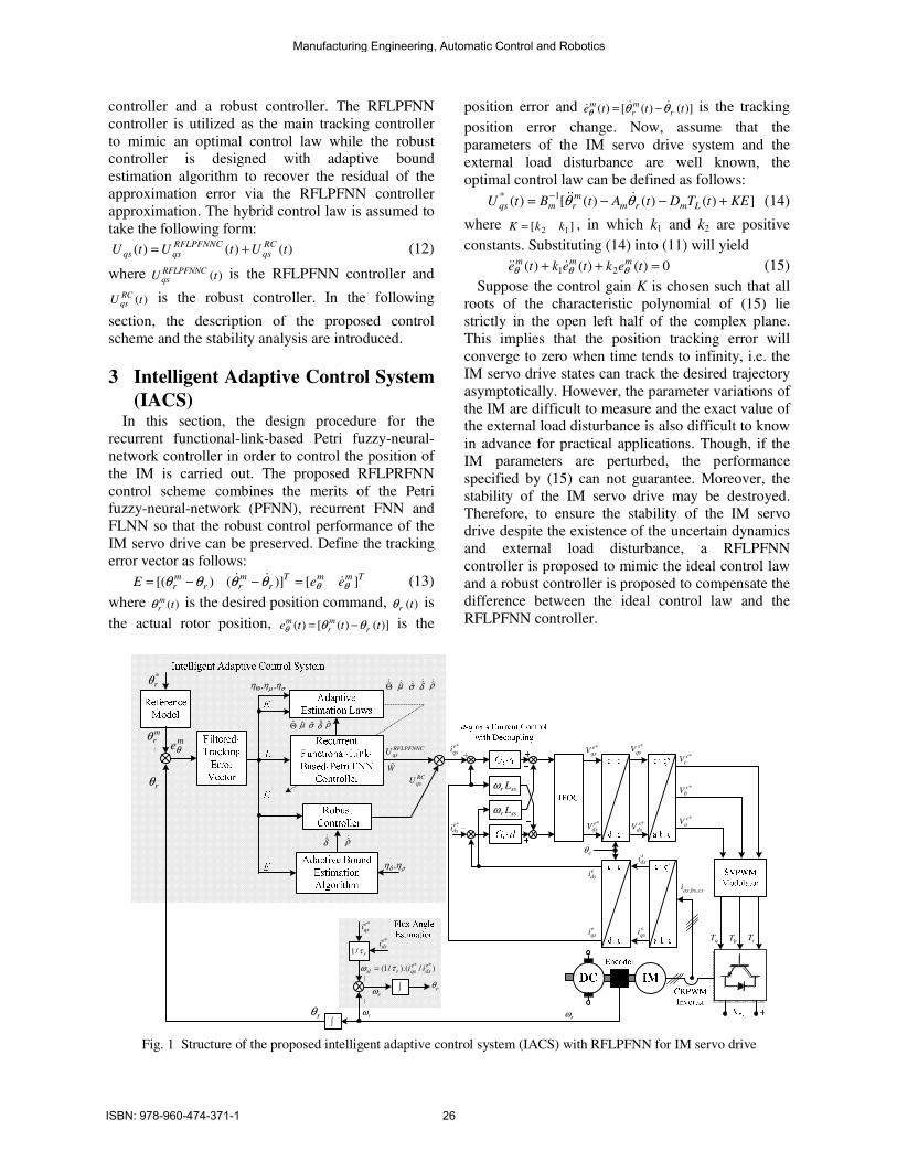
Abstract: This paper presents an intelligent adaptive control system (IACS) using a recurrent functional-link-
based Petri fuzzy-neural-network (RFLPFNN) for induction motor (IM) servo drive to achieve high dynamic
performance. The proposed IACS comprises a RFLPFNN controller and a robust controller. The RFLPFNN
controller is used as the main tracking controller to mimic an optimal control law while the robust controller is proposed to compensate the difference between the optimal control law and the RFLPFNN controller. Moreover,
the structure and parameter-learning of the RFLPFNN are performed concurrently. Furthermore, an on-line
parameter training methodology, which is derived based on the Lyapunov stability analysis and the back
propagation method, is proposed to guarantee the asymptotic stability of the IACS for the IM servo drive. In
addition, to relax the requirement for the bound of minimum approximation error and Taylor higher-order terms,
an adaptive control law is utilized to estimate the mentioned bounds. A computer simulation is developed and an
experimental system is established to validate the effectiveness of the proposed IACS. All control algorithms are implemented in a TMS320C31 DSP-based control computer. The simulation and experimental results
confirm that the IACS grants robust performance and precise response regardless of load disturbances and IM
parameters uncertainties.
Key-Words: Functional-link neural-networks (FLNNs), intelligent control, indirect field-orientation control
(IFOC), induction motor, Lyapunov satiability theorem, Petri net (PN), fuzzy-neural-network, robust control.
1 Introduction Induction motors (IMs) have many advantageous
characteristics such as high robustness, reliability
and low cost compared with DC motors. In the last
two decades, field-oriented control has become the
preferred method used in the control of high
performance IM drives. The objective is to obtain a
torque dynamic similar to that of a separately excited DC motor. Therefore, IM drives are frequently used
in high-performance industrial applications which
require independent torque and speed/position
control. Induction motors also possess complex
nonlinear, time-varying and temperature dependency
mathematical model. However, the control
performance of the IM drives is sensitive to the motor parameter variations, especially the rotor time
constant, which varies with the temperature and the
saturation of the magnetizing inductance. In addition,
the performance of IM drives is still influenced by
uncertainties, such as mechanical parameter variation,
external disturbance, unstructured uncertainty due to
non ideal field orientation in the transient state and
unmodeled dynamics. From a practical point of view,
complete information about uncertainties is difficult
to acquire in advance [1]-[2]. Therefore, in recent
years much research has been done to apply various
approaches to attenuate the effect of nonlinearities
and uncertainties of IM servo drives to enhance the
control performance [8]-[30]. Conventional
proportional-integral-derivative (PID) controllers are
widely used in industry due to their simple control
structure, ease of design and implementation [3]-[7].
However, the PID controller cannot provide robust
control performance because the IM servo drive system is highly nonlinear and uncertain. In addition,
an objection to the real-time use of such control
scheme is the lack of knowledge of uncertainties.
Due to the existence of nonlinearities, uncertainties,
and disturbances, conventional PID controller cannot
guarantee a sufficiently high performance for the IM
servo drive system. To deal with these uncertainties and nonlinearities and to enhance the control
Manufacturing Engineering, Automatic Control and Robotics
ISBN: 978-960-474-371-1 23
performance, many control techniques have been
developed for IM drive system, such as robust
control [8]-[11], sliding mode control (SMC) [12]-[16], intelligent control [17]-[24], hybrid control
[25]-[28], H∞ Control [29], [30]. These approaches
improve the control performance of the IM drive
from different aspects. Therefore, the motivation of
this paper is to design and implement a suitable
control scheme to confront the uncertainties existing
in practical applications of an indirect field-oriented
controlled IM drive.
The concept of incorporating fuzzy logic into a
neural network (NN) has grown into a popular
research topic. In contrast to the pure neural network
or fuzzy system, the fuzzy-neural-network (FNN)
possesses both their advantages; it combines the
capability of fuzzy reasoning in handling uncertain
information and the capability of NNs in learning
from the process [31]-[35]. On the other hand, the
recurrent fuzzy-neural-network (RFNN), which
naturally involves dynamic elements in the form of feedback connections used as internal memories, has
been studied in the past few years [34], [35]. In
recent years, Petri net has found widely applications
in modeling and controlling discrete event dynamic
systems [36]-[39]. For the last decades, Petri net
(PN) has developed into a powerful tool for
modeling, analysis, control, optimization, and
implementation of various engineering systems [40]-
[46]. In [45], the concept of incorporating PN into a
traditional FNN to form a new type Petri FNN
(PFNN) framework for the motion control of linear
induction motor drive is presented. In [46], the
designed of a network structure by introducing PN
into RFNN to form a dynamic Petri RFNN
(DPRFNN) scheme for the path-tracking control of a
nonholomonic mobile robot is presented.
One of the important points in the design of FNNs
is the consequent part, which is able to impact
performance on using different types. Two types of
FNNs are the Mamdani-type and the Takagi-Sugeno-
Kang (TSK)-type. For Mamdani-type FNNs, the
minimum fuzzy implication is adopted in fuzzy
reasoning. For TSK-type FNNs, the consequence
part of each rule is a linear combination of input
variables. It has shown that TSK-type FNN offer
better network size and learning accuracy than Mamdani-type FNNs. In the TSK-type FNN, which
is a linear polynomial of input variables, the model
output is approximated locally by the rule
hyperplanes. Nevertheless, the traditional TSK-type
FNN does not take full advantage of the mapping
capabilities that may be offered by the consequent
part. Therefore, several researches [47]–[51]
considers trigonometric functions to replace the
traditional TSK-type fuzzy reasoning and also obtain
better performance. In this view, the functional-link
neural network (FLNN) has been proposed using trigonometric functions to construct the consequent
part. The functional expansion increases the
dimensionality of the input vector and thus creation
of nonlinear decision boundaries in the
multidimensional space and identification of
complex nonlinear function become simple with this
network. It seems to be more efficient to include the functional-link fuzzy rules into the PFNN. In [48]-
[50], a functional-link-based fuzzy neural network
for nonlinear system control is proposed., which
combines a fuzzy neural network with FLNN. The
consequent part of the fuzzy rules that corresponds to
an FLNN comprises the functional expansion of the
input variables.
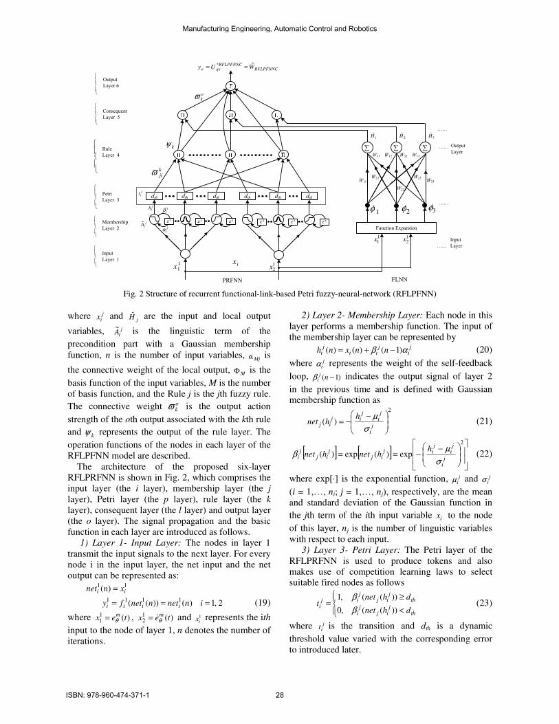
With the above mention motivations, this paper
presents the combination of PFNN and a FLNN to
construct the consequent part, called recurrent
FLNN-based PFNN (RFLPFNN) controller, for
dynamic system identification and control of IM
servo drive system. The proposed RFLPFNN is designed to improve the accuracy of functional
approximation. Each fuzzy rule that corresponds to
an FLNN consists of a functional expansion of input
variables. The orthogonal polynomials and linearly
independent functions are adopted as FLNN bases.
An online learning algorithm, consisting of structure
learning and parameter learning, is proposed to construct the RFLPFNN model automatically. The
structure learning algorithm determines whether or
not to add a new node that satisfies the fuzzy
partition of input variables. Initially, the RFLPFNN
model has no rules. The rules are automatically
generated from training data by entropy measure.
The parameter learning algorithm is based on back propagation to tune the parameters in the RFLPFNN
model simultaneously to minimize an output error
function. The advantages of the proposed RFLPFNN
model are summarized as follows. First, the
consequent of the fuzzy rules of the proposed
RFLPFNN is a nonlinear combination of input
variables. This paper uses the FLNN to the
consequent part of the fuzzy rules. The functional
expansion in RFLPFNN can yield the consequent
part of a nonlinear combination of input variables to
be approximated more effectively. Second, the
online learning algorithm can automatically construct
the RFLPFNN. No rules or memberships exist initially. They are created automatically as learning
proceeds, as online incoming training data are
received and as structure and parameter learning are
performed. Third, as demonstrated in Section 3, the
proposed RFLPFNN can solve temporal problems
Manufacturing Engineering, Automatic Control and Robotics
ISBN: 978-960-474-371-1 24
effectively and is a more adaptive and efficient
controller than the other methods.
This paper is organized as follows. Section 2 presents the indirect field-orientation control and
dynamic analysis of the IM servo drive as well as the
problem formulation. Section 3 presents the
description of the intelligent adaptive control system
for the IM servo drive. In addition, the design
procedures and adaptive learning algorithms of the
proposed RFLPFNN control system and the robust controller are described in details in Section 3. As
well, the stability analysis of the proposed control
system is introduced. The validity of the design
procedure and the robustness of the proposed
controller are verified by means of computer
simulation and experimental analysis. All control
algorithms have been developed in a control
computer that is based on a TMS320C31 and
TMS320P14 DSP DS1102 board. The dynamic
performance of the IM drive system has been studied
under load changes and parameter uncertainties.
Numerical simulations and experimental results are
provided to validate the effectiveness of the proposed control system in Section 4. Conclusions are
introduced in Section 5.
2 Preliminaries
2.1 Induction Motor Dynamic Model and
Indirect Field-Orientation Control
The dynamic model of the three-phase squirrel-cage
Y-connected IM in d-q axis arbitrary reference frame
is helpful to analyze all its characteristics for
dynamic analysis and control [1], [2]. The voltage
equation of the d-q model based on the stator
currents and rotor fluxes is given by (1) and the
electromagnetic torque is given by (2) while the
mechanical equation of the IM is given by (3).
The electromagnetic torque can be expressed as:
⋅
+−−−
−+−
−+−
+
=
dr
qr
ds
qs
r
r
r
m
r
rr
m
r
m
r
msss
r
m
r
msss
dr
qr
ds
qs
i
i
dt
dL
dt
dL
dt
d
L
L
L
L
dt
dLRL
L
L
dt
d
L
LL
dt
dLR
V
V
V
V
λ
λ
τωω
τ
ωωττ
ωσσω
ωσωσ
1)(0
)(1
0
(1)
( )dsqrqsdrr
mme ii
L
LPT λλ −=
22
3 (2)
The mechanical equation can be expressed as:
Lrm
mrm
me Tdt
d
Pdt
d
PJT +
+
= θβθ
222
2
(3)
The IFOC dynamics for the IM is derived from (1)
and (2) respectively at the synchronous reference
frame by setting 0=eqrλ 0/ =dtd
eqrλ and eωω = . The
torque equation and slip angular frequency for rotor
flux orientation are given in (4) and (5) while the
voltage commands are given in (6)-(9) [2].
**2
22
3 eqs
eds
r
mme ii
L
LPT = (4)
*
*1
eds
eqs
rsl
i
i
τω = (5)
( )****
eqss
eqss
eqs
eqs iRpiLeV +=− σ (6)
( ) *2* . ./ edserms
eqs iLLLe ωσ += (7)
( )**** edss
edss
eds
eds iRpiLeV +=+ σ (8)
( ) *2* . ./ eqserms
eds iLLLe ωσ += (9)
where Vqs, Vds, iqs and ids are the d-q axis stator
voltages and d-q axis stator currents, λqr and λdr are
the q-axis rotor flux and d-axis rotor flux,
respectively. Rs, Rr, Ls, Lr and Lm are the stator
resistance, rotor resistance, stator self inductance,
rotor self inductance and mutual inductance,
respectively. ωr, θr, J and β are the rotor speed, the
rotor position, the effective inertia and the friction
coefficient, respectively. Te, TL, τr, τs and ωsl are the
electromagnetic torque, the load torque, the rotor
time constant, the stator time constant and the slip
angular frequency, respectively. eqs, eds, ω and ωe are
the back emfs, the angular frequency of the arbitrary
and the synchronous reference frames respectively. σ
and Pm are the leakage flux coefficient and the
number of poles, respectively. rrr RL /=τ and
rsmrs LLLLL /)( 2−=σ . The parameters of the IM are
listed in Table (1).
The dynamic analysis of the IM may be expressed
as follows. From (3) and (4), the mechanical
dynamics can be simplified as:
Lmm
eqs
mm
tr
mm
mr T
JPi
PJ
K
PJ
1222 * −+−= θβ
θ &&& (10)
Lmmrmr TDtUBA ++= )(θθ &&& (11)
where )()( *titU
eqs= is the control effort,
*2 )/)(2/)(2/3( edsrmmt iLLPK = , )2/)(/( mmmm PJA β−= ,
)2/)(/( mmtm PJKB = and )/1)(2/( mmm JPD −= .
2.2 Problem Formulation
In order to efficiently control the rotor position of the
IM drive system, an IACS is proposed to increase the
robustness of the IFOC-IM drive system. The
intelligent adaptive control system for the IM drive is
shown in Fig. 1, in which the reference model is used
as the closed loop transfer function of the drive
system with the 2DOF I-PD position controller [20].
The proposed controller combines a RFLPFNN
Manufacturing Engineering, Automatic Control and Robotics
ISBN: 978-960-474-371-1 25
controller and a robust controller. The RFLPFNN
controller is utilized as the main tracking controller
to mimic an optimal control law while the robust controller is designed with adaptive bound
estimation algorithm to recover the residual of the
approximation error via the RFLPFNN controller
approximation. The hybrid control law is assumed to
take the following form:
)()()( tUtUtURCqs
RFLPFNNCqsqs += (12)
where )(tURFLPFNNCqs
is the RFLPFNN controller and
)(tURCqs
is the robust controller. In the following
section, the description of the proposed control
scheme and the stability analysis are introduced.
3 Intelligent Adaptive Control System
(IACS) In this section, the design procedure for the
recurrent functional-link-based Petri fuzzy-neural-
network controller in order to control the position of
the IM is carried out. The proposed RFLPRFNN
control scheme combines the merits of the Petri fuzzy-neural-network (PFNN), recurrent FNN and
FLNN so that the robust control performance of the
IM servo drive can be preserved. Define the tracking
error vector as follows: TmmT
rmrr
mr eeE ][)]()([ θθθθθθ &&& =−−= (13)
where )(tmrθ is the desired position command, )(trθ is
the actual rotor position, )]()([)( ttte rmr
m θθθ −= is the
position error and )]()([)( ttte rmr
m θθθ&&& −= is the tracking
position error change. Now, assume that the
parameters of the IM servo drive system and the
external load disturbance are well known, the
optimal control law can be defined as follows:
])()()([)(1*
KEtTDtAtBtU Lmrmmrmqs +−−= − θθ &&& (14)
where ][ 12 kkK = , in which k1 and k2 are positive
constants. Substituting (14) into (11) will yield
0)()()( 21 =++ tektekte mmmθθθ &&& (15)
Suppose the control gain K is chosen such that all
roots of the characteristic polynomial of (15) lie
strictly in the open left half of the complex plane.
This implies that the position tracking error will
converge to zero when time tends to infinity, i.e. the
IM servo drive states can track the desired trajectory
asymptotically. However, the parameter variations of
the IM are difficult to measure and the exact value of the external load disturbance is also difficult to know
in advance for practical applications. Though, if the
IM parameters are perturbed, the performance
specified by (15) can not guarantee. Moreover, the
stability of the IM servo drive may be destroyed.
Therefore, to ensure the stability of the IM servo
drive despite the existence of the uncertain dynamics
and external load disturbance, a RFLPFNN
controller is proposed to mimic the ideal control law
and a robust controller is proposed to compensate the
difference between the ideal control law and the
RFLPFNN controller.
*rθ
mrθ
rθ
meθ
rθ
RFLPFNNCqsU
σµ ηηη ,,Θ
WRCqsU
σ&Θ& µ&
ρδ ηη ,
*sdsV
*sqsV
*ccV
*cbV
*caV
csbsasi ,,
sdsi
sqsi
eθ
aTbT cT
ssr Lω
ssr Lω
∫
σΘ µ
rω
*eqsi
*edsi
*eqsV
*edsV
edsi
eqsi
rω
)/).(/1( ** eds
eqsrsl iiτω =
rτ/1
eω
*eqsi
*edsi
∫ eθ
δ& ρ&
δ ρ
δ& ρ&
Fig. 1 Structure of the proposed intelligent adaptive control system (IACS) with RFLPFNN for IM servo drive
Manufacturing Engineering, Automatic Control and Robotics
ISBN: 978-960-474-371-1 26
Table (1) Parameters of IM
Quantity Symbol Value Nominal power Pn 1.5 kW (3-phase)
Rated voltage VL-L 380 V
Nominal speed (electrical) ωr 296.48 rad/sec
Nominal speed (mechanical) Nr 1415 rpm
Number of poles Pm 4
Rated torque Te 12 N.m
Rated current I 3.8 A
Rated frequency f 50 Hz
Self inductance Ls = Lr 480 mH
Magnetizing inductance Lm 464 mH
Stator winding resistance Rs 6.30 Ω
Rotor resistance Rr 3.60 Ω
Rotor inertia Jm 0.038 kg.m2
Friction coefficient βm 0.0085
N.m/rad/sec
Resolution of the encoder nE 5000 p/r
The control performance of the IM drives is
sensitive to the parameter variations, external
disturbance, unstructured uncertainty and unmodeled
dynamics. Especially the rotor time constant, this varies with the temperature and the saturation of the
magnetizing inductance. Therefore, conventional
PID controller cannot guarantee a sufficiently high
performance for the IM servo drive. To deal with
these uncertainties and nonlinearities and to enhance
the control performance, the IACS with RFLPFNN
has been proposed for IM servo drive system.
The following subsections describe the structure of
FLNNs and RFLPFNN models. The RFLPFNN
adopted the FLNN and generating complex nonlinear
combinations of input variables to the consequent
part of the fuzzy rules. The details of these structures
are given below.
3.1 Functional-Link Neural-Network (FLNN)
To improve the accuracy of the function
approximation, an FLNN is adopted to implement
the function expansion for the proposed RFLPFNN.
The architecture of the FLNN is shown in Fig. 2, in
which the functional link acts on an element of input
variables by generating a set of linearly independent
functions, i.e., function expansion. In the function
expansion of the FLNN, basis functions such as
trigonometric, Gaussian, or other orthogonal
polynomials are feasible. In this paper, the
trigonometric function is adopted since it forms a
more compact representation than the Gaussian basis,
and the sine and cosine functions can be computed
more quickly. Moreover, better performance results
when the outer product term is taken into account in
the function expansion [47]. Therefore, for a two-
dimensional input vector Txx ],[ 21=Χ , the input
variables are obtained using trigonometric functions
and can be separated in the enhanced space
==Φ TM ],,,[ 21 φφφ K ),sin( , ),cos( ),sin( , ,1[ 22111 xxxxx πππ
Txxxx ] ),cos( ),sin( 2122 ππ , where x1x2 is the outer
product term. In the FLNN structure shown in Fig. 2,
a set of basis functions Φ and a fixed numbers
weight parameters W represent fW(x). The theory
behind the FLNN for multidimensional function approximation has been discussed in [47], [51]. Let
M
kkB1== φ be a set of basis functions to be considered
as shown in Fig. 2. The FLNN comprises M basis
functions MM B∈φφφ ,,, 21 K . The output of the FLNN
is given by a linear sum of the jth node as
mjM
H
MMjjjj
MM
Mjj
,,1 and 8,2,1 ,
)(ˆ
332211
LL
L
==
++++=
ΧΦ∑=
φωφωφωφω
ω
(16)
where nℜ∈Χ , Tnxxx ],,,[ 21 K=Χ is the input vector
and TMjjjjW ],,,[ 21 ωωω K= is the weight vector
associated with the jth output of the FLNN. jH
denotes the local output of the FLNN structure and
the consequent part of the jth fuzzy rule in the
RFLPFNN. Therefore, the matrix form of (16) can
be expressed as
Φ= jj WH (17)
where Tn xxx )](,),(),([ 21 φφφ K=Φ is the basis function
vector which is the output of the functional
expansion block. In the RFLPFNN, the corresponding weights of functional link bases do
not exist in the initial state, and the amount of the
corresponding weights of functional link bases
generated by the online learning algorithm is
consistent with the number of fuzzy rules.
3.2 Structure of Recurrent Functional-Link-
Based Petri Fuzzy-Neural-Network This subsection describes the RFLPFNN, which uses
a nonlinear combination of input variables (FLNN).
Each fuzzy rule corresponds to a sub-FLNN,
comprising a functional link. Fig. 2 represents the
structure of the proposed RFLPFNN.
The RFLPFNN model realizes a fuzzy IF-THEN
rule in the following form:
Rule j:
IF 11x is j
A1
~ and 1
2x is jA2
~ ... and j
ix is jiA
~... and j
nx
is jnA
~ THEN
MMjjjj
MM
MjjH
φωφωφωφω
ω
++++=
ΧΦ∑=
L332211
)(ˆ
MM
Mj
N
kk
oko
r
y Φ∑∑==
ωψϖ ..1
(18)
Manufacturing Engineering, Automatic Control and Robotics
ISBN: 978-960-474-371-1 27
11x 1
2x
RFLPFNNCRFLPFNNC
qso WUy ˆ* ==
11x 1
2x
jiA
~j
iA~
kjiϖ
ix
Membership
Layer 2
Output
Layer 6
Input
Layer 1
Petri
Layer 3
Rule
Layer 4
Consequent
Layer 5
Input
Layer
Output
Layer∑ ∑∑
1H 3H2H
1φ
Function Expansion
W11
W12 W13
W21
W22
W23W33
W31 W32
LL
LL
LL
LL
2φ 3φ
z-1 z-1 z-1z-1 z-1 z-1
dthdthdth dth dth dth
jit
jih j
iβ
jiα
okϖ
kψ
FLNNPRFNN
Fig. 2 Structure of recurrent functional-link-based Petri fuzzy-neural-network (RFLPFNN)
where jix and
jH are the input and local output
variables, jiA
~ is the linguistic term of the
precondition part with a Gaussian membership
function, n is the number of input variables, Mjω is
the connective weight of the local output, MΦ is the
basis function of the input variables, M is the number
of basis function, and the Rule j is the jth fuzzy rule.
The connective weight okϖ is the output action
strength of the oth output associated with the kth rule
and kψ represents the output of the rule layer. The
operation functions of the nodes in each layer of the
RFLPFNN model are described.
The architecture of the proposed six-layer
RFLPRFNN is shown in Fig. 2, which comprises the
input layer (the i layer), membership layer (the j
layer), Petri layer (the p layer), rule layer (the k
layer), consequent layer (the l layer) and output layer
(the o layer). The signal propagation and the basic
function in each layer are introduced as follows.
1) Layer 1- Input Layer: The nodes in layer 1
transmit the input signals to the next layer. For every
node i in the input layer, the net input and the net
output can be represented as: 11
)( ii xnnet =
2 ,1)())(( 1111 === innetnnetfy iiii (19)
where )(11 tex m
θ= , )(12 tex m
θ&= and 1ix represents the ith
input to the node of layer 1, n denotes the number of
iterations.
2) Layer 2- Membership Layer: Each node in this
layer performs a membership function. The input of
the membership layer can be represented by j
ij
iij
i nnxnh αβ )1()()( −+= (20)
where jiα represents the weight of the self-feedback
loop, )1( −nj
iβ indicates the output signal of layer 2
in the previous time and is defined with Gaussian membership function as
2
)(
−−=
ji
ji
jij
ij
hhnet
σ
µ (21)
[ ] [ ]
−−==
2
exp)(exp)(j
i
ji
jij
ijj
ijj
i
hhnethnet
σ
µβ (22)
where exp[⋅] is the exponential function, jiµ and j
iσ
(i = 1,…, ni; j = 1,…, nj), respectively, are the mean
and standard deviation of the Gaussian function in
the jth term of the ith input variable ix to the node
of this layer, nj is the number of linguistic variables
with respect to each input.
3) Layer 3- Petri Layer: The Petri layer of the
RFLPRFNN is used to produce tokens and also
makes use of competition learning laws to select suitable fired nodes as follows
<
≥=
thj
ijj
i
thj
ijj
iji
dhnet
dhnett
))((,0
))((,1
β
β (23)
where jit is the transition and dth is a dynamic
threshold value varied with the corresponding error
to introduced later.
Manufacturing Engineering, Automatic Control and Robotics
ISBN: 978-960-474-371-1 28
4) Layer 4- Rule Layer: Each node k in layer 4
(rule layer) is denoted by ∏, which multiplies the
incoming signals and outputs the result of the
product. For the kth nodes:
=
=∏= =
0,0
1)),((1
ji
ji
n
i
jij
ji
kji
k
t
thnetnet
βϖ (24)
From (22) and (24), we can obtain
r
ji
ji
n
ij
i
ji
jik
jikkk
Nk
t
th
netf
,,1
0,0
1,exp)( 1
2
K=
=
=∏
−−
== = σ
µϖ
ψ(25)
where jiβ represents the jth input to the node of the
rule layer, kψ represents the kth output of the rule
layer; kjiϖ , the connective weights between the Petri
layer and the rule layer. These weights are assumed
to be unity; and Nr is the total number of rules.
5) Layer 5-Consequent Layer: Nodes in this layer
are called consequent nodes. The input to a node in
layer 5 is the output from layer 4 and the other inputs
are nonlinear combinations of input variables from
the FLNN jH as shown in Fig. 2. For such node
=
=∏Φ∑=
Φ∑==
=
0,0
1)),((.
.ˆ.
1j
i
ji
n
i
jij
ji
kjiM
MMj
MM
Mjkjklj
t
thnet
Hy
βϖω
ωψψ
(26)
where Mjω is the corresponding connective weight of
the FLNN and MΦ is the functional expansion of
input variables. The functional expansion uses a
trigonometric polynomial basis function, given by
)]cos()sin()cos()sin([ 222111 xxxxxx ππππ for two-
dimensional input variables. Moreover, the output
nodes of the FLNN depend on the number of fuzzy
rules of the RFLPFNN model.
6) Layer 6- Output Layer: Each node in this layer
corresponds to a single output variable. The output
node in layer 6 integrates all of the actions from
layer 4 and 5 and acts as a center of area defuzzifier.
MM
Mj
N
kk
oko
r
net Φ∑∑==
ωψϖ ..1
(27)
1 )( === onetnetfy oooo (28)
∑
Φ∑∑=
∑
∑=
=
=
=
=
r
r
r
r
N
kk
ok
MM
Mj
N
kk
ok
N
kk
ok
N
kk
okj
o
H
y
1
1
1
1
.
..
.
..ˆ
ψϖ
ωψϖ
ψϖ
ψϖ (29)
where the connective weight okϖ is the output action
strength of the oth output and oy is the output of the
RFLPFNN and Nr is the total number of rules.
The output of the RFLPFNN controller,
)(tUyRFLPFNNCqso = , can be rewritten as
ΩΘ=Θ= TRFLPFNNC
RFLPFNNCqs EWU ),,,( σµ (30)
where the tracking error vector E is the input of the
RFLPFNN, Θ are the collections of the adjustable
parameters ),,( ok
jiMj ϖαω , Ω is the output vector
),( Mk Φψ and TmmeeE ][ θθ &= is the tracking error input
vector to the RFLPFNN controller.
3.3 Learning Algorithms of the Recurrent
FLNN-based PFNN Model This section presents the online learning algorithm
for constructing the recurrent FLNN-based PFNN
model. The proposed learning algorithm comprises
structure learning and a parameter learning
algorithms. Structure learning is based on the
entropy measure used to determine whether a new
rule should be added to satisfy the fuzzy partitioning of input variables [52]. Parameter learning is based
on supervised learning algorithms. The
backpropagation algorithm minimizes a given cost
function by adjusting the link weights in the
consequent part and the parameters of the
membership functions [46]. Initially, there are no
nodes in the network except the input-output nodes, i.e., there are no nodes in the RFLPFNN model. The
nodes are created automatically as learning proceeds,
upon the reception of online incoming training data
in the structure and parameter learning processes.
3.4 Robust Control Design and Stability
Analysis of the IACS In this section, the intelligent adaptive control system
is proposed to mimic the optimal control law defined
in (14) using RFLPFNN controller and the robust
controller is designed with adaptive bound
estimation algorithm to compensate the difference between the optimal control law and the output of the
RFLPRFNN controller. The proposed controller
combines the merits of the PFNN [45], recurrent
neural network and FLNN. The design of robust
controller is necessary to compensate the minimum
approximation error instead of increasing the rules of
the RFLPFNN controller. From (11), (12) and (14), an error equation is obtained as follows:
( )RCqs
RFLPFNNCqsqsm UUUBEE −−+Λ= ˆ*& (31)
where
−−=Λ
12
10
kk is a stable matrix and
Tmm BB ]0[= . To develop the robust controller, a
minimum approximation error ε is defined as:
),,,(***** σµε Θ−= EUU
RFLPFNNCqsqs (32)
Manufacturing Engineering, Automatic Control and Robotics
ISBN: 978-960-474-371-1 29
where *Θ is the optimal weight vector achieves the
minimum approximation error and ε is the
approximation error and is assumed to be bounded
by δε < . *Θ , *µ and *σ are the optimal parameters
of Θ , µ and σ in the RFLPFNNC. From (32), the
error equation in (31) can be rewritten as:
( )
( )( )RC
qsTT
m
RCqsqsm
RCqs
RFLPFNNCqs
RFLPFNNCqs
RFLPFNNCqsqsm
RCqs
RFLPFNNCqsqsm
UBE
UUBE
UUU
UUBE
UUUBEE
−ΩΘ+ΩΘ++Λ=
−++Λ=
−−+
−+Λ=
−−+Λ=
~ˆ~
~
]ˆ[
][
ˆ
*
*
**
*
ε
ε
&
(33)
where )ˆ(~ * Θ−Θ=Θ and )ˆ(
~ * Ω−Ω=Ω . The weights
of the RFLPFNNC are updated online to guarantee
the closed-loop stability and perfect tracking
performance. To achieve this goal, the linearization
technique is used to transform the nonlinear output
of PRFLPFNNC into partially linear form so that the
Lyapunov theorem extension can be applied. The
expansion of Ω~
in Taylor series is obtained as:
UTT
U
T
j
T
jj
O
O
+Ω+Ω≡
+
∂
Ω∂
∂
Ω∂
∂
Ω∂
+
∂
Ω∂
∂
Ω∂
∂
Ω∂
=
Ω
Ω
Ω
=Ω
==
σµ
σ
σ
σ
σ
µ
µ
µ
µ
σµ
σσµµ
~~
~~
~
~
~
~
ˆ
2
1
ˆ
2
1
2
1
MMM (34)
where [ ]µµ
µ µµµˆ
21 )/()/()/(=
∂Ω∂∂Ω∂∂Ω∂=ΩT
jL ,
[ ]σσ
σ σσσˆ
21 )/()/()/(=
∂Ω∂∂Ω∂∂Ω∂=Ω TjL ,
)ˆ(~ * µµµ −= , )ˆ(~ * σσσ −= and OU is a vector of
higher order terms and assumed to be pounded by a
positive constant. Rewriting (34), it can be obtained that
UTT
O+Ω+Ω+Ω=Ω σµ σµ~~ˆ* (35)
Assume that
)ˆ(~ *
qsqsqs UUU −= (36)
From (35) and (36), we can obtain
Γ+ΩΘ+ΩΘ+ΩΘ=
ΩΘ−+Ω+Ω+ΩΘ=
ΩΘ−ΩΘ=−=
σµ
σµ
σµ
σµ
~ˆ~ˆˆ~
ˆˆ]~~ˆ[
ˆˆ)ˆ(~
*
***
TTTTT
TQ
TTT
TTqsqsqs
O
UUU
(37)
where the uncertain term
UTTTTT O*~~~~
Θ+ΩΘ+ΩΘ=Γ σµ σµ is assumed to be
bounded (i.e. ρ<Γ ). According to (33) and (35)-(37),
the error dynamics can be represented as
( ))~ˆ~ˆˆ~
(
~
RCqs
TTTTTm
RCqsqsm
UBE
UUBEE
−Γ++ΩΘ+ΩΘ+ΩΘ+Λ=
−++Λ=
εσµ
ε
σµ
&
(38)
Theorem: Consider the IM servo drive system
represented by (11), if the intelligent controller is
designed as (12), in which the adaptation laws of the
RFLPFNN controller are designed as (39)-(41) and
the robust controller is designed as (42) with the
adaptive bound estimation algorithms given in (43)
and (44). As a result, the stability of the intelligent
adaptive control system can be guaranteed.
Tm
TPBE Ω=Θ Θ
ˆˆ η&
(39)
TTm
T PBE µµηµ ΩΘ= ˆˆ& (40)
TTm
T PBE σσησ ΩΘ= ˆˆ& (41)
)sgn()ˆˆ( mTRC
qs PBEU ρδ += (42)
mT
PBEt δηδ =)(&
(43)
mT
PBEt ρηρ =)(& (44)
where ηΘ, ηµ, ησ, ηδ and ηρ are strictly positive
learning rates, )sgn(⋅ is the sign function, )(ˆ tδ and
)(ˆ tρ are the on-line estimated values of the adaptive
bounds )(tδ and )(tρ .
Proof: To minimize the error function and to
derive the adaptation laws of Θ , µ , σ , δ and ρ
for the intelligent adaptive control system, a
Lyapunov function is defined as:
22 ~
2
1~
2
1~~
2
1
~~
2
1~~
2
1
2
1
),~,~
,~,~,~
,(
ρη
δη
σση
µµηη
ρδσµ
ρδσ
µ
+++
+ΘΘ+=
Θ
Θ
T
TTT PEE
tEV
(45)
where )ˆ(~
δδδ −= and )ˆ(~ ρρρ −= are the estimated
errors and nnP
×ℜ∈ is a symmetric positive-definite
matrix, which satisfies the following Lyapunov equation [53], [54].
QPPT −=Λ+Λ (46)
where nnQ
×ℜ∈ is a given symmetric positive definite
matrix, 0>Q . By taking the derivative of the
Lyapunov function (45) and using (38) and (46), it is
obtained that:
ρρη
δδη
σση
µµηη
ρδσµ
ρδσ
µ
&&&
&&&&
&
~~1~~1~~1
~~1~~1
2
1
2
1
),~,~
,~,~,~
,(
+++
+ΘΘ++=
Θ
Θ
T
TTTTPEEEPE
tEV
(47)
Substitute (38)-(44) into (47), then
Manufacturing Engineering, Automatic Control and Robotics
ISBN: 978-960-474-371-1 30
02
1
)()(2
1
)ˆ()ˆ(
)ˆˆ(2
1
)~~()(2
1
ˆ~1ˆ~1ˆ~1
ˆ~1ˆ~1)~ˆ
~ˆˆ~(
2
1
ˆ~1ˆ~1ˆ~1
ˆ~1ˆ~1)~ˆ
~ˆˆ~(
2
1
2
1
ˆ~1ˆ~1ˆ~1
ˆ~1ˆ~1
2
1
2
1
),~,~
,~,~,~
,(
*
≤−≤
−Γ+−+−=
−+−+
+−Γ++−=
+−−Γ++−=
−−−
−ΘΘ−−Γ++ΩΘ+
ΩΘ+ΩΘ+−=
−−−
−ΘΘ−−Γ++ΩΘ+
ΩΘ+ΩΘ+Λ+Λ=
−−−
−ΘΘ−+=
Θ
Θ
Θ
Θ
QEE
BPEBPEQEE
BPEBPE
PBEBPEBPEQEE
BPEUBPEQEE
U
BPEQEE
U
BPEPEEEPE
PEEEPE
tEV
T
mT
mTT
mT
mT
mT
mT
mTT
mTRC
qsmTT
T
TTRCqs
TT
TTTm
TT
T
TTRCqs
TT
TTTm
TTTT
T
TTTT
ρδε
ρρδδ
ρδε
ρσε
ρρη
δδη
σση
µµηη
εσ
µ
ρρη
δδη
σση
µµηη
εσ
µ
ρρη
δδη
σση
µµηη
ρδσµ
ρδσ
µσ
µ
ρδσ
µσ
µ
ρδσ
µ
&&&
&&
&&&
&&
&&&
&&&&
&
(48)
Since 0),~,~
,~,~,~
,( ≤Θ tEV ρδσµ& , ),~,~
,~,~,~
,( tEV ρδσµΘ&
is a negative semi-definite function (i.e.
≤Θ ),~,~
,~,~,~
,( tEV ρδσµ& )0,~,~
,~,~,~
,( ρδσµΘEV& ), which
implies that E, Θ~
, µ~ , σ~ , δ~
and ρ~ are bounded
function. Let the function
),~,~
,~,~,~
,()2/1()( tEVQEEtT ρδσµΘ−≤=Ξ & and integrate the
function )(tΞ with respect to time yields:
),~,~
,~,~,~
,(
)0,~,~
,~,~,~
,()(0
tEV
EVdt
ρδσµ
ρδσµττ
Θ−
Θ≤∫Ξ (49)
Since )0,~,~
,~,~,~
,( ρδσµΘEV is bounded and
),~,~
,~,~,~
,( tEV ρδσµΘ is non-increasing and bounded,
the following result can be obtained:
∞≤∫Ξ∞→
ττ dt
t 0
)(lim (50)
Differentiate )(tΞ with respect to time, then
EQEtT &=Ξ )( (51)
In addition, since all variables in the right hand
side of (32) are bounded, it implies E& is also
bounded, then )(tΞ& uniformly continuous [53]. By
using Barbalat’s Lemma [53], [54], it can be shown
that 0)(lim =Ξ∞→
tt
. That is, 0)( →tE as ∞→t . As a
result, the IACS is asymptotically stable. Moreover,
the tracking error of the system will converges to
zero according to 0)( =tE .
4 Numerical Simulation and
Experimental Results In order to investigate the effectiveness of the
proposed tracking control scheme, the simulation and
experimentation of the proposed IACS are carried
out using MATLAB/SIMULINK package based on
the control system shown in Figs. 1 and 3. The
simulation and experimental results of the IM servo
drive system are presented to verify the feasibility of
the proposed IACS under various operating
conditions. The threshold values, learning rates and
the gains of the proposed control scheme are given as
follows: D=0.35, dth=0.25, ηΘ=0.75, ηµ=0.004,
ησ=0.005 ηδ=0.003, ηρ=0.3 k1=55 and k2=75. All the
proposed threshold values, learning rates and control
gains in the IACS are chosen to achieve the superior
transient control performance in the simulation and
experimentation considering the limitation of control
effort, the requirement of stability and the possible
operating conditions. When the threshold value dth=0
is set, the performance of the PFNN control system
is the same as the one of the FNN control system because all the control rules in the network structure
are fired at this situation. Although the
computational time can be gradually decreased by
increasing the threshold value, the control
performance also deteriorates little by little.
Therefore, we have to compromise between the
control performance and computational complexity. The control performance in the dynamic threshold
value of the RFLPFNN can be approximately
determined as γ =0.35 and ξ=250.
4.1 Numerical Simulation of the IM Servo Drive
System All numerical simulations are carried out using
Matlab/Simulink package. The control objective is to
control the position of the IM servo drive system to
track the reference model trajectory. To investigate the effectiveness and robustness of the proposed
control system, four simulated conditions including
parameter uncertainties (PU) and external load
disturbance are considered. The mechanical time
constant of the IM is given by )/( mmm Jβτ = .
Case 1: 1.0×τr, 1.0×τm, TL=0–12 N.m
Case 2: 0.5×τr, 0.5×τm, TL=0–12 N.m
Case 3: 1.5×τr, 2.5×τm, TL=0–12 N.m
Case 4: 1.5×τr, 5.0×τm, TL=0–12 N.m
The dynamic performance of the IM servo drive due
to reference model command under subsequent
loading of 12 N.m for the PFNN controller alone at
Case (1) of PU including the responses of the
reference model and rotor position, the tracking
Manufacturing Engineering, Automatic Control and Robotics
ISBN: 978-960-474-371-1 31
position error, rotor speed, the tracking speed error,
d-q axis current response and adaptive signals are
predicted in Fig. 4(a), respectively. On the other hand, the dynamic performance of the IM servo drive
using the IACS using RFLPFNN and robust
controllers is shown in Fig. 4(b) at Case (1) of PU.
The disturbance rejection capabilities have been
checked when a load of 12 N.m is applied to the
shaft at t = 2.5 sec and removed at t = 7.5 sec. The
results obtained in Fig. 4 illustrate good dynamic
performances, in command tracking and load
regulation performance, are realized for both position
tracking controllers. Improvement of the control performance by addition the proposed IACS can be
observed from the obtained results in command
tracking and load regulation characteristics. From
these results shown in Fig. 4, the tracking position
error and tracking speed error with the PFNN
controller is larger than the ones using the IACS.
(a) Experimental setup
(b) Block diagram of the proposed DSP-based control system
Fig. 3 DSP-based intelligent adaptive control system (IACS) using RFLPFNN for IM servo drive
Manufacturing Engineering, Automatic Control and Robotics
ISBN: 978-960-474-371-1 32
0 1 2 3 4 5 6 7 8 9 10-8
-4
0
4
8
Time (sec)
Ro
tor p
osi
tio
n (
ra
d)
Ref. Actual
0 1 2 3 4 5 6 7 8 9 10-0.6
-0.3
0
0.3
0.6
Time (sec)
Tra
ck
ing
Erro
r (
ra
d)
0 1 2 3 4 5 6 7 8 9 10-0.6
-0.3
0
0.3
0.6
Time (sec)
Tra
ck
ing
Erro
r (
ra
d)
0 1 2 3 4 5 6 7 8 9 10-8
-4
0
4
8
Time (sec)
Ro
tor P
osi
tio
n (
ra
d)
Ref. Actual
0 1 2 3 4 5 6 7 8 9 10-15
-7.5
0
7.5
15
Time (sec)
Ro
tor S
peed
(ra
d/s
ec)
Ref. Actual
0 1 2 3 4 5 6 7 8 9 10-6
-3
0
3
6
Time (sec)
Tra
ck
ing
Erro
r (
ra
d/s
ec)
0 1 2 3 4 5 6 7 8 9 10-15
-7.5
0
7.5
15
Time (sec)
Ro
tor S
peed
(ra
d/s
ec)
Ref. Actual
0 1 2 3 4 5 6 7 8 9 10-6
-3
0
3
6
Time (sec)T
ra
ck
ing
Erro
r (
ra
d/s
ec)
0 1 2 3 4 5 6 7 8 9 10-8
-4
0
4
8
Time (sec)
Iqse
-r (
A)
0 1 2 3 4 5 6 7 8 9 10-8
-4
0
4
8
Time (sec)
Iqse
-a (
A)
0 1 2 3 4 5 6 7 8 9 10-8
-4
0
4
8
Time (sec)
Iqse
-r (
A)
0 1 2 3 4 5 6 7 8 9 10-8
-4
0
4
8
Time (sec)
Iqse
-a (
A)
0 1 2 3 4 5 6 7 8 9 10-8
-4
0
4
8
Time (sec)
Idse
-r (
A)
0 1 2 3 4 5 6 7 8 9 10-8
-4
0
4
8
Time (sec)
Idse
-a (
A)
0 1 2 3 4 5 6 7 8 9 10-8
-4
0
4
8
Time (sec)
Idse
-r (
A)
0 1 2 3 4 5 6 7 8 9 10-8
-4
0
4
8
Time (sec)
Idse
-a (
A)
(a) (b)
Fig. 4 Dynamic response of the IM servo drive system for the reference position and subsequent loading of 12 N.m for
both position controllers at Case (1) of parameter uncertainties.
(a) Using PFNN tracking controller (b) Using IACS with RFLPFNN tracking controller
Manufacturing Engineering, Automatic Control and Robotics
ISBN: 978-960-474-371-1 33
0 1 2 3 4 5 6 7 8 9 10-8
-4
0
4
8
Time (sec)
Idq
ss-r
(A
)
0 1 2 3 4 5 6 7 8 9 10-8
-4
0
4
8
Time (sec)
Idq
ss-a
(A
)
0 1 2 3 4 5 6 7 8 9 10-8
-4
0
4
8
Time (sec)
Idq
ss-r
(A
)
0 1 2 3 4 5 6 7 8 9 10-8
-4
0
4
8
Time (sec)
Idq
ss-a
(A
)
0 1 2 3 4 5 6 7 8 9 10-5
-2.5
0
2.5
5
Time (sec)
Ad
ap
tiv
e S
ign
al
(ra
d)
0 1 2 3 4 5 6 7 8 9 10-20
-10
0
10
20
Time (sec)
Ad
ap
tiv
e s
ign
al
(ra
d/s
ec)
0 1 2 3 4 5 6 7 8 9 10-5
-2.5
0
2.5
5
Time (sec)
Ad
ap
tiv
e S
ign
al
(ra
d)
0 1 2 3 4 5 6 7 8 9 10-20
-10
0
10
20
Time (sec)A
da
pti
ve s
ign
al
(ra
d/s
ec)
(a) (b)
Fig. 4 (Continued) Dynamic response of the IM servo drive system for the reference position and subsequent loading of
12 N.m for both position controllers at Case (1) of parameter uncertainties.
(a) Using PFNN tracking controller (b) Using IACS with RFLPFNN tracking controller
To further verify the performance robustness of
the proposed control schemes, four cases of PU and
external load disturbance are considered, Cases
(1~4), for comparison. The dynamic performance of
the IM servo drive for both position controllers at all
Cases of PU is predicted in Fig. 5. From the
simulation results shown in Fig. 5(b), the tracking
errors converges quickly and the robust control
characteristics of the IM servo drive system using the
proposed IACS under the occurrence of PU can be
clearly observed. The proposed IACS provides a
rapid and accurate response for the reference model
under load changes within 0.5 sec compared with the PFNN position tracking controller which has
sluggish recovery time of more than 1.0 sec at PU as
shown in Fig. 5(a). Furthermore, the maximum
tracking position errors at four cases of PU are
approximately ±0.6 rad, for the PFNN controller. On
the other hand, the ones with the IACS at four
examined cases of PU are approximately constants
and equal ±0.25 rad. Comparing the IACS with the
PFNN controller, the tracking errors and regulation
characteristics using IACS are much reduced.
Therefore, the proposed IACS with RFLPFNN can
yield superior control performance than the PFNN
controller. As a result, the proposed IACS provides a
rapid and accurate response for the reference model
under load changes compared with the PFNN
position tracking controller which has sluggish
recovery time. Perfect tracking response and robust
characteristics can still be kept with regard to PU and
external disturbances as shown in Fig. 5(b). Thus, it
can be verified that the proposed IACS at all cases of
PU can satisfy the robustness, the accuracy
requirements and is more suitable in the tracking
control of the IM drive for industrial applications.
4.2 Experimentation of the IM Servo Drive
System The experimental setup for the IM servo drive
system is shown in Fig. 3. A DSP control board
dSPACE DS1102, which is based on a TMS320C31
and TMS320P14 DSPs, is installed in the control
computer which includes multi-channels of ADC, DAC, PIO and encoder interface circuits. Digital
filter and frequency multiplied by four circuits are
built into the encoder interface circuits to increase
the precision of the position feedback signal and
coordinate transformations. The sampling rate is
chosen as 200µs and hence, the carrier frequency of
the PWM inverter is 5 kHz. The control interval of
the position control loop is set at 1 ms. The current-
regulated PWM VSI is implemented using
MITSUBISHI intelligent power module (IPM) using
Manufacturing Engineering, Automatic Control and Robotics
ISBN: 978-960-474-371-1 34
IGBT components with a switching frequency of 15
kHz and driven by a six SEMIKRON IGBT drivers.
The DC-link LC filter components are an inductor of
iron powder core with 250µH and a polypropylene-
film capacitor with 5µF. The position acquisition has
been performed with a 5000 pulses/revolution
incremental optical encoder. Therefore, the output of
the frequency multiplier circuit is 4×5000
pulses/revolution which results high precision of the
speed/position measurement.
0 1 2 3 4 5 6 7 8 9 10-8
-4
0
4
8
Time (sec)
Ro
tor P
osi
tio
n (
ra
d)
0 1 2 3 4 5 6 7 8 9 10-0.6
-0.3
0
0.3
0.6
Time (sec)
Tra
ck
ing
Erro
r (
ra
d)
0 1 2 3 4 5 6 7 8 9 10-8
-4
0
4
8
Time (sec)
Ro
tor P
osi
tio
n (
ra
d)
0 1 2 3 4 5 6 7 8 9 10-0.6
-0.3
0
0.3
0.6
Time (sec)
Tra
ck
ing
Erro
r (
ra
d)
0 1 2 3 4 5 6 7 8 9 10-15
-7.5
0
7.5
15
Time (sec)
Ro
tor S
peed
(ra
d/s
ec)
0 1 2 3 4 5 6 7 8 9 10-6
-3
0
3
6
Time (sec)
Tra
ck
ing
Erro
r (
ra
d/s
ec)
0 1 2 3 4 5 6 7 8 9 10-15
-7.5
0
7.5
15
Time (sec)
Ro
tor S
peed
(ra
d/s
ec)
0 1 2 3 4 5 6 7 8 9 10-6
-3
0
3
6
Time (sec)
Tra
ck
ing
Erro
r (
ra
d/s
ec)
0 1 2 3 4 5 6 7 8 9 10-8
-4
0
4
8
Time (sec)
Iqse
-r (
A)
0 1 2 3 4 5 6 7 8 9 10-4
-2
0
2
4
Time (sec)
Idse
-r (
A)
PFNNC Case (1) of PU
PFNNC Case (2) of PU
PFNNC Case (3) of PU
PFNNC Case (4) of PU
0 1 2 3 4 5 6 7 8 9 10-8
-4
0
4
8
Time (sec)
Iqse
-r (
A)
0 1 2 3 4 5 6 7 8 9 10-4
-2
0
2
4
Time (sec)
Idse
-r (
A)
IACS Case (1) of PU
IACS Case (2) of PU
IACS Case (3) of PU
IACS Case (4) of PU
(a) (b)
Fig. 5 Dynamic response of the IM servo drive system for both position controllers at different Cases (1~4) of PU
(a) Using PFNN tracking controller (b) Using IACS with RFLPFNN tracking controller
To further verify the performance of the proposed
control schemes applied to the IM servo drive in
practical applications, some experimental results are
provided here. The experimental results of the
dynamic performance for the proposed PFNN
controller due to reference model command under
subsequent loading of 12 N.m at Case (1) of PU
including the responses of the reference model and
rotor position, the tracking position error, rotor
speed, the tracking speed error, d-q axis current
response and adaptive control signals are predicted in
Fig. 6(a), respectively. On the other hand, the
experimental results of the IM servo drive using the
proposed IACS is shown in Fig. 6(b) at the same
conditions. Furthermore, the disturbance rejection
capabilities have been checked for both position
controllers. The experimental results obtained in Fig.
6 clearly illustrate good dynamic performances, in
command tracking and load regulation performance,
are realized for both position tracking controllers.
Manufacturing Engineering, Automatic Control and Robotics
ISBN: 978-960-474-371-1 35
Comparing the IACS with the PFNN controller, the
tracking errors and regulation characteristics are
much reduced using the proposed IACS. Therefore,
the proposed IACS can yield superior control
performance than the PFNN control scheme. As a
result, the proposed IACS provides a rapid and
accurate response for the reference model under load
changes compared with the PFNN position tracking
controller which has sluggish recovery time.
Roto
r P
osi
tion
(rad
)
Roto
r P
osi
tion
(rad
)
Tra
ckin
g
Err
or
(rad
)
Tra
ckin
g
Err
or
(rad
)
Roto
r S
pee
d
(rad
/sec
)
Roto
r S
pee
d
(rad
/sec
)
Tra
ckin
g
Err
or
(rad
/sec
)
Tra
ckin
g
Err
or
(rad
/sec
)
qe -a
xis
Ref
eren
ce
Curr
ent
(A)
qe -a
xis
Ref
eren
ce
Curr
ent
(A)
qe -a
xis
Act
ual
Curr
ent
(A)
qe -a
xis
Act
ual
Curr
ent
(A)
de -a
xis
Ref
erence
Curr
ent
(A)
de -a
xis
Ref
eren
ce
Curr
ent
(A)
de -a
xis
Act
ual
Curr
ent
(A)
de -a
xis
Act
ual
Curr
ent
(A)
(a) (b)
Fig. 6 Experimental results of the dynamic response of the IM servo drive for the reference position and subsequent
loading of 12 N.m for both position controllers: position response 4 rad/div, speed response 7.5 (rad/sec)/div, tracking
position error 0.3 rad/div, tracking speed error 3 (rad/sec)/div, q-d axis current response 4 A/div, adaptive position signal
2.5 rad/div, adaptive speed signal 10 (rad/sec)/div, time base for all traces 1 sec/div. at Case (1) of PU
(a) Using PFNN tracking controller (b) Using IACS with RFLPFNN tracking controller
Manufacturing Engineering, Automatic Control and Robotics
ISBN: 978-960-474-371-1 36
ds -q
s -axis
Ref
.
Curr
ents
(A
)
ds -q
s -axis
Ref
.
Curr
ents
(A
)
ds -q
s -axis
Act
ual
Curr
ents
(A
)
ds -q
s -axis
Act
ual
Curr
ents
(A
)
Adap
tive
Sig
nal
(rad
)
Adap
tive
Sig
nal
(rad
)
Adap
tive
Sig
nal
(rad
/sec
)
Adap
tive
Sig
nal
(rad
/sec
)
(a) (b)
Fig. 6 (Continued) Experimental results of the dynamic response of the IM servo drive for the reference position and
subsequent loading of 12 N.m for both position controllers: position response 4 rad/div, speed response 7.5 (rad/sec)/div,
tracking position error 0.3 rad/div, tracking speed error 3 (rad/sec)/div, q-d axis current response 4 A/div, adaptive
position signal 2.5 rad/div, adaptive speed signal 10 (rad/sec)/div, time base for all traces 1 sec/div. at Case (1) of PU
(a) Using PFNN tracking controller (b) Using IACS with RFLPFNN tracking controller
To further verify the performance of the proposed
control schemes applied to the IM servo drive in
practical applications, some experimental results are
provided here. The experimental results of the
dynamic performance for the proposed PFNN controller due to reference model command under
subsequent loading of 12 N.m at Case (1) of PU
including the responses of the reference model and
rotor position, the tracking position error, rotor
speed, the tracking speed error, d-q axis current
response and adaptive control signals are predicted in
Fig. 6(a), respectively. On the other hand, the
experimental results of the IM servo drive using the
proposed IACS is shown in Fig. 6(b) at the same
conditions. Furthermore, the disturbance rejection
capabilities have been checked for both position
controllers. The experimental results obtained in Fig.
6 clearly illustrate good dynamic performances, in
command tracking and load regulation performance,
are realized for both position tracking controllers.
Comparing the IACS with the PFNN controller, the
tracking errors and regulation characteristics are
much reduced using the proposed IACS. Therefore,
the proposed IACS can yield superior control
performance than the PFNN control scheme. As a
result, the proposed IACS provides a rapid and
accurate response for the reference model under load
changes compared with the PFNN position tracking
controller which has sluggish recovery time.
4.3 Performance Measures of the IM Servo
Drive System To measure the performance of the IM servo drive
ssytem, the maximum tracking error, TEmax, the
average tracking error, TEmean and the standard
deviation of the tracking error, Tsd, are defined as
follows [2]:
2max )(max kTTE
k= (52)
∑==
n
kmean
n
kTTE
1
)( (53)
∑−
==
n
k
meansd
n
TkTTE
1
2))(( (54)
where )]()([)( kkkT rmr θθ −= .
The performance measures can be easily
demonstrated using the TEmax and the TEmean.
Moreover, the oscillation of the position tracking
error can be measured using TEsd. To further
investigate the improvement of the proposed IACS,
the performance measures of the 2DOF I-PDC,
PFNNC and IACS with RFLPFNN at the four cases
of PU are compared and given in Fig. 7. The same
Manufacturing Engineering, Automatic Control and Robotics
ISBN: 978-960-474-371-1 37
performance measures are compared and in Tables (2,
3 and 4) for simulation. From these results, one can
easily observe that all values of TEmax, TEmean and
TEsd have been successfully reduced by the proposed
IACS with RFLPFNN. Therefore, the IACS possesses the best robust control characteristics and
can control the IM servo drive system effectively.
0
0.5
1
1.5
2
2.5
Case 1 Case 2 Case 3 Case 4
TE
max (
rad)
2DOF I-PDC
PFNNC
IACS
(a)
0
0.005
0.01
0.015
0.02
0.025
Case 1 Case 2 Case 3 Case 4
TE
mea
n (
rad
)
2DOF I-PDC
PFNNC
IACS
(b)
0
0.1
0.2
0.3
0.4
0.5
0.6
0.7
0.8
Case 1 Case 2 Case 3 Case 4
TE
sd (
rad
)
2DOF I-PDC
PFNNC
IACS
(c)
Fig. 7 Performance measures of 2DOF I-PDC, PFNNC,
and IACS for IM servo drive (Simulation)
(a) TEmax (b) TEmean (c) TEsd
Table (2)
Performance Measures of the 2DOF I-PDC under
Parameters Uncertainties of IM Servo Drive
(Simulation)
Tracking Errors (rad) Parameters
Uncertainties Maximum Average S.D.
Case (1) 0.860900 0.016470 0.237300
Case (2) 1.656000 0.020520 0.289900
Case (3) 0.824600 0.019290 0.296300
Case (4) 1.997000 0.017360 0.732000
Table (3)
Performance Measures of the PFNNC under
Parameters Uncertainties of IM Servo Drive
(Simulation)
Tracking Errors (rad) Parameters
Uncertainties Maximum Average S.D.
Case (1) 0.582600 0.002457 0.223400
Case (2) 0.593100 0.002525 0.235800
Case (3) 0.526300 0.002186 0.225100
Case (4) 0.574800 0.002102 0.224000
Table (4) Performance Measures of the IACS with RFLPFNN
under Parameters Uncertainties of IM Servo Drive
(Simulation)
Tracking Errors (rad) Parameters
Uncertainties Maximum Average S.D.
Case (1) 0.214100 0.002036 0.072060
Case (2) 0.203100 0.002030 0.071800
Case (3) 0.230900 0.002043 0.073500
Case (4) 0.250400 0.002062 0.077170
5 Conclusion This paper proposed an IACS using RFLPFNN for
IFOC-IM servo drive which guarantees the
robustness in the presence of parameter uncertainties
and load disturbances. The proposed IACS
comprises a RFLPFNN controller and a robust controller. The RFLPFNN combines the merits of the
PFNN, RFNN and FLNN. The RFLPFNN controller
uses the FLNN to the consequent part of the fuzzy
rules. The RFLPFNN model can automatically
construct and adjust free parameters by performing
online structure/parameter learning schemes
concurrently. In the proposed control scheme, the
RFLPFNN controller is used as the main tracking
controller to mimic an optimal control law and the
robust controller is designed to compensate the
difference between the optimal control law and the
RFLPFNN controller. Moreover, an on-line parameter
training methodology, which is derived based on the
Lyapunov stability analysis and the back propagation
method, is proposed to guarantee the asymptotic
stability of the IACS for IM servo drive system and to
increase the learning of the RFLPFNN. To relax the
requirement for the bound of minimum approximation
error, optimal parameter vector and higher order term
in Taylor series, an adaptive control law is utilized to
estimate these bounds. The theoretical bases of the
proposed control scheme are derived in details. The
simulated and experimental results due to reference
model trajectory confirm that the proposed IACS
grants robust performance and precise dynamic
response regardless of load disturbances and IM
parameter uncertainties. Finally, the main contribution of this paper is the successful
Manufacturing Engineering, Automatic Control and Robotics
ISBN: 978-960-474-371-1 38
development, application and implementation of the
IACS with RFLPFNN and robust controller
methodology to control the rotor position of the IM
considering the existence of load disturbances and
parameters uncertainties.
References
[1] R. Krishnan, Electric motor drives: modeling,
analysis, and control, Prentice-Hall, New Jersey,
2001.
[2] F. F. M. El-Sousy, “Adaptive Dynamic Sliding-
Mode Control System Using Recurrent RBFN for
high-Performance Induction Motor Servo drive,”
Accepted and Under Publication in IEEE
Transaction on Industrial Informatics, vol. 9, no. 4,
pp. 1922–1936, Nov. 2013.
[3] Gi-Won Chang, G. Espinosa-Pérez, E. Mendes, and
R. Ortega “Tuning Rules for the PI Gains of Field-
Oriented Controllers of Induction Motors,” IEEE
Trans. Ind. Electron., vol. 47, no. 2, pp. 592–602,
June 2000.
[4] C. M. Liaw, Y. K. Chen, K. H. Chao and H. C. Chen,
“Quantitative Design and Implementation of PI-D
Controller with Model Following Response for Motor
Drive,” IEE Proc.-Electr. Power Appli., vol. 145, no.
2, pp. 98-104, March 1997.
[5] H. B. Shin, J. G. Park, “Anti-Windup PID Controller
With Integral State Predictor for Variable-Speed
Motor Drives," IEEE Trans. on Industrial
Electronics, vol. 59, no. 3, pp. 1509-1516, March
2012.
[6] J. Rodriguez, R.M. Kennel, J.R. Espinoza, M.
Trincado, C.A. Silva, C.A. Rojas, “High-
Performance Control Strategies for Electrical Drives:
An Experimental Assessment,” IEEE Trans. on
Industrial Electronics, vol. 59, no. 2, pp. 812-820,
Feb. 2012.
[7] D.G. Holmes, B.P. McGrath, S.G. Parker, "Current
Regulation Strategies for Vector-Controlled
Induction Motor Drives ," IEEE Trans. on Industrial
Electronics, vol. 59, no. 10, pp. 3680-3689, Oct.
2012.
[8] Yang Xia, Xinghuo Yu, and Wardina Oghanna,
“Adaptive Robust Fast Control for Induction
Motors ,” IEEE Trans. Ind. Electron., vol. 47, no. 4,
pp. 854-862, August 2000.
[9] M. Nasir Uddin, and S. Woo Nam, “Development
and Implementation of a Nonlinear-Controller-Based
IM Drive Incorporating Iron Loss With Parameter
Uncertainties,” IEEE Trans. Ind. Electron., vol. 56,
no. 4, pp. 1263–1272, April 2009.
[10] A.V. Ravi Teja, C. Chakraborty, S. Maiti, Y. Hori, "
A New Model Reference Adaptive Controller for
Four Quadrant Vector Controlled Induction Motor
Drives ," IEEE Trans. on Industrial Electronics, vol.
59, no. 10, pp. 3757-3767, Oct. 2012.
[11] M. Comanescu, L. Xu, and T. D. Batzel, “Decoupled
Current Control of Sensorless Induction-Motor
Drives by Integral Sliding Mode,” IEEE Trans. Ind.
Electron., vol. 55, no. 11, pp. 3836-3845, Nov. 2008.
[12] R.-J.Wai, “Adaptive sliding-mode control for
induction servomotor drive,” Proc. IEE—Elect.
Power Appl., vol. 147, no. 6, pp. 553–562,
November 2001.
[13] B. Veselic, B. P. Drazenovic, C. Milosavljevic,
“High-Performance Position Control of Induction
Motor Using Discrete-Time Sliding-Mode Control,”
IEEE Trans. Ind. Electron., vol. 55, no. 11, pp.
3809–3817, Nov. 2008.
[14] Hsin-Jang Shieh and Kuo-Kai Shyu “Nonlinear
Sliding-Mode Torque Control with Adaptive
Backstepping Approach for Induction Motor Drive,”
IEEE Trans. Ind. Electron., vol. 46, no. 2, pp. 380-
389, April 1999.
[15] J. Li, L. Xu, and Z. Zhang, “An Adaptive Sliding-
Mode Observer for Induction Motor Sensorless
Speed Control,” IEEE Trans. Ind. Appl., vol. 41, no.
4, pp. 1039-1046, July/August 2005.
[16] D. Traoré, F. Plestan, A. Glumineau, and J. de Leon,
“Sensorless Induction Motor: High-Order Sliding-
Mode Controller and Adaptive Interconnected
Observer,” IEEE Trans. Ind. Electron., vol. 55, no.
11, pp. 3818–3827, Nov. 2008.
[17] C. M. Lin, and C. F. Hsu, “Neural-Network-Based
Adaptive Control for Induction Servomotor Drive
System,” IEEE Trans. Ind. Electron., vol. 49, no. 1,
pp. 115-123, Feb. 2002.
[18] R. J. Wai, “Development of Intelligent Position
Control System Using Optimal Design Technique,”
IEEE Trans. Ind. Electron., vol. 50, no. 1, pp. 218-
231, Feb. 2003.
[19] P. Marino, M. Milano, and F. Vasca , “Linear
Quadratic State Feedback and Robust Neural
Network Estimator for Field-Oriented-Controlled
Induction Motors,” IEEE Trans. Ind. Electron., vol.
46, no. 1, pp. 150-161, Feb. 1999.
[20] F. F. M. El-Sousy and M. M. Salem, “Simple Neuro-
Controllers for Field Oriented Induction Motor Servo
Drive System,” Journal of Power Electronics (JPE),
vol. 4, no. 1, pp. 28-38, Jan. 2004.
[21] R. J. Wai and J. M. Chang, “Intelligent Control of
Induction Motor Drive via Wavelet Neural
Network,” Electric Power System Research, vol. 61,
pp. 67-76, 2002.
[22] H. Rehman, “Fuzzy logic enhanced robust torque
controlled induction motor drive system,” Proc.
IEE—Control Theory Appl., vol. 151, no. 6, pp. 754–
762, Nov. 2004.
[23] R. J. Wai, R. Y. Duan, J. D. Lee, and H. H. Chang,
“Wavelet Neural Network Control for Induction
Motor Drive Using Sliding-Mode Design
Technique,” IEEE Trans. Ind. Electron., vol. 50, no.
4, pp. 733-748, August 2003.
[24] R. J. Wai and F. J. Lin, “Fuzzy neural network
sliding mode position controller for induction servo
motor drive,” Proc. IEE—Elect. Power Appl., vol.
146, no. 3, pp. 297–308, 1999.
[25] B. Castillo-Toledo, S. Di Gennaro, A. G. Loukianov,
and J. Rivera, “Hybrid Control of Induction Motors
via Sampled Closed Representations,” IEEE Trans.
Ind. Electron., vol. 55, no. 10, pp. 3758–3771,
October 2008.
Manufacturing Engineering, Automatic Control and Robotics
ISBN: 978-960-474-371-1 39
[26] R. J. Wai, “Hybrid Control for Speed Sensorless
Induction Motor Drive,” IEEE Trans. Fuzzy Sys., vol.
9, no. 1, pp. 116-138, Feb. 2001.
[27] R. J. Wai, c. M. Lin and C. F. Hsu, “Hybrid Control
for Induction Servomotor Drive,” Proc. IEE—
Control Theory Appl., vol. 149, no. 6, pp. 555-562,
Nov. 2002.
[28] R. J. Wai, H. H. Lin and F. J. Lin, “Hybrid Controller
using Fuzzy Neural Networks for Identification and
Control of Induction Servo Motor Drive,”
Neurocomputing, vol. 35, pp. 91-112, 2000.
[29] C. Attaianese and G. Timasso, “H∞ Control of
Induction Motor,” Proc. IEE—Elect. Power Appl.,
vol. 148, no. 3, pp. 272–278, May 2001.
[30] C. P. Bottura, M. F. S. Neto, and S. A. A. Filho,
“Robust Speed Control of an Induction Motor: An
H∞ Control Theory Approach with Field Orientation
and µ-Analysis,” IEEE Trans. Power Electron., vol.
15, no. 5, pp. 908-915, Sep. 2000.
[31] W. Y. Wang, Y. G. Leu, and C. C. Hsu, “Robust
adaptive fuzzy-neural control of nonlinear dynamical
systems using generalized projection update law and
variable structure controller,” IEEE Trans. Syst.,
Man, Cybern. B, vol. 31, no. 1, pp. 140–147, 2001.
[32] C. H. Wang, H. L. Liu, and T. C. Lin, “Direct
adaptive fuzzy-neural control with state observer and
supervisory controller for unknown nonlinear
dynamical systems,” IEEE Trans. Fuzzy Syst., vol.
10, no. 1, pp. 39–49, 2002.
[33] Y. G. Leu, W. Y. Wang, and T. T. Lee, “Robust
adaptive fuzzy-neural controllers for uncertain
nonlinear systems,” IEEE Trans. Robot. Automat.,
vol. 15, no. 5, pp. 805–817, 1999.
[34] J. Zhang and A. J. Morris, “Recurrent neuro-fuzzy
networks for nonlinear process modeling,” IEEE
Trans. Neural Networks, vol. 10, no. 2, pp. 313–326,
1999.
[35] C. F. Hsu and K. H. Cheng, “Recurrent Fuzzy-Neural
approach for nonlinear control using dynamic
structure learning scheme,” Neurocomputing, vol. 71,
no. (16-18), pp. 3447-3459, 2008.
[36] W. Pedrycz and F.Gomide, “A Generalized Fuzzy
Petri Nets,” IEEE Transaction on Fuzzy Systems, vol.
2, no. 4, pp. 295-301, 1994.
[37] M. Gao, M. C. Zhou, X. Haungand Z. Wu, “Fuzzy
reasoning Petri Nets,” IEEE Trans. Syst., Man,
Cybern. A, vol. 33, no. 3, pp. 314–324, 2003.
[38] R. David and H. Alla, “Petri nets for modeling of
dynamic systems-A survey,” Automatica, vol. 30, no.
2, pp. 175–202, 1994.
[39] T. Murata, “Petri nets: Properties, analysis and
applications,” Proc. IEEE, vol. 77, no. 4, pp. 541–
580, 1989.
[40] L. Xiaoou, Y. Wen, and F. Lara-Rosano, “Dynamic
knowledge inference and learning under adaptive
fuzzy Petri net framework,” IEEE Trans. Syst., Man,
Cybern. C, vol. 30, no. 4, pp. 442–450, 2000.
[41] V. R. L. Shen,, “Reinforcement learning for high-
level fuzzy Petri nets,” IEEE Trans. Syst., Man,
Cybern. B, vol. 33, no. 2, pp. 351–362, 2003.
[42] K. Hirasawa, M. Ohbayashi, S. Sakai, and J. Hu,
“Learning Petri network and its application to
nonlinear system control,” IEEE Trans. Syst., Man,
Cybern. B, vol. 28, no. 6, pp. 781–789, 1998.
[43] S. I. Ahson, “Petri net models of fuzzy neural
networks,” IEEE Trans. Syst., Man, Cybern., vol. 25,
no. 6, pp. 926–932, 1995.
[44] M. Hanna, A. Buck, and R. Smith, “Fuzzy Petri nets
with neural networks to model products quality from
a CNC-milling machining centre,“ IEEE Trans. Syst.,
Man, Cybern. A, vol. 26, no. 5, pp. 638–645, 1996.
[45] R. J. Wai and C. C. Chu, “Robust Petri Fuzzy-
Neural-Network Control for linear induction motor
drive,” IEEE Trans. Ind. Electron., vol. 54, no. 1, pp.
177–189, 2007.
[46] R. J. Wai and C. M. Liu, “Design of Dynamic Petri
Recurrent Fuzzy Neural Network and Its Application
to Path-Tracking Control of Nonholonomic Mobile
Robot,” IEEE Trans. Ind. Electron., vol. 56, no. 7, pp.
2667–2683, 2009.
[47] J. C. Patra, R. N. Pal, B. N. Chatterji, and G. Panda,
“Identification of nonlinear dynamic systems using
functional link artificial neural networks,” IEEE
Trans. Syst.,Man, Cybern., vol. 29, no. 2, pp. 254–
262, Apr. 1999.
[48] Faa-Jeng Lin, Syuan-Yi Chen, Li-Tao Teng_, and
Hen Chu, “Recurrent Functional-Link-Based Fuzzy
Neural Network Controller With Improved Particle
Swarm Optimization for a Linear Synchronous
Motor Drive,” IEEE Transactions on Magnetics, vol.
45, no. 8, pp. 3151- 3165, August 2009.
[49] Cheng-Hung Chen, Cheng-Jian Lin, and Chin-Teng
Lin, “A Functional-Link-Based Neurofuzzy Network
for Nonlinear System Control,” IEEE Transactions
on Fuzzy Systems, vol. 16, no. 5, pp. 1362-
1378,October 2008.
[50] Faa-Jeng Lin, Li-Tao Teng, Jeng-Wen Lin, and
Syuan-Yi Chen, “Recurrent Functional-Link-Based
Fuzzy-Neural-Network-Controlled Induction-
Generator System Using Improved Particle Swarm
Optimization,” IEEE Transactions on Industrial
Electronics, vol. 56, no. 5, pp. 1557-1577, May 2009.
[51] A. Sierra, J. A. Macías, and F. Corbacho, “Evolution
of functional link networks,” IEEE Trans. Evol.
Comput., vol. 5, no. 1, pp. 54–65, Feb. 2001.
[52] C. T. Lin and C. S. G. Lee, Neural Fuzzy System: A
Neural-Fuzzy Synergism to Intelligent System,
Englewood cliffs, NJ: Prentice-Hall, 1996.
[53] J. J. E. Slotine and W. Li, Applied Nonlinear Control,
Englewood Cliffs, NJ: Prentice-Hall, 1991.
[54] K.J. Astrom, , and B. Wittenmark, Adaptive control,
Addison-Wesley, New York, 1995.
Manufacturing Engineering, Automatic Control and Robotics
ISBN: 978-960-474-371-1 40