DSP C5000 Chapter 23 Mobile Communication Speech Coders Copyright © 2003 Texas Instruments. All...

DSP C5000DSP C5000

Chapter 23Chapter 23

Mobile CommunicationMobile Communication

Speech CodersSpeech Coders

Copyright © 2003 Texas Instruments. All rights reserved.Copyright © 2003 Texas Instruments. All rights reserved.

Copyright © 2003 Texas Instruments. All rights reserved.

ESIEE, Slide 2

OutlineOutline

Speech Coding, CELP CodersSpeech Coding, CELP Coders

Implementation using C54xImplementation using C54x


ESIEE, Slide 3

Outline – Speech CodingOutline – Speech Coding

Generalities on speech and codingGeneralities on speech and coding Linear Prediction based codersLinear Prediction based coders

Short term and long term predictionShort term and long term prediction Vector QuantizationVector Quantization

CELP codersCELP coders Structure and calculationsStructure and calculations

StandardsStandards


ESIEE, Slide 4

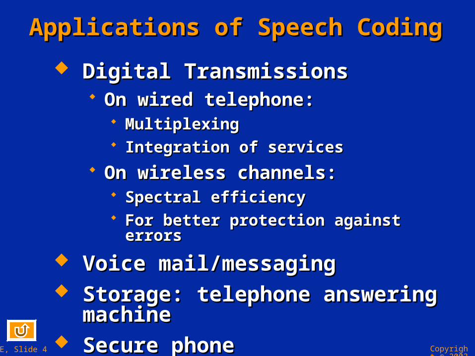
Applications of Speech CodingApplications of Speech Coding

Digital Transmissions Digital Transmissions On wired telephone:On wired telephone:

MultiplexingMultiplexing Integration of servicesIntegration of services

On wireless channels:On wireless channels: Spectral efficiency Spectral efficiency For better protection against errorsFor better protection against errors

Voice mail/messagingVoice mail/messaging Storage: telephone answering machineStorage: telephone answering machine Secure phoneSecure phone


ESIEE, Slide 5

Characteristics of CodersCharacteristics of Coders

Bit Rate D: 50 bps < D < 96 kbpsBit Rate D: 50 bps < D < 96 kbps Coding Delay ~ frame delayCoding Delay ~ frame delay Quality Quality

Objective measurements: SNR, PSQMObjective measurements: SNR, PSQM Subjective measurements: MOS Subjective measurements: MOS

(excellent,good,fair,poor,unacceptable)(excellent,good,fair,poor,unacceptable) Intelligibility:Intelligibility:

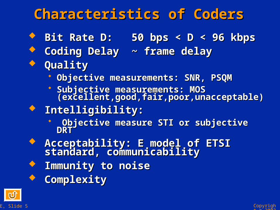
Objective measure STI or subjective DRTObjective measure STI or subjective DRT Acceptability: E model of ETSI standard, Acceptability: E model of ETSI standard,

communicabilitycommunicability Immunity to noiseImmunity to noise ComplexityComplexity


ESIEE, Slide 6

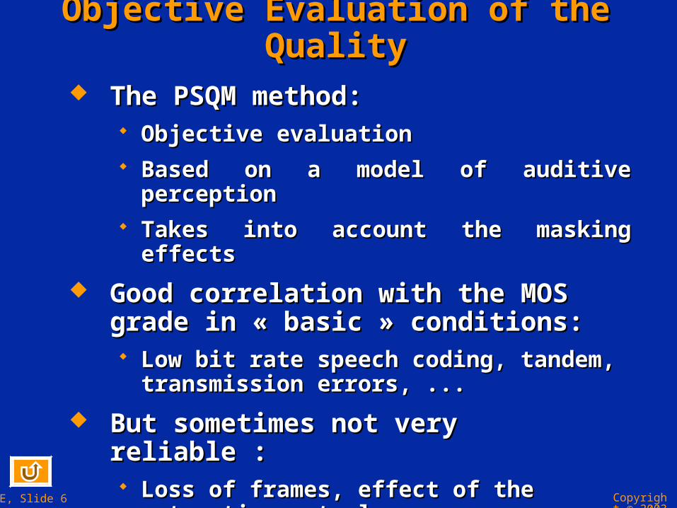
Objective Evaluation of the QualityObjective Evaluation of the Quality

The PSQM method:The PSQM method: Objective evaluationObjective evaluation Based on a model of auditive perceptionBased on a model of auditive perception Takes into account the masking effectsTakes into account the masking effects

Good correlation with the MOS grade in Good correlation with the MOS grade in « basic » conditions:« basic » conditions: Low bit rate speech coding, tandem, transmission Low bit rate speech coding, tandem, transmission

errors, ...errors, ...

But sometimes not very reliable :But sometimes not very reliable : Loss of frames, effect of the automatic controlLoss of frames, effect of the automatic control Still under development (PSQM+)Still under development (PSQM+)


ESIEE, Slide 7

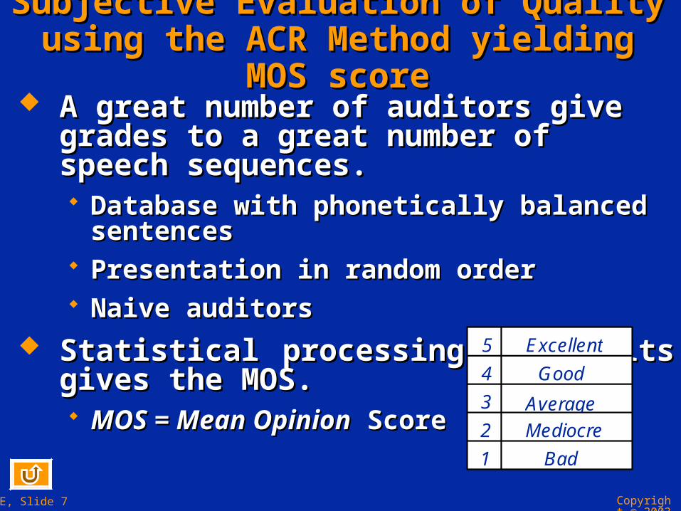
Subjective Evaluation of QualitySubjective Evaluation of Qualityusing the ACR Method yielding MOS scoreusing the ACR Method yielding MOS score A great number of auditors give grades to a A great number of auditors give grades to a

great number of speech sequences. great number of speech sequences. Database with phonetically balanced sentencesDatabase with phonetically balanced sentences Presentation in random orderPresentation in random order Naive auditorsNaive auditors

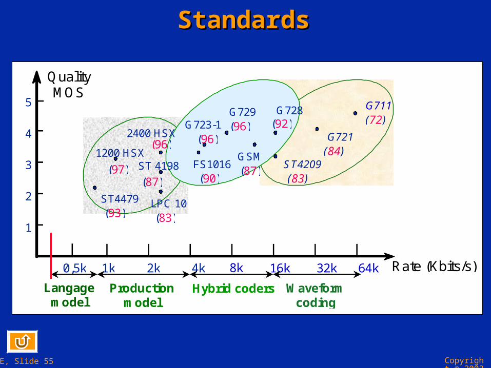
Statistical processing of results gives the MOS.Statistical processing of results gives the MOS. MOS = Mean OpinionMOS = Mean Opinion Score Score

Bad

Mediocre

Average

Good

Excellent

1

2

3

4

5


ESIEE, Slide 8

Speech ProductionSpeech Production

Diaphragm

Lungs Larynx

Vocal chords

Nasal Cavity

Mouth Cavity

Palate

Tongue

Lips

Jaws

Vocal tract

Wind Pipe

Articulators

Wind Tunnel

Oscillator


ESIEE, Slide 9

Speech SignalSpeech Signal


ESIEE, Slide 10

Speech Spectrum for a Voiced SoundSpeech Spectrum for a Voiced Sound


ESIEE, Slide 11

Speech Spectrogram Speech Spectrogram

Non stationaryNon stationary Voiced / unvoicedVoiced / unvoiced


ESIEE, Slide 12

Calculation of SpectrogramsCalculation of Spectrograms

Preac = Preaccentuation, enhances high freqeunciesPreac = Preaccentuation, enhances high freqeuncies

Window = limits the edge effectsWindow = limits the edge effects

Preac Window FFT Log(| |)

Power spectral density

Speech signal

0 2 4 6 8 10 1

2 14 1

6 18 2

0 0

0.1 0.2 0.3 0.4 0.5 0.6 0.7 0.8 0.9 1

Time

Example of window


ESIEE, Slide 13

Example: Time Signal and SpectrogramExample: Time Signal and Spectrogram

1 2 3 4 5 6 7 80

500

1000

1500

2000

2500

3000

3500

0 1 2 3 4 5 6 7 8 9-3

-2

-1

0

1

2

3x 10

4

TimeTime

FrequencyFrequency

TimeTime

SPECTROGRAMSPECTROGRAM

TIME SIGNALTIME SIGNAL


ESIEE, Slide 14

Equivalent Electrical ModelEquivalent Electrical Model

NV

V

Stochastic excitation

Periodical excitation

Speech

Spectrum shaping filter

f

Transfer function of the vocal tract

Voicing

Gain


ESIEE, Slide 15

Simplified Speech Production ModelSimplified Speech Production Model

y(t)=h(t)*e(t) - Y(z)= H(z)E(z)y(t)=h(t)*e(t) - Y(z)= H(z)E(z)

V z e z e zc jb T

k

Kc jb Tk k k k( ) / ( )( )( ) ( )

1 1 11

1

1

L z z( ) 1 1

G z e zcT( ) / ( ) 1 1 1 2

G(z) V(z) L(z)

glottis radiation at the lips

vocal tract yy((tt)) ee((tt))


ESIEE, Slide 16

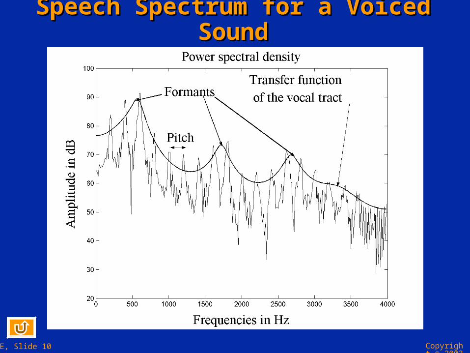
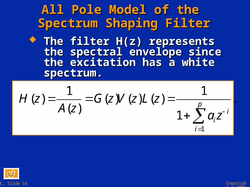
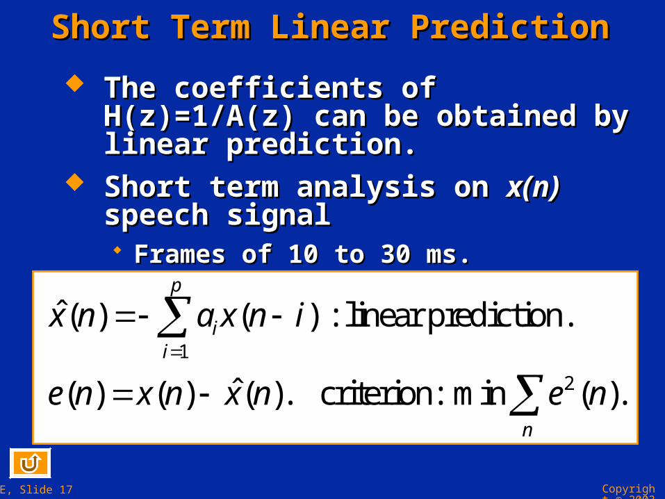
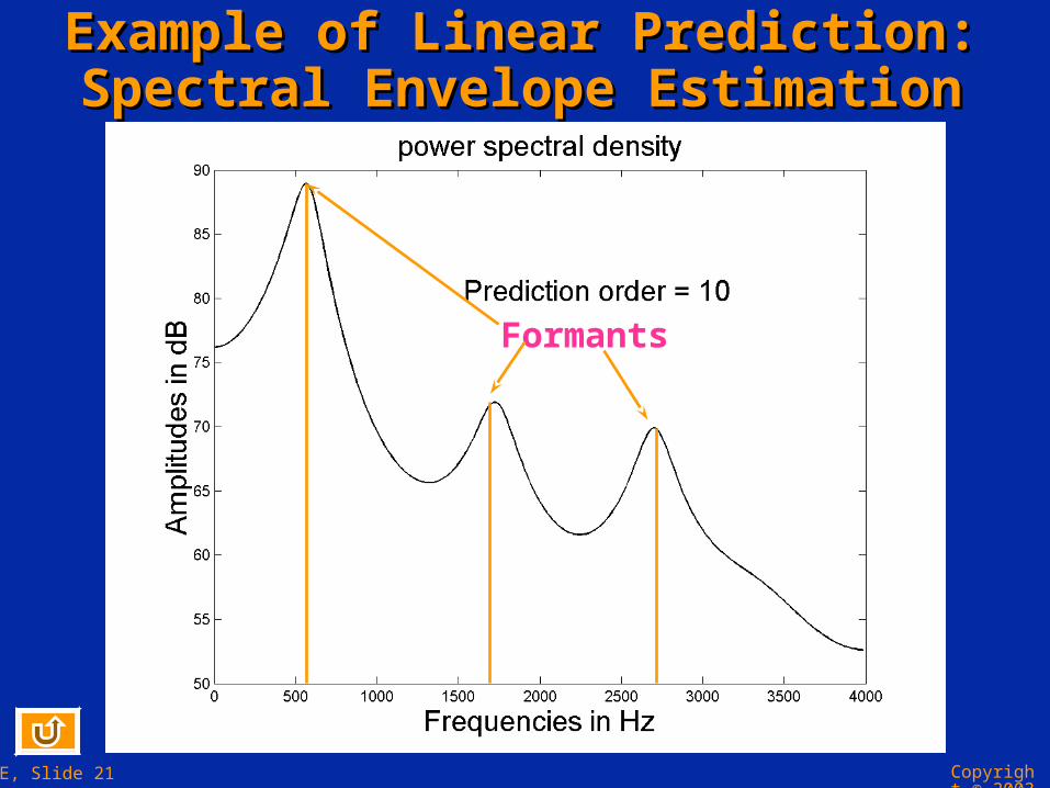
All Pole Model of the All Pole Model of the Spectrum Shaping FilterSpectrum Shaping Filter

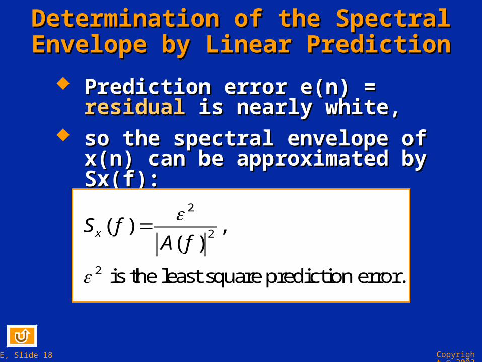
The filter H(z) represents the spectral The filter H(z) represents the spectral envelope since the excitation has a white envelope since the excitation has a white spectrum.spectrum.

1

1 1( ) ( ) ( ) ( ) .

( )1

pi

ii

H z G z V z L zA z

a z


ESIEE, Slide 17

Short Term Linear PredictionShort Term Linear Prediction

The coefficients of H(z)=1/A(z) can be The coefficients of H(z)=1/A(z) can be obtained by linear prediction.obtained by linear prediction.

Short term analysis on Short term analysis on x(n)x(n) speech signal speech signal Frames of 10 to 30 ms.Frames of 10 to 30 ms.

Least square error criterion:Least square error criterion:

1

2

ˆ( ) ( ) : linear prediction.

ˆ( ) ( ) ( ). criterion: min ( ).

p

ii

n

x n a x n i

e n x n x n e n


ESIEE, Slide 18

Determination of the Spectral Envelope by Determination of the Spectral Envelope by Linear PredictionLinear Prediction

Prediction Prediction error e(n) = error e(n) = residualresidual is is nearly white, nearly white,

so the spectral envelope of x(n) can be so the spectral envelope of x(n) can be approximated by Sx(f):approximated by Sx(f):

2

2

2

( ) ,( )

is the least square prediction error.

xS fA f


ESIEE, Slide 19

Calculation of the Prediction CoeffcientsCalculation of the Prediction Coeffcients

The prediction coefficients The prediction coefficients aaii are the are the solution of the «normal equations»:solution of the «normal equations»:

1,1 1, 1 0,1

,1 , 0,

,

.

( ) ( ).

p

p p p p p

i j

r r a r

r r a r

r x n i x n j

The Levinson Durbin algorithm is often The Levinson Durbin algorithm is often used to solve these equationsused to solve these equations


ESIEE, Slide 20

Example of Linear PredictionExample of Linear Prediction

Amplitude of the speech signal

Amplitude of residual signal


ESIEE, Slide 21

Example of Linear Prediction: Spectral Example of Linear Prediction: Spectral Envelope EstimationEnvelope Estimation

Formants


ESIEE, Slide 22

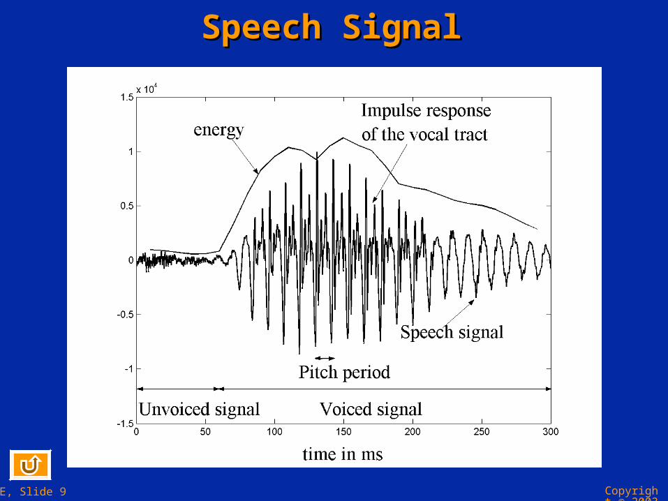
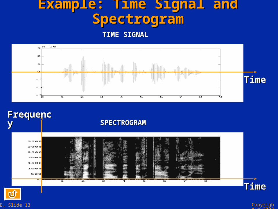
Estimation of the Pitch PeriodEstimation of the Pitch Period

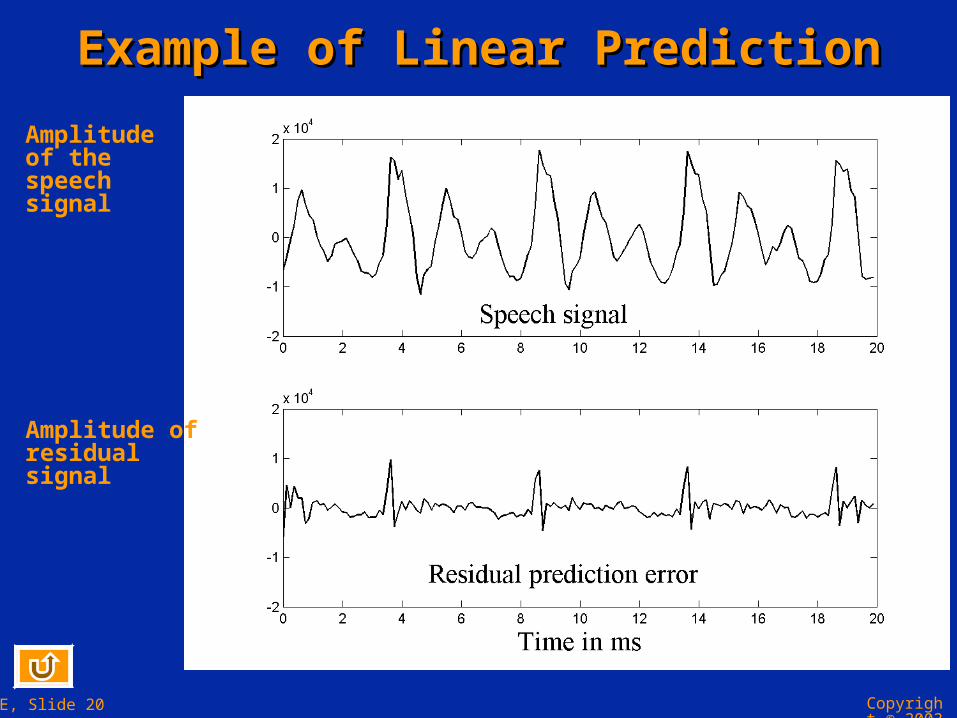
Pitch Period TPitch Period T00 estimated by correlation estimated by correlation of the speech signal or residual.of the speech signal or residual. Other methods exist (e.g. cepstrum)Other methods exist (e.g. cepstrum) FF00 = fundamental frequency = 1/T = fundamental frequency = 1/T00

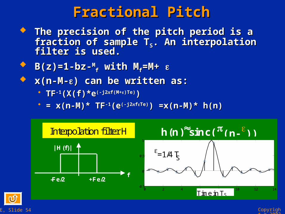
Fractional pitch estimationFractional pitch estimation if the precision if the precision is better than the sampling period.is better than the sampling period.

0

0

50 400

120 160 f 8000 .S

S

Hz F Hz

T kT k i Fs HzT


ESIEE, Slide 23

Long Term Prediction (LTP)Long Term Prediction (LTP)

The idea is to predict one period of The idea is to predict one period of signal from the preceding one:signal from the preceding one:

ˆ( ) ( ).x n b x n M

2 unknowns: b and M.2 unknowns: b and M.M is the pitch period (when voiced).M is the pitch period (when voiced).

Least square error criterion is used.Least square error criterion is used.


ESIEE, Slide 24

Long Term Prediction (LTP)Long Term Prediction (LTP)

2n n M n M

n n

b x x x

2

2

n Mn n Mn n

x x x

For a given value of M, optimal b is:For a given value of M, optimal b is:

The best M value maximizes:The best M value maximizes:

All possible values of M must be tested.All possible values of M must be tested.


ESIEE, Slide 25

Example of Long Term PredictionExample of Long Term Prediction


ESIEE, Slide 26

LPC 10 VocoderLPC 10 Vocoder

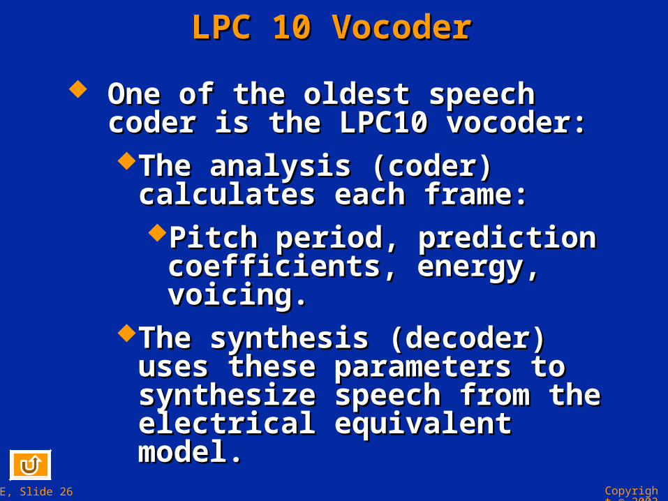
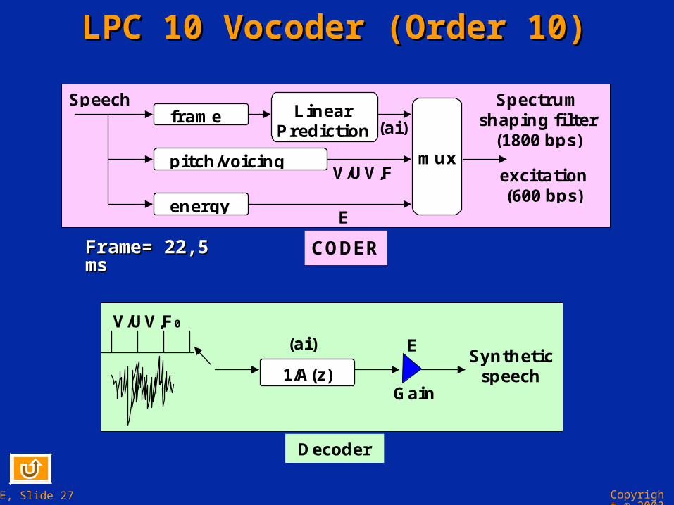
One of the oldest speech coder is the One of the oldest speech coder is the LPC10 vocoder:LPC10 vocoder:The analysis (coder) calculates each The analysis (coder) calculates each

frame:frame:Pitch period, prediction Pitch period, prediction

coefficients, energy, voicing.coefficients, energy, voicing.The synthesis (decoder) uses these The synthesis (decoder) uses these

parameters to synthesize speech from parameters to synthesize speech from the electrical equivalent model.the electrical equivalent model.


ESIEE, Slide 27

LPC 10 Vocoder (Order 10)LPC 10 Vocoder (Order 10)

Speech frame Linear

Prediction

pitch/voicing

energy

mux

(ai)

E

excitation (600 bps)

Spectrum shaping filter

(1800 bps)

V/UV,F0

CODER

V/UV,F0

E (ai)

1/A(z) Gain

Synthetic speech

Decoder

Frame= 22,5 msFrame= 22,5 ms


ESIEE, Slide 28

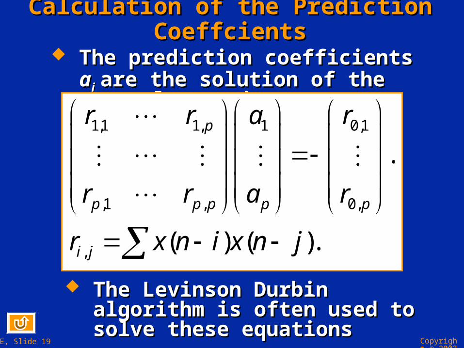
Prediction Spectral ParametersPrediction Spectral Parameters The The aaii coefficients are sensitive to coding and coefficients are sensitive to coding and

interpolation.interpolation. They are replaced by other coefficients:They are replaced by other coefficients:

Reflexion coefficients Reflexion coefficients kkii, log area ratio LARi., log area ratio LARi. Line spectrum frequencies LSFLine spectrum frequencies LSFii..

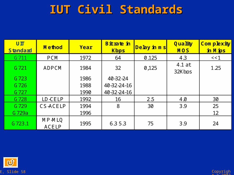
In the LPC10 vocoderIn the LPC10 vocoder The pitch and voicing are coded on 7 bitsThe pitch and voicing are coded on 7 bits The log of energy on 5 bitsThe log of energy on 5 bits The 10 prediction coefficients ai (transformed in The 10 prediction coefficients ai (transformed in

ki and LARi) are coded on 41 bits.ki and LARi) are coded on 41 bits. A total of 53 bits per frame of 22,5ms = 2400bpsA total of 53 bits per frame of 22,5ms = 2400bps


ESIEE, Slide 29

Vector Quantization Vector Quantization (2-dimensional example )(2-dimensional example )

k1

k2

-1

-1

1

1

k1

k2

-1

-1

1

1

* *

*

* *

scalar quantization

. . . . . . . . . . . . . . . . .

.

. . . . . . . . .

.

. . . k1

k2

-1

-1

1

1 . .

. . .

. . .

. .

input vectors (training base)

. . . . . . .

vector quantization the index of the code vector is transmitted

Code vector

Bit rate can be decreased by applying VQ to the coefficients.Bit rate can be decreased by applying VQ to the coefficients.


ESIEE, Slide 30

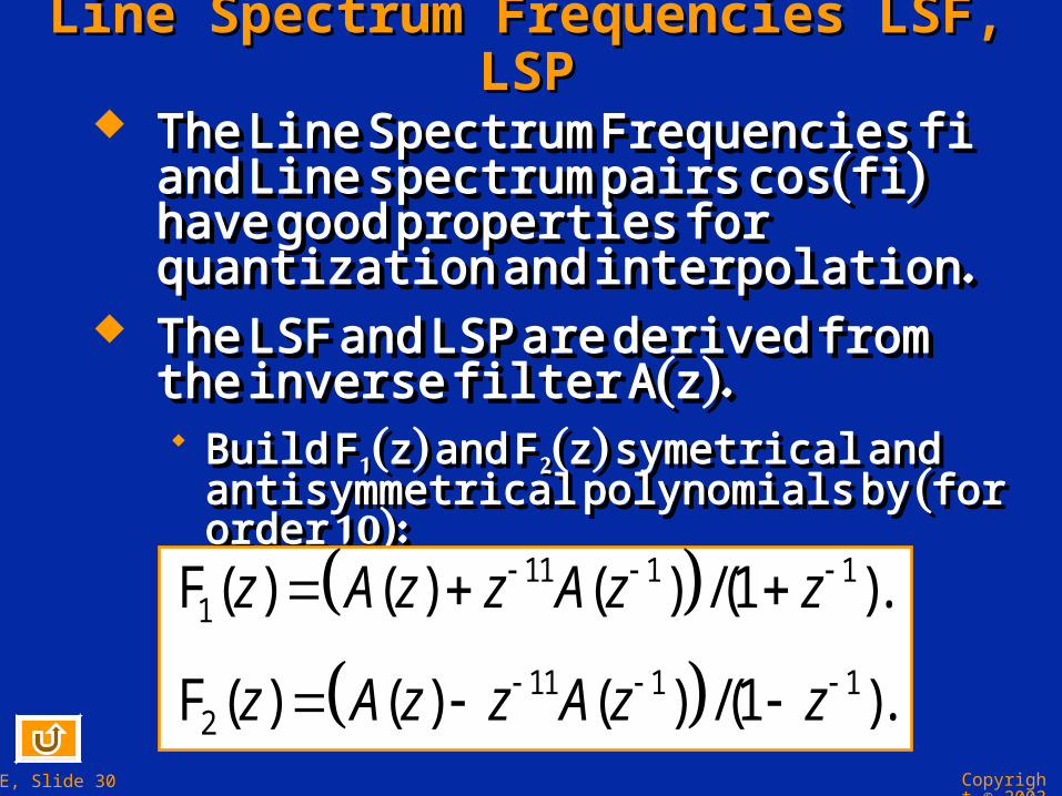
Line Spectrum Frequencies LSF, LSPLine Spectrum Frequencies LSF, LSP

The Line Spectrum Frequencies fi and The Line Spectrum Frequencies fi and Line spectrum pairs cos(fi) have good Line spectrum pairs cos(fi) have good properties for quantization and properties for quantization and interpolation.interpolation.

The LSF and LSP are derived from the The LSF and LSP are derived from the inverse filter A(z).inverse filter A(z). Build FBuild F11(z) and F(z) and F22(z) symetrical and (z) symetrical and

antisymmetrical polynomials by (for order antisymmetrical polynomials by (for order 10):10):

11 1 11

11 1 12

F ( ) ( ) ( ) /(1 ).

F ( ) ( ) ( ) /(1 ).

z A z z A z z

z A z z A z z


ESIEE, Slide 31

LSF and LSPLSF and LSP

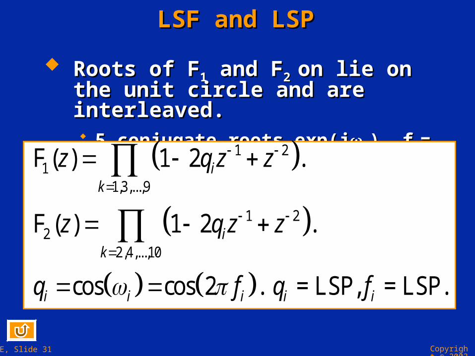
Roots of FRoots of F11 and F and F2 2 on lie on the unit on lie on the unit circle and are interleaved.circle and are interleaved. 5 conjugate roots exp(j5 conjugate roots exp(jii), f), fii= = ii/(2/(2).).

1 21

1,3,...,9

1 22

2,4,...,10

F ( ) 1 2 .

F ( ) 1 2 .

cos cos 2 . = LSP, = LSP.

ik

ik

i i i i i

z q z z

z q z z

q f q f


ESIEE, Slide 32

Coders using Short Term and Long Term Coders using Short Term and Long Term Prediction Prediction RELP RELP MPE LP MPE LPCELPCELP

x(n) e(n) r(n)

Calculation of ri,j and ai

Calculation of b and M

Coding of r(n) u(n) B(z) A(z)

Speech signal

residual signal

Analysis

Quantization of coefficients b, M, ai

Quantized coefficients

Quantized residual

u(n) 1/A(z) 1/B(z)

Synthetic speech signal

Synthesis

Quantized coefficients

Quantized residual


ESIEE, Slide 33

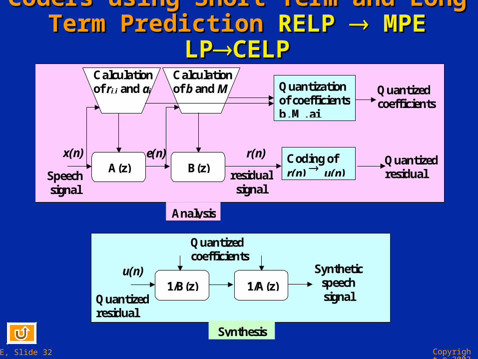
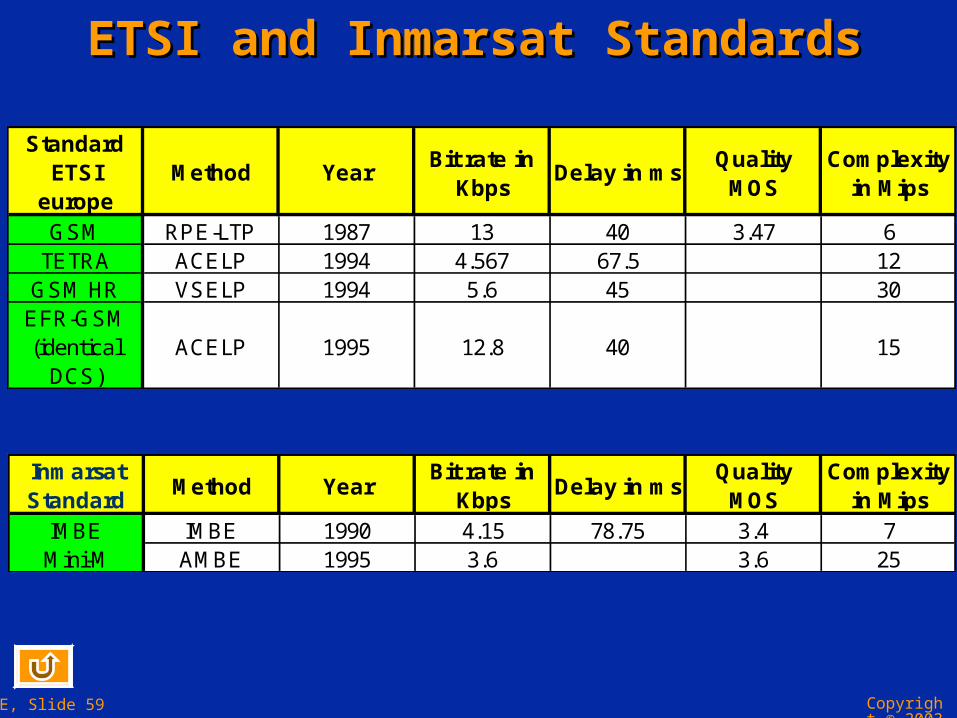
RPE-LTP GSM Full Rate CodersRPE-LTP GSM Full Rate Coders

GSM Full Rate Coder is called:GSM Full Rate Coder is called: RPE LTP= Regular Pulse Excited, Long RPE LTP= Regular Pulse Excited, Long

Term Prediction coderTerm Prediction coder The signal u = the best down-sampled The signal u = the best down-sampled

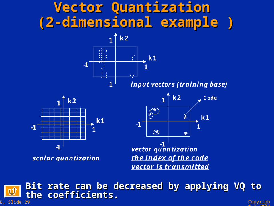
version (version ( 4) of the residual signal r. 4) of the residual signal r. In CELP coders, vector quantization is In CELP coders, vector quantization is

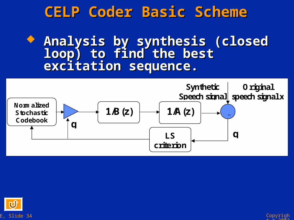
applied on the signal.applied on the signal. CELP = Code Excited Linear Prediction CELP = Code Excited Linear Prediction

codercoder Each frame of residual signal is compared Each frame of residual signal is compared

to sequences of signal stored in a codebook. to sequences of signal stored in a codebook. The codebook sequences are white and the The codebook sequences are white and the codebook is called stochastic codebook.codebook is called stochastic codebook.


ESIEE, Slide 34

CELP Coder Basic SchemeCELP Coder Basic Scheme

Analysis by synthesis (closed loop) to Analysis by synthesis (closed loop) to find the best excitation sequence.find the best excitation sequence.

Normalized Stochastic Codebook

1/A(z) 1/B(z) g

-

LS criterion

q

Original speech signal x

Synthetic Speech signal


ESIEE, Slide 35

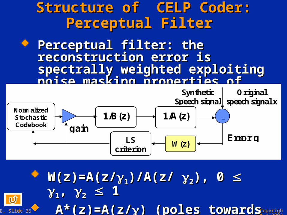
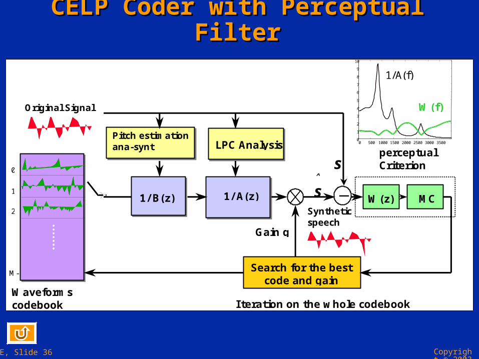
Structure of CELP Coder: Perceptual Filter Structure of CELP Coder: Perceptual Filter

Perceptual filter: the reconstruction error Perceptual filter: the reconstruction error is spectrally weighted exploiting noise is spectrally weighted exploiting noise masking properties of formants.masking properties of formants.

W(z)=A(z/W(z)=A(z/11)/A(z/ )/A(z/ 22), 0 ), 0 11, , 22 1 1 A*(z)=A(z/A*(z)=A(z/) (poles towards zero)) (poles towards zero)

NormalizedStochasticCodebook

1/A(z)1/B(z)gain

-

LScriterion

Error q

Originalspeech signal x

SyntheticSpeech signal

W(z)


ESIEE, Slide 36

CELP Coder with Perceptual FilterCELP Coder with Perceptual Filter

Original Signal

perceptual Criterion

1/ A(z)

LPC Analysis

Synthetic speech

Iteration on the whole codebook

Gain g

Waveforms codebook

0 1 2

M-1

1/ B(z)

Pitch estimation ana-synt

Search for the best code and gain

W(z) MC

s

s

0 500 1000 1500 2000 2500 3000 3500 0 1 2 3 4 5 6 7 8 9

10

W(f)

1/A(f)


ESIEE, Slide 37

Basic CELP Structure: Perceptual Filter Basic CELP Structure: Perceptual Filter Inserted in the 2 BranchesInserted in the 2 Branches

Least Square

g

cj

r

Speech frame

H(z) including

g W(z)

W(z)

e

+ -

s Weighted speech frame

Codebook

1/B(z) e

p

s

H(z)=W(z)/A(z)H(z)=W(z)/A(z)


ESIEE, Slide 38

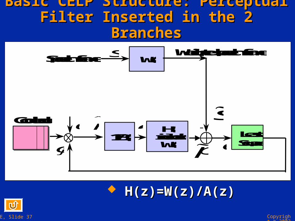
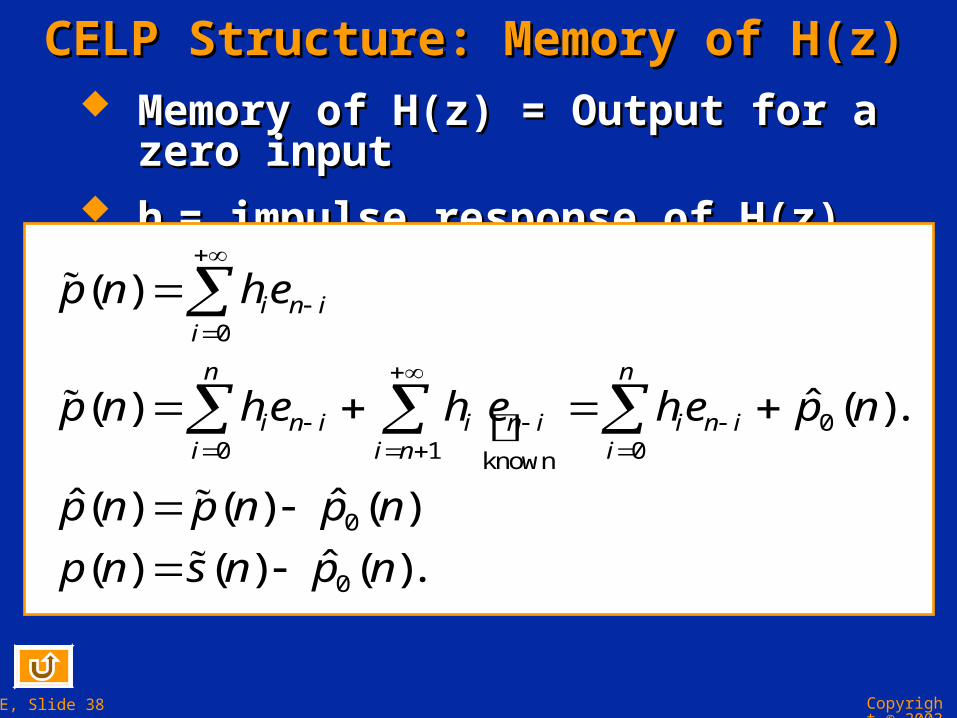
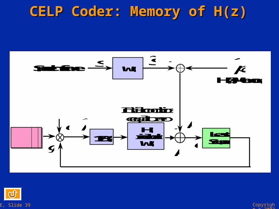
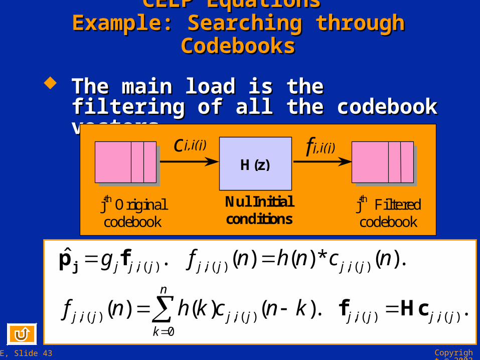
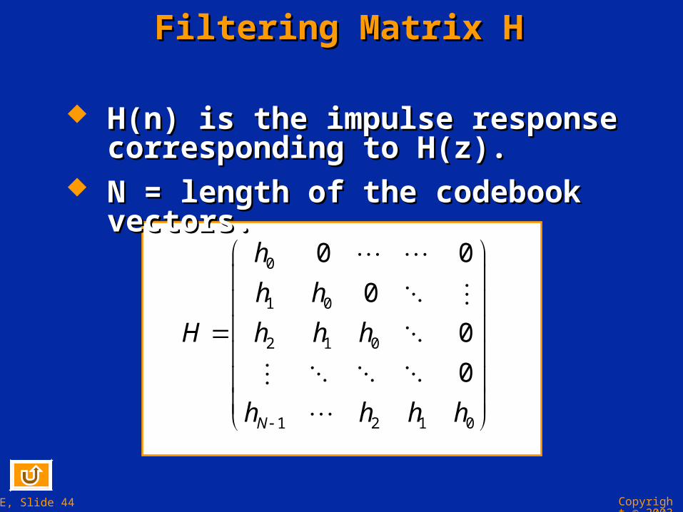
CELP Structure: Memory of H(z)CELP Structure: Memory of H(z) Memory of H(z) = Output for a zero inputMemory of H(z) = Output for a zero input hhii= impulse response of H(z)= impulse response of H(z)

0

00 1 0known

0

0

( )

ˆ( ) ( ).

ˆ ˆ( ) ( ) ( )

ˆ( ) ( ) ( ).

i n ii

n n

i n i i n i i n ii i n i

p n h e

p n h e h e h e p n

p n p n p n

p n s n p n


ESIEE, Slide 39

CELP Coder: Memory of H(z)CELP Coder: Memory of H(z)

Least Square

+ -

g

cj

r

Speech frame

p H(z)

includingg W(z)

W(z)

p e

+ -

p0 H(z) Memory

s

1/B(z)

s

Initial conditions equal to zero


ESIEE, Slide 40

CELP: Adaptive CodebookCELP: Adaptive Codebook LTP can be realized by an adaptive codebookLTP can be realized by an adaptive codebook

0 ( ) 2 1

0 0

ˆ ˆ ˆ ˆ( ) .n n

jn in n i i n i n i M n n

i i

p p h e h gc be p p

1

0

2 ( )

0

ˆ .

ˆ .

n

n i n i Mi

nj

n i n ii

p b h e

p g h c


ESIEE, Slide 41

CELP with Stochastic CodebookCELP with Stochastic Codebook

Least Square

+ -

g 1

g 2

c 1,i(0)

c 2,i(1)

Speech frame

p H(z)

W(z)

p e

+ -

p0

H filter memory

s

H(z)

p1

p2

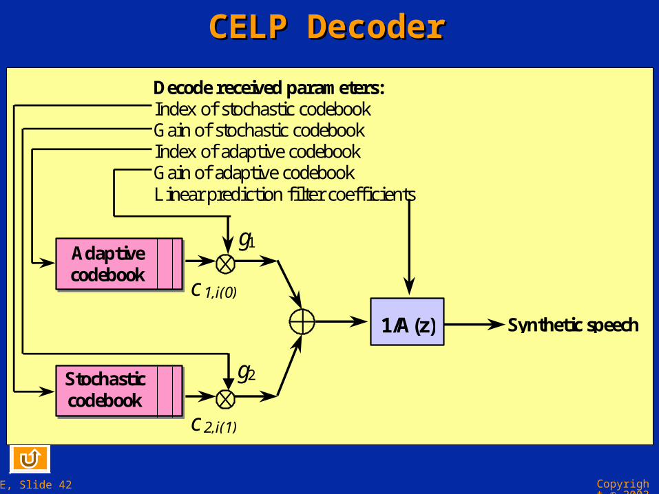
Adaptive codebook

Stochastic codebook

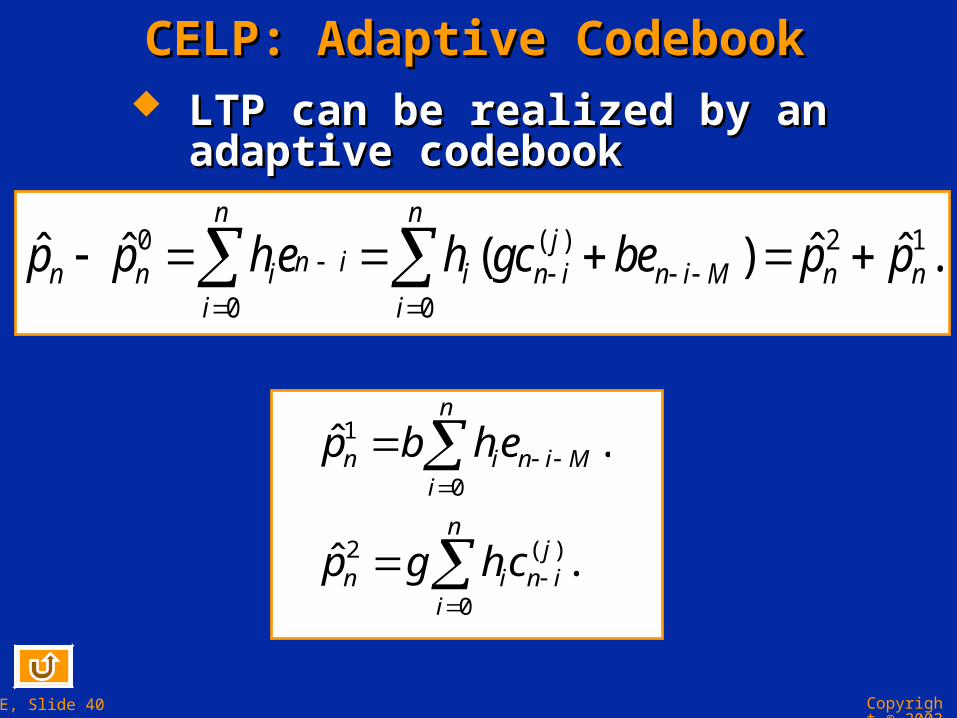
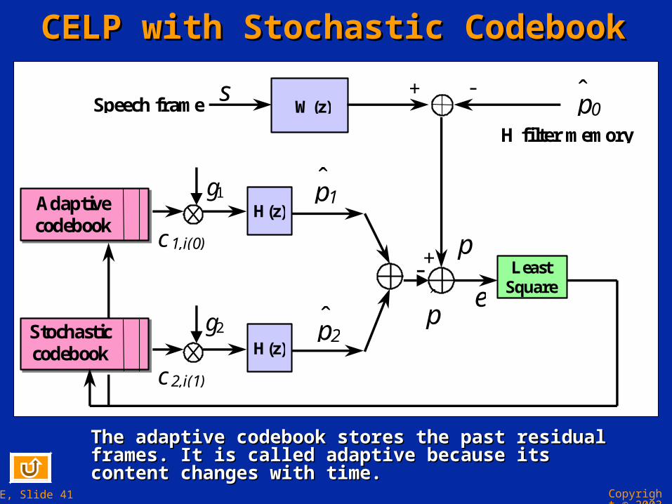
The adaptive codebook stores the past residual frames. It is called The adaptive codebook stores the past residual frames. It is called adaptive because its content changes with timeadaptive because its content changes with time..


ESIEE, Slide 42

CELP DecoderCELP Decoder

g 1

g 2

c 1,i(0)

c 2,i(1)

Synthetic speech 1/A(z)

Adaptive codebook

Stochastic codebook

Decode received parameters: Index of stochastic codebook Gain of stochastic codebook Index of adaptive codebook Gain of adaptive codebook Linear prediction filter coefficients


ESIEE, Slide 43

CELP Equations CELP Equations Example: Searching through CodebooksExample: Searching through Codebooks

The main load is the filtering of all the The main load is the filtering of all the codebook vectors.codebook vectors.

c j,i(j) H(z)

Nul Initial conditions

f j,i(j)

jth Filtered codebook

jth Original codebook

, ( ) , ( ) , ( )

, ( ) , ( ) , ( ) , ( )0

ˆ . ( ) ( )* ( ).

( ) ( ) ( ). .

j j i j j i j j i j

n

j i j j i j j i j j i jk

g f n h n c n

f n h k c n k

jp f

f Hc


ESIEE, Slide 44

Filtering Matrix HFiltering Matrix H

0

1 0

2 1 0

1 2 1 0

0 0

0

0

0

N

h

h h

H h h h

h h h h

H(n) is the impulse response H(n) is the impulse response corresponding to H(z).corresponding to H(z).

N = length of the codebook vectors.N = length of the codebook vectors.


ESIEE, Slide 45

Finding the Best Excitation in the Coder:Finding the Best Excitation in the Coder:Equation of the SolutionEquation of the Solution

J least square criterionJ least square criterion For a set of 2 vectors For a set of 2 vectors ccj,i(j)j,i(j), F is the 2 , F is the 2

column matrix of filtered vectors column matrix of filtered vectors ffj,i(j)j,i(j)

2 2

2 1

ˆ

Optimal gain:

ˆmin max ( )

T T

T T T

J p p p Fg

F F g F p

J p p F F F F p


ESIEE, Slide 46

CELP Optimal SolutionCELP Optimal Solution

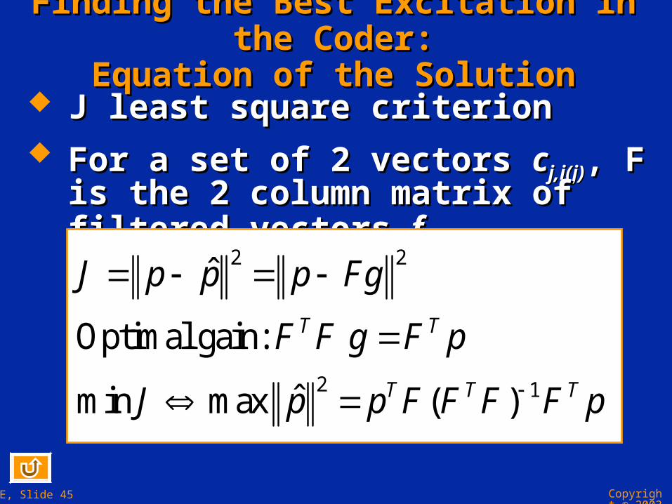
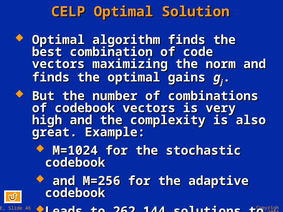
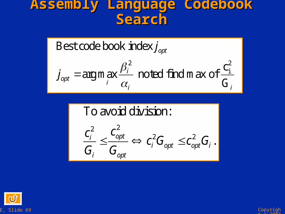
Optimal algorithm finds the best Optimal algorithm finds the best combination of code vectors maximizing combination of code vectors maximizing the norm and finds the optimal gains the norm and finds the optimal gains ggjj..

But the number of combinations of But the number of combinations of codebook vectors is very high and the codebook vectors is very high and the complexity is also great. Example:complexity is also great. Example: M=1024 for the stochastic codebookM=1024 for the stochastic codebook and M=256 for the adaptive codebookand M=256 for the adaptive codebookLeads to 262 144 solutions to test andLeads to 262 144 solutions to test and1280 vectors to filter.1280 vectors to filter.


ESIEE, Slide 47

Iterative Suboptimal Algorithm for 2 Iterative Suboptimal Algorithm for 2 CodebooksCodebooks

First step:First step: Target vector = pTarget vector = p Find the best vector in the adaptive Find the best vector in the adaptive

codebook and its gain.codebook and its gain. Calculate the new target vector p1:Calculate the new target vector p1:

11 ˆn np p p

Second step: Second step: Target vector = p1Target vector = p1Find the best vector in the stochastic Find the best vector in the stochastic

codebook and its gain.codebook and its gain.


ESIEE, Slide 48

Iterative AlgorithmIterative Algorithm

-

H(z)

W(z)

p2 g2

p0

Speech

c(n,j)

j,g1

H(z) p1 g1 e(n-M)

LSS

M,g2

+ g1

g2

p

p1

LSS


ESIEE, Slide 49

Operations of the Iterative AlgorithmOperations of the Iterative Algorithm

At step j, the optimal codebook vector At step j, the optimal codebook vector has index i:has index i:

2 2

,ˆarg min =j j j j j kk

i g p p p f

, ,opt,

, , , ,

.T Tj j k j j k

k T Tj k j k j k j k

g T

p f p Hc

f f c H Hc

22

opt,, ,

arg max with Tj j k k

kT Tkj k j k k k

i g

p Hc

c H Hc


ESIEE, Slide 50


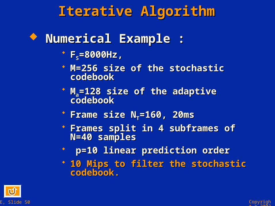
Numerical Example :Numerical Example : FFSS=8000Hz,=8000Hz, M=256 size of the stochastic codebookM=256 size of the stochastic codebook MMaa=128 size of the adaptive codebook=128 size of the adaptive codebook Frame size NFrame size NTT=160, 20ms=160, 20ms Frames split in 4 subframes of N=40 samplesFrames split in 4 subframes of N=40 samples p=10 linear prediction orderp=10 linear prediction order 10 Mips to filter the stochastic codebook.10 Mips to filter the stochastic codebook.


ESIEE, Slide 51


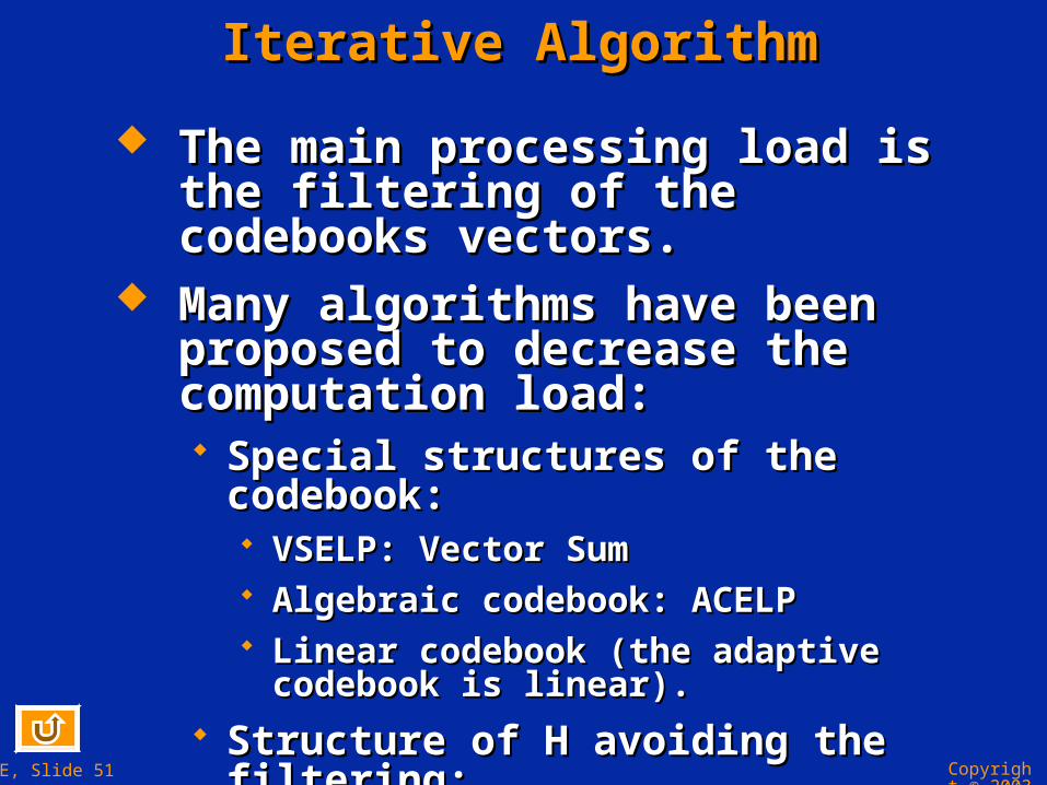
The main processing load is the filtering The main processing load is the filtering of the codebooks vectors.of the codebooks vectors.

Many algorithms have been proposed to Many algorithms have been proposed to decrease the computation load:decrease the computation load: Special structures of the codebook:Special structures of the codebook:

VSELP: Vector SumVSELP: Vector Sum Algebraic codebook: ACELPAlgebraic codebook: ACELP Linear codebook (the adaptive codebook is Linear codebook (the adaptive codebook is

linear).linear).

Structure of H avoidStructure of H avoidiing the filtering:ng the filtering: Diagonalization of HDiagonalization of HTTHH


ESIEE, Slide 52

CELP CodingCELP Coding

Standards from 4.8 kbps to 16 kbpsStandards from 4.8 kbps to 16 kbps Federal standard (DOD) (4.8 kbps)Federal standard (DOD) (4.8 kbps)

frame = 260 samples (30 ms)frame = 260 samples (30 ms) LPC 8 --> (LSP coding 34 bits)LPC 8 --> (LSP coding 34 bits) adaptive codebook (256 vectors (fractional adaptive codebook (256 vectors (fractional

pitch))pitch)) stochastic codebook (512 vectors (-1,0,1))stochastic codebook (512 vectors (-1,0,1))


ESIEE, Slide 53

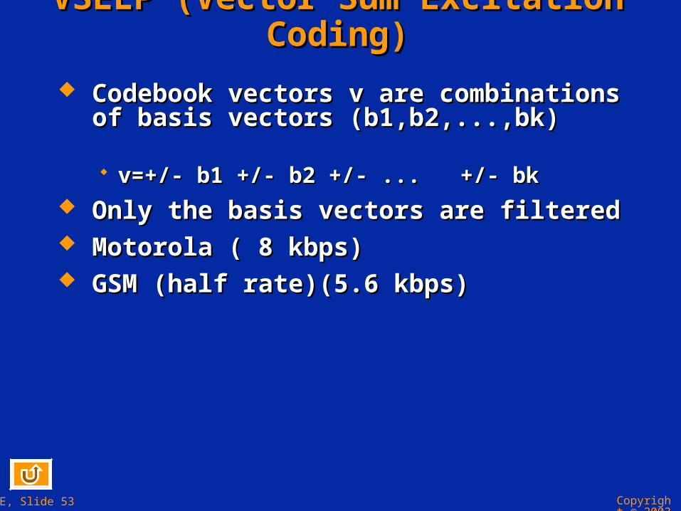
VSELP (Vector Sum Excitation Coding)VSELP (Vector Sum Excitation Coding)

Codebook vectors v are combinations of Codebook vectors v are combinations of basis vectors (b1,b2,...,bk) basis vectors (b1,b2,...,bk) v=+/- b1 +/- b2 +/- ... +/- bkv=+/- b1 +/- b2 +/- ... +/- bk

Only the basis vectors are filteredOnly the basis vectors are filtered Motorola ( 8 kbps)Motorola ( 8 kbps) GSM (half rate)(5.6 kbps)GSM (half rate)(5.6 kbps)


ESIEE, Slide 54

Fractional PitchFractional Pitch The precision of the pitch period is a fraction of The precision of the pitch period is a fraction of

sample Tsample TSS. An interpolation filter is used.. An interpolation filter is used. B(z)=1-bz-B(z)=1-bz-MM

ff with M with Mff=M+ =M+ x(n-M-x(n-M-) can be written as:) can be written as:

TFTF-1-1(X(f)*e(X(f)*e(-j2(-j2f(M+f(M+)Te))Te))) = x(n-M)* TF= x(n-M)* TF-1-1(e(e(-j2(-j2ffTe)Te)) =x(n-M)* h(n)) =x(n-M)* h(n)

h(n)sinc((n-))

+Fe/2 -Fe/2 f

| H(f)|

Interpolation filter H H(f)

0 2 4 6 8 10 12 14 -0.5

0

0.5

1

=1/4 T S

Time in TS


ESIEE, Slide 55

StandardsStandards

Rate (Kbits/s) 1k 2k 4k 16k 32k 64k

Quality MOS

Production model

Hybrid coders Waveform coding

1

2

3

4

5 G711 (72)

G721 (84)

ST4209 (83)

G728 (92)

(90)

G729 (96)

ST4479 (93)

ST 4198

(87)

2400 HSX (96)

LPC 10 (83)

GSM (87)

1200 HSX

(97)

G723-1 (96)

0,5k

Langage model

8k

FS1016


ESIEE, Slide 56

StandardsStandards Wired Telephony UIT-T Wired Telephony UIT-T

G 711 (1972)G 711 (1972) : PCM: PCM 64 kbps64 kbps G 721 (1984)G 721 (1984) : ADPCM: ADPCM 32 kbps32 kbps G 728 (1991)G 728 (1991) : LD_CELP: LD_CELP 16 kbps 16 kbps G 729G 729 : CS-ACELP: CS-ACELP 8 kbps 8 kbps

Mobile communications (ETSI - CTIA)Mobile communications (ETSI - CTIA) GSM (FR ) GSM (FR ) :RPE_LTP :RPE_LTP 13 kbps13 kbps GSM (HR) GSM (HR) :VSELP:VSELP 5.6 kbps5.6 kbps GSM (EFR) GSM (EFR) : ACELP : ACELP 12.2 kbps12.2 kbps UMTS (AMR) : ACELPUMTS (AMR) : ACELP 12.2 to 4.75 Kbps12.2 to 4.75 Kbps

Military applications (NATO)Military applications (NATO) FS 1015 (1976)FS 1015 (1976) : LPC10: LPC10 2.4 kbps2.4 kbps FS 1016 (1991)FS 1016 (1991) : CELP: CELP 4.8 kbps4.8 kbps


ESIEE, Slide 57

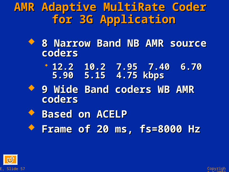
AMR Adaptive MultiRate Coder AMR Adaptive MultiRate Coder for 3G Applicationfor 3G Application

8 Narrow Band NB AMR source coders8 Narrow Band NB AMR source coders 12.2 10.2 7.95 7.40 6.70 5.90 5.15 4.75 kbps12.2 10.2 7.95 7.40 6.70 5.90 5.15 4.75 kbps

9 Wide Band coders WB AMR coders9 Wide Band coders WB AMR coders Based on ACELPBased on ACELP Frame of 20 ms, fs=8000 HzFrame of 20 ms, fs=8000 Hz


ESIEE, Slide 58

IUT Civil StandardsIUT Civil Standards

UIT Standard

Method YearBit rate in

KbpsDelay in ms

Quality MOS

Complexity in Mips

G711 PCM 1972 64 0.125 4.3 <<1

G721 ADPCM 1984 32 0,1254.1 at

32Kbps1.25

G723 1986 40-32-24G726 1988 40-32-24-16G727 1990 40-32-24-16G728 LD-CELP 1992 16 2.5 4.0 30G729 CS-ACELP 1994 8 30 3.9 25

G729a 1996 12

G723.1MP-MLQ ACELP

1995 6.3 5.3 75 3.9 24


ESIEE, Slide 59

ETSI and Inmarsat StandardsETSI and Inmarsat Standards

Inmarsat Standard

Method YearBit rate in

KbpsDelay in ms

Quality MOS

Complexity in Mips

IMBE IMBE 1990 4.15 78.75 3.4 7Mini-M AMBE 1995 3.6 3.6 25

Standard ETSI

europeMethod Year

Bit rate in Kbps

Delay in msQuality

MOSComplexity

in Mips

GSM RPE-LTP 1987 13 40 3.47 6TETRA ACELP 1994 4.567 67.5 12

GSM HR VSELP 1994 5.6 45 30EFR-GSM (identical

DCS)ACELP 1995 12.8 40 15


ESIEE, Slide 60

TIA and RCR StandardsTIA and RCR Standards

TIA standard

USAMethod Year

Bit rate in Kbps

Delay in msQuality

MOSComplexity

in Mips

IS54 VSELP 1989 7.95 45 3.5 20IS96 QCELP 1993 8.5-4.2-0.8 45 4 20

IS136 ACELP 1995 7.4 45IS127 EVRC RCELP 1995 8.5-4-0.8 >45 20PCS 1900 ACELP 1995 40 15

TIA standard

USAMethod Year

Bit rate in Kbps

Delay in msQuality

MOSComplexity

in Mips

RCR STD-27B

VSELP 1990 6.7 45 20

JDC HR PSI-CELP 1993 3.45 90 50


ESIEE, Slide 61

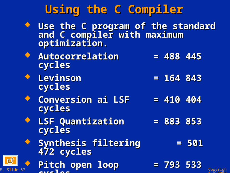
Implementation of CELP Coders on C54xImplementation of CELP Coders on C54x

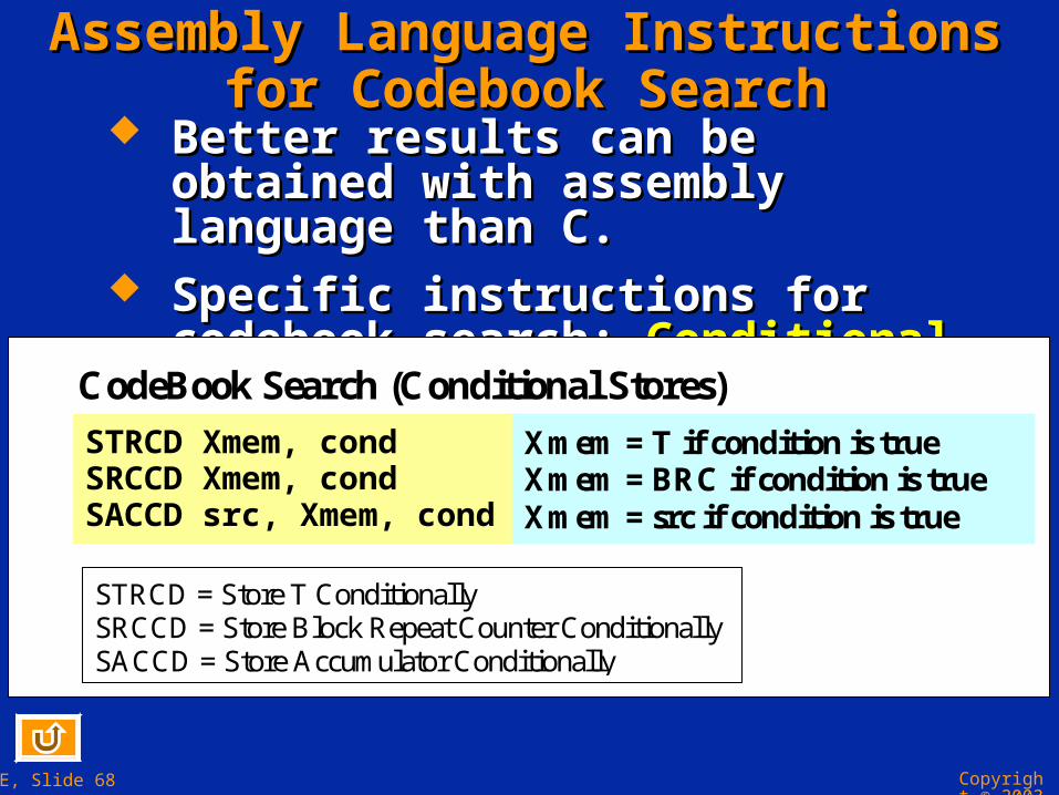
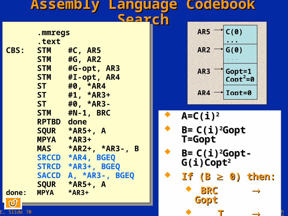
Example of the G729 Annex A.Example of the G729 Annex A. Specific instruction for codebook search Specific instruction for codebook search Some functions of DSPLIBSome functions of DSPLIB


ESIEE, Slide 62

Profiling Example for G729 Annex AProfiling Example for G729 Annex A using C Compiler using C Compiler

G729 is a CS-ACELP Coder (ITU 1995)G729 is a CS-ACELP Coder (ITU 1995) 8Kbps with quality of ADPCM at 8Kbps with quality of ADPCM at

32Kbps G726. 32Kbps G726. DSVD: G729 Annex A voice over DSVD: G729 Annex A voice over

internet, voice e-mailinternet, voice e-mail Digital Simultaneous Voice & DataDigital Simultaneous Voice & Data


ESIEE, Slide 63

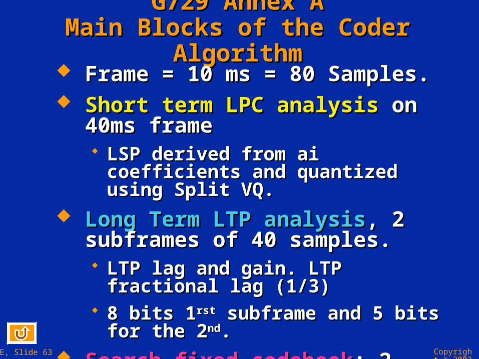
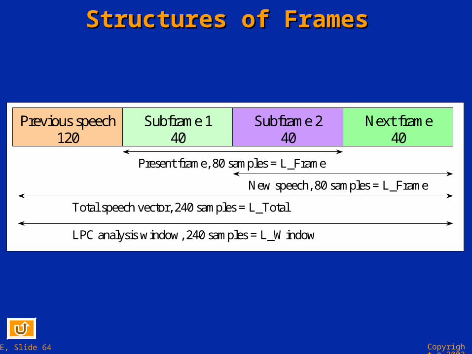
G729 Annex AG729 Annex AMain Blocks of the Coder AlgorithmMain Blocks of the Coder Algorithm Frame = 10 ms = 80 Samples.Frame = 10 ms = 80 Samples. Short term LPC analysisShort term LPC analysis on 40ms frame on 40ms frame

LSP derived from ai coefficients and LSP derived from ai coefficients and quantized using Split VQ.quantized using Split VQ.

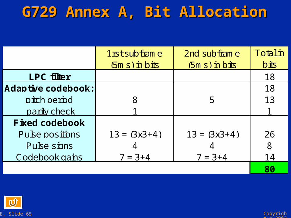
Long Term LTP analysisLong Term LTP analysis, 2 subframes , 2 subframes of 40 samples. of 40 samples. LTP lag and gain. LTP fractional lag (1/3)LTP lag and gain. LTP fractional lag (1/3) 8 bits 18 bits 1rstrst subframe and 5 bits for the 2 subframe and 5 bits for the 2ndnd..

Search fixed codebookSearch fixed codebook: 2 subframes of : 2 subframes of 40 samples. Index and gains40 samples. Index and gains Code length = 40 with 4 non-zero pulses Code length = 40 with 4 non-zero pulses 1.1.


ESIEE, Slide 64

Structures of Frames Structures of Frames

Previous speech 120

Subframe 1 40

Subframe 2 40

Next frame 40

Present frame, 80 samples = L_Frame

New speech, 80 samples = L_Frame

Total speech vector, 240 samples = L_Total

LPC analysis window, 240 samples = L_Window


ESIEE, Slide 65

G729 Annex A, Bit AllocationG729 Annex A, Bit Allocation

Total in bits1818131

2681480

1rst subframe (5ms) in bits

2nd subframe (5ms) in bits

LPC filter

pitch period parity check

Fixed codebookPulse positions

Pulse signsCodebook gains

81

7 = 3+44

Adaptive codebook:

7 = 3+4

13 = (3x3+4)

5

13 = (3x3+4)4


ESIEE, Slide 66

G729 Annex AG729 Annex AMain Blocks of the Decoder AlgorithmMain Blocks of the Decoder Algorithm

The serial received bits are converted into The serial received bits are converted into parameters:parameters: LSP vector, 2 fractional pitch lags and gains, 2 LSP vector, 2 fractional pitch lags and gains, 2

fixed codebook index and gains.fixed codebook index and gains.

LSP are converted to LP filter coefficients LSP are converted to LP filter coefficients ai and interpolated at each subframe.ai and interpolated at each subframe.

At each subframe:At each subframe: The excitation is constructed and scaled.The excitation is constructed and scaled. The speech is synthesized by filtering the The speech is synthesized by filtering the

excitation by the LP synthesis filter.excitation by the LP synthesis filter.

Postprocessing by an adaptive postfilter.Postprocessing by an adaptive postfilter.


ESIEE, Slide 67

Using the C CompilerUsing the C Compiler Use the C program of the standard and C Use the C program of the standard and C

compiler with maximum optimization.compiler with maximum optimization. Autocorrelation Autocorrelation = 488 445 cycles= 488 445 cycles Levinson Levinson = 164 843 cycles= 164 843 cycles Conversion ai LSFConversion ai LSF = 410 404 cycles= 410 404 cycles LSF Quantization LSF Quantization = 883 853 cycles= 883 853 cycles Synthesis filteringSynthesis filtering = 501 472 cycles= 501 472 cycles Pitch open loopPitch open loop = 793 533 cycles= 793 533 cycles Fractional PitchFractional Pitch = 2 x 618 354 cycles= 2 x 618 354 cycles Search Algebraic codeSearch Algebraic code = 2x 617 582 cycles= 2x 617 582 cycles Gains quantizationGains quantization = 2x 108 480 = 2x 108 480

cyclescycles


ESIEE, Slide 68

Assembly Language Instructions for Assembly Language Instructions for Codebook SearchCodebook Search

Better results can be obtained with Better results can be obtained with assembly language than C.assembly language than C.

Specific instructions for codebook Specific instructions for codebook search: search: Conditional storesConditional stores..

CodeBook Search (Conditional Stores) STRCD Xmem, cond SRCCD Xmem, cond SACCD src, Xmem, cond

Xmem = T if condition is true Xmem = BRC if condition is true Xmem = src if condition is true

STRCD = Store T Conditionally SRCCD = Store Block Repeat Counter Conditionally SACCD = Store Accumulator Conditionally


ESIEE, Slide 69

Assembly Language Codebook SearchAssembly Language Codebook Search

2 2i

Best code book index

carg max noted find max of

G

opt

iopt

ii i

j

j

222 2

To avoid division:

.optii opt opt i

i opt

ccc G c G

G G


ESIEE, Slide 70

Assembly Language Codebook SearchAssembly Language Codebook Search .mmregs .text CBS: STM #C, AR5 STM #G, AR2 STM #G-opt, AR3 STM #I-opt, AR4 ST #0, *AR4 ST #1, *AR3+ ST #0, *AR3- STM #N-1, BRC RPTBD done SQUR *AR5+, A MPYA *AR3+ MAS *AR2+, *AR3-, B SRCCD *AR4, BGEQ STRCD *AR3+, BGEQ SACCD A, *AR3-, BGEQ

SQUR *AR5+, A done: MPYA *AR3+

AR5 C(0) ...

AR3 Gopt=1 Copt2=0

AR4 Iopt=0

AR2 G(0) ...

A=C(i)A=C(i)22

B=B= C(i)C(i)22Gopt T=GoptGopt T=Gopt B=B= C(i)C(i)22Gopt-G(i)CoptGopt-G(i)Copt22

If (B If (B 0) then: 0) then: BRC BRC

GoptGopt T T Iopt Iopt A A

CoptCopt22

Date post:	25-Dec-2015
Category:	Documents
Upload:	irene-gaines
View:	215 times
Download:	1 times

DSP C5000 Chapter 23 Mobile Communication Speech Coders Copyright © 2003 Texas Instruments. All...

Documents