Lab P5: Synthesis of Sinusoidal Signals—Music Synthesis
Pre-Lab andWarm-Up: You should read at least the Pre-Lab and Warm-up sections of this lab assignmentand go over all exercises in the Pre-Lab section before going to your assigned lab session.
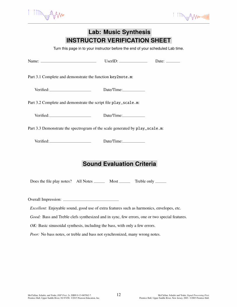
Verification: The Warm-up section of each lab must be completed during your assigned Lab time andthe steps marked Instructor Verification must also be signed off during the lab time. One of the laboratoryinstructors must verify the appropriate steps by signing on the Instructor Verification line. When youhave completed a step that requires verification, simply demonstrate the step to the instructor. Turn in thecompleted verification sheet to your instructor when you leave the lab.
Lab Report: Write a lab report on Section 4 with graphs and explanations. Please label the axes of yourplots and include a title for every plot. In order to keep track of plots, include each plot inlined within yourreport. If you are unsure about what is expected, ask the instructor who will grade your report.
1 Introduction
This lab includes a project on music synthesis with sinusoids. The piece, Fugue #2 for the Well-TemperedClavier by Bach1 has been selected for doing the synthesis program. The project requires an extensiveprogramming effort and should be documented in detail with an formal lab report. A good report shouldinclude the following items: a cover sheet, commented Matlab code, explanations of your approach,conclusions and any additional tweaks that you implemented for the synthesis. Since the project must beevaluated by listening to the quality of the synthesized song, the criteria for judging a good song are givenat the end of this lab description. In addition, it may be convenient to place the final song on a web site sothat it can be accessed remotely by a lab instructor who can then evaluate its quality. If you would like to tryother songs, the DSP First companion website includes information about alternative tunes: Minuet in G,Für Elise, Beethoven’s Fifth, Jesu, Joy of Man’s Desiring and Twinkle, Twinkle, Little Star.
The music synthesis will be done with sinusoidal waveforms of the form
x.t/ DX
k
Ak cos.!kt C 'k/ (1)
so it will be necessary to establish the connection between musical notes, their frequencies, and sinusoids.A secondary objective of the lab is the challenge of trying to add other features to the synthesis in order toimprove the subjective quality for listening. Students who take this challenge will be motivated to learn moreabout the spectral representation of signals—a topic that underlies this entire course.
2 Pre-Lab
In this lab, the periodic waveforms and music signals will be created with the intention of playing them outthrough a loudspeaker. Therefore, it is necessary to take into account the fact that a conversion is neededfrom the digital samples, which are numbers stored in the computer memory to the actual voltage waveformthat will be amplified for the speakers.
1See http://www.jsbach.org/ or https://en.wikipedia.org/wiki/Johann_Sebastian_Bach.
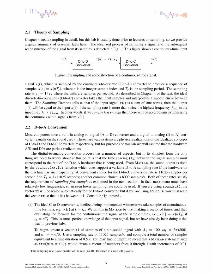
Chapter 4 treats sampling in detail, but this lab is usually done prior to lectures on sampling, so we providea quick summary of essential facts here. The idealized process of sampling a signal and the subsequentreconstruction of the signal from its samples is depicted in Fig. 1. This figure shows a continuous-time input
- - -C-to-DConverter
D-to-CConverter
x.t/ xŒn� D x.nTs/ y.t/
Figure 1: Sampling and reconstruction of a continuous-time signal.
signal x.t/, which is sampled by the continuous-to-discrete (C-to-D) converter to produce a sequence ofsamples xŒn� D x.nTs/, where n is the integer sample index and Ts is the sampling period. The samplingrate is fs D 1=Ts where the units are samples per second. As described in Chapter 4 of the text, the idealdiscrete-to-continuous (D-to-C) converter takes the input samples and interpolates a smooth curve betweenthem. The Sampling Theorem tells us that if the input signal x.t/ is a sum of sine waves, then the outputy.t/ will be equal to the input x.t/ if the sampling rate is more than twice the highest frequency fmax in theinput, i.e., fs > 2fmax. In other words, if we sample fast enough then there will be no problems synthesizingthe continuous audio signals from xŒn�.
2.2 D-to-A Conversion
Most computers have a built-in analog-to-digital (A-to-D) converter and a digital-to-analog (D-to-A) con-verter (usually on the sound card). These hardware systems are physical realizations of the idealized conceptsof C-to-D and D-to-C converters respectively, but for purposes of this lab we will assume that the hardwareA/D and D/A are perfect realizations.
The digital-to-analog conversion process has a number of aspects, but in its simplest form the onlything we need to worry about at this point is that the time spacing .Ts/ between the signal samples mustcorrespond to the rate of the D-to-A hardware that is being used. From Matlab, the sound output is doneby the soundsc(xx,fs) function which does support a variable D-to-A sampling rate if the hardware onthe machine has such capability. A convenient choice for the D-to-A conversion rate is 11025 samples persecond,2 so Ts D 1=11025 seconds; another common choice is 8000 samples/s. Both of these rates satisfythe requirement of sampling fast enough as explained in the next section. In fact, most piano notes haverelatively low frequencies, so an even lower sampling rate could be used. If you are using soundsc(), thevector xxwill be scaled automatically for the D-to-A converter, but if you are using sound.m, you must scalethe vector xx so that it lies between˙1. Consult help sound.
(a) The ideal C-to-D converter is, in effect, being implemented whenever we take samples of a continuous-time formula, e.g., x.t/ at t D tn. We do this in Matlab by first making a vector of times, and thenevaluating the formula for the continuous-time signal at the sample times, i.e., xŒn� D x.nTs/ iftn D nTs . This assumes perfect knowledge of the input signal, but we have already been doing it thisway in previous labs.To begin, create a vector x1 of samples of a sinusoidal signal with A1 D 100, !1 D 2�.800/,and '1 D ��=3. Use a sampling rate of 11025 samples/s, and compute a total number of samplesequivalent to a time duration of 0.5 s. You may find it helpful to recall that a Matlab statement suchas tt=(0:0.01:3); would create a vector of numbers from 0 through 3 with increments of 0.01.
2This sampling rate is one quarter of the rate (44,100 Hz) used in audio CD players.
Therefore, it is only necessary to determine the time increment needed to obtain 11025 samples in onesecond. You should use the syn_sin() function from a previous lab for this part.Use soundsc() to play the resulting vector through the D-to-A converter of the your computer,assuming that the hardware can support the fs D 11025 Hz rate. Listen to the output.
(b) Now create another vector x2 of samples of a second sinusoidal signal (0.8 secs. in duration) for thecase A2 D 80, !2 D 2�.1200/, and '2 D C�=4. Listen to the signal reconstructed from thesesamples. How does its sound compare to the signal in part (a)?
(c) Concatenate the two signals x1 and x2 with a short duration of 0.1 seconds of silence in between.You should be able to use a statement something like:
xx = [ x1, zeros(1,N), x2 ];
assuming that both x1 and x2 are row vectors. Determine the correct value of N to make 0.1 secondsof silence. Listen to this new signal to verify that it is correct.
(d) To verify that the concatenation operation was done correctly in the previous part, make the followingplot:
tt = (1/11025)*(1:length(xx)); plot( tt, xx );
This will plot a huge number of points, but it will show the “envelope” of the signal and verify that theamplitude changes from 100 to zero and then to 80 at the correct times. Notice that the time vector ttwas created to have exactly the same length as the signal vector xx.
(e) Now send the vector xx to the D-to-A converter again, but change the sampling rate parameter insoundsc(xx, fs) to 22050 samples/s. Do not recompute the samples in xx, just tell the D-to-Aconverter that the sampling rate is 22050 samples/s. Describe how the duration and pitch of the signalwere affected. Explain.
2.3 Structures in MatlabMatlab can do structures. Structures are convenient for grouping information together. For example, runthe following program which plots a sinusoid:
Notice that the members of the structure can contain different types of variables: scalars, vectors or strings.
2.4 Debugging Skills
Testing and debugging code is a big part of any programming job, as you know if you been staying uplate on the first few labs. Almost any modern programming environment provides a symbolic debugger sothat break-points can be set and variables examined in the middle of program execution. Of course, many
programmers insist on using the old-fashioned method of inserting print statements in the middle of theircode (or the Matlab equivalent, leaving off a few semi-colons). Such behavior is akin to riding a tricycle tocommute around Atlanta.
In order to learn how to use the Matlab tools for debugging, try help debug. Here is the list ofMATLAB debugging functions that you’ll see:
dbstop - Set breakpoint.dbclear - Remove breakpoint.dbcont - Resume execution.dbdown - Change local workspace context.dbmex - Enable MEX-file debugging.dbstack - List who called whom.dbstatus - List all breakpoints.dbstep - Execute one or more lines.dbtype - List file with line numbers.dbup - Change local workspace context.dbquit - Quit debug mode.
When a breakpoint is hit, MATLAB goes into debug mode, the debuggerwindow becomes active, and the prompt changes to a K>>. Any MATLABcommand is allowed at the prompt.
To resume program execution, use DBCONT or DBSTEP.To exit from the debugger use DBQUIT.
One of the most useful modes of the debugger causes the program to jump into “debug mode” wheneveran error occurs. This mode can be invoked by typing:
dbstop if error
With this mode active, you can snoop around inside a function and examine local variables that probablycaused the error. You can also choose this option from the debugging menu in the Matlab editor. It’ssort of like an automatic call to 911 when you’ve gotten into an accident. Try help dbstop for moreinformation. Use the following to stop debugging
dbclear if error
Create an M-file coscos.m containing the code below and use the debugger to find the error(s) in thefunction. Call the function with the test case: [xn,tn] = coscos(2,3,20,1). Use the debugger to:
1. Set a breakpoint to stop execution when an error occurs and jump into “Keyboard” mode,
2. display the contents of important vectors while stopped,
3. determine the size of all vectors by using either the size() function or the whos command.
4. and, lastly, modify variables while in the “Keyboard” mode of the debugger.
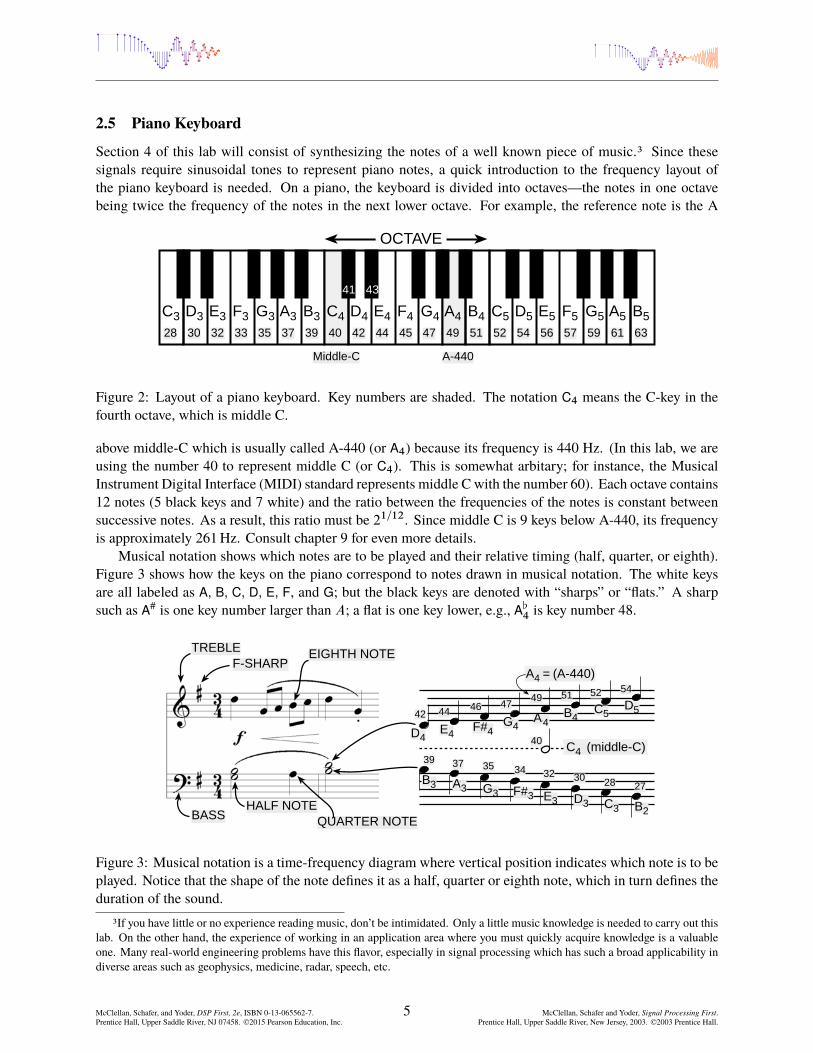
Section 4 of this lab will consist of synthesizing the notes of a well known piece of music.3 Since thesesignals require sinusoidal tones to represent piano notes, a quick introduction to the frequency layout ofthe piano keyboard is needed. On a piano, the keyboard is divided into octaves—the notes in one octavebeing twice the frequency of the notes in the next lower octave. For example, the reference note is the A
Figure 2: Layout of a piano keyboard. Key numbers are shaded. The notation C4 means the C-key in thefourth octave, which is middle C.
above middle-C which is usually called A-440 (or A4) because its frequency is 440 Hz. (In this lab, we areusing the number 40 to represent middle C (or C4). This is somewhat arbitary; for instance, the MusicalInstrument Digital Interface (MIDI) standard represents middle C with the number 60). Each octave contains12 notes (5 black keys and 7 white) and the ratio between the frequencies of the notes is constant betweensuccessive notes. As a result, this ratio must be 21=12. Since middle C is 9 keys below A-440, its frequencyis approximately 261Hz. Consult chapter 9 for even more details.
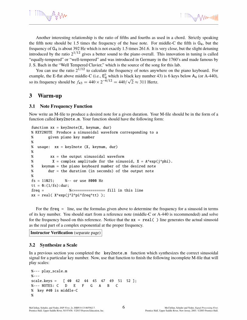
Musical notation shows which notes are to be played and their relative timing (half, quarter, or eighth).Figure 3 shows how the keys on the piano correspond to notes drawn in musical notation. The white keysare all labeled as A, B, C, D, E, F, and G; but the black keys are denoted with “sharps” or “flats.” A sharpsuch as A# is one key number larger than A; a flat is one key lower, e.g., A[
4 is key number 48.
A4 = (A-440)
TREBLE
BASS
F-SHARP
HALF NOTEQUARTER NOTE
EIGHTH NOTE
D5A4
C4 (middle-C)D4
E4F#4
G442 44 46 47
49
39 37 35 3430 28
32
40
51 52 54
C5
B3 A3 G3 F#3 E3 D3 C3 B2
27
B4
Figure 3: Musical notation is a time-frequency diagram where vertical position indicates which note is to beplayed. Notice that the shape of the note defines it as a half, quarter or eighth note, which in turn defines theduration of the sound.
3If you have little or no experience reading music, don’t be intimidated. Only a little music knowledge is needed to carry out thislab. On the other hand, the experience of working in an application area where you must quickly acquire knowledge is a valuableone. Many real-world engineering problems have this flavor, especially in signal processing which has such a broad applicability indiverse areas such as geophysics, medicine, radar, speech, etc.
Another interesting relationship is the ratio of fifths and fourths as used in a chord. Strictly speakingthe fifth note should be 1.5 times the frequency of the base note. For middle-C the fifth is G4, but thefrequency of G4 is about 392 Hz which is not exactly 1.5 times 261.6. It is very close, but the slight detuningintroduced by the ratio 21=12 gives a better sound to the piano overall. This innovation in tuning is called“equally-tempered” or “well-tempered” and was introduced in Germany in the 1760’s and made famous byJ. S. Bach in the “Well Tempered Clavier,” which is the source of the song for this lab.
You can use the ratio 21=12 to calculate the frequency of notes anywhere on the piano keyboard. Forexample, the E-flat above middle-C (i.e., E[
4 which is black key number 43) is 6 keys below A4 (or A-440),so its frequency should be f43 D 440 � 2
�6=12D 440=
p2 � 311 Hertz.
3 Warm-up
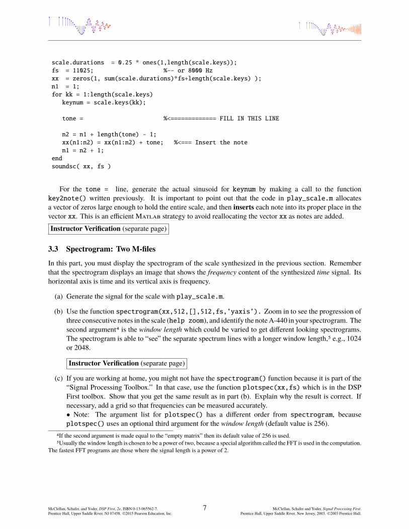
3.1 Note Frequency FunctionNow write an M-file to produce a desired note for a given duration. Your M-file should be in the form of afunction called key2note.m. Your function should have the following form:
function xx = key2note(X, keynum, dur)% KEY2NOTE Produce a sinusoidal waveform corresponding to a% given piano key number%% usage: xx = key2note (X, keynum, dur)%% xx = the output sinusoidal waveform% X = complex amplitude for the sinusoid, X = A*exp(j*phi).% keynum = the piano keyboard number of the desired note% dur = the duration (in seconds) of the output note%fs = 11025; %-- or use 8000 Hztt = 0:(1/fs):dur;freq = %<=============== fill in this linexx = real( X*exp(j*2*pi*freq*tt) );
For the freq = line, use the formulas given above to determine the frequency for a sinusoid in termsof its key number. You should start from a reference note (middle-C or A-440 is recommended) and solvefor the frequency based on this reference. Notice that the xx = real( ) line generates the actual sinusoidas the real part of a complex exponential at the proper frequency.
Instructor Verification (separate page)
3.2 Synthesize a ScaleIn a previous section you completed the key2note.m function which synthesizes the correct sinusoidalsignal for a particular key number. Now, use that function to finish the following incomplete M-file that willplay scales:
%--- play_scale.m%---scale.keys = [ 40 42 44 45 47 49 51 52 ];%--- NOTES: C D E F G A B C% key #40 is middle-C%
For the tone = line, generate the actual sinusoid for keynum by making a call to the functionkey2note() written previously. It is important to point out that the code in play_scale.m allocatesa vector of zeros large enough to hold the entire scale, and then inserts each note into its proper place in thevector xx. This is an efficient Matlab strategy to avoid reallocating the vector xx as notes are added.
Instructor Verification (separate page)
3.3 Spectrogram: Two M-files
In this part, you must display the spectrogram of the scale synthesized in the previous section. Rememberthat the spectrogram displays an image that shows the frequency content of the synthesized time signal. Itshorizontal axis is time and its vertical axis is frequency.
(a) Generate the signal for the scale with play_scale.m.
(b) Use the function spectrogram(xx,512,[],512,fs,’yaxis’). Zoom in to see the progression ofthree consecutive notes in the scale (help zoom), and identify the noteA-440 in your spectrogram. Thesecond argument4 is the window length which could be varied to get different looking spectrograms.The spectrogram is able to “see” the separate spectrum lines with a longer window length,5 e.g., 1024or 2048.
Instructor Verification (separate page)
(c) If you are working at home, you might not have the spectrogram() function because it is part of the“Signal Processing Toolbox.” In that case, use the function plotspec(xx,fs) which is in the DSPFirst toolbox. Show that you get the same result as in part (b). Explain why the result is correct. Ifnecessary, add a grid so that frequencies can be measured accurately.� Note: The argument list for plotspec() has a different order from spectrogram, becauseplotspec() uses an optional third argument for the window length (default value is 256).
4If the second argument is made equal to the “empty matrix” then its default value of 256 is used.5Usually the window length is chosen to be a power of two, because a special algorithm called the FFT is used in the computation.
The fastest FFT programs are those where the signal length is a power of 2.
The audible range of musical notes consists of well-defined frequencies assigned to each note in a musicalscore. Five different pieces are given in the book, but we have chosen a different one for the synthesis programin this lab. Before starting the project, make sure that you have a working knowledge of the relationshipbetween a musical score, key number and frequency. The following steps are an overview of the process ofactually synthesizing the music. Read it through, but don’t do it now. Rather we will walk you through eachstep in greater detail in the sections that follow.
(a) Determine a sampling frequency that will be used to play out the sound through the D-to-A system ofthe computer. This will dictate the time Ts between samples of the sinusoids.
(b) Determine the total time duration needed for each note, and also determine the frequency (in hertz)for each note (see Fig. 2 and the discussion of the well-tempered scale in the warm-up.) A data filecalled bach_fugue.mat is provided with this information stored in Matlab structures; this containsthe portion of the piece needed for this lab. A second file called bach_fugue_short.mat has thesame information for the first few measures of the piece; you may find this useful for initial debugging.Both of these files can be found in the zip file bach_fugueData.zip linked to the lab PDF.
(c) Synthesize the waveform as a combination of sinusoids, and play it out through the computer’s built-inspeaker or headphones using soundsc().
(d) Make a plot of a few periods of two or three of the sinusoids to illustrate that you have the correctfrequency (or period) for each note.
(e) Include a spectrogram image of a portion of your synthesized music—probably about 1 or 2 secs—sothat you can illustrate the fact that you have all the different notes. This piece has many sixteenthnotes, so a window length of 512 might be the best choice for spectrogram(). In addition, thespectrogram M-files will scale the frequency axis to run from zero to half the sampling frequency, soit might be useful to “zoom in” on the region where the notes are. Consult help zoom, or use thezoom tool in Matlab-v5.3 figure windows.
4.1 Spectrogram of the Music
Musical notation describes how a song is composed of different frequencies and when they should be played.This representation can be considered to be a time-frequency representation of the signal that synthesizes thesong. In Matlab we can can compute a time-frequency representation from the signal itself. This is calledthe spectrogram, and its implementation with the Matlab function spectrogram() or plotspec(). Toaid your understanding of music and its connection to frequency content, please refer to Chapter 3, Section3-6. This GUI also has the capability to synthesize music from a list of notes, but these notes are given in“standard” musical notation, not key number. For more information, consult the help on musicgui.m.
4.2 Fugue #2 for the Well-Tempered Clavier
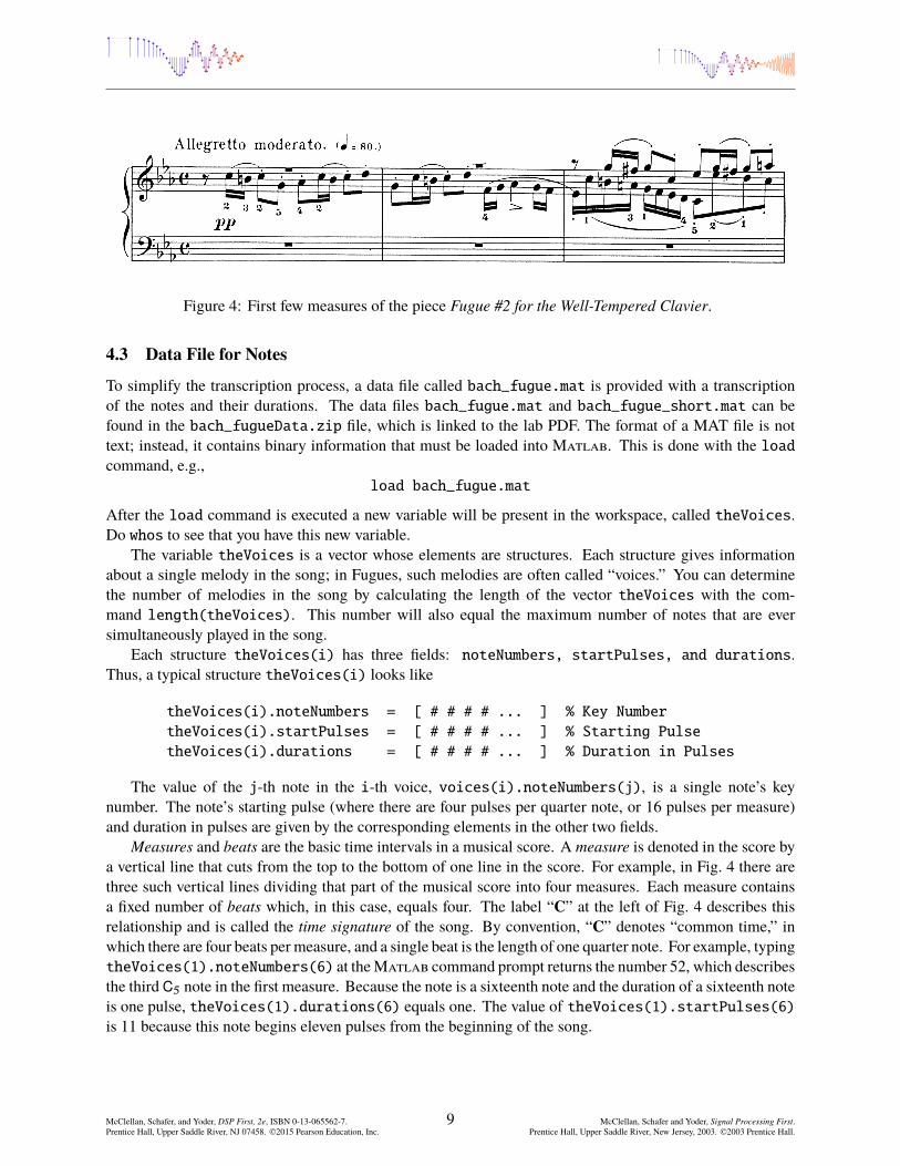
Fugue #2 for the Well-Tempered Clavier is one of those pieces of classical music that everyone has heard,but nobody particularly remembers its name. The first few measures are shown in Fig. 4.6 The goal ofthis lab is to synthesize the longer version of the Fugue #2 for the Well-Tempered Clavier given in the filebach_fugue.mat. Use sinusoids sampled at 11025 samples/s7 in your Matlab program.
6From a free sheet music site: https://www.pianoshelf.com/sheetmusic/729/bach-bwv-847---wtc,-book-1--prelude-and-fugue-no.-2-729 (Fugue starts on page 3).
7A lower sampling rate could be used if you have a computer with limited memory.
Figure 4: First few measures of the piece Fugue #2 for the Well-Tempered Clavier.
4.3 Data File for Notes
To simplify the transcription process, a data file called bach_fugue.mat is provided with a transcriptionof the notes and their durations. The data files bach_fugue.mat and bach_fugue_short.mat can befound in the bach_fugueData.zip file, which is linked to the lab PDF. The format of a MAT file is nottext; instead, it contains binary information that must be loaded into Matlab. This is done with the loadcommand, e.g.,
load bach_fugue.mat
After the load command is executed a new variable will be present in the workspace, called theVoices.Do whos to see that you have this new variable.
The variable theVoices is a vector whose elements are structures. Each structure gives informationabout a single melody in the song; in Fugues, such melodies are often called “voices.” You can determinethe number of melodies in the song by calculating the length of the vector theVoices with the com-mand length(theVoices). This number will also equal the maximum number of notes that are eversimultaneously played in the song.
Each structure theVoices(i) has three fields: noteNumbers, startPulses, and durations.Thus, a typical structure theVoices(i) looks like
The value of the j-th note in the i-th voice, voices(i).noteNumbers(j), is a single note’s keynumber. The note’s starting pulse (where there are four pulses per quarter note, or 16 pulses per measure)and duration in pulses are given by the corresponding elements in the other two fields.
Measures and beats are the basic time intervals in a musical score. A measure is denoted in the score bya vertical line that cuts from the top to the bottom of one line in the score. For example, in Fig. 4 there arethree such vertical lines dividing that part of the musical score into four measures. Each measure containsa fixed number of beats which, in this case, equals four. The label “C” at the left of Fig. 4 describes thisrelationship and is called the time signature of the song. By convention, “C” denotes “common time,” inwhich there are four beats per measure, and a single beat is the length of one quarter note. For example, typingtheVoices(1).noteNumbers(6) at theMatlab command prompt returns the number 52, which describesthe third C5 note in the first measure. Because the note is a sixteenth note and the duration of a sixteenth noteis one pulse, theVoices(1).durations(6) equals one. The value of theVoices(1).startPulses(6)is 11 because this note begins eleven pulses from the beginning of the song.
Musicians often think of the tempo, or speed of a song, in terms of “beats per minute” or BPM, where thebeats are usually quarter notes. You should write the code so that the BPM is a global parameter that can bechanged easily. For example, you might let the BPM be defined with the statement:
bpm = 120;
Computer programs which lets musicians record, modify, and play back notes played on a keyboard or otherelectronic instrument are called “sequencer.”8 The timing resolution of a sequencer is usually measured in“pulses per quarter note,” or PPQ. In this lab, we will employ four pulses per quarter note. A real commercialsequencer would have a much higher PPQ to encapsulate the subtle timing nuances of a real human playinga real instrument. The starting times and durations of notes in the music file provided to you are specified interms of “pulses,” so it will be helpful helpful to compute the number of “seconds per pulse,” via:
With a sixteenth note lasting one pulse, eighth notes are twice as long (2 pulses), and quarter notes fourtimes as long (4 pulses). If the tempo is defined only once, then it could be changed: for example, settingbpm = 240 would make the whole piece play twice as fast. Another timing issue is related to the fact thatwhen a musical instrument is played, the notes are not continuous. Therefore, inserting very short pausesbetween notes usually improves the musical sound because it imitates the natural transition that a musicianmust make from one note to the next. An envelope (discussed below) can accomplish the same thing.
4.4 Musical Tweaks
The all-sinusoids musical passage is likely to sound very artificial, when it is created from pure sinusoids.Therefore, you should try to improve the sound quality sound by incorporating some modifications. Forexample, one improvement comes from using an “envelope,” where you multiply each pure tone signal byan envelope E.t/ so that it fades in and out.
x.t/ D E.t/ cos.2�fkeyt C '/ (2)
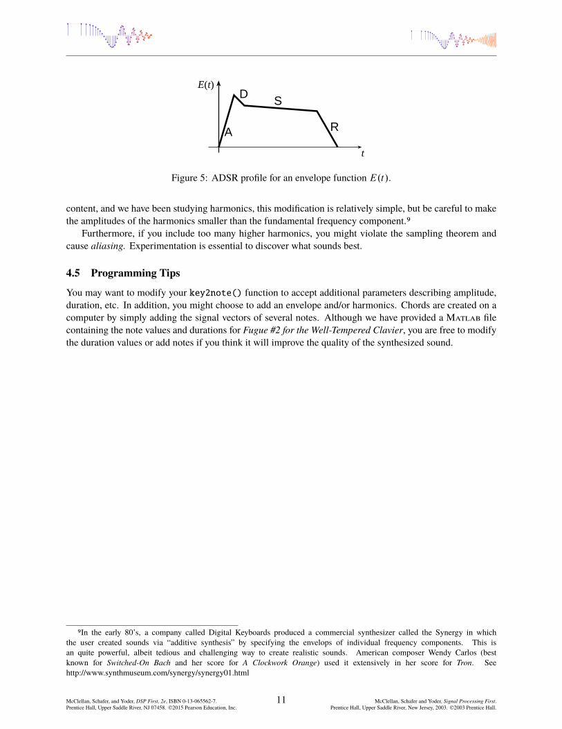
If an envelope is used, it should start quickly, i.e., “fade in”, and fade out more slowly. An envelope suchas a half-cycle of a sine wave sin.�t=dur/ is simple to program, but it sounds poor because it does notturn on quickly enough, so simultaneous notes of different durations no longer appear to begin at the sametime. A standard way to define the envelope function is to divide E.t/ into four sections: attack (A), delay(D), sustain (S), and release (R). Together these are called ADSR. The attack is a quickly rising front edge,the delay is a small short-duration drop, the sustain is more or less constant and the release drops quicklyback to zero. Figure 5 shows a linear approximation to the ADSR profile. Consult help on linspace() orinterp1() for functions that create linearly increasing and decreasing vectors.
Some other issues that affect the quality of your synthesis include relative timing of the notes, correctdurations for tempo, rests (pauses) in the appropriate places, relative amplitudes to emphasize certain notesand make others soft, and finally harmonics. Since true piano sounds have a second and third harmonic
8Popular commercial sequencers include Mark of the Unicorn’s Digital Performer, Emagic’s Logic Audio, Steinberg’s Cubaseand Opcode’s Studio Vision.
Figure 5: ADSR profile for an envelope function E.t/.
content, and we have been studying harmonics, this modification is relatively simple, but be careful to makethe amplitudes of the harmonics smaller than the fundamental frequency component.9
Furthermore, if you include too many higher harmonics, you might violate the sampling theorem andcause aliasing. Experimentation is essential to discover what sounds best.
4.5 Programming Tips
You may want to modify your key2note() function to accept additional parameters describing amplitude,duration, etc. In addition, you might choose to add an envelope and/or harmonics. Chords are created on acomputer by simply adding the signal vectors of several notes. Although we have provided a Matlab filecontaining the note values and durations for Fugue #2 for the Well-Tempered Clavier, you are free to modifythe duration values or add notes if you think it will improve the quality of the synthesized sound.
9In the early 80’s, a company called Digital Keyboards produced a commercial synthesizer called the Synergy in whichthe user created sounds via “additive synthesis” by specifying the envelops of individual frequency components. This isan quite powerful, albeit tedious and challenging way to create realistic sounds. American composer Wendy Carlos (bestknown for Switched-On Bach and her score for A Clockwork Orange) used it extensively in her score for Tron. Seehttp://www.synthmuseum.com/synergy/synergy01.html