DSP Implementation of a 1961 Fender Champ Amplifier by James Siegle

Advisor: Dr. Thomas L. Stewart EE 452 Senior Laboratory II

May 12, 2002

1

Table of Contents

Abstract .........................................................................................................................3

Introduction ..................................................................................................................4

Solid-State Amplifier Distortion ...................................................................................................4

Vacuum Tube Amplifier Distortion..............................................................................................5

Functional Description ................................................................................................6

Overview .........................................................................................................................................6

Inputs/Outputs................................................................................................................................6

Modes...............................................................................................................................................7

System Description.........................................................................................................................7

Design Equations and Calculations............................................................................9

1961 Fender Champ Data Analysis ..............................................................................................9 Time Domain Display...................................................................................................................9 Discrete Fourier Transform Computation for Amplifier Output ...............................................10

Frequency Point Size Selection .......................................................................................................................... 10 Magnitude Spectrum Computation..................................................................................................................... 10 Analog Frequency Display Computation ........................................................................................................... 10

Circuit Diagrams/PSPICE Simulations ...................................................................11

PSPICE Simulations of Vacuum Tube Amplifier Distortion...................................................11

1961 Fender Champ Schematic ..................................................................................................13

MATLAB Simulations/Analysis/Implementation...................................................14

Sinusoidal Frequency Selection...................................................................................................14

Verification of Highest Frequency Component from Guitar...................................................15

1961 Fender Champ Outputs from Sinusoidal Inputs..............................................................16

1961 Fender Champ Output from Guitar Input .......................................................................17

Nonlinear Transfer Characteristic Computations ....................................................................18

FIR Filter Designs ........................................................................................................................19

1961 Fender Champ DSP Model Simulation.............................................................................20

1961 Fender Champ DSP Model Implementation ....................................................................20

Conclusions .................................................................................................................23

Research ........................................................................................................................................23

Accomplishments..........................................................................................................................23

Patents and Standards ...............................................................................................24

2

Patents ...........................................................................................................................................24

Standards ......................................................................................................................................24

References ...................................................................................................................25

Appendix .....................................................................................................................26

Texas Instruments Embedded Target for TI C6000TM DSP Block and Code Build Configurations ..............................................................................................................................26

ADC and DAC Block Settings ....................................................................................................26 Simulation Parameters Settings .................................................................................................27

MATLAB Code ............................................................................................................................30 Champread.m – reads in 1961 Fender Champ Data from Sinusoidal Inputs............................30 Champtransfer.m – plots X-Y relationship between sinusoidal input and Champ output .........31 Champv2.m – final version of 1961 Fender Champ DSP Model Simulation ............................32 Table.m – sorts X-Y relationship between sinusoidal inputs and Champ outputs .....................38

1961 Fender Champ Model Executable Code from Embedded Target for TI C6000TM DSP in MATLAB 6.5 ............................................................................................................................40

3

Abstract Solid-state technology may dominate the present electronics world, but vacuum tubes continue to hold influence in the guitar amplifier industry. The sound of a guitar playing through a vintage vacuum tube amplifier has become a standard for most guitarists. Unlike solid-state guitar amplifiers, vacuum tube amplifiers produce specific, distorted guitar sounds. The quality and amount of harmonic distortion in overdriven vacuum tube guitar amplifiers has been found to be pleasing to several musicians. This desirable effect has been termed "tube distortion." Even though vacuum tube designs for guitar amplifiers are characterized by their superior sound, their disadvantages include high cost, fragility, limited availability of components, high waste heat generation, and manufacturing inconsistencies in the tubes. The objective of this project is to reproduce the distinct harmonic distortion of a 1961 Fender Champ with a low-cost DSP and thus implement a guitar amplifier with tube distortion without the bulky and awkward features of a tube amplifier. Once the DSP-based design is completed for this small amplifier, the algorithm can be reconfigured for other vintage vacuum tube amplifiers.

4

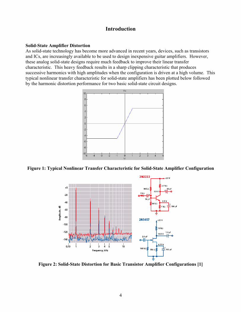
Introduction Solid-State Amplifier Distortion As solid-state technology has become more advanced in recent years, devices, such as transistors and ICs, are increasingly available to be used to design inexpensive guitar amplifiers. However, these analog solid-state designs require much feedback to improve their linear transfer characteristic. This heavy feedback results in a sharp clipping characteristic that produces successive harmonics with high amplitudes when the configuration is driven at a high volume. This typical nonlinear transfer characteristic for solid-state amplifiers has been plotted below followed by the harmonic distortion performance for two basic solid-state circuit designs.

Figure 1: Typical Nonlinear Transfer Characteristic for Solid-State Amplifier Configuration

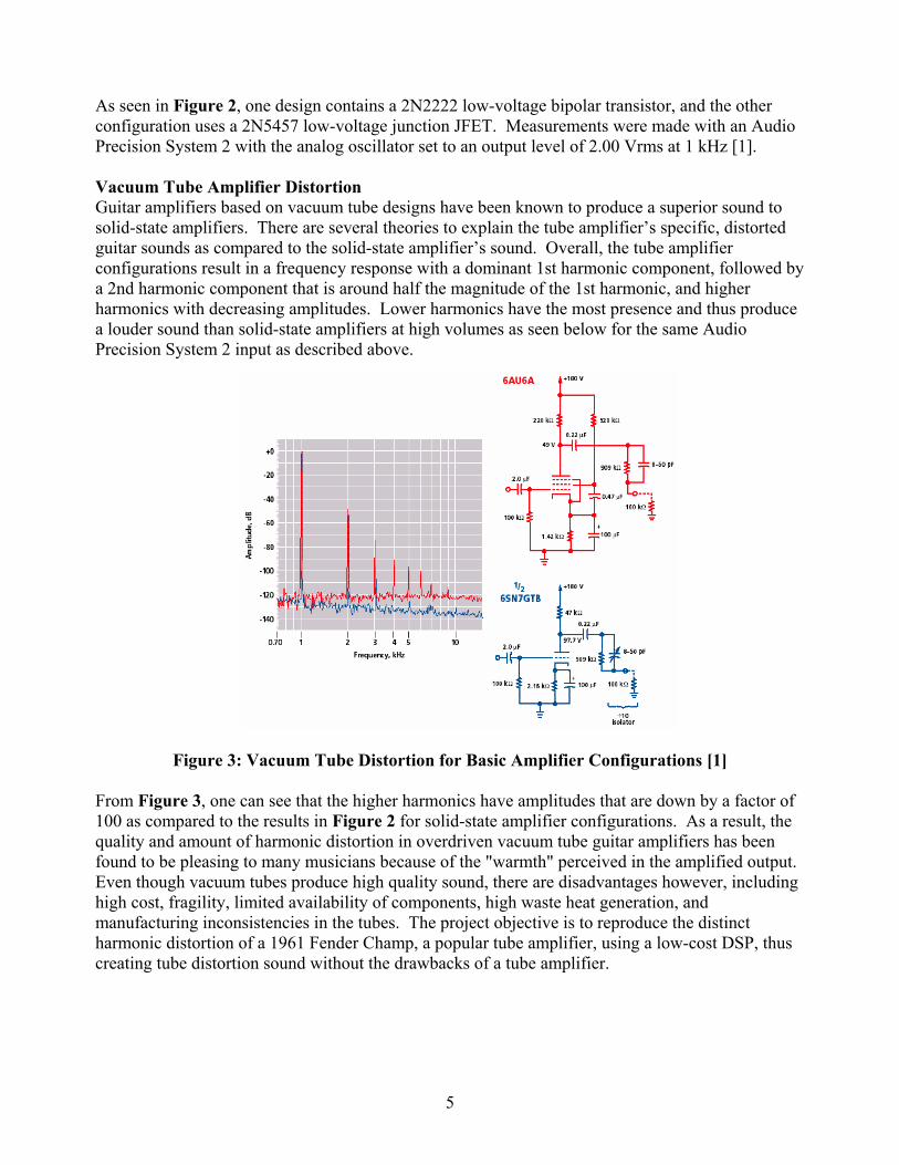
Figure 2: Solid-State Distortion for Basic Transistor Amplifier Configurations [1]

5

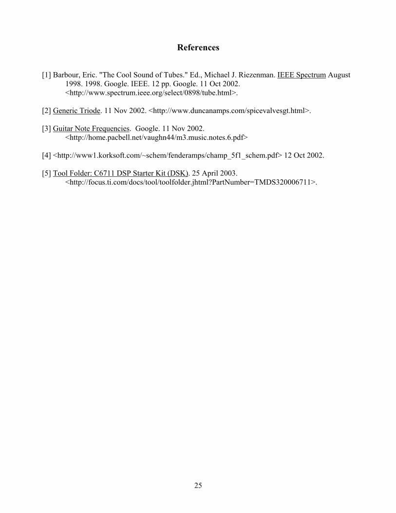
As seen in Figure 2, one design contains a 2N2222 low-voltage bipolar transistor, and the other configuration uses a 2N5457 low-voltage junction JFET. Measurements were made with an Audio Precision System 2 with the analog oscillator set to an output level of 2.00 Vrms at 1 kHz [1]. Vacuum Tube Amplifier Distortion Guitar amplifiers based on vacuum tube designs have been known to produce a superior sound to solid-state amplifiers. There are several theories to explain the tube amplifier’s specific, distorted guitar sounds as compared to the solid-state amplifier’s sound. Overall, the tube amplifier configurations result in a frequency response with a dominant 1st harmonic component, followed by a 2nd harmonic component that is around half the magnitude of the 1st harmonic, and higher harmonics with decreasing amplitudes. Lower harmonics have the most presence and thus produce a louder sound than solid-state amplifiers at high volumes as seen below for the same Audio Precision System 2 input as described above.

Figure 3: Vacuum Tube Distortion for Basic Amplifier Configurations [1]

From Figure 3, one can see that the higher harmonics have amplitudes that are down by a factor of 100 as compared to the results in Figure 2 for solid-state amplifier configurations. As a result, the quality and amount of harmonic distortion in overdriven vacuum tube guitar amplifiers has been found to be pleasing to many musicians because of the "warmth" perceived in the amplified output. Even though vacuum tubes produce high quality sound, there are disadvantages however, including high cost, fragility, limited availability of components, high waste heat generation, and manufacturing inconsistencies in the tubes. The project objective is to reproduce the distinct harmonic distortion of a 1961 Fender Champ, a popular tube amplifier, using a low-cost DSP, thus creating tube distortion sound without the drawbacks of a tube amplifier.

6

Functional Description Overview This project uses the Texas Instruments TMS320C6711, a 32-bit floating-point DSP seen below, to generate the transfer and distortion characteristics of a 1961 Fender Champ Amplifier at its 12 different volume settings. Audio signals generated by a guitar via an A/D interface to the DSP are passed through C/C++ digital filters with different gains. The averaged nonlinear transfer characteristic for each filter’s frequency range will reproduce the frequency response of the tube amplifier. Nonlinearities produced from this configuration are thought to be the primary reason for the improved quality of sound. The intention is to produce a vintage tube amplifier’s sound with a low-cost DSP as opposed to paying $1000 and up for a rare amplifier with limited replacement components.

Figure 4: Texas Instruments TMS320C6711 Evaluation DSP Board Layout [5]

Inputs/Outputs The system inputs are an analog audio signal from a guitar A/D interface, and a software based volume selection regulates the filters’ behavior. The output is an audio signal with similar effects to a tube amplifier. This signal is sounded with the D/A converter output that is interfaced to a set of 4”x 5” speakers equipped with a headphone connector. Both A/D and D/A converters are interfaced to standard headphone plug connectors. Therefore, only a 1/4” to 1/8” headphone plug was needed to interface the guitar to the board.

7

Modes The system modes consist of the volume settings similar to those provided with the 12-volume switch on the 1961 Fender Champ. The volume modeled for the amplifier was ‘6’ – the middle volume.

Figure 5: Overall Block Diagram

System Description The model consists of eight digital filters each cascaded with their own nonlinear transfer characteristic that was representative of the filters’ frequency ranges from the collected amplifier data. The output of each nonlinear model is filtered again to reduce any high frequency components that are not present from the 1961 Fender Champ data. The eight filtered results are then summed together and filtered once more by a bandpass filter with a wide passband to reduce any further high frequency terms from the summation operation and any DC offset. Each input sample is placed in memory after being collected on a frame basis and is processed on a sample-by-sample basis as each input becomes available from the external buffer. The result is a real-time filter with infinite duration once the DSP is initialized as shown in the software flow chart below.

Figure 6: Software Flowchart for DSP Model of 1961 Fender Champ

DSP with C/C++ Digital Filters

Analog Audio Signal from Guitar

Audio Output withTube Amplifier Sound

Interfacing Circuitryto Guitar Cable

Read inGuitar Input

Buffer InputData to 64

Samples/Frame

Filter Dataand Apply

Nonlinearity

Software Volume/Nonlinearity

Selection

Send out Equivalent

Amplifier Output

Y

N

Run (F5)

Shift+F5?

Halt

8

The digital filter banks were implemented with a 150-order FIR filter designs. If the algorithm’s noise floor is greater than the 16-bit input’s noise floor, the FIR model provides the best response. The figures below show the basic FIR filtering algorithm model, and the system block diagram respectively. Finally, all executable code for Texas Instruments eXpressDSPTM software was developed with MATLAB 6.5’s Embedded Target for the TI C6000TM DSP feature in Simulink®.

Figure 7: FIR Digital Filter Algorithm

Figure 8: Parallel FIR Filter Bank Approach to 1961 Fender Champ DSP Model

Analog Audio Signal Input from Guitar

Summer

Equivalent Tube AmplifierSignal Output

Mode of Operation (Software)

BP ...BP BP BP BP BP

Nonlinear Transfer Characteristics

BP ...BP BP BP BP BP

Final BP

9

Design Equations and Calculations 1961 Fender Champ Data Analysis Time Domain Display For the amplifier data analysis in MATLAB, the 1961 Fender Champ outputs were plotted in both the time and frequency domains. In order to view 4 periods of each output in the time domain the following relation was used N (Samples / period) = sampling frequency (Fs) (samples / sec) * ((1 / output frequency (F)) (sec /

period) Four times the resulting product was then entered into the right Limits text field under the X tab in the property editor window of MATLAB as shown below.

Figure 9: Samples/Period Entry in MATLAB for 1961 Fender Champ Data Plots

10

Discrete Fourier Transform Computation for Amplifier Output In order to display the magnitude spectrum for each of the 1961 Fender Champ outputs, the fft command in MATLAB was used to compute the Discrete Fourier Transform based on the following relation: N-1

X(k) = sum x(n)*e(-j*2*pi*(k)*(n)/N), 0 <= k <= N-1 n=0 The fft command in MATLAB is passed the variable storing the signal in the time domain and the number of frequency points to compute the Fourier Transform. This second parameter results in the computation of the Fast Fourier Transform. Frequency Point Size Selection For data with over 1 million points collected from the amplifier from a guitar input, the Fast Fourier Transform computation was preferred for its efficient results. The Fast Fourier Transform works most efficiently when the number of frequency points is a power of 2. For the amplifier outputs produced by sinusoidal inputs, the number of data points was between 80000 and 140000 thus calling for 2^17 (131072) or 2^18 (262144) frequency points in the second argument of the fft command. When amplifier data from a guitar input was plotted in the frequency domain, a power of 21 was used (2097152 frequency points). These frequency points were chosen to be the least power of two that resulted in the number of discrete frequency terms being greater than the number of time domain points. This way the fft computation was as efficient as possible while accounting for the periodic nature of the Discrete Fourier Transform and providing a higher resolution in the frequency component magnitudes. If later in the data analysis, the frequency components were shifted, the result would have zeros throughout the delay with the previous data appearing after the delay. Magnitude Spectrum Computation In order to plot the magnitude spectrum from the fft results, the absolute value was computed followed by a scaling factor of 2 divided by the number of data points in the time domain. When the data was recorded with the CoolEdit Software in the Acoustics Laboratory, the amplifier output was effectively turned on and then off as with a rectangular windowing function in the frequency domain. The frequency components' amplitudes are each multiplied by M (the number of data points) divided by 2 when this type of windowing is performed. This division is present to represent that the spectrum is double-sided. In order to view a single-sided magnitude spectrum with amplitudes representative of the amplifier data’s dynamic range, the absolute value of the fft results were properly scaled. Analog Frequency Display Computation Finally, to display the magnitude response data correctly versus continuous frequency values, each of the digital frequency terms, k, were scaled by the sampling frequency, Fs, divided by the number of frequency points, N. Since each frequency sample is (1/N) spaces apart from the fft computation, the analog frequency spacing from the computation is easily found by scaling the frequency samples by Fs/N. The MATLAB code to perform the computations discussed above and display the time domain and frequency domain content of the amplifier outputs can be found in the Appendix section under Champread.m.

11

Circuit Diagrams/PSPICE Simulations PSPICE Simulations of Vacuum Tube Amplifier Distortion Before beginning the development of the DSP model for the 1961 Fender Champ, some simulations of basic vacuum tube amplifier configurations were performed to verify the findings in Figure 3, to test the located vacuum tube PSPICE models, and to gain some insight into the source of vacuum tube amplifier’s unique distortion. First, PSPICE Transient Analysis simulations were completed for –20V to 60V sinusoidal inputs at 1 (kHz) for the 12AX7 triode. The schematic and simulation results can be seen below.

Figure 10: 12AX7 Triode PSPICE Transient Analysis Simulation Results

12

From the Figure 10 results, one can see that the first frequency component is dominant and all successive harmonics are much smaller when the amplifier is overdriven by the size of the input as in Figure 3. Overall, there is not much frequency content beyond the fifth harmonic component. The schematic and simulation results can be seen below for the 6V6GT amplifier and the same input specifications for the 12AX7 configuration were used as described on the previous page.

Figure 11: 6V6GT Pentode PSPICE Transient Analysis Simulation Results

From the results above, the output of the 6V6GT amplifier configuration consists of a dominant first harmonic component followed by higher frequency components with much smaller magnitudes. Again, there is not much frequency content beyond the fifth frequency component. However, the high harmonic amplitudes are much smaller than seen in Figure 3. This result is from the circuit configurations being different. Overall, both simulations show that the higher harmonics do not exhibit the behavior seen in Figure 2.

13

1961 Fender Champ Schematic The 1961 Fender Champ schematic drawn in PSPICE can be seen below. The 12AX7 and 6V6GT tube models were drawn and completed for this schematic and for Figure 10 and Figure 11 from the Duncan’s Amp Pages tutorial [2]. The original 1961 Fender Champ schematic was obtained from this site as well [4]. There was no data to be found on the 125A3A output transformer. All vacuum tube amplifier websites simply had vacuum tube data sheets and PSPICE ‘.inc’ files for a variety of vacuum tubes. Until the final component values can be found for the output transformer, the 1961 Fender Champ cannot be simulated, but is shown here since inputs were applied to this circuit to examine the amplifier output and model its nonlinear distortion.

Figure 12: 1961 Fender Champ (PSPICE) Schematic

14

MATLAB Simulations/Analysis/Implementation Sinusoidal Frequency Selection In order to develop the most accurate DSP model of the 1961 Fender Champ’s sound, several experiments had to be performed in the laboratory to gain a thorough understanding the amplifier’s behavior for various inputs. Most test inputs to the Champ were sinusoidal with the exception of one set of data taken from a 1952 Fender Telecaster. This data was later recorded directly from the guitar so that the DSP Model could be simulated with a MATLAB program. Frequencies chosen for the sinusoids were available from the guitar note frequency chart seen below [4].

Figure 13: Guitar Note Frequencies [3]

15

Verification of Highest Frequency Component from Guitar After collecting amplifier data from sinusoidal and guitar inputs, it was discovered that the Texas Instruments TMS320C6711 DSK board DSK uses a fixed clock rate of 150 MHz and has a fixed sampling frequency of 8 kHz on the A/D converter. This particular processor has been intended more for speech applications that only require around 4 kHz of bandwidth. Based on the data provided by Figure 13, it appeared that the last two notes on a standard 21-fret guitar would not be sounded properly due to aliasing. Therefore, the highest frequency from a guitar was verified by plugging the instrument into a 16-bit A/D converter configured for a 44.1 kHz sampling frequency and 16-bit stereo data collection. The sounds played through the guitar are then recorded in ‘.wav’ format with CoodEdit software. The first E string was plucked at the 21st fret of my guitar, and the time and frequency domain data were plotted below as discussed in the Design Equations section.

Figure 14: Highest Frequency Note from a 21-Fret Guitar

From the right plot above, one can see that there is a frequency component around 4434.92 (Hz) as indicated by Figure 13. However, the magnitude of this component is insignificant as compared to the other magnitudes produced by this note. Therefore, the conclusion was that not much information would be lost by prefiltering the guitar input within the 4 kHz range.

16

1961 Fender Champ Outputs from Sinusoidal Inputs Using the Figure 13 table as a reference, sinusoids at several frequencies were produced by a function generator and applied to the amplifier at volumes 3, 6, and 12. These volumes were picked to model since ‘3’ is the first audible volume, ‘6’ is the middle volume, and ‘12’ is the overdriven volume input where the amplifier exhibits its best distortion characteristics. The sound was recorded with a microphone connected to the 16-bit A/D converter configured for the settings discussed above. With this setup, all of the data in the recording takes into account all the components of the amplifier including the speaker and the transformer. The outputs were plotted in the format shown below based on the Design Equations discussion and the MATLAB code attached in the Appendix in Champread.m.

Figure 15: 523.25 (Hz) Sinusoidal Input (Top),

1961 Fender Champ Output and Magnitude Response (Bottom)

17

1961 Fender Champ Output from Guitar Input After all sinusoidal data was collected, a guitar input containing high and low frequency components was applied to the amplifier set at volume 6 and recorded in a similar procedure discussed in the previous section. The note sequence was played again with the guitar connected directly to A/D converter. Below are the MATLAB plots of the response in the time domain and the frequency domain.

Figure 16: Input to 1961 Fender Champ at Volume ‘6’

(Output of Guitar – 1952 Fender Telecaster)

Figure 17: Fender Champ Response at Volume ‘6’ to Figure 16

The results in Figure 16 were then applied to the MATLAB simulation of the DSP amplifier model. The output of this model could be compared to Figure 17, in addition to sounding the result, in order to verify the model’s accuracy in matching the Champ’s unique distortion.

18

Nonlinear Transfer Characteristic Computations To model the nonlinear distortion of the 1961 Fender Champ at different frequencies, an X-Y relationship needed to be established between the sinusoidal inputs and their corresponding outputs. In order to conserve the DSP board’s memory, equation fits for the nonlinear transfer characteristics were performed iteratively with the polyfit command in MATLAB. Also, the nonlinearity for each sinusoidal frequency was broken up into two parts since the output differed on the decreasing side of the input as compared to the increasing portion of the input. The points were grouped by first matching their zero crossing point. Two separate plots were produced for the increasing side of the sinusoid and the decreasing side of the sinusoid. The MATLAB code to generate these plots is included in the Appendix in Champtransfer.m. Polynomial fits of orders 3, 4, and 5 were performed on the curves at random increments of the sinusoidal points on the command line. The resulting polynomials for the eight selected frequencies in Figure 8 can be found in the final MATLAB simulation code for the DSP amplifier model in the Appendix in Champv2.m. Below are the nonlinear transfer characteristic curves for Figure 15.

Figure 18: Nonlinear Transfer Characteristics for Figure 15

From the similarities and differences between these nonlinear transfer characteristic curves, certain nonlinearities were selected to be representative of certain frequency ranges as listed in the table below.

Frequency Range (Hz) Nonlinear Transfer Characteristic Frequency (Hz) 250- 450 329.63 450-700 523.25 700-900 783.99 900-1200 1046.50 1200-1500 1318.51 1500-2000 1760.00 2000-3000 2637.02 3000-4000 4434.92

Table 1: Nonlinear Transfer Characteristic Curve Definitions for DSP Amplifier Model

19

FIR Filter Designs Since a significant amount of time was spent fitting the nonlinear transfer characteristic curves for all the sinusoidal frequencies applied to the 1961 Fender Champ, the Filter Design and Analysis Tool (FDATool), under the Signal Processing Toolbox in MATLAB, was used to design the FIR filters used in the DSP amplifier model as shown below.

Figure 19: Filter Design and Analysis Tool (FDATool) in MATLAB

From the figure above, a filter design’s magnitude and phase response can be viewed after specifying the cutoff frequency, sampling frequency, windowing function, filter order, and filter type in the appropriate text fields. FIR filter orders were 2000 for the MATLAB code simulation of the DSP amplifier model due to the 44.1 kHz sampling frequency that was used to collect the Champ output data and the sharp cutoffs required by the filters in order to prevent amplifying the signal out of the –1 to 1 range for the nonlinear transfer characteristic equations. When the design would later be implemented on the TMS320C6711 DSK board with an 8 kHz sampling frequency, the FIR filter orders could be reduced to an order below 200.

20

1961 Fender Champ DSP Model Simulation After correcting several nonlinear transfer characteristic curve fits and correcting several decision case statements in the MATLAB code simulation of the amplifier’s DSP model in Figure 8, the final result was produced below.

Figure 20: MATLAB Code Simulation of DSP Model for Volume 6 of 1961 Fender Champ

From the results above, the output is bounded within the –0.6 to 0.6 amplitude range as in Figure 17. Differences between the waves, noticeable around the 60000th sample, are partially due to the fact that both sets of data were not played exactly the same. The frequency spectrum matches the response in Figure 17 with the exception of the removal of the frequency components in the DC range of 0-250 Hz and the range beyond 4500 (Hz). When the DC range was included in the model, a significant amount of noise was produced in this range that in turn masked out the sound. The Figure 8 model generated high frequency components greater than 10 kHz since the nonlinear transfer characteristic curves were defined for single frequency inputs, and not a range of frequencies. To alleviate this problem, the output from each of the eight nonlinear transfer characteristic curves was filtered again to reduce high frequency content. Using the sound command in MATLAB, the output still did not quite match the output of Figure 17, but there were several similarities leaving the model to be implemented on the Texas Instruments DSP board. 1961 Fender Champ DSP Model Implementation In order to implement the DSP amplifier model on the Texas Instruments DSP board, there is a feature in MATLAB 6.5 that allows a DSP-based Simulink model to be translated to ANSI C standard code to be executable in the Texas Instruments Code Composer Studio (CCS) development software for a selection of Texas Instruments DSP developer boards. This feature is the Embedded Target for the Texas Instruments C6000TM DSP. This embedded target supports the TMS320C6711 DSK board available for the project as shown by the blockset figure on the next page.

21

Figure 21: Texas Instruments TMS320C6711 Blockset Support from MATLAB 6.5’s

Embedded Target for TI C6000TM DSP The blocks of interest above to implement the Figure 8 design are the ADC, DAC, and the Reset Blocks. Reset simply allows the user to reset the board to the original register and memory settings from the Simulink model window. ADC and DAC enable the board to accept external signals from the A/D converter and send signals out through the D/A converter respectively. The Embedded Target settings for these blocks and code generation and execution are more thoroughly explained on pages 26-29 of the Appendix. The Simulink block diagram of Figure 8 can be seen below.

Figure 22: Simulink Implementation of 1961 Fender Champ DSP Model

22

From Figure 22, the nonlinear transfer characteristic equations have been replaced with lookup tables since the S-function blocks in MATLAB 6.5 resulted in a build failure for the DSP board. These blocks allow piecewise polynomial formula entries needed for the nonlinear transfer characteristics listed in Table 1. The MATLAB help files indicated that the Embedded Target feature is only defined for the DSP Blockset in Simulink and a few other blocks including the Look-Up Table block. These look-up tables were generated by sorting the sinusoidal values in monotonically increasing fashion for the nonlinear transfer characteristic curves. The corresponding amplifier outputs were also sorted. MATLAB code to perform this sorting procedure can be found in Table.m in the Appendix. The sorted version of Figure 18 can be seen below.

Figure 23: Sorted Nonlinear Transfer Characteristic for Figure 18

The above curve is similar to the preview curves generated Figure 22’s Look-Up Table blocks. Once the FIR filter orders from the FDATool were reduced to 150 for the parallel filter bank, and the input and output filter orders were reduced to 50, the TMS320C6711 was effectively programmed and 1961 Fender Champ DSP model was ready for demonstration. The output of the speakers was clean and loud for lower frequency notes on the guitar. For higher frequency notes, a harsh sound was generated when the gain from the guitar was set to its highest position. The source of this harsh sound may be the equivalent high frequency sound heard in the MATLAB simulations from Figure 20. The real-time DSP Blockset sink scopes have not been enabled correctly to obtain any real-time data from the board to be analyzed later in the time and frequency domains. However, the overall sound was similar to the 1961 Fender Champ’s sound in Figure 17.

23

Conclusions Research Further research or improvements in the design that have been considered are locating the 1961 Fender Champ’s transformer data so that the circuit in Figure 12 can be simulated in PSPICE. The simulation results can then be used to establish an X-Y relationship between the input and output of the amplifier for a wider frequency range and for all 12 volumes. This approach would result in simpler design. Also, the design can be implemented with a 12-state subband coding structure that would divide the 4 kHz bandwidth input from the guitar into ~1 Hz frequency ranges. Each nonlinearity can then be applied to single frequencies resulting in an improved sound. This design will be more efficient since all the lowpass and highpass filters in the subband coding structure are the same. Finally, an investigation into the source of the Embedded Target’s code generation capabilities should be completed to have an appreciation of MATLAB 6.5’s new powerful feature. Accomplishments Overall, the project was successful in implementing the DSP-based 1961 Fender Champ amplifier on the Texas Instruments TMS320C6711 DSK board for one volume setting. Only designs with little complexity have been produced for past DSP boards. In general, DSP boards are difficult to program as a result of poor accompanying documentation and unclear external peripheral layouts. This project’s model was complex and implemented on a DSP evaluation board in less than a week. MATLAB 6.5’s Embedded Target for the TI C6000TM feature is a powerful tool for implementing DSP-based designs without the time-consuming programming task.

24

Patents and Standards Patents Two patents have the same objective as this project, but both DSP algorithms do not involve any of the approaches discussed in the Functional Description section. Also, neither patent intends to specifically model the 1961 Fender Champ. The patents are listed below.

• Tube Modeling Programmable Digital Guitar Amplification System • U.S. Patent 5,789,689 – August 4, 1998 • Employs a sampling rate conversion algorithm to model the nonlinear transfer function

of the tube circuitry.

• Electric instrument amplifier • U.S. Patent 6,350,943 – February 26, 2002 • Employs a sampling rate conversion algorithm to model the nonlinear transfer function

of the tube circuitry. • Includes a tube configuration and a solid-state power circuit on the D/A output of the

DSP board.

Figure 24: Patent Vacuum Tube Amplifier DSP Modeling Algorithm

Standards N/A

Nonlinearity Filter Result forDownsampling Upsample Linear Interpolation Downsample

25

References [1] Barbour, Eric. "The Cool Sound of Tubes." Ed., Michael J. Riezenman. IEEE Spectrum August

1998. 1998. Google. IEEE. 12 pp. Google. 11 Oct 2002. <http://www.spectrum.ieee.org/select/0898/tube.html>.

[2] Generic Triode. 11 Nov 2002. <http://www.duncanamps.com/spicevalvesgt.html>. [3] Guitar Note Frequencies. Google. 11 Nov 2002.

<http://home.pacbell.net/vaughn44/m3.music.notes.6.pdf> [4] <http://www1.korksoft.com/~schem/fenderamps/champ_5f1_schem.pdf> 12 Oct 2002. [5] Tool Folder: C6711 DSP Starter Kit (DSK). 25 April 2003.

<http://focus.ti.com/docs/tool/toolfolder.jhtml?PartNumber=TMDS320006711>.

26

Appendix

Texas Instruments Embedded Target for TI C6000TM DSP Block and Code Build Configurations

ADC and DAC Block Settings The ADC block in Simulink for the Texas Instruments Embedded Target was configured as shown below to successfully produce the equivalent amplifier sound from the guitar.

Figure 25: C6711 DSK ADC Block Settings for 1961 Fender Champ DSP Model As seen above, in order to process data from a microphone or guitar input, the ‘ADC source’ text field must be set to “Mic In,” and the +20dB Mic gain boost must be enable to pick up the small amplitude signals from the guitar. All other settings are default values. The DAC block for the Texas Instruments Embedded Target was configured as shown below to its default settings.

Figure 26: C6711 DSK DAC Block Settings for 1961 Fender Champ DSP Model

27

Simulation Parameters Settings

Figure 27: C6711 DSK Simulation Parameters Settings for 1961 Fender Champ DSP Model

28

Figure 28: Figure 27, contd.

29

As seen in Figure 27 and Figure 28, most of the settings are disabled once the C6711 is selected in the ‘Target Selection’ window. The most important windows are at the bottom of Figure 28. The ‘TI C6000 code generation’ options allow the user’s code to have a high speed of execution by regenerating code for repeating blocks in their design, or generating code once for the repeating structure. The default setting is ‘Inline DSP Blockset functions’ that generates the repetitive code. For applications where conserving memory is an issue, the ‘target specific optimization’ option may need to be enabled. However, this alternative option does result in computation errors (LSB differences) as indicated in Figure 28. The ‘TI C6000 runtime’ options allow the user to only generate code, build the project, create a project, or build and execute the project. In the “Overrun action” field, the user can be warned that a board overrun has occurred by lighting an LED on the board with the ‘Continue’ selection; the program can be stopped at a board overrun with the ‘Halt’ selection; or the program can continue running despite the overrun with ‘None’ selection. As seen in Figure 28, ‘None’ was selected for the project implementation and no problems occurred, but future users of the Embedded Target feature in MATLAB 6.5 may want to consider a different setting. All other settings are self-explanatory from their description, and documentation on these settings can be easily found in the Embedded Target for Texas Instruments C6000 DSP’s help branch in the MATLAB 6.5 help files.

30

MATLAB Code Champread.m – reads in 1961 Fender Champ Data from Sinusoidal Inputs % MATLAB '.wav' Reading Code to Plot Frequency Response Data % from Sinusoidal Inputs to the 1961 Fender Champ clear all; Fs = 44100; % sampling frequency of recorded 16-bit precision data from amplifier [m] = wavread ('james12.wav'); % load 16-bit 44.1 (kHz) Fender Champ output samples in time domain % determine power of two frequency samples to take to avoid aliasing and ensure high frequency resolution N = 2^17; % initially set number of frequency samples to 131072 since % most of the data has 105986 or less elements if ((size (m, 1) > N)) % if power of 2 is less than size of Fender Champ output data N = 2^18; % N must be increased by a factor of 2 else N = 2^17; % N = # of frequency samples in FFT end % compute FFT of input wave data from Fender Champ and equivalent analog frequency terms % from DFT dependent variable 'k' mf = fft (m, N); % take the FFT of the sampled Fender Champ output mfmag = 2/(size (m, 1))*abs (mf); % calculate magnitude frequency response, |Y(F)|, of Fender Champ output mfmagdB = 20*log10(mfmag); % compute magnitude frequency response of Fender Champ output in 'dB' k = 1:1:N; % array of frequency sample integer points F = (Fs / N) * k; % conversion from array of frequency sample point, 'k', to analog frequency, 'F' % plot Fender Champ output vs. 'n' figure(2), plot(m), xlabel('n'), ylabel('Vo(n)'), title ('1961 Fender Champ Output from 523.25 (Hz) Sinusoidal Input') % plot magnitude response of Fender Champ output vs. frequency figure (3), plot (F, mfmag), title ('Magnitude Response of 1961 Fender Champ (Volume 12) to 1Vp 523.25 (Hz) Sinusoidal Input'), xlabel ('F'), ylabel ('|Vo(f)|'), axis([0 10000 0 0.5])

31

Champtransfer.m – plots X-Y relationship between sinusoidal input and Champ output % MATLAB code to generate the input-output transfer characteristic % of the 1961 Fender Champ for both the decreasing and increasing % portions of the sinusoidal input and corresponding output clear all; % load 16-bit 44.1 (kHz) Fender Champ output samples in time domain [m] = wavread ('james12.wav'); % sinusoidal input to 1961 Fender Champ A = 1; % 1Vp amplitude F = 523.25; % input frequency Fs = 44100; % sampling frequency n = 1:1:(size(m,1)); % number of samples in the output x = A*cos (2*pi*n*F/Fs); % sinusoidal input to the amplifier n = Fs / F; % number of samples per period in the input and output n = round(round (n) / 2); % round the above computation and divide by 2 (samples in negative to positive swing) x = x(n:(2*n)); % limit input value range to negative and positive peaks of the wave % initialize negative and positive peak indexes from amplifier output M = size (m, 1); % recalculate number of samples from amplifier output indexlower = 0; % set index of negative output peak to 0 indexhigher = 0; % set index of positive output peak to 0 % loop to find negative and positive peaks of amplifier output i = 1; % initialize loop count to 1 while (i <= M & indexlower == 0 & indexhigher == 0), % while loop count is less than output size and no range % has been found for output negative to positive peaks if (m(i,2) < 0 & m(i+1,2) >= 0 & (i-(n/2)) > 0 & m(i+4,2) > 0.4) % if the current output is less than zero, later sample % output values are greater than or equal to 0, and there are % '(1/4)*output period' values for the negative output portion indexhigher = round (i + (n/2)); % store location of rising portion of output to positive peak indexlower = round(i - (n/2)); % store location of rising portion following negative peak else end i = i + 1; % increment loop count end % increment 'indexlower' index if 'indexlower' to 'indexhigher' will result in % the output array ('y1') being one element larger than the sinusoidal input ('x') if ((indexhigher - indexlower) == size (x,2)) indexlower = indexlower + 1; else end % transfer half the period of the output of the amplifier to 'y1' y1 = m (indexlower:indexhigher, 2); % the amplifier output containing the negative and positive peaks y1 = transpose (y1); % transpose 'y1' so it has the same dimensions as the input 'x % determine transfer characteristic on decreasing wave portion before negative and after positive peaks indexlower = round (indexhigher + n); % set 'indexlower' to higher sample value than 'indexhigher' for % transfer characteristic determination of the output's decreasing side % (other half of one period of the output) if ((indexlower - indexhigher) == size (x,2)) % decrement 'indexlower' index if 'indexlower' to 'indexhigher' will result in indexlower = indexlower - 1; % the output array ('y1') being one element larger than the sinusoidal input ('x') else end i = indexlower; % set 'i' index to 'indexlower' (higher index for special case) j = 1; % set 'j' index variable to 1 while (i <= indexlower & i >= indexhigher), % loop from higher index value (negative peak) to lower index value (positive peak) y(j) = m(i,2); % and assign the appropriate values of the amplifier output j = j + 1; % increment 'y' assignment index i = i - 1; % decrement 'm' assignment index end % plot input(x)-output(y1) transfer characteristic for increasing negative peak to positive peak of the output figure (3), plot(x,y1), title ('1961 Fender Champ (Volume 6) Positive Input-Output Transfer Characteristic for 1Vp 523.25 (Hz) Sinusoidal Input'), xlabel ('input x(n)'), ylabel ('output y(n)') % plot input(x)-output(y1) transfer characteristic for decreasing negative peak to positive peak of the output figure (4), plot(x,y), title ('1961 Fender Champ (Volume 6) Negative Input-Output Transfer Characteristic for 1Vp 523.25 (Hz) Sinusoidal Input'), xlabel ('input x(n)'), ylabel ('output y(n)')

32

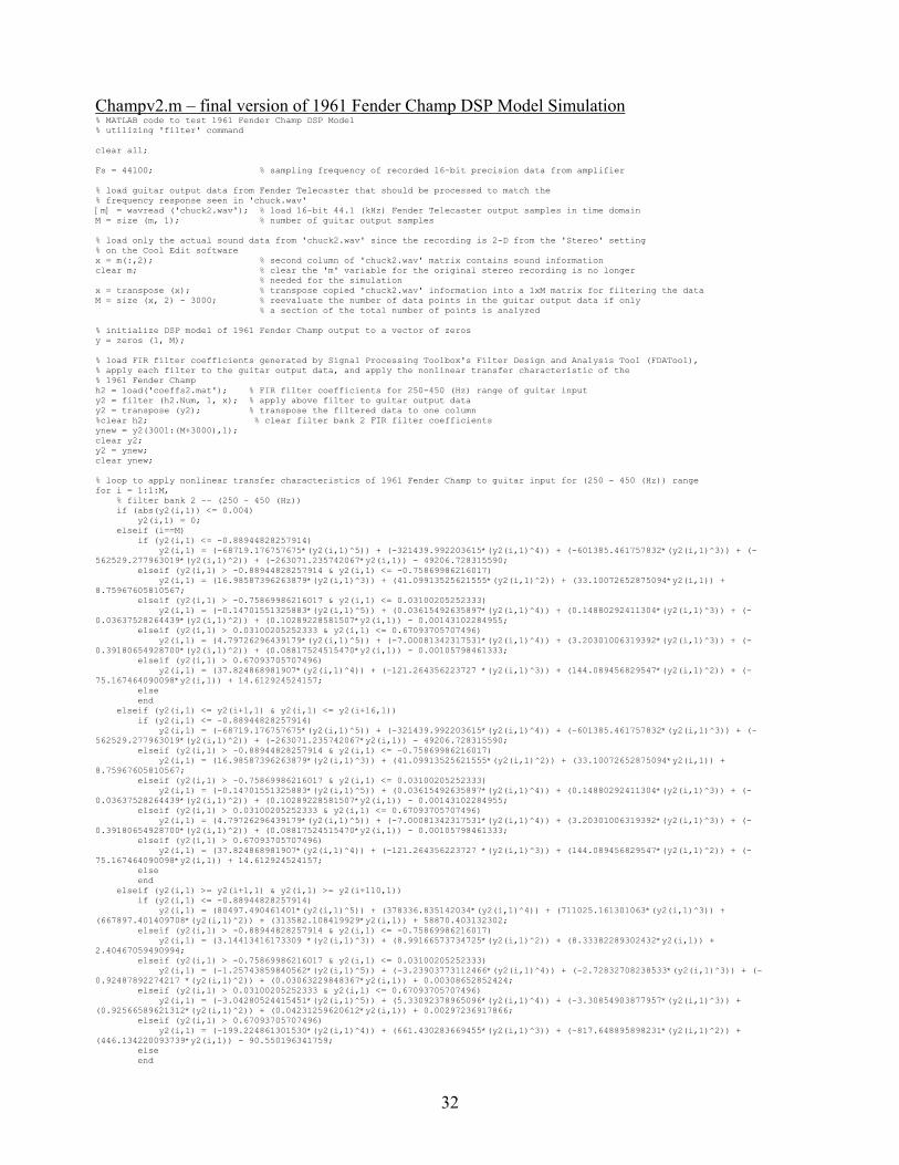
Champv2.m – final version of 1961 Fender Champ DSP Model Simulation % MATLAB code to test 1961 Fender Champ DSP Model % utilizing 'filter' command clear all; Fs = 44100; % sampling frequency of recorded 16-bit precision data from amplifier % load guitar output data from Fender Telecaster that should be processed to match the % frequency response seen in 'chuck.wav' [m] = wavread ('chuck2.wav'); % load 16-bit 44.1 (kHz) Fender Telecaster output samples in time domain M = size (m, 1); % number of guitar output samples % load only the actual sound data from 'chuck2.wav' since the recording is 2-D from the 'Stereo' setting % on the Cool Edit software x = m(:,2); % second column of 'chuck2.wav' matrix contains sound information clear m; % clear the 'm' variable for the original stereo recording is no longer % needed for the simulation x = transpose (x); % transpose copied 'chuck2.wav' information into a 1xM matrix for filtering the data M = size (x, 2) - 3000; % reevaluate the number of data points in the guitar output data if only % a section of the total number of points is analyzed % initialize DSP model of 1961 Fender Champ output to a vector of zeros y = zeros (1, M); % load FIR filter coefficients generated by Signal Processing Toolbox's Filter Design and Analysis Tool (FDATool), % apply each filter to the guitar output data, and apply the nonlinear transfer characteristic of the % 1961 Fender Champ h2 = load('coeffs2.mat'); % FIR filter coefficients for 250-450 (Hz) range of guitar input y2 = filter (h2.Num, 1, x); % apply above filter to guitar output data y2 = transpose (y2); % transpose the filtered data to one column %clear h2; % clear filter bank 2 FIR filter coefficients ynew = y2(3001:(M+3000),1); clear y2; y2 = ynew; clear ynew; % loop to apply nonlinear transfer characteristics of 1961 Fender Champ to guitar input for (250 - 450 (Hz)) range for i = 1:1:M, % filter bank 2 -- (250 - 450 (Hz)) if (abs(y2(i,1)) <= 0.004) y2(i,1) = 0; elseif (i==M) if (y2(i,1) <= -0.88944828257914) y2(i,1) = (-68719.176757675*(y2(i,1)^5)) + (-321439.992203615*(y2(i,1)^4)) + (-601385.461757832*(y2(i,1)^3)) + (-562529.277963019*(y2(i,1)^2)) + (-263071.235742067*y2(i,1)) - 49206.728315590; elseif (y2(i,1) > -0.88944828257914 & y2(i,1) <= -0.75869986216017) y2(i,1) = (16.98587396263879*(y2(i,1)^3)) + (41.09913525621555*(y2(i,1)^2)) + (33.10072652875094*y2(i,1)) + 8.75967605810567; elseif (y2(i,1) > -0.75869986216017 & y2(i,1) <= 0.03100205252333) y2(i,1) = (-0.14701551325883*(y2(i,1)^5)) + (0.03615492635897*(y2(i,1)^4)) + (0.14880292411304*(y2(i,1)^3)) + (-0.03637528264439*(y2(i,1)^2)) + (0.10289228581507*y2(i,1)) - 0.00143102284955; elseif (y2(i,1) > 0.03100205252333 & y2(i,1) <= 0.67093705707496) y2(i,1) = (4.79726296439179*(y2(i,1)^5)) + (-7.00081342317531*(y2(i,1)^4)) + (3.20301006319392*(y2(i,1)^3)) + (-0.39180654928700*(y2(i,1)^2)) + (0.08817524515470*y2(i,1)) - 0.00105798461333; elseif (y2(i,1) > 0.67093705707496) y2(i,1) = (37.824868981907*(y2(i,1)^4)) + (-121.264356223727 *(y2(i,1)^3)) + (144.089456829547*(y2(i,1)^2)) + (-75.167464090098*y2(i,1)) + 14.612924524157; else end elseif (y2(i,1) <= y2(i+1,1) & y2(i,1) <= y2(i+16,1)) if (y2(i,1) <= -0.88944828257914) y2(i,1) = (-68719.176757675*(y2(i,1)^5)) + (-321439.992203615*(y2(i,1)^4)) + (-601385.461757832*(y2(i,1)^3)) + (-562529.277963019*(y2(i,1)^2)) + (-263071.235742067*y2(i,1)) - 49206.728315590; elseif (y2(i,1) > -0.88944828257914 & y2(i,1) <= -0.75869986216017) y2(i,1) = (16.98587396263879*(y2(i,1)^3)) + (41.09913525621555*(y2(i,1)^2)) + (33.10072652875094*y2(i,1)) + 8.75967605810567; elseif (y2(i,1) > -0.75869986216017 & y2(i,1) <= 0.03100205252333) y2(i,1) = (-0.14701551325883*(y2(i,1)^5)) + (0.03615492635897*(y2(i,1)^4)) + (0.14880292411304*(y2(i,1)^3)) + (-0.03637528264439*(y2(i,1)^2)) + (0.10289228581507*y2(i,1)) - 0.00143102284955; elseif (y2(i,1) > 0.03100205252333 & y2(i,1) <= 0.67093705707496) y2(i,1) = (4.79726296439179*(y2(i,1)^5)) + (-7.00081342317531*(y2(i,1)^4)) + (3.20301006319392*(y2(i,1)^3)) + (-0.39180654928700*(y2(i,1)^2)) + (0.08817524515470*y2(i,1)) - 0.00105798461333; elseif (y2(i,1) > 0.67093705707496) y2(i,1) = (37.824868981907*(y2(i,1)^4)) + (-121.264356223727 *(y2(i,1)^3)) + (144.089456829547*(y2(i,1)^2)) + (-75.167464090098*y2(i,1)) + 14.612924524157; else end elseif (y2(i,1) >= y2(i+1,1) & y2(i,1) >= y2(i+110,1)) if (y2(i,1) <= -0.88944828257914) y2(i,1) = (80497.490461401*(y2(i,1)^5)) + (378336.835142034*(y2(i,1)^4)) + (711025.161301063*(y2(i,1)^3)) + (667897.401409708*(y2(i,1)^2)) + (313582.108419929*y2(i,1)) + 58870.403132302; elseif (y2(i,1) > -0.88944828257914 & y2(i,1) <= -0.75869986216017) y2(i,1) = (3.14413416173309 *(y2(i,1)^3)) + (8.99166573734725*(y2(i,1)^2)) + (8.33382289302432*y2(i,1)) + 2.40467059490994; elseif (y2(i,1) > -0.75869986216017 & y2(i,1) <= 0.03100205252333) y2(i,1) = (-1.25743859840562*(y2(i,1)^5)) + (-3.23903773112466*(y2(i,1)^4)) + (-2.72832708238533*(y2(i,1)^3)) + (-0.92487892274217 *(y2(i,1)^2)) + (0.03063229848367*y2(i,1)) + 0.00308652852424; elseif (y2(i,1) > 0.03100205252333 & y2(i,1) <= 0.67093705707496) y2(i,1) = (-3.04280524415451*(y2(i,1)^5)) + (5.33092378965096*(y2(i,1)^4)) + (-3.30854903877957*(y2(i,1)^3)) + (0.92566589621312*(y2(i,1)^2)) + (0.04231259620612*y2(i,1)) + 0.00297236917866; elseif (y2(i,1) > 0.67093705707496) y2(i,1) = (-199.224861301530*(y2(i,1)^4)) + (661.430283669455*(y2(i,1)^3)) + (-817.648895898231*(y2(i,1)^2)) + (446.134220093739*y2(i,1)) - 90.550196341759; else end

33

else end end % clear filter coefficients for 2nd filter bank, add the result to the final output variable 'y', % and clear the immediate output for the current filter bank-nonlinear transfer characteristic cascade y2 = transpose (y2); ynew = filter(h2.Num,1,y2); clear h2; clear y2; y = y + ynew; clear ynew; h3 = load('coeffs3.mat'); % FIR filter coefficients for 450-700 (Hz) range of guitar input y3 = filter (h3.Num, 1, x); % apply above filter to guitar output data y3 = transpose (y3); % transpose the filtered data to one column %clear h3; % clear filter bank 3 FIR filter coefficients ynew = y3(3001:(M+3000),1); clear y3; y3 = ynew; clear ynew; % loop to apply nonlinear transfer characteristics of 1961 Fender Champ to guitar input for (450 - 700 (Hz)) range for i = 1:1:M, % filter bank 3 -- (450 - 700 (Hz)) if (abs(y3(i,1)) <= 0.004) y3(i,1) = 0; elseif (i==M) if (y3(i,1) <= -0.37876399818939) y3(i,1) = (-0.56829800182878*(y3(i,1)^3)) + (-1.39700432370723*y3(i,1)*y3(i,1)) + (-0.82034863349647*y3(i,1)) - 0.14906816886078; elseif (y3(i,1) > -0.37876399818939 & y3(i,1) <= 0.60935468556281) y3(i,1) = (-8.72590467533686*(y3(i,1)^5)) + (2.76960583923815*(y3(i,1)^4)) + (2.54878830047786*(y3(i,1)^3)) + (0.31170701431282*(y3(i,1)^2)) + (0.09371195611734*y3(i,1)) - 0.00098794722369; elseif (y3(i,1) > 0.60935468556281) y3(i,1) = (4.41438080207482*(y3(i,1)^3)) + (-9.42200546446084*(y3(i,1)^2)) + (5.88975202896697*y3(i,1)) - 0.68983704203876; else end elseif (y3(i,1) <= y3(i+1,1) & y3(i,1) <= y3(i+16,1)) if (y3(i,1) <= -0.37876399818939) y3(i,1) = (-0.56829800182878*(y3(i,1)^3)) + (-1.39700432370723*y3(i,1)*y3(i,1)) + (-0.82034863349647*y3(i,1)) - 0.14906816886078; elseif (y3(i,1) > -0.37876399818939 & y3(i,1) <= 0.60935468556281) y3(i,1) = (-8.72590467533686*(y3(i,1)^5)) + (2.76960583923815*(y3(i,1)^4)) + (2.54878830047786*(y3(i,1)^3)) + (0.31170701431282*(y3(i,1)^2)) + (0.09371195611734*y3(i,1)) - 0.00098794722369; elseif (y3(i,1) > 0.60935468556281) y3(i,1) = (4.41438080207482*(y3(i,1)^3)) + (-9.42200546446084*(y3(i,1)^2)) + (5.88975202896697*y3(i,1)) - 0.68983704203876; else end elseif (y3(i,1) >= y3(i+1,1) & y3(i,1) >= y3(i+110,1)) if (y3(i,1) <= -0.37876399818939) y3(i,1) = (5.18832626964269*(y3(i,1)^3)) + (11.88114529606541*y3(i,1)*y3(i,1)) + (8.47854566859566*y3(i,1)) + 1.58420993203007; elseif (y3(i,1) > -0.37876399818939 & y3(i,1) <= 0.60935468556281) y3(i,1) = (0.01696796833807*(y3(i,1)^5)) + (0.51889623557768 *(y3(i,1)^4)) + (0.66348332600826*(y3(i,1)^3)) + (-0.83548461536455*(y3(i,1)^2)) + (0.20212469351244*y3(i,1)) + 0.01128525692314; elseif (y3(i,1) > 0.60935468556281) y3(i,1) = (2.27216355952769*(y3(i,1)^3)) + (-5.56742398139630*(y3(i,1)^2)) + (4.78854451266702*y3(i,1)) - 1.32303764340606; else end else end end % clear filter coefficients for 3rd filter bank, add the result to the final output variable 'y', % and clear the immediate output for the current filter bank-nonlinear transfer characteristic cascade y3 = transpose (y3); ynew = filter(h3.Num,1,y3); clear y3; clear h3; y = y + ynew; clear ynew; h4 = load('coeffs4.mat'); % FIR filter coefficients for 700-900 (Hz) range of guitar input y4 = filter (h4.Num, 1, x); % apply above filter to guitar output data y4 = transpose (y4); % transpose the filtered data to one column %clear h4; % clear filter bank 4 FIR filter coefficients ynew = y4(3001:(M+3000),1); clear y4; y4 = ynew; clear ynew; % loop to apply nonlinear transfer characteristics of 1961 Fender Champ to guitar input for (700 - 900 (Hz)) range for i = 1:1:M, % filter bank 4 -- (700 - 900 (Hz)) if (abs(y4(i,1)) <= 0.004) y4(i,1) = 0; elseif (i==M) if (y4(i,1) <= 0.60454464003276) y4(i,1) = (-0.76301588450210*(y4(i,1)^5)) + (-1.38210529886798*(y4(i,1)^4)) + (-0.32589133502657*(y4(i,1)^3)) + (0.71542261549090*y4(i,1)*y4(i,1)) + (0.70617798178237*y4(i,1)) + 0.00922286191193; elseif (y4(i,1) > 0.60454464003276) y4(i,1) = (6.66886369245563*(y4(i,1)^3)) + (-14.51427214179483*(y4(i,1)^2)) + (9.87341313725182*y4(i,1)) - 1.76179767260799; else

34

end elseif (y4(i,1) <= y4(i+1,1) & y4(i,1) <= y4(i+16,1)) if (y4(i,1) <= 0.60454464003276) y4(i,1) = (-0.76301588450210*(y4(i,1)^5)) + (-1.38210529886798*(y4(i,1)^4)) + (-0.32589133502657*(y4(i,1)^3)) + (0.71542261549090*y4(i,1)*y4(i,1)) + (0.70617798178237*y4(i,1)) + 0.00922286191193; elseif (y4(i,1) > 0.60454464003276) y4(i,1) = (6.66886369245563*(y4(i,1)^3)) + (-14.51427214179483*(y4(i,1)^2)) + (9.87341313725182*y4(i,1)) - 1.76179767260799; else end elseif (y4(i,1) >= y4(i+1,1) & y4(i,1) >= y4(i+110,1)) if (y4(i,1) <= 0.60454464003276) y4(i,1) = (2.09304813350076*(y4(i,1)^5)) + (1.74672650135099*(y4(i,1)^4)) + (-1.71563186001010*(y4(i,1)^3)) + ( -0.77779628688163*y4(i,1)*y4(i,1)) + (0.87156039722568*y4(i,1)) + 0.00530299527817; elseif (y4(i,1) > 0.60454464003276) y4(i,1) = (2.38966467445579*(y4(i,1)^3)) + (-6.29908984515897*(y4(i,1)^2)) + (5.42407435628797*y4(i,1)) - 1.24896724190801; else end else end end % clear filter coefficients for 4th filter bank, add the result to the final output variable 'y', % and clear the immediate output for the current filter bank-nonlinear transfer characteristic cascade y4 = transpose (y4); ynew = filter(h4.Num,1,y4); clear y4; clear h4; y = y + ynew; clear ynew; h5 = load('coeffs5.mat'); % FIR filter coefficients for 900-1200 (Hz) range of guitar input y5 = filter (h5.Num, 1, x); % apply above filter to guitar output data y5 = transpose (y5); % transpose the filtered data to one column %clear h5; % clear filter bank 5 FIR filter coefficients ynew = y5(3001:(M+3000),1); clear y5; y5 = ynew; clear ynew; % loop to apply nonlinear transfer characteristics of 1961 Fender Champ to guitar input for (900 - 1200 (Hz)) range for i = 1:1:M, % filter bank 5 -- (900 - 1200 (Hz)) if (abs(y5(i,1)) <= 0.004) y5(i,1) = 0; elseif (i==M) if (y5(i,1) <= 0.34950665419487) y5(i,1) = (-0.02418519718077*(y5(i,1)^3)) + (0.44888677671994*y5(i,1)*y5(i,1)) + (0.49166920219708*y5(i,1)) + 0.01628062898090; elseif (y5(i,1) > 0.34950665419487) y5(i,1) = (10.49360895104914*(y5(i,1)^4)) + (-25.82368476523019*(y5(i,1)^3)) + (20.82181400941379*(y5(i,1)^2)) + (-6.40454570897561*y5(i,1)) + 0.88847268188231; else end elseif (y5(i,1) <= y5(i+1,1) & y5(i,1) <= y5(i+16,1)) if (y5(i,1) <= 0.34950665419487) y5(i,1) = (-0.02418519718077*(y5(i,1)^3)) + (0.44888677671994*y5(i,1)*y5(i,1)) + (0.49166920219708*y5(i,1)) + 0.01628062898090; elseif (y5(i,1) > 0.34950665419487) y5(i,1) = (10.49360895104914*(y5(i,1)^4)) + (-25.82368476523019*(y5(i,1)^3)) + (20.82181400941379*(y5(i,1)^2)) + (-6.40454570897561*y5(i,1)) + 0.88847268188231; else end elseif (y5(i,1) >= y5(i+1,1) & y5(i,1) >= y5(i+110,1)) if (y5(i,1) <= 0.34950665419487) y5(i,1) = (-0.98302598295889*(y5(i,1)^3)) + (-0.18407100389022*y5(i,1)*y5(i,1)) + (0.65197614415727*y5(i,1)) - 0.05629368368442; elseif (y5(i,1) > 0.34950665419487) y5(i,1) = (-7.08989790137859*(y5(i,1)^4)) + (17.94712268385248*(y5(i,1)^3)) + (-16.74968454949415*(y5(i,1)^2)) + (6.76884737133075*y5(i,1)) - 0.88442910189754; else end else end end % clear filter coefficients for 5th filter bank, add the result to the final output variable 'y', % and clear the immediate output for the current filter bank-nonlinear transfer characteristic cascade y5 = transpose (y5); ynew = filter(h5.Num,1,y5); clear y5; clear h5; y = y + ynew; clear ynew; h6 = load('coeffs6.mat'); % FIR filter coefficients for 1500-1900 (Hz) range of guitar input y6 = filter (h6.Num, 1, x); % apply above filter to guitar output data y6 = transpose (y6); % transpose the filtered data to one column %clear h6; % clear filter bank 6 FIR filter coefficients ynew = y6(3001:(M+3000),1); clear y6; y6 = ynew; clear ynew; % loop to apply nonlinear transfer characteristics of 1961 Fender Champ to guitar input for (1500 - 1900 (Hz)) range for i = 1:1:M, % filter bank 6 -- (1500 - 2000 (Hz)) if (abs(y6(i,1)) <= 0.004)

35

y6(i,1) = 0; elseif (i==M) if (y6(i,1) <= -0.43452546052800) y6(i,1) = (0.99455095743274*(y6(i,1)^3)) + (2.06388674424519*y6(i,1)*y6(i,1)) + (1.22835632079628*y6(i,1)) + 0.14028398745250; elseif (y6(i,1) > -0.43452546052800 & y6(i,1) < 0.52568376981050) y6(i,1) = (-0.18829656824388*(y6(i,1)^3)) + (0.26554116918217*y6(i,1)*y6(i,1)) + (0.19154984309742*y6(i,1)) - 0.06748799219195; elseif (y6(i,1) > 0.52568376981050) y6(i,1) = (-1.05277282816339*(y6(i,1)^3)) + (1.53158295096551*(y6(i,1)^2)) + (-0.47277823343648*y6(i,1)) + 0.05690955278783; else end elseif (y6(i,1) <= y6(i+1,1) & y6(i,1) <= y6(i+16,1)) if (y6(i,1) <= -0.43452546052800) y6(i,1) = (0.99455095743274*(y6(i,1)^3)) + (2.06388674424519*y6(i,1)*y6(i,1)) + (1.22835632079628*y6(i,1)) + 0.14028398745250; elseif (y6(i,1) > -0.43452546052800 & y6(i,1) < 0.52568376981050) y6(i,1) = (-0.18829656824388*(y6(i,1)^3)) + (0.26554116918217*y6(i,1)*y6(i,1)) + (0.19154984309742*y6(i,1)) - 0.06748799219195; elseif (y6(i,1) > 0.52568376981050) y6(i,1) = (-1.05277282816339*(y6(i,1)^3)) + (1.53158295096551*(y6(i,1)^2)) + (-0.47277823343648*y6(i,1)) + 0.05690955278783; else end elseif (y6(i,1) >= y6(i+1,1) & y6(i,1) >= y6(i+110,1)) if (y6(i,1) <= -0.43452546052800) y6(i,1) = (0.89061643255058*(y6(i,1)^3)) + (1.98219795426592*y6(i,1)*y6(i,1)) + (1.17643507848724*y6(i,1)) + 0.07272390053118; elseif (y6(i,1) > -0.43452546052800 & y6(i,1) < 0.52568376981050) y6(i,1) = (-0.24311393184001*(y6(i,1)^3)) + (0.26089532014697*y6(i,1)*y6(i,1)) + (0.22949751684937*y6(i,1)) - 0.10670258817371; elseif (y6(i,1) > 0.52568376981050) y6(i,1) = (-0.56703346907528*(y6(i,1)^3)) + (0.63563544969577*(y6(i,1)^2)) + (0.07646239911448*y6(i,1)) - 0.08298649140525; else end else end end % clear filter coefficients for 6th filter bank, add the result to the final output variable 'y', % and clear the immediate output for the current filter bank-nonlinear transfer characteristic cascade y6 = transpose (y6); ynew = filter(h6.Num,1,y6); clear y6; clear h6; y = y + ynew; clear ynew; h7 = load('coeffs7.mat'); % FIR filter coefficients for 2500-3000 (Hz) range of guitar input y7 = filter (h7.Num, 1, x); % apply above filter to guitar output data y7 = transpose (y7); % transpose the filtered data to one column %clear h7; % clear filter bank 7 FIR filter coefficients ynew = y7(3001:(M+3000),1); clear y7; y7 = ynew; clear ynew; % loop to apply nonlinear transfer characteristics of 1961 Fender Champ to guitar input for (2500 - 3000 (Hz)) range for i = 1:1:M, % filter bank 7 -- (2000 - 3000 (Hz)) if (abs(y7(i,1)) <= 0.004) y7(i,1) = 0; elseif (i==M) if (y7(i,1) <= 0.52061799159661) y7(i,1) = (0.03050013585480 *(y7(i,1)^3)) + (0.08850998989652*y7(i,1)*y7(i,1)) + (0.09644520093631*y7(i,1)) - 0.05625591088734; elseif (y7(i,1) > 0.52061799159661) y7(i,1) = (1.49534318122681*(y7(i,1)^3)) + (-3.40774873854431*y7(i,1)*y7(i,1)) + (2.71163888974592*y7(i,1)) - 0.67708580295643; else end elseif (y7(i,1) <= y7(i+1,1) & y7(i,1) <= y7(i+16,1)) if (y7(i,1) <= 0.52061799159661) y7(i,1) = (0.03050013585480 *(y7(i,1)^3)) + (0.08850998989652*y7(i,1)*y7(i,1)) + (0.09644520093631*y7(i,1)) - 0.05625591088734; elseif (y7(i,1) > 0.52061799159661) y7(i,1) = (1.49534318122681*(y7(i,1)^3)) + (-3.40774873854431*y7(i,1)*y7(i,1)) + (2.71163888974592*y7(i,1)) - 0.67708580295643; else end elseif (y7(i,1) >= y7(i+1,1) & y7(i,1) >= y7(i+110,1)) if (y7(i,1) <= 0.52061799159661) y7(i,1) = (0.03792691113961*(y7(i,1)^3)) + (0.09344728588294*y7(i,1)*y7(i,1)) + (0.05600453500018*y7(i,1)) - 0.08951475188092; elseif (y7(i,1) > 0.52061799159661) y7(i,1) = (6.19509836095840*(y7(i,1)^3)) + (-13.94972622452190*y7(i,1)*y7(i,1)) + (10.40781191425343*y7(i,1)) - 2.54152264185540; else end else end end % clear filter coefficients for 7th filter bank, add the result to the final output variable 'y', % and clear the immediate output for the current filter bank-nonlinear transfer characteristic cascade y7 = transpose (y7);

36

ynew = filter(h7.Num,1,y7); clear y7; clear h7; y = y + ynew; clear ynew; h8 = load('coeffs8.mat'); % FIR filter coefficients for 3000-4500 (Hz) range of guitar input y8 = filter (h8.Num, 1, x); % apply above filter to guitar output data y8 = transpose (y8); % transpose the filtered data to one column %clear h8; % clear filter bank 8 FIR filter coefficients ynew = y8(3001:(M+3000),1); clear y8; y8 = ynew; clear ynew; % loop to apply nonlinear transfer characteristics of 1961 Fender Champ to guitar input for (3000 - 4500 (Hz)) range for i = 1:1:M, % filter bank 8 -- (3000 - 4500 (Hz)) if (abs(y8(i,1)) <= 0.004) y8(i,1) = 0; elseif (i==M) y8(i,1) = (-0.02147657478764*(y8(i,1)^3)) + (-0.03289716983565*y8(i,1)*y8(i,1)) + (0.41065582745363*y8(i,1)) + 0.04327826151318; elseif (y8(i,1) <= y8(i+1,1) & y8(i,1) <= y8(i+16,1)) y8(i,1) = (-0.02147657478764*(y8(i,1)^3)) + (-0.03289716983565*y8(i,1)*y8(i,1)) + (0.41065582745363*y8(i,1)) + 0.04327826151318; elseif (y8(i,1) >= y8(i+1,1) & y8(i,1) >= y8(i+110,1)) y8(i,1) = (0.00486328528208*(y8(i,1)^3)) + (0.08884217340101*y8(i,1)*y8(i,1)) + (0.38127135497634*y8(i,1)) - 0.08786332217043; else end end % clear filter coefficients for 8th filter bank, add the result to the final output variable 'y', % and clear the immediate output for the current filter bank-nonlinear transfer characteristic cascade y8 = transpose (y8); ynew = filter(h8.Num,1,y8); clear y8; clear h8; y = y + ynew; clear ynew; h1 = load('coeffs1.mat'); % FIR filter coefficients for 1200-1500 (Hz) range of guitar input y1 = filter (h1.Num, 1, x); % apply above filter to guitar output data y1 = transpose (y1); % transpose the filtered data to one column %clear h1; % clear filter bank 1 FIR filter coefficients ynew = y1(3001:(M+3000),1); clear y1; y1 = ynew; clear ynew; % loop to apply nonlinear transfer characteristics of 1961 Fender Champ to guitar input for (1200 - 1500 (Hz)) range for i = 1:1:M, % filter bank 1 -- (1200 - 1500 (Hz)) if (abs(y1(i,1)) <= 0.004) y1(i,1) = 0; elseif (i==M) if (y1(i,1) < 0.17101812752890) y1(i,1) = (0.28169043915516*(y1(i,1)^5)) + (1.12220302816665*(y1(i,1)^4)) + (1.17194247185579*(y1(i,1)^3)) + (0.53754840671098*y1(i,1)*y1(i,1)) + (0.18109555950788*y1(i,1)) - 0.01999617906884; elseif (y1(i,1) >= 0.17101812752890) y1(i,1) = (-9.73317889343557*(y1(i,1)^5)) + (26.83625394673680*(y1(i,1)^4)) + (-30.19885117938932*(y1(i,1)^3)) + (16.18597216298094*y1(i,1)*y1(i,1)) + (-3.33667917310204*y1(i,1)) + 0.26031478573559; else end elseif (y1(i,1) <= y1(i+1,1) & y1(i,1) <= y1(i+16,1)) if (y1(i,1) < 0.17101812752890) y1(i,1) = (0.28169043915516*(y1(i,1)^5)) + (1.12220302816665*(y1(i,1)^4)) + (1.17194247185579*(y1(i,1)^3)) + (0.53754840671098*y1(i,1)*y1(i,1)) + (0.18109555950788*y1(i,1)) - 0.01999617906884; elseif (y1(i,1) >= 0.17101812752890) y1(i,1) = (-9.73317889343557*(y1(i,1)^5)) + (26.83625394673680*(y1(i,1)^4)) + (-30.19885117938932*(y1(i,1)^3)) + (16.18597216298094*y1(i,1)*y1(i,1)) + (-3.33667917310204*y1(i,1)) + 0.26031478573559; else end elseif (y1(i,1) >= y1(i+1,1) & y1(i,1) >= y1(i+110,1)) if (y1(i,1) < 0.17101812752890) y1(i,1) = (1.28589118197780*(y1(i,1)^5)) + (1.41375171594779*(y1(i,1)^4)) + (-0.75777122854619*(y1(i,1)^3)) + (-0.16082773353923*y1(i,1)*y1(i,1)) + (0.61589657776279*y1(i,1)) - 0.10175085682072; elseif (y1(i,1) >= 0.17101812752890) y1(i,1) = (1.71528798879591*(y1(i,1)^5)) + (-4.65770844862509*(y1(i,1)^4)) + (4.84706005908354*(y1(i,1)^3)) + (-2.97149607714633*y1(i,1)*y1(i,1)) + (1.20302756105976*y1(i,1)) - 0.14302102205390; else end else end end % clear filter coefficients for 1st filter bank, add the result to the final output variable 'y', % and clear the immediate output for the current filter bank-nonlinear transfer characteristic cascade y1 = transpose (y1); ynew = filter(h1.Num,1,y1); clear y1; clear h1; y = y + ynew; clear ynew; % post-filter output with 60-7100 (Hz) bandpass filter ynew = y; m = [0 0 1 1 0 0]; f = [0 0.00544 0.00567 0.159 0.161 0.5];

37

h = fir2(2000,2*f,m); y = filter(h,1,ynew); clear ynew; % compute FFT of filtered data from guitar and equivalent analog frequency terms % from DFT dependent variable 'k' N = 2^21; % number of frequency points yf = fft (y, N); % take the FFT of the simulate Fender Champ output yfmag = 2/(size (y, 2))*abs (yf); % calculate magnitude frequency response, |Y(f)|, of simulated Fender Champ output clear yf; k = 1:1:N; % array of frequency sample integer points F = (Fs / N) * k; % conversion from array of frequency sample point, 'k', to analog frequency, 'F' % plot simulated 1961 Fender Champ output figure (1), plot(y), title ('DSP model of 1961 Fender Champ at Volume 6') xlabel ('n'), ylabel ('y(n)'), % plot magnitude response of simulated Fender Champ output vs. frequency figure (2), plot (F, yfmag), title ('Magnitude Response from DSP Model of 1961 Fender Champ (Volume 6)'), xlabel ('F'), ylabel ('|Y(f)|'), axis([0 10000 0 0.008]) % the resulting sound should be comparable to the distortion characteristics of a 1961 Fender Champ sound (y,Fs)

38

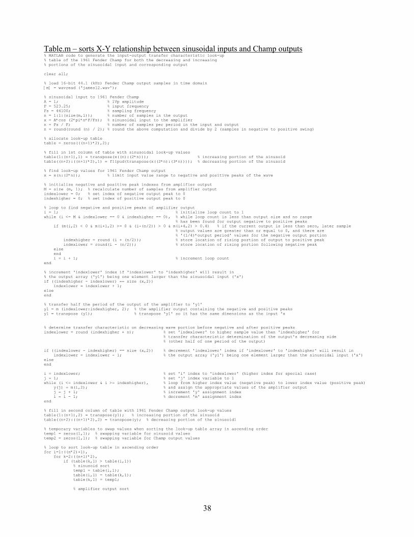
Table.m – sorts X-Y relationship between sinusoidal inputs and Champ outputs % MATLAB code to generate the input-output transfer characteristic look-up % table of the 1961 Fender Champ for both the decreasing and increasing % portions of the sinusoidal input and corresponding output clear all; % load 16-bit 44.1 (kHz) Fender Champ output samples in time domain [m] = wavread ('james12.wav'); % sinusoidal input to 1961 Fender Champ A = 1; % 1Vp amplitude F = 523.25; % input frequency Fs = 44100; % sampling frequency n = 1:1:(size(m,1)); % number of samples in the output x = A*cos (2*pi*n*F/Fs); % sinusoidal input to the amplifier n = Fs / F; % number of samples per period in the input and output n = round(round (n) / 2); % round the above computation and divide by 2 (samples in negative to positive swing) % allocate look-up table table = zeros(((n+1)*2),2); % fill in 1st column of table with sinusoidal look-up values table(1:(n+1),1) = transpose(x((n):(2*n))); % increasing portion of the sinusoid table((n+2):((n+1)*2),1) = flipud(transpose(x((2*n):(3*n)))); % decreasing portion of the sinusoid % find look-up values for 1961 Fender Champ output x = x(n:(2*n)); % limit input value range to negative and positive peaks of the wave % initialize negative and positive peak indexes from amplifier output M = size (m, 1); % recalculate number of samples from amplifier output indexlower = 0; % set index of negative output peak to 0 indexhigher = 0; % set index of positive output peak to 0 % loop to find negative and positive peaks of amplifier output i = 1; % initialize loop count to 1 while (i <= M & indexlower == 0 & indexhigher == 0), % while loop count is less than output size and no range % has been found for output negative to positive peaks if (m(i,2) < 0 & m(i+1,2) >= 0 & (i-(n/2)) > 0 & m(i+4,2) > 0.4) % if the current output is less than zero, later sample % output values are greater than or equal to 0, and there are % '(1/4)*output period' values for the negative output portion indexhigher = round (i + (n/2)); % store location of rising portion of output to positive peak indexlower = round(i - (n/2)); % store location of rising portion following negative peak else end i = i + 1; % increment loop count end % increment 'indexlower' index if 'indexlower' to 'indexhigher' will result in % the output array ('y1') being one element larger than the sinusoidal input ('x') if ((indexhigher - indexlower) == size (x,2)) indexlower = indexlower + 1; else end % transfer half the period of the output of the amplifier to 'y1' y1 = m (indexlower:indexhigher, 2); % the amplifier output containing the negative and positive peaks y1 = transpose (y1); % transpose 'y1' so it has the same dimensions as the input 'x % determine transfer characteristic on decreasing wave portion before negative and after positive peaks indexlower = round (indexhigher + n); % set 'indexlower' to higher sample value than 'indexhigher' for % transfer characteristic determination of the output's decreasing side % (other half of one period of the output) if ((indexlower - indexhigher) == size (x,2)) % decrement 'indexlower' index if 'indexlower' to 'indexhigher' will result in indexlower = indexlower - 1; % the output array ('y1') being one element larger than the sinusoidal input ('x') else end i = indexlower; % set 'i' index to 'indexlower' (higher index for special case) j = 1; % set 'j' index variable to 1 while (i <= indexlower & i >= indexhigher), % loop from higher index value (negative peak) to lower index value (positive peak) y(j) = m(i,2); % and assign the appropriate values of the amplifier output j = j + 1; % increment 'y' assignment index i = i - 1; % decrement 'm' assignment index end % fill in second column of table with 1961 Fender Champ output look-up values table(1:(n+1),2) = transpose(y1); % increasing portion of the sinusoid table((n+2):((n+1)*2),2) = transpose(y); % decreasing portion of the sinusoid1 % temporary variables to swap values when sorting the look-up table array in ascending order temp1 = zeros(1,1); % swapping variable for sinusoid values temp2 = zeros(1,1); % swapping variable for Champ output values % loop to sort look-up table in ascending order for i=1:((n*2)+1), for k=2:((n+1)*2), if (table(k,1) > table(i,1)) % sinusoid sort temp1 = table(i,1); table(i,1) = table(k,1); table(k,1) = temp1; % amplifier output sort

39

temp2 = table(i,2); table(i,2) = table(k,2); table(k,2) = temp2; else end end end % clear some variables clear temp1; clear temp2; clear x; clear y1; clear y; % plot input-output transfer characteristic figure (1), plot(table(:,1),table(:,2)), title ('1961 Fender Champ (Volume 12) Input-Output Transfer Characteristic for 1Vp 523.25 (Hz) Sinusoidal Input'), xlabel ('input x(n)'), ylabel ('output y(n)')

40

1961 Fender Champ Model Executable Code from Embedded Target for TI C6000TM DSP in MATLAB 6.5