Experiment No: - 01

Aim: To familiarize with MATLAB software, general functions and signal

processing toolbox functions.

The name MATLAB stands for MATrix LABoratory produced by Mathworks Inc.,

USA. It is a matrix-based powerful software package for scientific and engineering

computation and visualization. Complex numerical problems can be solved in a

fraction of the time that required with other high level languages. It provides an

interactive environment with hundreds of built -in –functions for technical

computation, graphics and animation. In addition to built-in-functions, user can create

his own functions.

MATLAB offers several optional toolboxes, such as signal processing, control

systems, neural networks etc.

It is command driven software and has online help facility.

MATLAB has three basic windows normally; command window, graphics window

and edit window.

Command window is characterized by the prompt ‘>>’.

All commands and the ready to run program filename can be typed here. Graphic

window gives the display of the figures as the result of the program. Edit window is to

create program files with an extension .m.

Some important commands in MATLAB Help List topics on which help is available

Help command name Provides help on the topic selected

Demo Runs the demo program

Who Lists variables currently in the workspace

Whos Lists variables currently in the workspace with their size

Clear Clears the workspace, all the variables are removed

Clear x,y,z Clears only variables x,y,z

Quit Quits MATLAB

Some of the frequently used built-in-functions in Signal Processing Toolbox filter(b.a.x) Syntax of this function is Y = filter(b.a.x)

It filters the data in vector x with the filter described by vectors

a and b to create the filtered data y.

fft (x) It is the DFT of vector x

ifft (x) It is the DFT of vector x

conv (a,b) Syntax of this function is C = conv (a,b) It convolves vectors a and b. The

resulting vector is of

Length, Length (a) + Length (b)-1

deconv(b,a) Syntax of this function is [q,r] = deconv(b,a)

It deconvolves vector q and the remainder in vector r such that

b = conv(a,q)+r

butter(N,Wn) designs an Nth order lowpass digital

Butterworth filter and returns the filter coefficients in length N+1 vectors B

(numerator) and A (denominator). The coefficients are listed in descending powers of

z. The cutoff frequency Wn must be 0.0 < Wn < 1.0, with 1.0 corresponding to half

the sample rate.

buttord(Wp, Ws, Rp, Rs) returns the order N of the lowest order digital Butterworth

filter that loses no more than Rp dB in the passband and has at least Rs dB of

attenuation in the stopband. Wp and Ws are the passband and stopband edge

frequencies, Normalized from 0 to 1 ,(where 1 corresponds to pi rad/sec)

Cheby1(N,R,Wn) designs an Nth order lowpass digital Chebyshev filter with R

decibels of peak-to-peak ripple in the passband. CHEBY1 returns the filter

coefficients in length N+1 vectors B (numerator) and A (denominator). The cutoff

frequency Wn must be 0.0 < Wn < 1.0, with 1.0 corresponding to half the sample rate.

Cheby1(N,R,Wn,'high') designs a highpass filter.

Cheb1ord(Wp, Ws, Rp, Rs) returns the order N of the lowest order digital Chebyshev

Type I filter that loses no more than Rp dB in the passband and has at least Rs dB of

attenuation in the stopband. Wp and Ws are the passband and stopband edge

frequencies, normalized from 0 to 1 (where 1 corresponds to pi radians/sample)

cheby2(N,R,Wn) designs an Nth order lowpass digital Chebyshev filter with the

stopband ripple R decibels down and stopband edge frequency Wn. CHEBY2 returns

the filter coefficients in length N+1 vectors B (numerator) and A . The cutoff

frequency Wn must be 0.0 < Wn < 1.0, with 1.0 corresponding to half the sample rate.

cheb2ord(Wp, Ws, Rp, Rs) returns the order N of the lowest order digital Chebyshev

Type II filter that loses no more than Rp dB in the passband and has at least Rs dB of

attenuation in the stopband. Wp and Ws are the passband and stopband edge

frequencies,

abs(x) It gives the absolute value of the elements of x. When x is complex, abs(x) is

the complex modulus (magnitude) of the elements of x. Angle (H) It returns the phase

angles of a matrix with complex elements in radians.

freqz(b,a,N) Syntax of this function is [h,w] = freqz(b,a,N) returns the Npoint

frequency vector w in radians and the N-point complex frequency response vector h

of the filter b/a.

stem(y) It plots the data sequence y as stems from the x axis terminated with circles

for the data value.

stem(x,y) It plots the data sequence y at the values specified in x.

ploy(x,y) It plots vector y versus vector x. If x or y is a matrix, then the vector is

plotted versus the rows or columns of the matrix, whichever line up.

title(‘text’) It adds text at the top of the current axis.

xlabel(‘text’) It adds text beside the x-axis on the current axis.

ylabel(‘text’) It adds text beside the y-axis on the current axis.

Experiment No: - 02

AIM: - TO write a MATLAB program to common continues time signals

PROCEDURE:-

-file

\ Figure window

ALGORITHM:-

MATLAB CODE:- clc;

clear all;

close all;

t=0:.001:1;

f=input('Enter the value of frequency');

a=input('Enter the value of amplitude');

subplot(3,3,1);

y=a*sin(2*pi*f*t);

plot(t,y,'r');

xlabel('time');

ylabel('amplitude');

title('sine wave')

grid on;

subplot(3,3,2);

z=a*cos(2*pi*f*t);

plot(t,z);

xlabel('time');

ylabel('amplitude');

title('cosine wave')

grid on;

subplot(3,3,3);

s=a*square(2*pi*f*t);

plot(t,s);

xlabel('time');

ylabel('amplitude');

title('square wave')

grid on;

subplot(3,3,4);

plot(t,t);

xlabel('time');

ylabel('amplitude');

title('ramp wave')

grid on;

subplot(3,3,5);

plot(t,a,'r');

xlabel('time');

ylabel('amplitude');

title('unit step wave')

grid on;

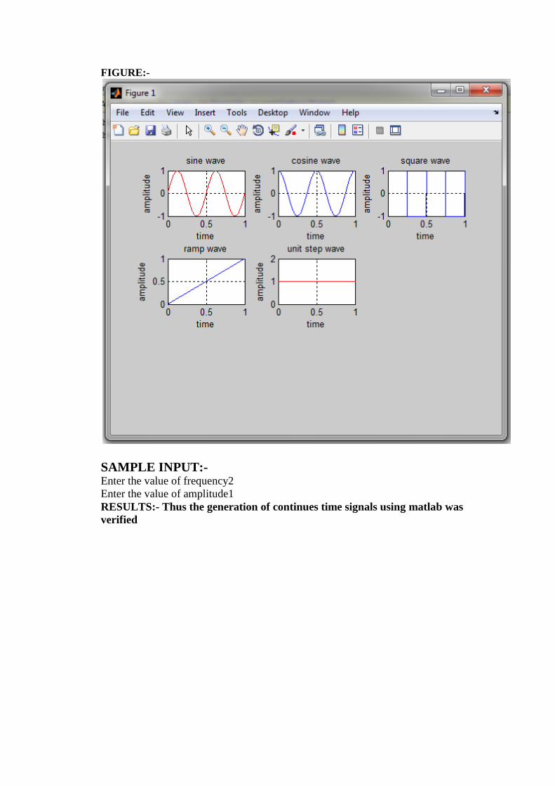
FIGURE:-

SAMPLE INPUT:- Enter the value of frequency2

Enter the value of amplitude1

RESULTS:- Thus the generation of continues time signals using matlab was

verified

Experiment No: - 03

AIM: - TO write a MATLAB program to common discrete time signals

PROCEDURE:-

-file

the output see command window\ Figure window

ALGORITHM:-

MATLAB CODE:- clc;

clear all;

close all;

n=0:1:50;

f=input('Enter the value of frequency');

a=input('Enter the value of amplitude');

N=input('Enter the length of unit step');

subplot(3,3,1);

y=a*sin(2*pi*f*n);

stem(n,y,'r');

xlabel('time');

ylabel('amplitude');

title('sine wave')

grid on;

subplot(3,3,2);

z=a*cos(2*pi*f*n);

stem(n,z);

xlabel('time');

ylabel('amplitude');

title('cosine wave')

grid on;

subplot(3,3,3);

s=a*square(2*pi*f*n);

stem(n,s);

xlabel('time');

ylabel('amplitude');

title('square wave')

grid on;

subplot(3,3,4);

stem(n,n);

xlabel('time');

ylabel('amplitude');

title('ramp wave')

grid on;

x=0:N-1;

d=ones(1,N);

subplot(3,3,5);

stem(x,d,'r');

xlabel('time');

ylabel('amplitude');

title('unit step wave')

grid on;

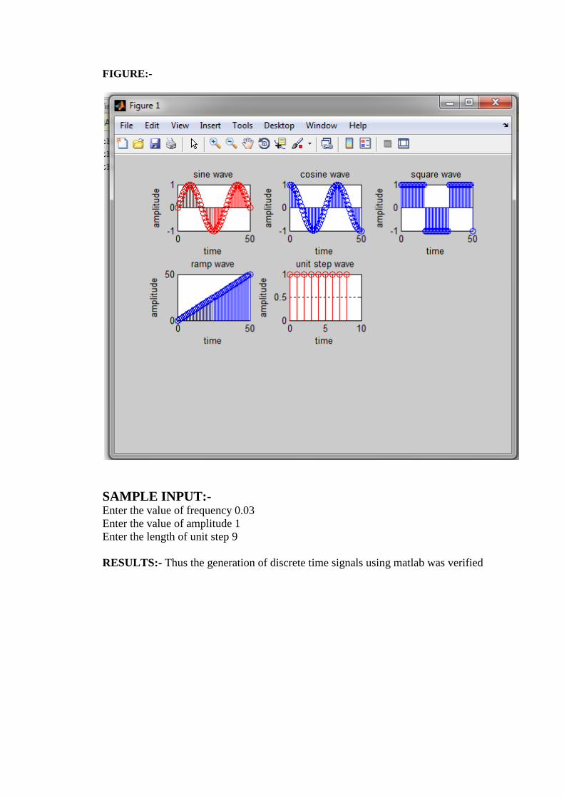
FIGURE:-

SAMPLE INPUT:- Enter the value of frequency 0.03

Enter the value of amplitude 1

Enter the length of unit step 9

RESULTS:- Thus the generation of discrete time signals using matlab was verified

Experiment No: - 04

AIM: - TO write a MATLAB program to compute linear convolution of two given

sequences

PROCEDURE:-

-file

the output see command window\ Figure window

ALGORITHM:-

MATLAB CODE:-

clc;

clear all;

close all;

a=input('Enter the starting point of x[n]=');

b=input('Enter the starting point of h[n]=');

x=input('Enter the co-efficients of x[n]=');

h=input('Enter the co-efficients of h[n]=');

y=conv(x,h);

subplot(3,1,1);

p=a:(a+length(x)-1);

stem(p,x);

grid on;

xlabel('Time');

ylabel('Amplitude');

title('INPUT x(n)');

subplot(3,1,2);

q=b:(b+length(h)-1);

stem(q,h);

grid on;

xlabel('Time');

ylabel('Amplitude');

title('IMPULSE RESPONSE h(n)');

subplot(3,1,3);

n=a+b:length(y)+a+b-1;

stem(n,y);

grid on;

disp(y)

xlabel('Time');

ylabel('Amplitude');

title('LINEAR CONVOLUTION');

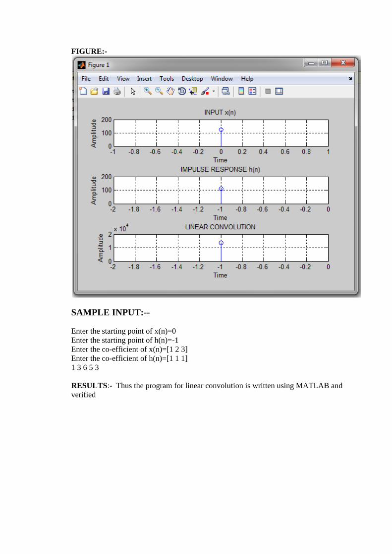
FIGURE:-

SAMPLE INPUT:--

Enter the starting point of x(n)=0

Enter the starting point of h(n)=-1

Enter the co-efficient of x(n)=[1 2 3]

Enter the co-efficient of h(n)=[1 1 1]

1 3 6 5 3

RESULTS:- Thus the program for linear convolution is written using MATLAB and

verified

Experiment No: - 05

AIM: - TO write a MATLAB program to compute circular convolution of two given

sequences

PROCEDURE:-

-file

\ Figure window

ALGORITHM:-

MATLAB CODE:-

clc;

clear;

a = input('enter the sequence x(n) = ');

b = input('enter the sequence h(n) = ');

n1=length(a);

n2=length(b);

N=max(n1,n2);

x = [a zeros(1,(N-n1))];

for i = 1:N

k = i;

for j = 1:n2

H(i,j)=x(k)* b(j);

k = k-1;

if (k == 0)

k = N;

end

end

end

y=zeros(1,N);

M=H';

for j = 1:N

for i = 1:n2

y(j)=M(i,j)+y(j);

end

end

disp('The output sequence is y(n)= ');

disp(y);

stem(y);

title('Circular Convolution');

xlabel('n');

ylabel('y(n)');

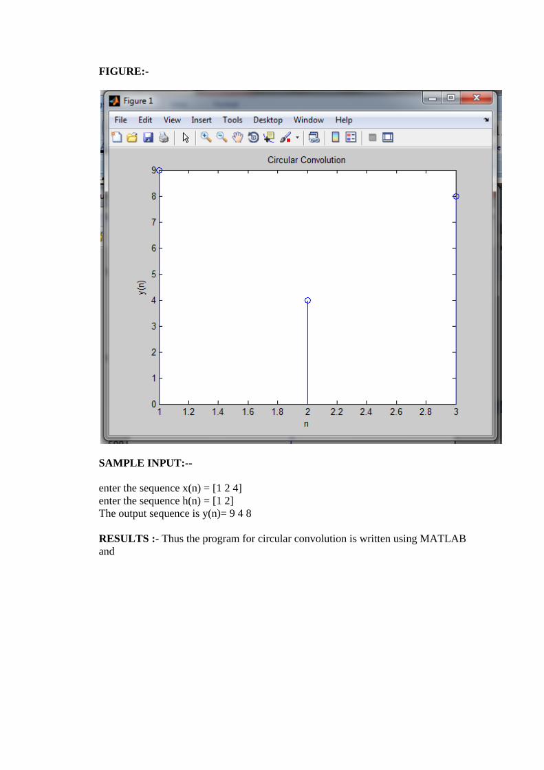
FIGURE:-

SAMPLE INPUT:--

enter the sequence x(n) = [1 2 4]

enter the sequence h(n) = [1 2]

The output sequence is y(n)= 9 4 8

RESULTS :- Thus the program for circular convolution is written using MATLAB

and

Experiment No: - 06

AIM: - TO write a MATLAB program to plot magnitude response and phase

response of digital

Butter worth Low pass filter

PROCEDURE:-

-file

ompile and Run the program

\ Figure window

ALGORITHM:-

MATLAB CODE:-

clc;

clear all;

close all;

rp=input('enter the passband attenuation:');

rs=input('enter the stop band attenuation:');

wp=input('enter the pass band frequency:');

ws=input('enter the stop band frequency:');

[N,wn]=buttord(wp/pi,ws/pi,rp,rs);

[b,a]=butter(N,wn);

freqz(b,a); YAMUNA INSTITUTE ENGINEERING & TECHNOLOGY DSP Lab manual using MATLAB Prepared By :-Ashwini Kumar

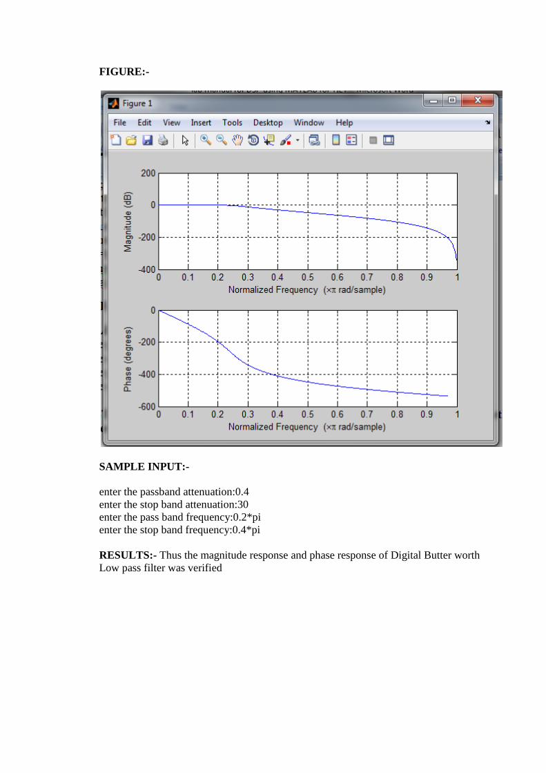
FIGURE:-

SAMPLE INPUT:-

enter the passband attenuation:0.4

enter the stop band attenuation:30

enter the pass band frequency:0.2*pi

enter the stop band frequency:0.4*pi

RESULTS:- Thus the magnitude response and phase response of Digital Butter worth

Low pass filter was verified

Experiment No: - 07 AIM: - TO write a MATLAB program to plot magnitude response and phase

response of digital Butter worth High pass filter

PROCEDURE:-

-file

ectory

\ Figure window

ALGORITHM:-

ion

MATLAB CODE:-

clc;

clear all;

close all;

rp=input ('Enter the pass band attenuation:');

rs=input ('Enter the stop band attenuation:');

wp=input ('Enter the pass band frequency:');

ws=input ('Enter the stop band frequency:');

[N,wn]=buttord(wp/pi,ws/pi,rp,rs);

[b,a]=butter(N,wn,'high');

freqz(b,a);

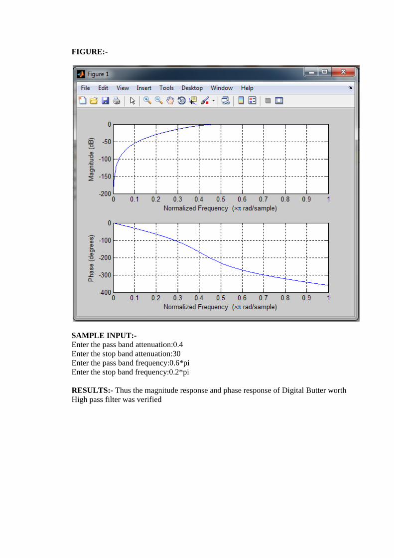
FIGURE:-

SAMPLE INPUT:- Enter the pass band attenuation:0.4

Enter the stop band attenuation:30

Enter the pass band frequency:0.6*pi

Enter the stop band frequency:0.2*pi

RESULTS:- Thus the magnitude response and phase response of Digital Butter worth

High pass filter was verified

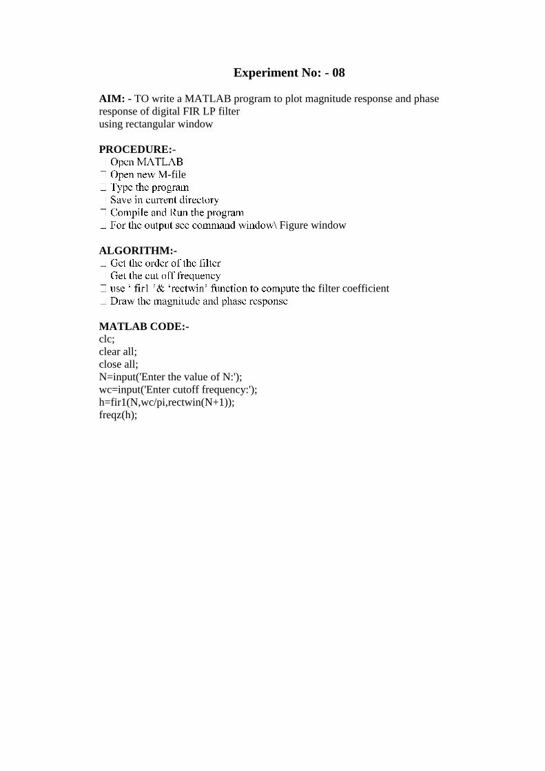
Experiment No: - 08

AIM: - TO write a MATLAB program to plot magnitude response and phase

response of digital FIR LP filter

using rectangular window

PROCEDURE:-

-file

\ Figure window

ALGORITHM:-

filter coefficient

MATLAB CODE:- clc;

clear all;

close all;

N=input('Enter the value of N:');

wc=input('Enter cutoff frequency:');

h=fir1(N,wc/pi,rectwin(N+1));

freqz(h);

FIGURE:-

SAMPLE INPUT:- Enter the value of N:28

Enter cutoff frequency:0.5*pi

RESULTS:- Thus the magnitude response and phase response of fir Low pass filter

using rectangular window was verified.

Experiment No: - 09

AIM: - TO write a MATLAB program to plot magnitude response and phase

response of digital FIR HP filter using rectangular window

PROCEDURE:-

-file

For the output see command window\ Figure window

ALGORITHM:-

MATLAB CODE:-

clc;

clear all;

close all;

N=input('Enter the value of N:');

wc=input('Enter cutoff frequency:');

h=fir1(N,wc/pi,'high',rectwin(N+1));

freqz(h);

FIGURE:-

SAMPLE INPUT:-

Enter the value of N:28

Enter cutoff frequency:0.5*pi

RESULTS:- Thus the magnitude response and phase response of fir High pass filter

using rectangular window was verified

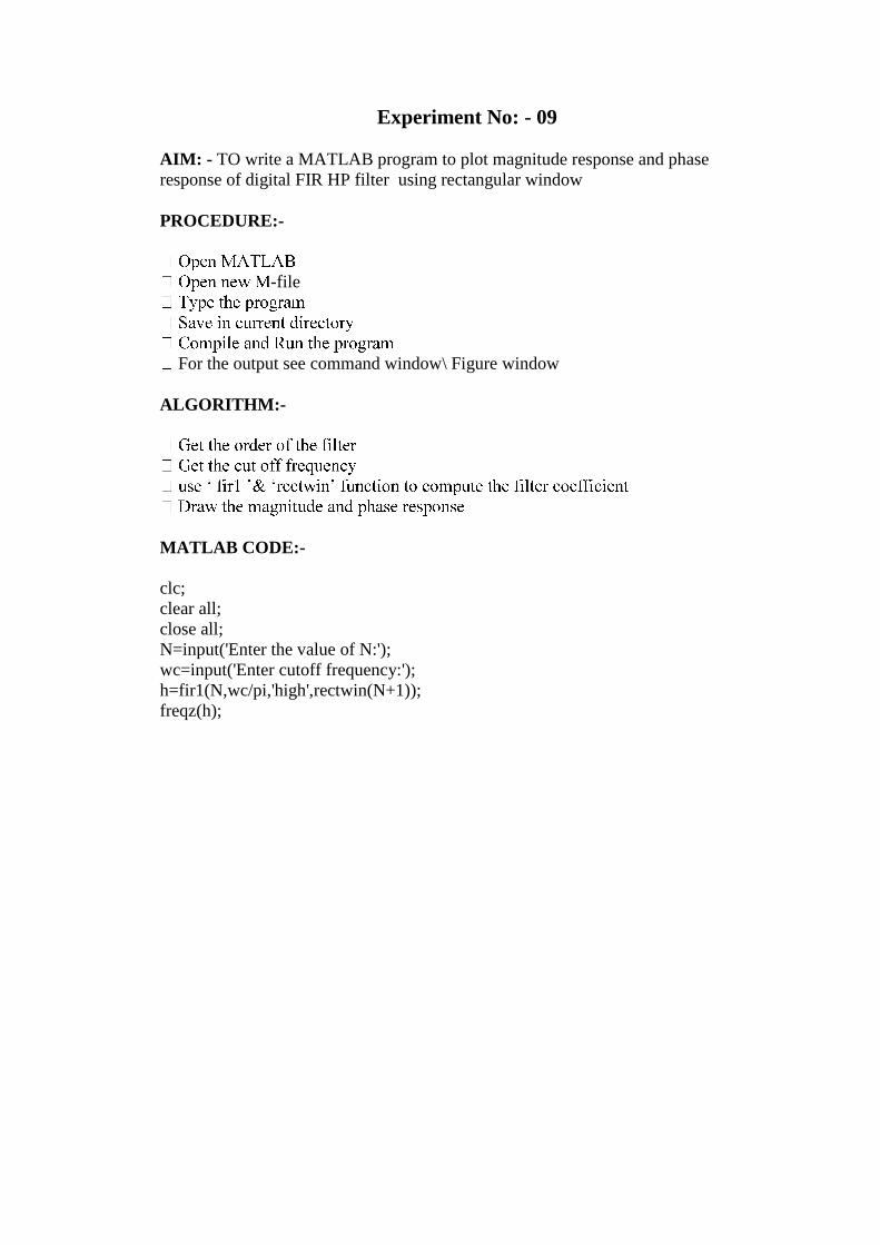
Experiment No: - 10

AIM: - TO write a MATLAB program to find the DFT of a sequence.

PROCEDURE:-

-file

\ Figure window

ALGORITHM:-

MATLAB CODE:-

clc;

clear all;

close all;

N=input('Enter the value of N');

x=input('Enter the input sequence X(n):');

t=0:N-1;

subplot(2,1,1);

stem(t,x);

xlabel('TIME');

ylabel('AMPLITUDE');

title('INPUT SIGNAL');

grid on;

y=fft(x,N)

subplot(2,1,2);

stem(t,y);

xlabel('TIME');

ylabel('AMPLITUDE');

title('OUTPUT SIGNAL');

grid on;

FIGURE:-

SAMPLE INPUT:-

Enter the value of N 4

Enter the input sequence X(n):[1 2 3 4]

y =

10.0000 + 0.0000i -2.0000 + 2.0000i -2.0000 + 0.0000i -2.0000 - 2.0000i

RESULTS:- Thus the program for dft is written using MATLAB and verified.

Experiment No: - 11

AIM: - TO write a MATLAB program to find the IDFT of a sequence

PROCEDURE:-

MATLAB

-file

\ Figure window

ALGORITHM:-

matlab function ‘ifft’

MATLAB CODE:-

clc;

clear all;

close all;

N=input('Enter the value of N=');

y=input('Enter the sequence y[n]=');

t=0:N-1;

subplot(2,1,1);

stem(t,y);

xlabel('TIME');

ylabel('AMPLITUDE');

title('INPUT SIGNAL');

grid on;

x=ifft(y,N)

subplot(2,1,2);

stem(t,x);

xlabel('TIME');

ylabel('AMPLITUDE');

title('OUTPUT SIGNAL');

grid on;

FIGURE:-

SAMPLE INPUT:-

Enter the value of N=4

Enter the sequence y[n]=[ 10.0000 + 0.0000i -2.0000 + 2.0000i -2.0000 + 0.0000i -

2.0000 - 2.0000i]

x =

1 2 3 4

RESULTS:- Thus the program for idft is written using MATLAB and verified.

Experiment No: - 12 AIM: - TO write a MATLAB program to plot magnitude response and phase

response of IIR Butter worth High pass filter

PROCEDURE:-

-file

see command window\ Figure window

Matlab code:-

clear all;

close all;

fp=input('Enter the pass band frequency fp = ');

fs=input('Enter the stop band frequency fs = ');

rp=input('Enter the pass band attenuation rp = ');

rs=input('Enter the stop band attenuation rs = ');

f=input ('Enter the sampling frequency f = ');

wp=2*fp/f;

ws=2*fs/f;

[n,wn]=buttord(wp,ws,rp,rs);

[b,a]=butter(n,wn,'low');

freqz(b,a,500,f);

title ('Magnitude and phase respose of the IIR butterworth filter');

FIGURE:-

SAMPLE INPUT:-

Enter the pass band frequency fp = 1000 Enter the stop band frequency fs = 1200

Enter the pass band attenuation rp = .2 Enter the stop band attenuation rs = 45 Enter

the sampling frequency f = 3000

RESULTS:- Thus the magnitude response and phase response of IIR Butter worth

filter was verified