28
DSS Performance in Oracle Database 11g An Oracle White Paper August 2007
DSS Performance in Oracle Database 11g
An Oracle White Paper
August 2007
DSS Performance in Oracle Database 11g Page 2
DSS Performance in Oracle Database 11g
Executive Overview.......................................................................................... 3 Introduction ....................................................................................................... 3 Test Environment ............................................................................................. 4 Result Cache....................................................................................................... 7 What to expect from Result Cache in your application? ........................ 9
OCI Client Result Cache.................................................................................. 9 Composite Partitioning................................................................................... 12 Full Outer Join................................................................................................. 15 Min and Max Aggregation ............................................................................. 18 Nested Loop Join ............................................................................................ 19 DBMS_STATS Package Improvements – NDV....................................... 21 Incremental Maintenance of NDV for Partitioned Table......................... 24 Conclusion........................................................................................................ 27
DSS Performance in Oracle Database 11g Page 3
DSS Performance in Oracle database 11g
EXECUTIVE OVERVIEW
This technical white paper introduces new performance features and
enhancements in Oracle Database 11g for data warehouses and decision support
systems. The performance gains of Oracle Database 11g over Oracle Database 10g
Release 2 are demonstrated via detailed query examples. Performance results show
that upgrading to Oracle Database 11g can significantly improve performance and
scalability of DSS applications.
INTRODUCTION
For many successful enterprises, data warehouse applications drive business
initiatives and generate revenue opportunities. Data warehouse and decision
support systems (DSS) have become so mission critical that system performance
directly impacts the bottom line.
However, according to the latest Winter Corp Top Ten Program1, the size of the
world’s largest databases has tripled every two years since 2001. The fast growth of
database sizes can result in slower system performance, negatively impacting the
system’s ability to provide superior service and support. Even though hardware
processor performance advances rather rapidly as Moore’s law has predicted, it is
not enough to meet the performance challenge because the size of databases grows
even faster than processor speed. This drives the demands for further software
innovations to improve the overall system performances of DSS applications.
Oracle Database 11g is designed to address the challenge, delivering a high
performance system to meet today’s fast growing data warehousing requirement. It
contains new features and enhancements that improve overall system
performance. Upgrading to Oracle Database 11g can significantly improve system
performance and scalability.
This technical white paper describes these new features and enhancements.
Concrete query examples are provided to compare the performance in Oracle
Database 10g Release 2 and Oracle Database 11g. In the subsequent sections, the
test environment is described first, followed by the descriptions of the new
features and enhancements and the performance tests.
1 http://www.wintercorp.com/VLDB/2005_TopTen_Survey/TopTenProgram.html
DSS Performance in Oracle Database 11g Page 4
TEST ENVIRONMENT
Tests in this white paper were conducted on a system with 2x2.8 GHz Intel Xeon
processors with Hyper-Threading technology simulating 4 CPUs. The system has 7
GB of memory. The operating system is Oracle Enterprise Linux 4. The databases
were created on an ASM disk group built with10 disks in a single disk array (EMC
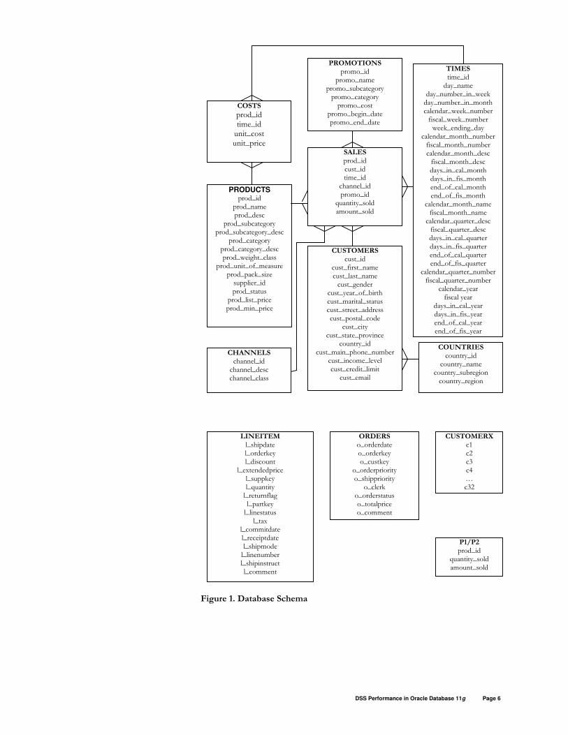
Clariion CX300). The database schema, portrayed by Figure 1, consists of the
Sales History schema from Oracle Sample Schema, part of the TPC-H schema,
and a few other independent tables.
The Sales History schema in Oracle Sample Schema tracks business statistics to
facilitate business decisions. The SALES table is populated with 10 years worth of
sales information, from Jan 1995 to Dec 2004, totaling about 10 GB of data. Both
the SALES table and COSTS table are compressed and are range-partitioned on
time_id, and the total number of partitions is 32.
TPC-H is widely accepted as the industry standard benchmark for data
warehousing applications. Its schema consists of eight tables modeling the data
warehouse of a typical retail environment. Among the eight tables, we use the
largest two tables, the LINEITEM and ORDERS tables. These two tables are
generated via the standard TPC-H data generator “dbgen” with scale factor set to
30. Both tables contain 84 partitions and each partition contains 8 sub-partitions.
The LINEITEM table is range-partitioned by l_shipdate at top level and hash
partitioned by l_partkey at sub-partition level. The ORDERS table is range-
partitioned by o_orderdate at top level and hash partitioned by o_custkey at sub-
partition level.
CUSTOMERX table is real-world customer data extracted from the data
warehouse belonging to one of the largest financial organizations. It contains
records of business transactions. This data set is highly skewed, reflecting real-
world business data distribution. It has 32 columns and 213 million rows in 10
partitions. The last partition is empty. The total size of this data set is 34 GB.
Table P1 and P2 are synthetically generated tables containing “quantity sold” and
“amount sold” information for different products. Table P1 contains information
from period 1, and table P2 contains information from period 2.
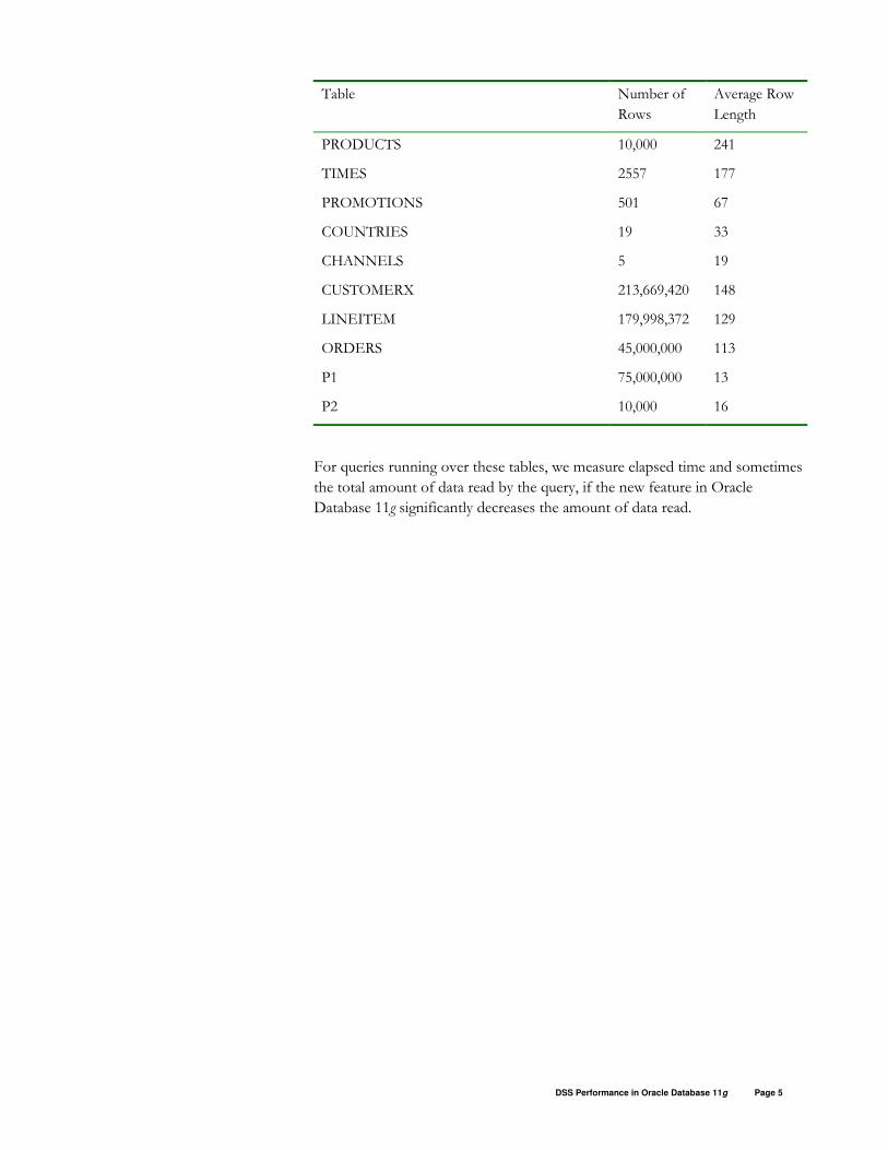
The table below lists the number-of-rows and average-row-length statistics for
each table.
Table Number of
Rows
Average Row
Length
SALES 300,000,000 31
COSTS 14,600,000 20
CUSTOMERS 50,000 138
DSS Performance in Oracle Database 11g Page 5
Table Number of
Rows
Average Row
Length
PRODUCTS 10,000 241
TIMES 2557 177
PROMOTIONS 501 67
COUNTRIES 19 33
CHANNELS 5 19
CUSTOMERX 213,669,420 148
LINEITEM 179,998,372 129
ORDERS 45,000,000 113
P1 75,000,000 13
P2 10,000 16
For queries running over these tables, we measure elapsed time and sometimes
the total amount of data read by the query, if the new feature in Oracle
Database 11g significantly decreases the amount of data read.
DSS Performance in Oracle Database 11g Page 6
Figure 1. Database Schema
COSTS
prod_id time_id unit_cost unit_price
PRODUCTS prod_id
prod_name prod_desc
prod_subcategory prod_subcategory_desc
prod_category prod_category_desc prod_weight_class
prod_unit_of_measure prod_pack_size supplier_id prod_status
prod_list_price prod_min_price
PROMOTIONS promo_id
promo_name promo_subcategory promo_category promo_cost
promo_begin_date promo_end_date
SALES prod_id cust_id time_id
channel_id promo_id
quantity_sold amount_sold
CHANNELS channel_id channel_desc channel_class
CUSTOMERS cust_id
cust_first_name cust_last_name cust_gender
cust_year_of_birth cust_marital_status cust_street_address cust_postal_code
cust_city cust_state_province
country_id cust_main_phone_number
cust_income_level cust_credit_limit cust_email
TIMES time_id day_name
day_number_in_week day_number_in_month calendar_week_number fiscal_week_number week_ending_day
calendar_month_number fiscal_month_number calendar_month_desc fiscal_month_desc days_in_cal_month days_in_fis_month end_of_cal_month end_of_fis_month
calendar_month_name fiscal_month_name calendar_quarter_desc fiscal_quarter_desc days_in_cal_quarter days_in_fis_quarter end_of_cal_quarter end_of_fis_quarter
calendar_quarter_number fiscal_quarter_number
calendar_year fiscal year
days_in_cal_year days_in_fis_year end_of_cal_year end_of_fis_year
COUNTRIES country_id
country_name country_subregion country_region
ORDERS o_orderdate o_orderkey o_custkey
o_orderpriority o_shippriority
o_clerk o_orderstatus o_totalprice o_comment
LINEITEM l_shipdate l_orderkey l_discount
l_extendedprice l_suppkey l_quantity l_returnflag l_partkey l_linestatus l_tax
l_commitdate l_receiptdate l_shipmode l_linenumber l_shipinstruct l_comment
CUSTOMERX c1 c2 c3 c4 … c32
P1/P2 prod_id
quantity_sold amount_sold
DSS Performance in Oracle Database 11g Page 7
RESULT CACHE
To speed up query execution for systems with large memories, Oracle Database
11g provides a mechanism to cache results of queries and query fragments in
memory. The cached results reside in the Result Cache memory allocated from the
SGA; it will be used to answer future executions of these queries and query
fragments. Since results of query fragments can be cached, different queries that
have common sub-execution plans can share cached results.
When cached results are used, Oracle Database 11g answers the query or query
fragments immediately regardless of how long it takes to actually execute the query
or query fragments. A traditionally long-running query that retrieves only a small
result set can see a near infinite performance improvement if the result is served
out of the cache. A subsequent execution of the same query or query fragment is
required in order to take advantage of the cached result.
The lifetime of any cached result is independent of the cursor that created it;
however, to ensure correctness, cached results will be automatically invalidated
when any of the database objects used in its creation are successfully modified.
DSS applications mostly access read-only and read-mostly data; data modification
happens infrequently, making them ideal candidates to take advantage of Result
Cache.
There are different ways to enable Oracle Database 11g to cache results of queries
or query fragments. The easiest way is to annotate the query or query fragment
with a “result_cache” hint. For example, query Q1 below returns the costs and
revenues associated with each promotion. It contains a sub query which returns
revenues associated with each promotion id. Both query Q1 and the sub-query are
annotated with the “result_cache” hint.
Q1:
select /*+ result_cache */ p.promo_name promotion,
p.promo_cost cost,
s.revenue revenue
from promotions p,
( select /*+ result_cache */
promo_id promo_id, sum(amount_sold) revenue
from sales
group by promo_id ) s
where s.promo_id = p.promo_id
order by s.revenue desc;
These two “result_cache” hints indicate the query blocks in both SELECT
statements are to have their results cached. During query execution, Result Cache
is interrogated to see if a result for the underlying execution plan already exists in
the Result Cache. If the result is found in the Result Cache, then the execution of
the underlying execution plan is bypassed; otherwise the Oracle server will execute
the query and return the result as output, but as a side-effect the result is also
stored in the Result Cache.

DSS Performance in Oracle Database 11g Page 8
To demonstrate the dramatic query performance improvement by sharing results
stored in the Result Cache, we consider the following queries as well:
Q2:
select /*+ result_cache */
promo_id promo_id, sum(amount_sold) revenue
from sales
group by promo_id;
This is the sub query in Q1. It is hinted with the “result_cache” hint so that the
Result Cache will be interrogated when this query is run. In our running example,
we run the query separately after query Q1 is run to demonstrate the ability of
query Q2 sharing results in Result Cache created by query Q1.
The following query Q3 is also run after query Q1 to show that results for query
fragments can be shared among different queries.
Q3:
select p.promo_name promotion,
s.revenue revenue
from promotions p,
( select /*+ result_cache */
promo_id promo_id, sum(amount_sold) revenue
from sales
group by promo_id ) s
where s.promo_id = p.promo_id
order by s.revenue desc;
Query Q3 has the same sub query as Q1, but it selects only promotion and
revenue, instead of promotion, costs, and revenue selected in query Q1. The sub
query in Q3 is also hinted with the “result_cache” hint to allow it to create result
cache entries or get results from the Result Cache.
To compare with Oracle Database 10g Release 2, we run the above queries in the
following sequence after database startup in both Oracle Database 11g and Oracle
Database 10g Release 2:
Q1, Q1, Q2, Q3
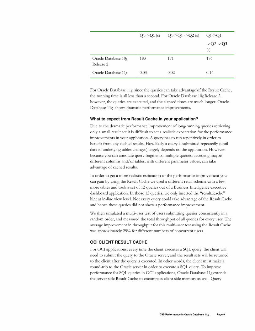
We measure the elapsed time of the second run of Q1, and the elapsed time of Q2,
and Q3. The following table summarizes the results. The column headings show
what we have run so far, for example, Q1->Q1 means that we ran Q1, and then
run Q1 again. The highlighted query name is the one that is measured and the
elapsed time results are shown in that column. For example, Q1->Q1 means that
what are shown in that column are the elapsed time results of the second run of
query Q1.
DSS Performance in Oracle Database 11g Page 9
Q1->Q1 (s) Q1->Q1 ->Q2 (s) Q1->Q1
->Q2 ->Q3
(s)
Oracle Database 10g
Release 2
183 171 176
Oracle Database 11g 0.03 0.02 0.14
For Oracle Database 11g, since the queries can take advantage of the Result Cache,
the running time is all less than a second. For Oracle Database 10g Release 2,
however, the queries are executed, and the elapsed times are much longer. Oracle
Database 11g shows dramatic performance improvements.
What to expect from Result Cache in your application?
Due to the dramatic performance improvement of long-running queries retrieving
only a small result set it is difficult to set a realistic expectation for the performance
improvements in your application. A query has to run repetitively in order to
benefit from any cached results. How likely a query is submitted repeatedly (until
data in underlying tables changes) largely depends on the application. However
because you can annotate query fragments, multiple queries, accessing maybe
different columns and/or tables, with different parameter values, can take
advantage of cached results.
In order to get a more realistic estimation of the performance improvement you
can gain by using the Result Cache we used a different retail schema with a few
more tables and took a set of 12 queries out of a Business Intelligence executive
dashboard application. In those 12 queries, we only inserted the “result_cache”
hint at in-line view level. Not every query could take advantage of the Result Cache
and hence these queries did not show a performance improvement.
We then simulated a multi-user test of users submitting queries concurrently in a
random order, and measured the total throughput of all queries for every user. The
average improvement in throughput for this multi-user test using the Result Cache
was approximately 25% for different numbers of concurrent users.
OCI CLIENT RESULT CACHE
For OCI applications, every time the client executes a SQL query, the client will
need to submit the query to the Oracle server, and the result sets will be returned
to the client after the query is executed. In other words, the client must make a
round-trip to the Oracle server in order to execute a SQL query. To improve
performance for SQL queries in OCI applications, Oracle Database 11g extends
the server side Result Cache to encompass client side memory as well. Query
DSS Performance in Oracle Database 11g Page 10
results can be cached at the client side so that subsequent query executions in OCI
applications can access the locally cached result sets without fetching rows from
the server.
The client-side result cache is per process so that multiple client sessions can
simultaneously use matching cached result sets. Each combination of SQL text and
bind values will have their own cached result sets. Any application that uses OCI
to connect to the database can take advantage of the cache. The client-side result
cache can work with or without server-side result cache. The cached result set data
at the client-side is transparently kept consistent with any changes done on the
server side.
By leveraging additional cheaper client-side memory to eliminate the network
round trip to the server, OCI client result cache can significantly improve
performances for client SQL query executions and row fetching. By having cache
on the clients, we can also get good locality of reference to client applications.
Repeatedly executed queries in client applications will be resolved at the client
caches and will not be present in the stream of requests passed on to the server.
Since the server sees only those queries that miss at the clients, the scalability of
Oracle server will also be increased.
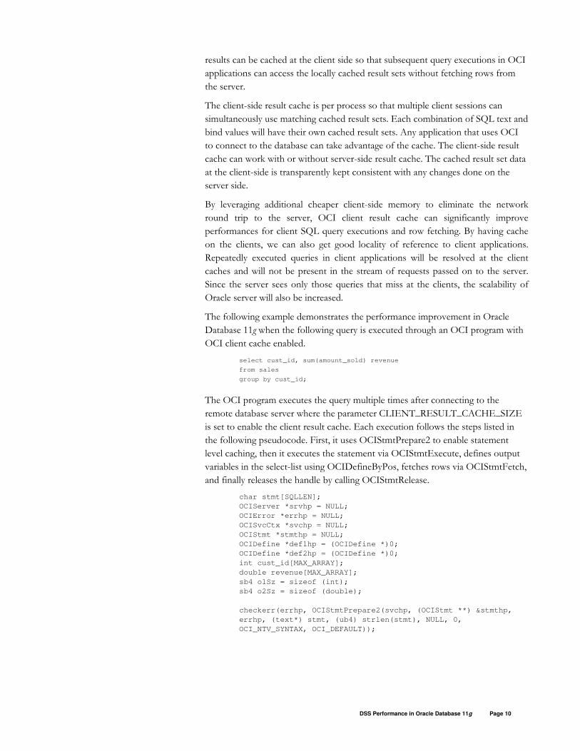
The following example demonstrates the performance improvement in Oracle
Database 11g when the following query is executed through an OCI program with
OCI client cache enabled.
select cust_id, sum(amount_sold) revenue
from sales
group by cust_id;
The OCI program executes the query multiple times after connecting to the
remote database server where the parameter CLIENT_RESULT_CACHE_SIZE
is set to enable the client result cache. Each execution follows the steps listed in
the following pseudocode. First, it uses OCIStmtPrepare2 to enable statement
level caching, then it executes the statement via OCIStmtExecute, defines output
variables in the select-list using OCIDefineByPos, fetches rows via OCIStmtFetch,
and finally releases the handle by calling OCIStmtRelease.
char stmt[SQLLEN];
OCIServer *srvhp = NULL;
OCIError *errhp = NULL;
OCISvcCtx *svchp = NULL;
OCIStmt *stmthp = NULL;
OCIDefine *def1hp = (OCIDefine *)0;
OCIDefine *def2hp = (OCIDefine *)0;
int cust_id[MAX_ARRAY];
double revenue[MAX_ARRAY];
sb4 o1Sz = sizeof (int);
sb4 o2Sz = sizeof (double);
checkerr(errhp, OCIStmtPrepare2(svchp, (OCIStmt **) &stmthp,
errhp, (text*) stmt, (ub4) strlen(stmt), NULL, 0,
OCI_NTV_SYNTAX, OCI_DEFAULT));

DSS Performance in Oracle Database 11g Page 11
checkerr(errhp, OCIStmtExecute(svchp, stmthp, errhp, 0, 0,
NULL, NULL, OCI_RESULT_CACHE));
checkerr(errhp, OCIDefineByPos(stmthp, (OCIDefine **)&def1hp,
errhp, (ub4)1, (int *)cust_id, o1Sz, (ub2)OCI_TYPECODE_INTEGER,
(dvoid *)0, (ub2 *)0, (ub2 *)0, (ub4)OCI_DEFAULT));
checkerr(errhp, OCIDefineByPos(stmthp, (OCIDefine **)&def2hp,
errhp, (ub4)2, (double *)revenue, o2Sz,
(ub2)OCI_TYPECODE_FLOAT, (dvoid *)0, (ub2 *)0, (ub2 *)0,
(ub4)OCI_DEFAULT));
while ((status =OCIStmtFetch(stmthp, errhp, MAX_ARRAY,
(ub2)OCI_FETCH_NEXT, (ub4)OCI_DEFAULT)) == OCI_SUCCESS) {
/* print fetched rows in cust_id[i] and revenue[i] */
}
OCIStmtRelease(stmthp, errhp, NULL, 0, OCI_DEFAULT);
Our OCI client is in Austin, TX, while the database server is in Redwood Shores,
CA. For Oracle Database 11g, query results are cached at the client side after the
very first run, and subsequent runs of the same query are resolved at the client-side
cache. The number of rows fetched from the server to client is 50,000. The set up
for Oracle Database 10g Release 2 is the same except that no client result cache is
used. For both Oracle Database 11g and Oracle Database 10g Release 2, we
measure the performance of the second run of the query. The time measured is the
time spent between OCIStmtRrepare2 call and OCIStmtRelease call in the above
pseudocode. The table below lists the performance results.
Elapsed Time (s)
Oracle Database 10g Release 2 265
Oracle Database 11g 0.27
As we can see from the above table, with client side result cache, the second run of
the query in Oracle Database 11g only takes 0.27 seconds because data can be
retrieved directly from local cache. In Oracle Database 10g Release 2, however, the
query needs to be submitted to the Oracle server for execution. Query results are
fetched from server to client. It takes 265 seconds. For this example Oracle
Database 11g is three orders of magnitude faster than Oracle Database 10g Release
2.
With OCI client result cache, Oracle Database 11g not only gets results for user in
a fraction of a second in this case, but also dramatically decreases the load on
server, allowing the server to accommodate more concurrent requests from other
users and/or applications.
This dramatic performance improvement is demonstrated by a test case that
executes the same query multiple times over a read-only table. For a more complex
client applications where multiple queries are submitted and updates may occur,
DSS Performance in Oracle Database 11g Page 12
the performance improvement because of the OCI client result cache feature will
depend on a few factors, such as how often queries are repeated, how often
updates occur, and the client result cache size.
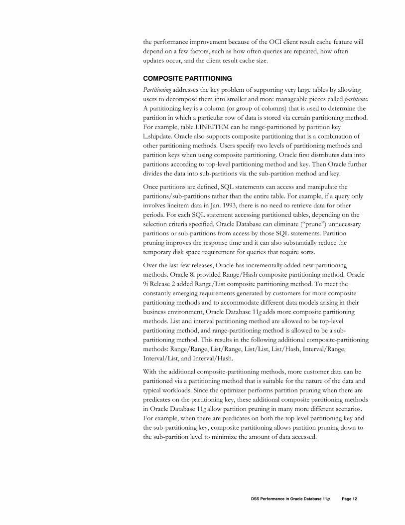
COMPOSITE PARTITIONING
Partitioning addresses the key problem of supporting very large tables by allowing
users to decompose them into smaller and more manageable pieces called partitions.
A partitioning key is a column (or group of columns) that is used to determine the
partition in which a particular row of data is stored via certain partitioning method.
For example, table LINEITEM can be range-partitioned by partition key
l_shipdate. Oracle also supports composite partitioning that is a combination of
other partitioning methods. Users specify two levels of partitioning methods and
partition keys when using composite partitioning. Oracle first distributes data into
partitions according to top-level partitioning method and key. Then Oracle further
divides the data into sub-partitions via the sub-partition method and key.
Once partitions are defined, SQL statements can access and manipulate the
partitions/sub-partitions rather than the entire table. For example, if a query only
involves lineitem data in Jan. 1993, there is no need to retrieve data for other
periods. For each SQL statement accessing partitioned tables, depending on the
selection criteria specified, Oracle Database can eliminate (“prune”) unnecessary
partitions or sub-partitions from access by those SQL statements. Partition
pruning improves the response time and it can also substantially reduce the
temporary disk space requirement for queries that require sorts.
Over the last few releases, Oracle has incrementally added new partitioning
methods. Oracle 8i provided Range/Hash composite partitioning method. Oracle
9i Release 2 added Range/List composite partitioning method. To meet the
constantly emerging requirements generated by customers for more composite
partitioning methods and to accommodate different data models arising in their
business environment, Oracle Database 11g adds more composite partitioning
methods. List and interval partitioning method are allowed to be top-level
partitioning method, and range-partitioning method is allowed to be a sub-
partitioning method. This results in the following additional composite-partitioning
methods: Range/Range, List/Range, List/List, List/Hash, Interval/Range,
Interval/List, and Interval/Hash.
With the additional composite-partitioning methods, more customer data can be
partitioned via a partitioning method that is suitable for the nature of the data and
typical workloads. Since the optimizer performs partition pruning when there are
predicates on the partitioning key, these additional composite partitioning methods
in Oracle Database 11g allow partition pruning in many more different scenarios.
For example, when there are predicates on both the top level partitioning key and
the sub-partitioning key, composite partitioning allows partition pruning down to
the sub-partition level to minimize the amount of data accessed.

DSS Performance in Oracle Database 11g Page 13
To demonstrate the benefits of the additional composite-partitioning methods, we
compare the Range/Range composite-partitioning method in Oracle Database 11g
with the Range-partitioning method in Oracle Database 10g Release 2. We
consider the LINEITEM table in TPC-H schema. In Oracle Database 10g Release
2, the LINEITEM table is range-partitioned using l_shipdate as partitioning key.
There are 84 total partitions.
create table lineitem(
l_shipdate date NOT NULL,
l_orderkey number NOT NULL,
l_discount number NOT NULL,
l_extendedprice number NOT NULL,
l_suppkey number NOT NULL,
l_quantity number NOT NULL,
l_returnflag char(1) NOT NULL,
l_partkey number NOT NULL,
l_linestatus char(1) NOT NULL,
l_tax number NOT NULL,
l_commitdate date NOT NULL,
l_receiptdate date NOT NULL,
l_shipmode char(10) NOT NULL,
l_linenumber number NOT NULL,
l_shipinstruct char(25) NOT NULL,
l_comment varchar(44)
)
pctfree 1 pctused 99 initrans 10 storage (freelists 99)
parallel nologging
partition by range (l_shipdate)
(
partition item1 values less than (to_date('1992-01-01','YYYY-MM-DD')),
partition item2 values less than (to_date('1992-02-01','YYYY-MM-DD')),
……
partition item82 values less than (to_date('1998-10-01','YYYY-MM-DD')),
partition item83 values less than (to_date('1998-11-01','YYYY-MM-DD')),
partition item84 values less than (MAXVALUE));
In Oracle Database 11g, we use Range/Range partitioning method to partition the
LINEITEM table via l_shipdate at the top level and l_commitdate at the sub-
partitioning level:
create table lineitem(
l_shipdate date NOT NULL,
l_orderkey number NOT NULL,
l_discount number NOT NULL,
l_extendedprice number NOT NULL,
l_suppkey number NOT NULL,
l_quantity number NOT NULL,
l_returnflag char(1) NOT NULL,
l_partkey number NOT NULL,
l_linestatus char(1) NOT NULL,
l_tax number NOT NULL,
l_commitdate date NOT NULL,
l_receiptdate date NOT NULL,
l_shipmode char(10) NOT NULL,
l_linenumber number NOT NULL,
l_shipinstruct char(25) NOT NULL,
l_comment varchar(44)
)
pctfree 1 pctused 99 initrans 10 storage (freelists 99)
parallel nologging
DSS Performance in Oracle Database 11g Page 14
partition by range (l_shipdate)
subpartition by range (l_commitdate)
subpartition template
(
subpartition sitem1 values less than (to_date('1992-01-01','YYYY-MM-DD')),
subpartition sitem2 values less than (to_date('1992-02-01','YYYY-MM-DD')),
……
subpartition sitem82 values less than (to_date('1998-10-01','YYYY-MM-DD')),
subpartition sitem83 values less than (to_date('1998-11-01','YYYY-MM-DD')),
subpartition sitem84 values less than (MAXVALUE)
)
(
partition item1 values less than (to_date('1992-01-01','YYYY-MM-DD')),
partition item2 values less than (to_date('1992-02-01','YYYY-MM-DD')),
……
partition item82 values less than (to_date('1998-10-01','YYYY-MM-DD')),
partition item83 values less than (to_date('1998-11-01','YYYY-MM-DD')),
partition item84 values less than (MAXVALUE));
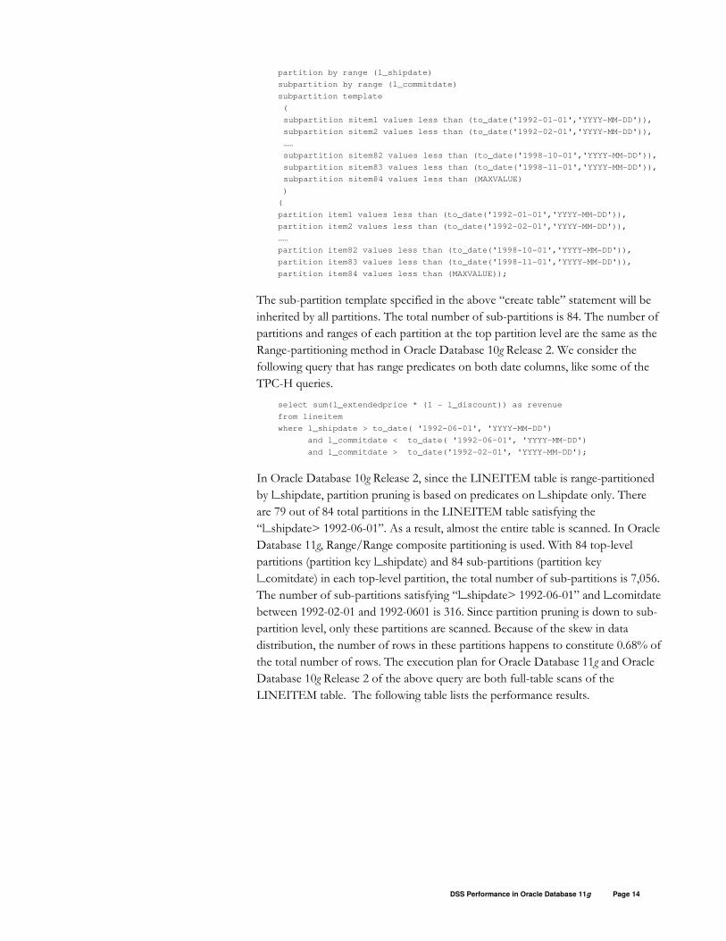
The sub-partition template specified in the above “create table” statement will be
inherited by all partitions. The total number of sub-partitions is 84. The number of
partitions and ranges of each partition at the top partition level are the same as the
Range-partitioning method in Oracle Database 10g Release 2. We consider the
following query that has range predicates on both date columns, like some of the
TPC-H queries.
select sum(l_extendedprice * (1 - l_discount)) as revenue
from lineitem
where l_shipdate > to_date( '1992-06-01', 'YYYY-MM-DD')
and l_commitdate < to_date( '1992-06-01', 'YYYY-MM-DD')
and l_commitdate > to_date('1992-02-01', 'YYYY-MM-DD');
In Oracle Database 10g Release 2, since the LINEITEM table is range-partitioned
by l_shipdate, partition pruning is based on predicates on l_shipdate only. There
are 79 out of 84 total partitions in the LINEITEM table satisfying the
“l_shipdate> 1992-06-01”. As a result, almost the entire table is scanned. In Oracle
Database 11g, Range/Range composite partitioning is used. With 84 top-level
partitions (partition key l_shipdate) and 84 sub-partitions (partition key
l_comitdate) in each top-level partition, the total number of sub-partitions is 7,056.
The number of sub-partitions satisfying “l_shipdate> 1992-06-01” and l_comitdate
between 1992-02-01 and 1992-0601 is 316. Since partition pruning is down to sub-
partition level, only these partitions are scanned. Because of the skew in data
distribution, the number of rows in these partitions happens to constitute 0.68% of
the total number of rows. The execution plan for Oracle Database 11g and Oracle
Database 10g Release 2 of the above query are both full-table scans of the
LINEITEM table. The following table lists the performance results.
DSS Performance in Oracle Database 11g Page 15
Elapsed Time (s) Data Read (MB)
Oracle Database 10g Release 2 153 23234
Oracle Database 11g 2.28 183
With the range partitioning strategy in Oracle Database 10g Release 2, the query
accesses about 23 GB data after partition pruning based on the “l_shipdate”
predicate. Among the 23 GB of data scanned, only a small subset of the data that
satisfies the “l_commitdate” predicates is used to compute the query result. With
the range/range partitioning method in Oracle Database 11g, the additional
partition pruning based on both the “l_shipdate” and “l_commitedate” predicates
enables the query to access only 183 MB of data. All of this data is used to
compute the query result.
Oracle Database 10g Release 2 takes 153 seconds to scan the 23 GB of data and to
compute the query result using a small subset of the scanned data. Oracle database
11g takes 2.28 seconds to scan 183 MB of data and to aggregate all of the scanned
rows to get the query result. Oracle Database 11g is about 70 times faster than
Oracle Database 10g Release 2 in terms of elapsed time.
DSS queries on very large tables present special performance challenges because
queries that require a table scan can take a long time. These additional composite
partitioning methods in Oracle Database 11g help address this DSS performance
challenge by enabling additional partition pruning to be used in many queries.
FULL OUTER JOIN
An “inner” join finds values of two tables that are in a relation to each other. A
row whose column-value is not found in the other table's joined column is not
returned at all. However, sometimes, there is a requirement to show these rows as
well. A left (right) outer join will return all the rows that an inner join returns plus
one row for each of the other rows in the first (second) table that did not have a
match in the second (first) table. A full outer join acts as a combination of the left
and right outer joins. In addition to the inner join, rows from both tables that have
not been returned in the result of the inner join are preserved and extended with
NULLs.
Oracle Database 10g Release 2 does not have native support for the full outer join2.
The ANSI specification of the full outer join is internally converted into a UNION
ALL query. Oracle Database 11g provides native support for the full outer join
using a hash-based method. Existing hash joins are augmented to efficiently handle
2 Oracle Database 10g Release 2, 10.2.0.3 enables native support for the full outer join using an underscore parameter.
DSS Performance in Oracle Database 11g Page 16
the full outer join. The native approach can be utilized if the following conditions
are met:
• At least one join condition is an equi-join.
• Join conditions should be ANDed together, e.g., P1.a = P2.a and (p1.b > p2.b or p1.c < p2.c).
• There are no sub queries on the join conditions.
• There is no correlation in the join conditions or in the tables.
As an example, we consider the following query that joins tables P1, P2, and P3
using a full outer join. Table P1 contains the “quantity sold” and “amount sold”
information for different products in period 1. Table P2 contains the “quantity
sold” and “amount sold” information for different products in period 2.
Table P3 is the result of an aggregation query over the SALES table. It aggregates
and gets the “amount sold” information for different products in the current
period.
select prod_id, sum(amount_sold) as amount_sold
from sales group by prod_id
Since the products sold in each period do not always match, there may be products
sold in one period but not in another period. The following query lists the
“amount sold” information for different products from period 1, period 2, and the
current period. To avoid outputting many rows, the query is wrapped with a select
count(*) at top level. Examination of query execution plan shows that the added
“select count(*)” does not change the underlying query’s execution plan in both
Oracle Database 10g Release 2 and Oracle Database 11g.
select count(*) from
(select
p1.amount_sold a, p2.amount_sold b, p3.amount_sold c
from
( p1 full outer join p2
on p1.prod_id=p2.prod_id
full outer join
( select prod_id, sum(amount_sold) as amount_sold
from sales group by prod_id
) p3
on p1.prod_id = p3.prod_id and p2.prod_id = p3.prod_id
)
);
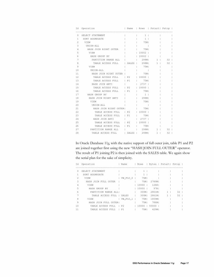
In Oracle Database 10g Release 2, the optimizer converts the two full outer joins in
the query into two UNION ALLs. As a result of the conversion, tables are
accessed multiple times. The execution plan for Oracle Database 10g Release 2 is
listed below. The query was run in parallel, but for the sake of simplicity we show
the serial plan that has the same execution logic as the parallel plan.
DSS Performance in Oracle Database 11g Page 17
Id Operation | Name | Rows | Pstart| Pstop |
------------------------------------------------------------------
0 SELECT STATEMENT | | 1 | | |
1 SORT AGGREGATE | | 1 | | |
2 VIEW | | 75M| | |
3 UNION-ALL | | | | |
4 HASH JOIN RIGHT OUTER | | 75M| | |
5 VIEW | | 10002 | | |
6 HASH GROUP BY | | 10002 | | |
7 PARTITION RANGE ALL | | 298M| 1 | 32 |
8 TABLE ACCESS FULL | SALES | 298M| 1 | 32 |
9 VIEW | | 75M| | |
10 UNION-ALL | | | | |
11 HASH JOIN RIGHT OUTER | | 75M| | |
12 TABLE ACCESS FULL | P2 | 10000 | | |
13 TABLE ACCESS FULL | P1 | 75M| | |
14 HASH JOIN ANTI | | 2737 | | |
15 TABLE ACCESS FULL | P2 | 10000 | | |
16 TABLE ACCESS FULL | P1 | 75M| | |
17 HASH GROUP BY | | 1 | | |
18 HASH JOIN RIGHT ANTI | | 298M| | |
19 VIEW | | 75M| | |
20 UNION-ALL | | | | |
21 HASH JOIN RIGHT OUTER| | 75M| | |
22 TABLE ACCESS FULL | P2 | 10000 | | |
23 TABLE ACCESS FULL | P1 | 75M| | |
24 HASH JOIN ANTI | | 2737 | | |
25 TABLE ACCESS FULL | P2 | 10000 | | |
26 TABLE ACCESS FULL | P1 | 75M| | |
27 PARTITION RANGE ALL | | 298M| 1 | 32 |
28 TABLE ACCESS FULL | SALES | 298M| 1 | 32 |
In Oracle Database 11g, with the native support of full outer join, table P1 and P2
are joined together first using the new “HASH JOIN FULL OUTER” operator.
The result of P1 joining P2 is then joined with the SALES table. We again show
the serial plan for the sake of simplicity.
Id Operation | Name | Rows | Bytes | Pstart| Pstop |
-------------------------------------------------------------------------
0 SELECT STATEMENT | | 1 | | | |
1 SORT AGGREGATE | | 1 | | | |
2 VIEW | VW_FOJ_0 | 75M| | | |
3 HASH JOIN FULL OUTER | | 75M| 2789M| | |
4 VIEW | | 10000 | 126K| | |
5 HASH GROUP BY | | 10000 | 97K| | |
6 PARTITION RANGE ALL| | 300M| 2861M| 1 | 32 |
7 TABLE ACCESS FULL | SALES | 300M| 2861M| 1 | 32 |
8 VIEW | VW_FOJ_1 | 75M| 1859M| | |
9 HASH JOIN FULL OUTER| | 75M| 786M| | |
10 TABLE ACCESS FULL | P2 | 10000 | 50000 | | |
11 TABLE ACCESS FULL | P1 | 75M| 429M| | |
DSS Performance in Oracle Database 11g Page 18
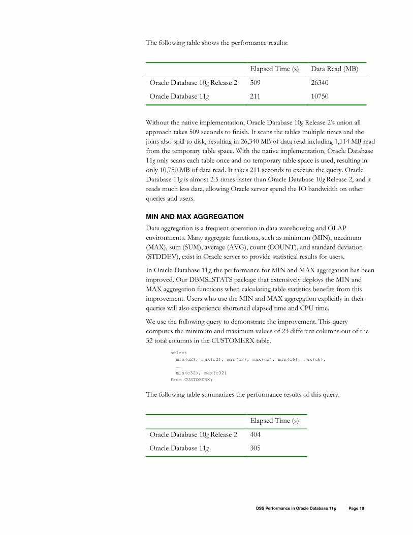
The following table shows the performance results:
Elapsed Time (s) Data Read (MB)
Oracle Database 10g Release 2 509 26340
Oracle Database 11g 211 10750
Without the native implementation, Oracle Database 10g Release 2’s union all
approach takes 509 seconds to finish. It scans the tables multiple times and the
joins also spill to disk, resulting in 26,340 MB of data read including 1,114 MB read
from the temporary table space. With the native implementation, Oracle Database
11g only scans each table once and no temporary table space is used, resulting in
only 10,750 MB of data read. It takes 211 seconds to execute the query. Oracle
Database 11g is almost 2.5 times faster than Oracle Database 10g Release 2, and it
reads much less data, allowing Oracle server spend the IO bandwidth on other
queries and users.
MIN AND MAX AGGREGATION
Data aggregation is a frequent operation in data warehousing and OLAP
environments. Many aggregate functions, such as minimum (MIN), maximum
(MAX), sum (SUM), average (AVG), count (COUNT), and standard deviation
(STDDEV), exist in Oracle server to provide statistical results for users.
In Oracle Database 11g, the performance for MIN and MAX aggregation has been
improved. Our DBMS_STATS package that extensively deploys the MIN and
MAX aggregation functions when calculating table statistics benefits from this
improvement. Users who use the MIN and MAX aggregation explicitly in their
queries will also experience shortened elapsed time and CPU time.
We use the following query to demonstrate the improvement. This query
computes the minimum and maximum values of 23 different columns out of the
32 total columns in the CUSTOMERX table.
select
min(c2), max(c2), min(c3), max(c3), min(c6), max(c6),
……
min(c32), max(c32)
from CUSTOMERX;
The following table summarizes the performance results of this query.
Elapsed Time (s)
Oracle Database 10g Release 2 404
Oracle Database 11g 305
DSS Performance in Oracle Database 11g Page 19
With the new optimized code path for MIN and MAX aggregation, running the
query in Oracle Database 11g is 1.3 times faster than running the query in Oracle
Database 10g Release 2.
NESTED LOOP JOIN
To join two tables through a Nested Loop join, the Oracle Optimizer first selects
one table as outer table and the other as inner table. The Oracle Database server
then scans the outer table row by row and for each row in the outer table, it scans
the inner table, looking for matching rows. A Nested Loop join will be chosen if
one of the tables is small and the other table has an index on the column that joins
the tables. The smaller table is usually the outer table. For each row in the smaller
table scanned, the other table can be probed via an index on the join column. As a
result, we often see operations like TABLE ACCESS BY INDEX ROWID,
UNIQUE INDEX LOOKUP and INDEX RANGE SCAN in Nested Loop join
execution plan.
These operations often generate many random I/O requests. For example, with
“TABLE ACCESS BY INDEX ROWID”, the database could access a large
number of rows using a poorly clustered B-tree index. Each row accessed by the
index would likely be in a separate data block and thus would require a separate
I/O operation. Since the I/Os are spread throughout the table, the buffer cache
hit ratio is low. In such cases, a query can easily become I/O bound, waiting for
single data blocks to be read into the cache one at a time, even though there may
be available I/O bandwidth on the system. In the case that index’s branches or leaf
blocks are not in buffer cache, “UNIQUE INDEX LOOKUP” may generate even
more random I/O because each index lookup requires several random block gets,
one at each B-Tree index level. Short INDEX RANGE SCAN is very similar to
UNIQUE INDEX LOOKUP as far as the I/O latency is concerned. As a result, a
Nested Loop join can often wait for random I/O (I/O for data blocks or index
blocks) to be completed. We call these Nested Loop joins random IO latency
bound.
To reduce the random I/O latency for both index blocks and data blocks during
the process of these Nested Loop joins, Oracle Database 11g buffers random I/O
requests until multiple data or index blocks are ready to be accessed, and then
issues array read (vectored I/O) to retrieve the multiple data blocks or index
blocks at once, rather than reading a single block at a time. This new approach
allows I/O requests for index blocks, in addition to data blocks, to be buffered.
The existing data block pre-fetching method (buffering data block I/O requests
from “TABLE ACCESS BY INDEX ROWID” operation) is also optimized for
the case of Nested Loop join to decrease the memory and CPU cost of buffering
I/O requests.
Buffering I/O requests and issuing array reads allow better utilization of the I/O
capacity because I/O operations are issued in parallel whenever possible. Issuing
DSS Performance in Oracle Database 11g Page 20
one system call for multiple I/O requests, rather than making one system call for
each I/O requests, also decreases the total number of system calls the database
makes, decreasing the total number of context switches. All these provide a further
reduction in response time. Waiting much less often for an I/O to complete helps
the database instance better utilize the CPU resources.
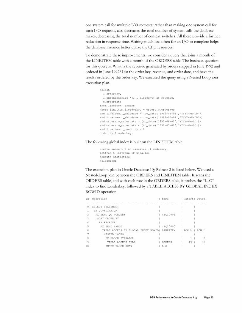
To demonstrate these improvements, we consider a query that joins a month of
the LINEITEM table with a month of the ORDERS table. The business question
for this query is: What is the revenue generated by orders shipped in June 1992 and
ordered in June 1992? List the order key, revenue, and order date, and have the
results ordered by the order key. We executed the query using a Nested Loop join
execution plan.
select
l_orderkey,
l_extendedprice *(1-l_discount) as revenue,
o_orderdate
from lineitem, orders
where lineitem.l_orderkey = orders.o_orderkey
and lineitem.l_shipdate > (to_date('1992-06-01','YYYY-MM-DD'))
and lineitem.l_shipdate < (to_date('1992-07-01','YYYY-MM-DD'))
and orders.o_orderdate > (to_date('1992-06-01','YYYY-MM-DD'))
and orders.o_orderdate < (to_date('1992-07-01','YYYY-MM-DD'))
and lineitem.l_quantity > 0
order by l_orderkey;
The following global index is built on the LINEITEM table.
create index L_O on lineitem (l_orderkey)
pctfree 5 initrans 10 parallel
compute statistics
nologging;
The execution plan in Oracle Database 10g Release 2 is listed below. We used a
Nested-Loop join between the ORDERS and LINEITEM table. It scans the
ORDERS table, and with each row in the ORDERS table, it probes the “L_O”
index to find l_orderkey, followed by a TABLE ACCESS BY GLOBAL INDEX
ROWID operation.
Id Operation | Name | Pstart| Pstop
-------------------------------------------------------------------------
0 SELECT STATEMENT | | |
1 PX COORDINATOR | | |
2 PX SEND QC (ORDER) | :TQ10001 | |
3 SORT ORDER BY | | |
4 PX RECEIVE | | |
5 PX SEND RANGE | :TQ10000 | |
6 TABLE ACCESS BY GLOBAL INDEX ROWID| LINEITEM | ROW L | ROW L
7 NESTED LOOPS | | |
8 PX BLOCK ITERATOR | | 1 | 8
9 TABLE ACCESS FULL | ORDERS | 49 | 56
10 INDEX RANGE SCAN | L_O | |

DSS Performance in Oracle Database 11g Page 21
The execution plan in Oracle Database 11g is:
Id Operation | Name | Pstart| Pstop
--------------------------------------------------------------------------
0 SELECT STATEMENT | | |
1 PX COORDINATOR | | |
2 PX SEND QC (ORDER) | :TQ10001 | |
3 SORT ORDER BY | | |
4 PX RECEIVE | | |
5 PX SEND RANGE | :TQ10000 | |
6 NESTED LOOPS | | |
7 NESTED LOOPS | | |
8 PX BLOCK ITERATOR | | 1 | 8
9 TABLE ACCESS FULL | ORDERS | 49 | 56
10 INDEX RANGE SCAN | L_O | |
11 TABLE ACCESS BY GLOBAL INDEX ROWID| LINEITEM | ROWID| ROWID
The changed plan presentation in Oracle Database 11g indicates the deployment of
the new array-read approach. The new approach provides transparent performance
improvement for the query, as indicated in the table below.
Elapsed Time (s) # Read Requests /s
Oracle Database 10g Release 2 368 1117
Oracle Database 11g 127 3352
In Oracle Database 10g Release 2, this query takes 368 seconds to finish. The query
was IO-bound. The buffering and array-read approach in Oracle Database 11g
effectively decreases the IO latency for read requests, enabling Oracle server to
service 3352 read requests per second. This significantly brings down the elapsed
time of this IO latency bound query down to 127 seconds. Oracle Database 11g is
about 3 times faster than Oracle Database 10g Release 2 for this query.
DBMS_STATS PACKAGE IMPROVEMENTS – NDV
The Oracle cost-based optimizer chooses an optimum execution plan for a SQL
statement based on statistics about the underlying data that the SQL statement
accesses. To get the best execution plan for the SQL statement, it is crucial that the
statistics reflect the state of the data as accurately as possible. It is also important
that the statistics are deterministic. Gathering statistics multiple times on the same
data should yield the same results, otherwise we may have an unstable query
execution plan.
One of the important statistics that the Oracle Optimizer uses is the number of
distinct values of columns in a table (abbreviated as NDV). When histograms are
not available, NDV is used by the Oracle Optimizer to evaluate the selectivity of a
predicate on a column. To get an accurate and deterministic NDV for columns (c1,
c2, etc.) in a table (T), one could certainly issue a SQL statement, such as “select
count(distinct c1), count(distinct c2), .. from T”; however, such a method is
DSS Performance in Oracle Database 11g Page 22
inefficient if the underlying table T is large. The sort generated by such a query
running over large tables could easily spill to disk, resulting in huge temporary
space usage. Therefore, an accurate, deterministic, yet efficient method of NDV
computation is a challenging task.
In Oracle Database 10g Release 2, a sampling-based approach is used by the
DBMS_STATS package to get the NDV statistics of a table. Since the base table is
sampled, no bound exists on the error of the estimation. If a column has lots of
NULLs or the distribution of the column values is skewed, the NDV of the
column may be inaccurate. The sampling-based approach is also not guaranteed to
be deterministic.
Oracle Database 11g provides a new hash-based algorithm in the DBMS_STATS
package to compute NDV. The new algorithm scans the entire table, instead of
sampling the table, in a similar time to that of a sampling. The NDV results
computed by the algorithm are deterministic from run to run, leading to a stable
query execution plan. The algorithm can be used to collect statistics for both non-
partitioned tables and partitioned tables.
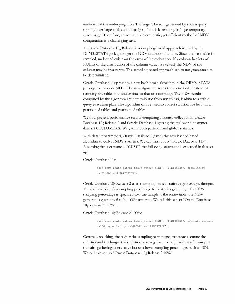
We now present performance results comparing statistics collection in Oracle
Database 10g Release 2 and Oracle Database 11g using the real-world customer
data set CUSTOMERX. We gather both partition and global statistics.
With default parameters, Oracle Database 11g uses the new hashed based
algorithm to collect NDV statistics. We call this set up “Oracle Database 11g”.
Assuming the user name is “CUST”, the following statement is executed in this set
up:
Oracle Database 11g:
exec dbms_stats.gather_table_stats('CUST', 'CUSTOMERX', granularity
=>'GLOBAL and PARTITION');
Oracle Database 10g Release 2 uses a sampling-based statistics gathering technique.
The user can specify a sampling percentage for statistics gathering. If a 100%
sampling percentage is specified, i.e., the sample is the entire table, the NDV
gathered is guaranteed to be 100% accurate. We call this set up “Oracle Database
10g Release 2 100%”.
Oracle Database 10g Release 2 100%:
exec dbms_stats.gather_table_stats('CUST', 'CUSTOMERX', estimate_percent
=>100, granularity =>'GLOBAL and PARTITION');
Generally speaking, the higher the sampling percentage, the more accurate the
statistics and the longer the statistics take to gather. To improve the efficiency of
statistics gathering, users may choose a lower sampling percentage, such as 10%.
We call this set up “Oracle Database 10g Release 2 10%”.
DSS Performance in Oracle Database 11g Page 23
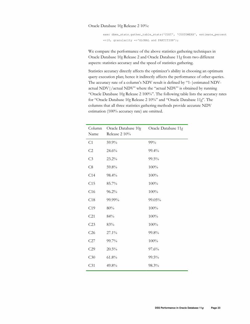
Oracle Database 10g Release 2 10%:
exec dbms_stats.gather_table_stats('CUST', 'CUSTOMERX', estimate_percent
=>10, granularity =>'GLOBAL and PARTITION');
We compare the performance of the above statistics gathering techniques in
Oracle Database 10g Release 2 and Oracle Database 11g from two different
aspects: statistics accuracy and the speed of statistics gathering.
Statistics accuracy directly affects the optimizer’s ability in choosing an optimum
query execution plan; hence it indirectly affects the performance of other queries.
The accuracy rate of a column’s NDV result is defined by “1-|estimated NDV-
actual NDV|/actual NDV” where the “actual NDV” is obtained by running
“Oracle Database 10g Release 2 100%”. The following table lists the accuracy rates
for “Oracle Database 10g Release 2 10%” and “Oracle Database 11g”. The
columns that all three statistics gathering methods provide accurate NDV
estimation (100% accuracy rate) are omitted.
Column
Name
Oracle Database 10g
Release 2 10%
Oracle Database 11g
C1 59.9% 99%
C2 24.6% 99.4%
C3 23.2% 99.5%
C8 59.8% 100%
C14 98.4% 100%
C15 85.7% 100%
C16 96.2% 100%
C18 99.99% 99.05%
C19 80% 100%
C21 84% 100%
C23 83% 100%
C26 27.1% 99.8%
C27 99.7% 100%
C29 20.5% 97.6%
C30 61.8% 99.5%
C31 49.8% 98.3%
DSS Performance in Oracle Database 11g Page 24
Because of the skewed data distribution for many columns in the CUSTOMERX
table, “Oracle Database 10g Release 2 10%” gives inaccurate NDV estimation in
many cases. The accuracy rate ranges from 20.5% to 100%. The new hash-based
Algorithm in “Oracle Database 11g” generates highly accurate statistics, regardless
whether the columns are skewed or not. The accuracy rate for the Oracle Database
11g method ranges from 97.6% to 100%.
The second aspect of the comparison between Oracle Database 10g Release 2 and
Oracle Database 11g is the speed of statistics gathering. The following table
compares elapsed time between Oracle Database 10g Release 2 and Oracle
Database 11g when gathering statistics for the CUSTOMERX table:
Elapsed Time (s)
Oracle Database 10g Release 2 10% 2155
Oracle Database 10g Release 2 100% 24242
Oracle Database 11g 1516
“Oracle Database 10g Release 2 100%” takes the longest time, 24242 seconds, to
finish. The sort operation generated by the “count(distinct)” spilled to disk,
generating 12 GB temporary space usage. With 10% sampling size, Oracle
Database 10g Release 2 finishes much faster, within 2155 seconds. The hash-based
algorithm in Oracle Database 11g, takes only 1516 seconds. Oracle Database 11g is
about 16 times faster than “Oracle Database 10g Release 2 100%”.
Oracle Database 11g has improved DBMS_STATS package significantly by
introducing the new algorithm to compute column NDV. The statistics accuracy
delivered by the new algorithm is close to gathering statistics on the full data set
(Oracle Database 10g Release 2 100%). The performance of the new algorithm is
competitive to sampling based methods in Oracle Database 10g Release 2.
INCREMENTAL MAINTENANCE OF NDV FOR PARTITIONED TABLE
For partitioned tables, Oracle maintains statistics at two different levels, partition
level (called partition statistics) and table level (called global statistics.) Both the
partition statistics and global statistics are important for the optimizer in choosing
optimum execution plans for queries accessing partitioned tables.
Partition statistics are useful because of the partition pruning technique. Given a
SQL statement, the Oracle Query Optimizer will eliminate (i.e., prune) unnecessary
partitions from access by the SQL statement. For example, consider the following
statement accessing LINEITEM table partitioned by partition key l_shipdate:

DSS Performance in Oracle Database 11g Page 25
select *
from lineitem
where l_shipdate between ‘2006-06-01’ and ‘2006-07-01’
and tax > 10000;
This statement will only access the data in the June 2006 partition. Once the
optimizer decides the partitions to be accessed, the statistics on these partitions
can help choosing the right plan. In this example, the optimizer relies on partition
statistics to estimate the selectivity of the predicate “tax > 10000” in the June
partition to choose between a table scan and any possible index accesses.
For some other queries that have no predicates on the partition key, for example,
select *
from lineitem
where tax>30;
partition pruning techniques can not be applied to eliminate the number partitions
accessed by the query. In these cases, global statistics will be used by Oracle Query
Optimizer to select the optimum query execution plan.
Most global statistics gathered by Oracle objects (tables, indexes, etc) can be
derived from partition statistics. These include the number of rows, the number of
blocks, average row length, the number of NULL values, maximum and minimum
values, etc. For example, the global number of NULL values in a column is the
sum of number of NULL values in each partition. The only exception is the global
number of distinct values (abbreviated as NDV). Let’s consider a table T with two
partitions P1 and P2. Column c in this table has 10 and 20 distinct values in P1 and
P2 respectively. The number of distinct values for the entire table T may range
from 20 (when the domain of c in P1 is a subset of that in P2) to 30 (when the
domain of c in P1 does not intersect with that in P2).
In order to get accurate NDV at both partition level and global level, Oracle
Database 10g Release 2 uses a two–pass statistics gathering method. Each partition
is scanned once to gather the partition statistics. All partitions will be scanned
again to gather the global statistics. In other words, partition statistics and global
statistics are gathered independently of each other. This means that when data
changes in some partitions, not only do we need to re-gather statistics on the
changed partitions, but also we have to scan the entire table to gather global
statistics.
In Oracle Database 11g, getting accurate NDV at both the partition level and the
global level for partitioned tables can be done in a one-pass process e. First, the
new hash-based algorithm is used to gather partition level NDV and generate
synopses or summaries for each partition. Then global NDV can be obtained by
aggregating all the synopses at partition level. When data changes in some
partitions, Oracle Database 11g only re-gathers the statistics for the changed
partitions to get new synopses. Since the synopses on the unchanged partitions

DSS Performance in Oracle Database 11g Page 26
remain the same, the global statistics can be derived based on the new synopses of
the changed partitions and the old synopses of unchanged partitions. This
incremental maintenance of NDV allows the database to obtain global statistics
after changes happen without scanning the entire table, significantly improving the
performance of statistics gathering.
We demonstrate the incremental maintenance of statistics for a partitioned table
using the CUSTOMERX table. The CUSTOMERX table contains 10 partitions
but the last partition was empty initially. After gathering statistics for the table, we
load new data, 1000 rows, into the empty partition. We measure the performance
of the statistics maintenance after the data load. The incremental maintenance in
Oracle Database 11g is compared with the following two approaches in Oracle
Database 10g Release 2:
The first approach is to issue the “gather_table_stats” command with granularity
set to “GLOBAL and PARTITION” after the data load. This will re-gather global
statistics and partition statistics for both the changed and unchanged partitions.
We call this approach “Oracle Database 10g Release 2 10%”.
Oracle Database 10g Release 2 10%:
exec dbms_stats.gather_table_stats('CUST', 'CUSTOMERX', estimate_percent
=>10, granularity =>'GLOBAL and PARTITION');
The second approach in Oracle Database 10g Release 2 is to manually gather
partition statistics for the newly loaded partition and then re-gather global
statistics. We call this approach “Oracle Database 10g Release 2 10% Manual”.
Oracle Database 10g Release 2 10% Manual:
exec dbms_stats.gather_table_stats('CUST', 'CUSTOMERX', 'PART10',
estimate_percent =>10, granularity =>'PARTITION')
exec dbms_stats.gather_table_stats('CUST', 'CUSTOMERX', estimate_percent
=>10, granularity =>'GLOBAL')
In Oracle Database 11g, if the INCREMENTAL value for CUSTOMERX table is
set by using DBMS_STATS.SET_TABLE_PREF procedure, Oracle will only re-
gather statistics on the newly loaded partition and derive global statistics from the
new statistics on the changed partition and existing statistics on the unchanged
partitions. We call this approach “Oracle Database 11g Incremental”.
Oracle Database 11g Incremental:
exec dbms_stats.set_table_prefs('CUST', 'CUSTOMERX', 'INCREMENTAL',
'TRUE');
exec dbms_stats.gather_table_stats(‘CUST', 'CUSTOMERX', granularity
=>'GLOBAL and PARTITION');
The following table shows the performance results for these three methods.

DSS Performance in Oracle Database 11g Page 27
Elapsed Time (s)
Oracle Database 11g Incremental 1.25
Oracle Database 10g Release 2 10% 2152
Oracle Database 10g Release 2 10% Manual 1058
With incremental maintenance of statistics in Oracle Database 11g, we only need to
re-gather the statistics on the newly loaded partition. The global statistics are
derived from the new statistics on the changed partition and existing statistics on
the unchanged partition. The elapsed time is only 1.25 seconds. In contrast,
without the incremental maintenance functionality in Oracle Database 10g Release
2, the statistics need to be collected on the entire table. The first approach “Oracle
Database 10g Release 2 10%” re-gathers all the partition statistics and global
statistics. It takes 2152 seconds. The second approach “Oracle Database 10g
Release 2 10% Manual” only re-gathers global statistics and the partition statistics
for the newly loaded partition. This takes 1058 seconds. In summary, Oracle
Database 11g is orders of magnitude faster than Oracle Database 10g Release 2 in
this example.
The incremental maintenance of statistics for partitioned tables demonstrated in
this section is very useful for DSS applications. In this area, data is often
partitioned, and is mostly read-only. When modifications occur, either only a few
partitions (most likely the most recent ones) are updated or new partitions are
added. As we have shown through examples using real world customer data, the
new incremental statistics maintenance mechanism in Oracle Database 11g
dramatically improves the performance of statistics maintenance for partitioned
tables.
CONCLUSION
Due to the growing sizes of data warehouses today there is an ongoing need for
improved performance. This paper shows that Oracle Database 11g provides new
features and enhancements that can significantly improve the performance of DSS
applications.
DSS Performance in Oracle Database 11g
August 2007
Author: Linan Jiang
Contributing Authors: Mark Van de Wiel
Oracle Corporation
World Headquarters
500 Oracle Parkway
Redwood Shores, CA 94065
U.S.A.
Worldwide Inquiries:
Phone: +1.650.506.7000
Fax: +1.650.506.7200
oracle.com
Copyright © 2007, Oracle. All rights reserved.
This document is provided for information purposes only and the
contents hereof are subject to change without notice.
This document is not warranted to be error-free, nor subject to any
other warranties or conditions, whether expressed orally or implied
in law, including implied warranties and conditions of merchantability
or fitness for a particular purpose. We specifically disclaim any
liability with respect to this document and no contractual obligations
are formed either directly or indirectly by this document. This document
may not be reproduced or transmitted in any form or by any means,
electronic or mechanical, for any purpose, without our prior written permission.
Oracle, JD Edwards, and PeopleSoft are registered trademarks of
Oracle Corporation and/or its affiliates. Other names may be trademarks
of their respective owners.


![What to expect from a QSA assessment.ppt [Read-Only] · 2016. 2. 26. · Some Characteristics of PCI DSS Some attributes of the PCI DSS that can be used to compare it to other standards](https://static.documents.pub/doc/80x56/5fbead6b6dd15063c642f3b6/what-to-expect-from-a-qsa-read-only-2016-2-26-some-characteristics-of-pci.jpg)


