OTIC

HITTING LINES WITH TWO-DIMENSIONAL

BROWNIAN MOTION~AccqSSion ForBY NT I GRIDTIC

TAB

SATISH IYENGAR Unannounced

D;]Justificatio

Dstrlbut -.,ntib t n/

TECHNICAL REPORT NO . 429 --i-- i-- t - &

Availabilty Codes

MAY 27, 1990

Prepared Under Contract I L

N00014-89-J-1627 (NR-042-267)

For the Office of Naval Research

Herbert Solomon, Project Director

Reproduction in Whole or in Part is Permittedfor any purpose of the United States Government

Approved for public release; distribution unlimited.

DEPARTMENT OF STATISTICS

STANFORD UNIVERSITY

STANFORD, CALIFORNIA

1. Introduction

rris paper consists of the computation of several hitting time and hitting

place dist;ibUtions for two-dimensional Brownian motion. The motivation for this

study is two-fold: first, to get a diffusion model for the firing behavior of

a simple network of neurons, and second, to get an interesting two-dimensional ver-

sion of the inverse Gaussian distribution. -' [K

Fienberg (1974) has reviewed various models for the firing of single neurons.

A classical model of Gerstein and Mandelbrot C1964) says that if the electrical

state (or potential) of the neural membrane is specified by a single number,

which moves towards or away from the firing potential as the neuron receives ex-

citatory or inhibitory input, resp., then the time to firing can be approximated

by the first hitting time of a certain level for a Brownian motion with drift.

The authors showed that this model could be used to provide a satisfactory fit to

some data that they observed; more importantly, they showed by Monte Carlo methods

that neural activity in the presence of stimuli could also be well duplicated by

a modification of the above random walk model.

Next, the review by Folks and Chhikara (1978) shows that the inverse Gaussian

distribution has many nice statistical properties which, to a large extent mirror

those of the Gaussian distribution. It is natural, then, to ask whether there

is a multivariate inverse Gaussian whose statistical properties are similar to those

of the multivariate Gaussian.

Several proposals for a bivariate inverse Gaussian have already appeared in

the literature. Barndorff-Nielsen and Blaesild (1983) define reproductive ex-

ponential families and propose a bivariate inverse Gaussian model; they claim that

their generalization has nice statistical properties (i.e., affords tractable

2

estimation and analysis of variance), but their proposal does not have inverse

Gaussian marginals. Wasan (1969, 1972) proposes several bivariate inverse Gaussians

but does not develop their properties.

2. A Simple Neural Network

Consider the three neurons of Figure 1. Neuron A sends predominantly exci-

N B

AC

Figure 1

tatory signals, s, to B and C. B and C share a common noise, n, and they also have

independent sources of noise, n1 and n2, resp. If the electrical states of B

and C are encoded by single numbers, X1 (t) and X2 (t), resp., then Xi(t) has

three components; the common noise n, the particular noise ni, and the signal s.

Let the noise variances be a2 for n and a2 for nj; then it is easy to see thata2 02

- 1/1corr(X t),X 2 t,) (1 + -I )(a + 2

0 0

which is a function of the noise ratios. Also, we may allow the drifts of

X1(t) and X2 (t) (due to the signal, s) to be different since B and C may accept

the same input but integrate it differently. When either Brownian reaches the

3

firing threshold, the appropriate neuron fires, returns to its resting state,

and the process starts afresh. What are of interest, then, are the firing times

or the first hitting times for the Brownian motions. Alternatively, this

model can be used to study a single neuron: if we postualte that the neuron has

two interacting trigger zones, (Gerstein, et al. (1964)), then the components of

the Brownian motion describe the electrical state of each zone. Mathematically,

the two problems are the same.

3. Preliminaries

We start with a correlated driftless Brownian motion X(t) with EX(t) -0

and var X(.t) - t. Here

Io and *I/2 - = cos sin 1P sin cos

where p-sin(20), 18, < Tr/4. Thus X(t) . tl/ 2Z(t) where Z(t) is a standard

Brownian motion: var Z(t)= tI. Also define the two stopping times Ti inf{t: XiWt-a

- inf{t: Z(t) i ). Here ai >0 without loss of generality, and ti is the line

V E 3R2. v.Iq/2 el a a i) and {e,,e 2 ) is the standard basis for R 2 . By the scale

invariance of Brownian motion, we can take a, =1. Finally, by elementary methods,

we arrive at the following problem (see Figure 2): start a Brownian motion at x

W (X ,x2 ) - (rocos 0 ,rosineO), and study the stopping times and places associated

with tI and T2"

4

L1

L2L2

Fi ure 2

Here T is the first hitting time of Lis and ao-E+sin-1 p. Also, let1 2

W - {(r,8): r>0, 0< e<a}, and T' - TEl A -E2 be the first hitting time of W.

Our aim is to get the joint density of (TI1l.2), and on the way we compute other

quantities that are also of interest. In particular, we study the following

quantities:

a) PX(T>t, Z(t) eB), BcW

b) pX(T> t)

c) PX(Z(T' ), A), A c aW

d) PX(Tedt, Z(t) eda), acaW

e) P x(Tl cds, T2 cdt)

f) the above quantities in the presence of drift.

Here P X is the measure associated with standard Brownian motion starting at

x; EX will denote the corresponding expectation. Note that the marginal dis-

tributions of Ti are easy:

x d, and A AP x T 2 dt dtandPX(-r1 dt) - - (-dt

pX( Vt1

5

where A - x1sin -x 2cosa and (x) = (27r)- 1/2 e-x2/2

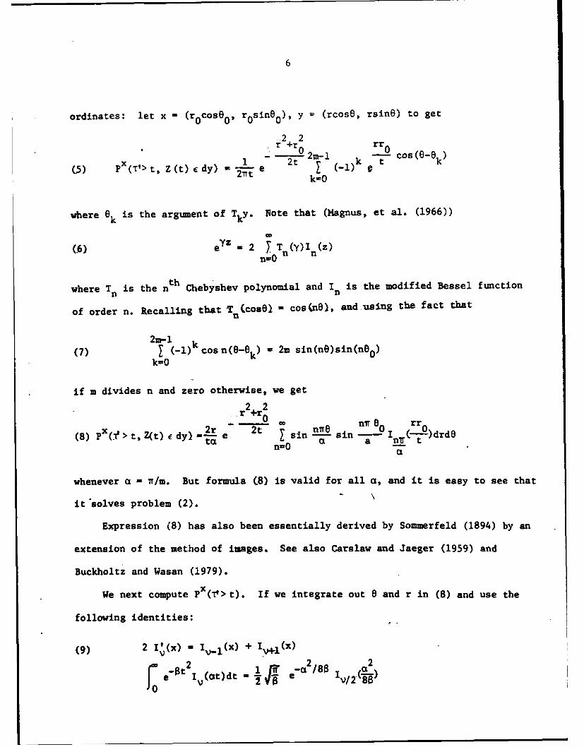
4. Brownian Motion in the Wedge

The main result of this section is contained in (8). Most of the subse-

quent results follow from it. If we have a positive bounded continuous function

f defined on W, and which vanishes on aW, then

(1) u(t,x) - ExfCZ (.T'^ t)) - f(y)PX(> t,Z (t) E dy)

satisfies the heat equation with boundary and initial conditions

(2) ut = Au in W; u(O,x) -f(x), xcW; u(t,z)-0, ze W.t2

We can solve (2) when a = 7/m, m=l,2,... by the method of images. That is,

if we let T -I, Fj be the matrix representing the reflection across the line

y,-xtan and Tj -F oTj_1, and let f(y) - (-l)kf(Tk y) for y cTk(W), we have

the initial value problem

(3) utm-!Au in u(Ox)- f(x), xcm

The solutlon is

-fZt) 2m-i k x-Tky du(t,x) J (~t)-f f(y) k (-1) 02 /-

where 02 (x) - (27)- exp(-x'x/2). It is easy to see that

2m-1 k x-TRky(4) PX(, 1 '> t,Z (t) c dy) F ( - l) .02 -- y.

k= (--tldy

While (4) is appropriate only for the special angles eo - I/m, the following

argument gives us the result in general. To facilitate this, we use polar co-

6

ordinates: let x m (r0cosOO, r0sineo), y = (rcose, rsine) to get

.2 2r +r rr

X 1 0 2m- 1 k 0 cos(e-ek)(.5) p (,> t, Z (t) c dy) - 2-te (-1),k=O

where ek is the argument of TkY. Note that (Magnus, et al. (1966))

(.e e yz . 2 iTn(Y) In(z)

where Tn is the nth Chebyshev polynomial and In is the modified Bessel function

of order n. Recalling that T n(cosl - cos(nO), and using the fact that

2m-1 k(7) 1 (-1) cos n(e-k) 2m sin(nO)sin(n80 )

k=O

if m divides n and zero otherwise, we get

22r+r 0 niT rr

2t0 0()P(Et t)d m2re 2t n sin sin- In- )drd8(8 e(.Y > t, Z(t) c dy) . -Lr e- I sin -7-r si aLPI = dd

tan-0 a a nir ta

whenever a - w/m. But formula (8) is valid for all a, and it is easy to see that

it solves problem (2).

Expression (8) has also been essentially derived by Sommerfeld (1894) by an

extension of the method of images. See also Carslaw and Jaeger (1959) and

Buckholtz and Wasan (1979).

We next compute PX(rl>t). If we integrate out 8 and r in (8) and use the

following identities:

2I'(x) -I

(9) 2 ( = _l(x) + I\4l ( x )

a: 2 =Q 1 2 /88 iv/2(8)e_- I (at)dt 2 e-a

7

(Magnus, et al. (1966)) we get

3r2

2r - 0 co nTre r 2

(10) Px(9e> t)=- e4 . --- in=- {I.,() + I+(-Aif*TI n 4t v+l 4t)

n odd 2 2

where v - ntifo.

When the wedge angle is special- a- I/n- we have the alternate expression

2m-1 k+l k7.(11) P (Y >t 0 2 1 -1

k-0 Dl

where

(12) F(u) - f 0 cos(8-0)R(- - cos(B-80))d.

Here, R is Mills' ratio: R(x) = 0(-x)/l(x), where 4 and * are the normal dis-tribution and density functions, resp. We omit the details of this computation.

The quantity PX ( > t) was also studied by Spitzer (1958), who computed its

transform. Checking the asymptotics of modified Bessel functions, it is easy to

see that Ex(IP- TO Tf-Px(-e>t)dt<ooif and only if cB< ir/2, independent of

X.

The distribution of Z('T' is also of interest. Now u(x;A) - PX U) CA) sat-

isfies Laplace's equation Au - 0 with boundary condition u(x,A) - I{x CA).

The Green's function for the wedge is easily computed, and we have

a7r 1 0(13) PX( Z(TX da) =1 - - sin-- daS ire0 7o) 2 r 0sin2 + (l+cos -0

a at

where we use the plus sign for T2 < T and the minus sign otherwise. Using

elementary estimates, it is easy to see that EX z, (x'texists if f CaB <i, again

Expression (10) corrects a mistake in Wasan and Buckholtz (1979).

8

independent of the initial position, x.

5. Joint distribution of (T T ,

Using an argnent similar to that of Daniels (1982) , it can be shown that

if Px (T > t, Z(t) c dy) - f(t,x,y)dy, then

(14) PX(tc dtZ(T) E da) f - f(t,x,y) I dadt

where--n denotes the derivative in the inward normal direction. See Figure 3.a.

a aa __

Figure 3

When e= O(c), - -r (- r , so from (8) we get

2 22tr0 Gonire ar0

(15) PX(T - dt,ZCT')E da) e 1 2t nsi n - -0 I (12ta n=0 n a nir t

a

where 6n is 1 if e -0 and (-I) n + if e- a. It is clear by symetry that

P X(T'c t,X(T')e da) - pX (c dt, Z(T')e da') where x is the reflection of x across

the line y - x tan .. And for the special angle a - n/m, a simpler. formula is avail-

able:

I thank Professor D. Siegmund for this reference.

9

(16) pX(-r'. d tZCI')4E da)= 2 1)k x2( -) (xY2 e(_l)(x 02Tke 2 )

with PX(TE dt, Z (T'Eda') computed by symmetry.

Finally, we can compute PX( 1 E ds, T2 Edt), the joint density of (T ,T).

By the strong Markov property we have for s <t,

(17) Px(TE d s , T 2 c d t ) f PX(T 1 Eds,ZCT ' )Eda, T2 Edt)

(2 dt).bw

- fWPXCT -eE ds Z(:r-)E da) Pa sina(T2

but the first term of the integrand is given by (15) and the second term is just

(18) Pasina(T2 c d t - s ) f asin (asina)dt,(t-s) /

since T is just a one-dimensional inverse Gaussian. After some computation2

and (9) we get

(19) PX(T I E dsT 2 c dt) -

r2 -n r 0 r0(t-s)/s

7T sincx- 2(t-s)i-(E-s cos 2at 3)~w r0 C-ss2a 2 v(t-s Y -- e (.Ct-s)+(t-s cos 2a) n=Oa __InTr2(t-s)+2t-s Cos a 2ct

Finally, using the fact that (see Figure 3)

pX d d PX( cd(T1E d s , 2 E 1d t ) - P dt, 2 cds), s<t

the joint density of (T1,T 2 ) is determined for s it. In (19) we can let t -s and

10

use the fact that as z- 0, I (z)-(2)/'(v+l) to get

V 2

0 if 0< c,<.!2

(20) PX( I E d s , T Edt) f 2 if < T<r(sig rO0sin2e 0 exp(- ) if = /2

4Ts3 2s

Thus the joint density of (T T 2) is discontinuous on the line s = t only when the

original Brownian motion X(t) is positively correlated. Of course, we could have

started with (16) to get a simpler expression for the joint density of (T1,T2)

for the special angles a = Ir/m; we omit the straightforward calculation.

6. Brownian Motion with. Drift

Of course, the case of Brownian-motion with drift is of more interest. The

analysis, however, is considerably more complicated and so it is not always possi-

ble to evaluate th. integrals that arise. In this section, we extend the results

of the previous sections to Brownian motion with drift.

If, in section 3, the correlated process X(t) has drift e- (e 1 ,e 2 )' where

ei >0, it is easy to see that for the corresponding process Z(t), in the wedge W,

we have drift p - (V' 1 12 ) - (P2-8l, -e2 (lP_2)1 1 /2 Let

(1) f(t;a,b) - b exp- b t-a)

2Tt 3 2a

be the inverse Gaussian density in its usual form 1 6 ,p. 2631. Then it is easy toIx- sin-x cost 2

see that T1 has density f(t, , (X sincr-x 2cosa) 2) and T2 has density

x2 2_-I2 2

2 1-p

11

Let P be the measure associated with uncorrelated Brownian motion starting

at x and with drift U;

2) P 1Z tl)C,.. Z tn) EA n ) = PO (z (t)t 1I.. 1 tn+t n )n

for all n, for all tl<...<tn, and for all Borel sets Ai. Our basic tool is the

exponential (likelihood ratio) martingale

dP x 2(23) -A . exp (pi'(Z (t) -x) -tp /2)

dPx

on Ft , the sigma field generated by Z(t) : s<t}. Thus, we have that

(24) v(t~x,y) - Px(x' >t, Zt)Edy) - ep Y-x)-IV,2t P x'T> t, Z(t)E dy)Pi 0

is a solution to the diffusion equation with convection or drift:

(25) vt -AAv+I'Vv; v(O,x,y) 6 ; v(t,a,y) =0, acaW

where 6 is the Dirac delta. Of course, in (24), Px ' > t, Z t)c dy) is given by

(8). The expressions for Px(T' > t) and F.(Z(T')EA) do not seem to be convenient

as they were for the driftless case ((10) and (13) in section 4), but the joint

density of T' and Z(T') is available. In fact, Daniels' argument gives

(see Figure 3)

(25) P (T'dt,Z(T')Eda) -dtZ )Eda)

00F -x'iw-te2+ hasforsan<_tP(x'cdt,Z(.T )cda') - e /2 a(ilosti iaP0(T".dtz(T')Eda'),

where we use (15) for P (t'cdt,z(r') £da).

Finally, we have for s < t

(27) Px2(TI dsT 2 E dt) f Px(TiEdsZ(Tl)Eda)P asin(T 2 E dt-s).(27) tha PP 1 1dt 2i

Note that P ( dt-s) is just the inverse Gaussian density and

Px (T Eds, z(T 1 ) E da) is given by (21). The integral involved, however, does not

seem to be tractable.

7. Concluding Remarks

Clearly, the .=0 case is much easier than the 100 case; however, the physical

motivation demands 110O. For higher dimensional problems, similar methods can

be used to get the joint distribution of -= (T1,..,T p), where Ti= inf{t>O: Xi(t)=ai},

ai > 0, and X(t) - N(O,t$) is a driftless correlated Brownian motion. The

geometry in Rp is quite complicated though; for certain patterened $ (e.g.,

iJ- p), the transformation to independence can be done in closed form, and the

joint distribution of T is available. The same problem for general t and for

11# 0 requires further investigation, and will be the subject of a subsequent

paper.

13

References

1. Barndorff-Nielsen, 0. and Blaesild, P. (1983). Reproductive ExponentialFamilies. Ann. Stat. vol. 11, 770-782.

2. Buckholtz, P. and Wasan, M. (1979). First Passage Probabilities of a TwoDimensional Brownian Motion in an Anisotropic Medium. Sankhya A vol. 41,198-206.

3. Carslaw, H. and Jaeger, J. (1959). Conduction of Heat in Solids. OxfordUniv. Press.

4. Daniels, H. (1982). Sequential Tests Constructed from Images. Ann. Stat.vol. 10, 394-400.

5. Fienberg, S. (1974). Stochastic Models for Single Neuron Firing Trains:A Survey. Biometrics vol. 30, 399-427.

6. Folks, L. and Chhikara, R. (1978). The Inverse Gaussian Distribution andits Statistical Application - A Review. JRSS B, vol. 40, 263-289.

7. Gerstein, G. and Mandelbrot, B. (1964). Random Walk Models for the SpikeActivity of a Single Neuron. Biophys. J. vol. 4, 41-68.

8. Magnus, W., Oberhettinger, F. and Soni, R. (1966). Formulas and Theorems

for the Special Functions of Mathematical Physics. Springer Verlag.

9. Sommerfeld, A. (1894).Mathematische Annalen. vol. 45, p. 263.

10. Spitzer, F. (1958). Some Theorems Concerning Two Dimensional BrownianMotion. Trans. Amer. Math. Soc. vol. 87. 187-197.

11. W.san, M.T. (1969). First Passage Time Distribution of Brownian Motionwith Positive Drift. Queen's U. Papers on Pure and Applied Mathematics.Fo. 19.

12. Wasan, M.T. (1973). Differential Representation of a Bivariate InverseGaussian Process. J. Mult. Analysis. vol. 3, 243-247.

14

UNCLASSIFIEDSECURITY CLASSIFICATION OF "N:S PAGE (When Date ,ntered)

REPORT DOCUMENTATION PAGE READ INSTRUCTIONSBEFORE COMPLETING FORMI. REPORT NUM8ER 2. GOVT ACCESSION NO. 3. RECIPIENT'S CATALOG NUMMER

429

4. TITLE (and Subtitle) S. TYPE OF REPORT & PERIOD COVERED

Hitting Lines With Two-Dimensional TECHNICAL REPORTBrownian Motion

B. PERFORMING ORG. REPORT NUMBER

7. AUTNOR(s) S. CONTRACT OR GRANT NUMELR(o)

Satish Iyengar N00014-89-J-1627

S. PERFORMING ORGANIZATION NAME AND ArDRESS 10. PROGRAM ELEMENT. PROJECT. TASK

Department of Statistics AREA & WORK UNIT NUMBERS

Stanford University NR-042-267Stanford, CA 94305

,,. CONTROLLING OFFICE NAME AND ADORESS 12. REPORT CATS

Office of Naval Research May 27, 1990

Statistics & Probability Program Code 1111 13. NUMBER OF PAGES16

14. MONITORING AGENCY NAME & AOORESS(tIf dlferent Io Controllng Office) IS. SECURITY CLASS. (of Ulte repert)

UNCLASSIFIED

ISa. OECLASSI FICATION/DOWNGRADINGSCHEDULE

IS. DISTRIBuTION STATEMENT (of thie Report)

APPROVED FOR PUBLIC RELEASE: DISTRIBUTION UNLIMITED

17. DISTRIBUTION STATEMENT (of the abetract &"leed In Sleet 20, If different toam Report)

18. SUPPLEMENTARY NOTES

19. KEY WORDS (Continue an reverse aide It neeeearrN mI fdflirt bW block nMber)

Brownian motion, hitting times and places, inverse Gaussian distribution,

diffusion equation, neural activity.

30, ABSTRACT (Contimne en reverse ilde II neceeeny and Identlo by bleak ImMbea)

PLEASE SEE FOLLOWING PAGE.

DO D , ,r,". 1473 EDITION Of I NOV9 IS OSO.STS

S/N 0102-04-o601 1 UNCLASSIFIED A

L 11CURITY CLASSIFICATION aiF TIS PiAGE t

'0l4on Date WOOt~if

UNCLASSIFIED 15

29CURITY CLASSIPICATION OF T6u1 PAGS (Whom Does £RAe0ew9)

TECHNICAL REPORT NO. 429

20. ABSTRACT

This paper consists of the computation of several hitting time and hitting

place distributions for two-dimensional Brownian motion. The motivation for

this study is two-fold: first, to get a diffusion model for the firing behavior

of a simple network of neurons, and second, to get an interesting two-dimensional

version of the inverse Gaussian distribution.

Several proposals for a bivariate inverse Gaussian have already appeared in

the literature. Barndorff-Nielsen and Blaesild (1983) define reproductive ex-

ponential families and propose a bivariate inverse Gaussian model; they claim

that their generalization has nice statistical properties (i.e., affords tractable

estimation and analysis of variance), but their proposal does not have inverse

Gaussian marginals. Wasan (1969, 1972) proposes several bivariate inverse

Gaussians but does not develop their properties.

SECURITY CLASSIFICATION OP THIS PAOre1a. Do N. Eaet