Dual-Based Approximation Algorithms for Cut-BasedNetwork Connectivity Problems

Benjamin Grimmerbdg79@cornell.edu

Abstract

We consider a variety of NP-Complete network connectivity problems. We intro-duce a novel dual-based approach to approximating network design problems withcut-based linear programming relaxations. This approach gives a 3/2-approximationto Minimum 2-Edge-Connected Spanning Subgraph that is equivalent to a pre-viously proposed algorithm. One well-studied branch of network design models ad hocnetworks where each node can either operate at high or low power. If we allow uni-directional links, we can formalize this into the problem Dual Power Assignment(DPA). Our dual-based approach gives a 3/2-approximation to DPA, improving theprevious best approximation known of 11/7 ≈ 1.57.

Another standard network design problem is Minimum Strongly ConnectedSpanning Subgraph (MSCS). We propose a new problem generalizing MSCS andDPA called Star Strong Connectivity (SSC). Then we show that our dual-basedapproach achieves a 1.6-approximation ratio on SSC. As a consequence of our dual-based approximations, we prove new upper bounds on the integrality gaps of theseproblems.

1 Introduction

In this work, we present approximation algorithms for multiple network connectivity prob-lems. All the problems we consider seek a minimum cost graph meeting certain connectivityrequirements. Problems of this type have a wide array of applications. They have uses in thedesign and modeling of communication and ad hoc networks. Often these problems involvebalancing fault tolerance and connectivity against cost of building and operating a network.

Many standard network connectivity problems have been shown to be NP-Complete [10].As a result, there is little hope of producing fast (polynomial time) algorithms to solvethese problems (unless P = NP ). So the focus has shifted to giving fast (polynomial time)algorithms that approximately solve these problems. An approximation algorithm is said tohave an approximation ratio of α if the cost of its output is always within a factor of α of thecost of the optimal solution. Technically, α can depend on the size of the problem instance,but a constant approximation ratio is better than one that grows.

In Subsections 1.1 and 1.2, we introduce a number of standard graph connectivity prob-lems and their notable approximation algorithms. There are many other connectivity prob-lems and algorithmic tools that we omit from our discussion (See [12] for a more in-depth

1

arX

iv:1

508.

0556

7v2

[cs

.DS]

20

Jul 2

017

survey). Then in Subsection 1.3, we summarize our contributions. In Section 2, we introduceour novel approach to approximating network design problems. The remaining sections willpresent our approximation algorithms based on this methodology.

1.1 Edge-Connectivity Problems

One standard graph connectivity problems is Minimum 2-Edge-Connected SpanningSubgraph (2ECS). This problem takes as input a 2-edge-connected graph and outputsa 2-edge-connected spanning subgraph with minimum cardinality edge set. A 5/4 = 1.25-approximation was proposed using a matching lower bound in [15]. A 4/3 ≈ 1.33-approximationwas given by Vempala and Vetta [23]. Another notable approximation algorithm appearsin [18], which achieves a 1.5 ratio using a graph carving method with linear runtime. Thisgraph carving method is a special case of the dual-based approach we introduce in Section 2.

One can generalize the problem of 2ECS to have weights on every edge. Then the outputis the spanning subgraph with minimum total weight on its edges. This problem seems tobe harder to approximate that the unweighted version. The best approximation known forthe weighted problem was given by Khuller and Vishkin and achieves a 2-approximationin [18]. Later, Jain proposed a 2-approximation that applies to a more general class ofSteiner problems [14].

Another generalization of 2ECS is to search for the k-edge-connected spanning subgraphwith the least number of edges. Using a linear program rounding algorithm, this problemon a multigraph input has a 1 + 3/k-approximation if k is odd and a 1 + 2/k-approximationif k is even [9]. Further, in [9], it is shown that for any fixed integer k ≥ 2 that a (1 + ε)-approximation cannot exist for arbitrary ε > 0 (unless P = NP ).

One of the most fundamental directed graph connectivity problems is Minimum StronglyConnected Spanning Subgraph (MSCS). This problem takes as input a strongly con-nected digraph and outputs a strongly connected spanning subgraph with minimum cardi-nality arc set. In [24], Vetta proposes the best approximation known for MSCS using amatching lower bound to get an approximation ratio of 1.5. There are two other notable ap-proximation algorithms for MSCS. First, Khuller, Raghavachari and Young gave a greedyalgorithm with a 1.61 + ε approximation ratio [16], [17]. Second, Zhao, Nagamochi andIbaraki give an algorithm that runs in linear time with a 5/3 ≈ 1.66-approximation ratioin [27]. This algorithm implicitly uses the dual of the corresponding cut-based linear programto bound the optimal solution.

When MSCS is generalized to have weights on each arc, the best algorithm known isa 2-approximation. This straightforward algorithm works by computing an in-arborescenceand an out-arborescence with the same root in the digraph, and outputting their union. Thisis the best algorithm known even when arc weights are restricted to be in {0, 1}.

1.2 Power Assignment Problems

A well-studied area of network design focuses on the problem of assigning power levels tovertices of a graph to achieve some connectivity property. This is useful in modeling radionetworks and ad hoc wireless networks. It is common in this type of problem to minimizetotal power consumed by the system. This class of problems take as input a directed simple

2

graph G = (V,E) and a cost function c : E → R+. A solution to this problem assignsevery vertex a non-negative power, p(v). We use H(p) to denote the spanning subgraph of Ginduced by the power assignment p (we will formally define H(p) later). The minimizationproblem then is to find the minimum power assignment,

∑p(v), subject to H(p) satisfying

a specific property.The first work on Power Assignment was done by Chen and Huang [8], which assumed

that E is bidirected. We say an instance of Power Assignment is bidirected if wheneveruv ∈ E then vu ∈ E and c(uv) = c(vu). There has been a large amount of interest inthis type of problem since 2000 (some of the earlier papers are [13], [22] and [26]). Whilewe consider problems seeking strong connectivity, other works have focused on designingfault-tolerant networks. In [25], approximations for both problems seeking biconnectivityand edge-biconnectivity are given. Further, [20] considers the more general problems ofk-connectivity and k-edge-connectivity.

We consider an asymmetric version of Power Assignment that allows unidirectional linksdefined as follows. The power assignment induces a spanning directed subgraph H(p) wherexy ∈ E(H(p)) if the arc xy ∈ E and p(x) ≥ c(xy). The goal is to minimize the total powersubject to H(p) being strongly connected. This problem was shown to be NP-Completein [6]. Many different approximations for this problem have been proposed, which are com-pared in [5]. If we assume the input digraph and cost function are bidirected, the bestapproximation known achieves a 1.85-approximation ratio [2].

We are particularly interested in a special case of asymmetric Power Assignment calledDual Power Assignment (DPA). This problem takes a bidirected instance of Asymmet-ric Power Assignment with cost function c : E → {0, 1}. This models a network where eachnode can operate at either high or low power, and finds a minimum sized set of nodes toassign high power to produce a strongly connected network. The best approximation knownfor DPA was proposed by [1] and achieves an 11/7 ≈ 1.57-approximation. This algorithm isbased on interesting properties of Hamiltonian cycles. A greedy approach to approximatingDPA was first given in [7] and achieved a 1.75-approximation ratio. Then in Calinescu in [3]showed that this greedy approach can be extended to match the 1.61+ε-approximation ratioof Khuller et al. for MSCS in [16], [17]. A greedy algorithm based on the same heuristicwas later shown to give a 5/3 ≈ 1.66-approximation with nearly linear runtime in [11].

1.3 Our Results

MSCS and DPA both have approximation algorithms based on very similar ideas. Thisraises the question of how these two problems are related. To answer this question, wepropose a new connectivity problem generalizing both of them called Star Strong Con-nectivity (SSC), defined as follows: We call a set of arcs sharing a source endpoint a star.SSC takes a strongly connected digraph G = (V,E) and a set C of stars as input such that⋃

F∈C F = E. Then SSC finds a minimum cardinality set R ⊆ C such that (V,⋃

F∈R F ) isstrongly connected.

SSC is exactly MSCS when all F ∈ C are restricted to have |F | = 1. Under thisrestriction, choosing any star in SSC would be equivalent to choosing its single arc in MSCS.Further, we make the following claim relating SSC and DPA (proof of this lemma is deferredto Section 3).

3

Lemma 1. When Star Strong Connectivity has a bidirected input digraph G (an arcuv exists if and only if the arc vu exists), it is equivalent to Dual Power Assignment.

In some sense, SSC has a more elegant formulation than DPA. It removes the complexityof having two different classes of arcs. This benefit becomes very clear when constructingInteger Linear Programs for the two problems (our linear programs for SSC and DPA willbe formally introduced in Section 3). Besides this difference in elegance, both the resultingprograms for DPA and SSC constrained to have a bidirected input digraph are equivalentto each other.

We introduce a novel dual-based approach to approximating connectivity problems. Thismethodology utilizes the cut-based linear programming relaxation of a connectivity problem.In Section 2, we give a full description of our approach and apply it to the problem of 2ECS.The resulting algorithm is equivalent to the 3/2-approximation given in [18]. Its value issolely in its simplicity and serving as an example of our approach.

Applying our dual-based method to DPA gives a tight 3/2-approximation. This improvesthe previous best approximation known for DPA of 11/7 ≈ 1.57 [1]. Our algorithm and itsanalysis are made simpler by viewing it as an instance of SSC with a bidirected input digraphinstead of DPA. In Section 3, we present our algorithm, prove its approximation ratio andshow this bound is tight.

Theorem 1. Dual Power Assignment has a dual-based 1.5-approximation algorithm.

Integer Linear Programs are often used to formulate NP-Complete problems. An ap-proximation that uses a linear programming relaxation typically cannot give a better ap-proximation ratio that the ratio between solutions of the integer and relaxed programs. Thisratio is known as the integrality gap of a program. For minimization problems, it is formallydefined as the supremum of the ratio between the optimal integer solution and the optimalfractional solution over all problem instances. As a result of our analysis for Theorem 1, weprove an upper bound of 1.5 for DPA’s integrality gap. This improves the previous upperbound of 1.85 proven in [2].

Corollary 1. The integrality gap of the standard cut-based linear program for Dual PowerAssignment is at most 1.5.

In fact, we prove a slightly stronger statement. Our algorithm constructs integer primaland integer dual solutions. As a result, the gap between integer solutions of these twoproblems is at most 1.5.

Now, we turn our focus to the more general problem of SSC. Our algorithm for DPA isdependent on the underlying digraph being bidirected. Further the 3/2-approximation forMSCS in [24] and 11/7-approximation for DPA in [1] do not seem to generalize to SSC.However the greedy approach used by Khuller et al. in [18] and [16] on MSCS and byCalinescu in [3] on DPA appears to generalize easily to SSC.

Claim 1. SSC has a 1.61 + ε polynomial approximation algorithm using a simple variationof the greedy algorithm of [16].

In Section 4, we improve on this 1.61 + ε-approximation by applying our dual-basedapproach to SSC. This produces an algorithm with a tight 1.6-approximation ratio. Since

4

MSCS is a subproblem of SSC, this approximation ratio also extends to it. As with ourapproximation of DPA, we observe that an upper bound on the integrality gap follows fromour analysis.

Theorem 2. Star Strong Connectivity has a dual-based 1.6-approximation algorithm.

Corollary 2. The integrality gap of the standard cut-based linear program for Star StrongConnectivity (and thus MSCS) is at most 1.6.

Again, we actually prove a slightly stronger statement. Since our algorithm constructsinteger primal and integer dual solutions, the primal-dual integer gap of these two problemsis at most 1.6.

A lower bound on the integrality gap of a problem provides a bound on the qualityof approximation that can be achieved with certain methods. Linear program rounding,primal-dual algorithms, and our dual-based algorithms are all limited by this value. Recently,Laekhanukit et al. proved the integrality gap of MSCS is at least 3/2− ε for any ε > 0 [19].

2 Dual-Based Methodology

In Subsection 2.1, we describe the typical form of integer linear programs (ILPs) related tograph connectivity problems and give a high-level description of our dual-based approach fora general problem. Finally, we apply our dual-based approach to the problem of 2ECS as asimple example.

2.1 Cut-Based Linear Programs

All the connectivity problems considered in this work have cut-based ILPs. In this typeof program, the constraints are based on having at least a certain number of edges or arcscrossing each cut of the graph. We will give the standard cut-based ILP for Minimum 2-Edge-Connected Spanning Subgraph to demonstrate this structure. For a cut ∅ ⊂S ⊂ V , we use ∂E(S) to denote all edges with exactly one endpoint in S. Then the standardcut-based linear programming relaxation for 2ECS is the following.

2ECS Primal LP

minimize∑e∈E

xe

subject to∑

e∈∂E(S)

xe ≥ 2 , ∀∅ ⊂ S ⊂ V

xe ≥ 0 , ∀e ∈ EThe integer programming formulation for 2ECS is given by adding the constraint that

all xe are integer valued. The linear program will always have objective less than or equalto the objective of the integer program.

5

It is worth noting that this type of program has an exponential number of constraints, butit could be converted into a polynomial sized program using flow-based constraints. Previousalgorithms have taken advantage of polynomial time linear program solvers to approximate2ECS using its linear programming relaxation. However, our dual-based algorithms do notneed to solve the linear program. As a result, we can keep it in the simpler cut-based form.

Our method takes advantage of the corresponding dual linear program. The dual programwill always have objective at most that of the original (primal) program. This property isknown as weak duality. In fact, their optimal solutions will have equal objective, but we donot need this stronger property. The dual program corresponding to 2ECS is the following.

2ECS Dual LP

maximize∑∅⊂S⊂V

2yS

subject to∑

e∈∂E(S)

yS ≤ 1 , ∀e ∈ E

yS ≥ 0 , ∀∅ ⊂ S ⊂ V

Since the optimal solution to our integer program is lowerbounded by that of the primallinear program, we know that the optimal integer solution is lowerbounded by every feasiblesolution to the dual program.

The basic idea of our dual-based method is to build a feasible dual solution while con-structing our integer primal solution. We construct our primal solution by repeatedly findingand contracting a problem specific type of subgraph: a cycle for 2ECS, a perfect set for SSC(defined later). Using a cut-based linear program, a dual solution will be a set of disjointcuts (where the exact definition of disjoint is problem specific). We are interested in cutsthat are disjoint from all cuts after contracting a subgraph. Later, we formally define theseas internal cuts. We choose the subgraph to contract based on it having a number of disjointinternal cuts. When our algorithm terminates, the union of these disjoint internal cuts ineach iteration will give a feasible dual solution.

To apply this to a new connectivity problem, we first must define a contractible subgraphsuch that repeated contraction will yield a feasible primal solution. Definitions for disjointand internal cuts will follow from the cut-based program and the contractible subgraphs.Finally, any polynomial runtime procedure that constructs a contractible subgraph withat least one internal cut produces an algorithm creating integer primal and dual solutions.The quality of the approximation depends directly on the number of internal cuts in eachcontraction. Our dual solution could use fractional cuts. However, this did not result inimprovements in the approximation bounds for the problems studied in this paper.

2.2 Application to 2ECS

We will illustrate our dual-based approach by giving a straightforward 3/2-approximation to2ECS. This is neither best known in approximation ratio nor runtime. Its value is to serve

6

as a simple example of our dual-based approach. In [18], an equivalent 3/2-approximationis given for 2ECS that implicitly uses the dual bound. They also show that simple modifi-cations of the algorithm allow it to run in linear time.

Our approximation is based on iteratively selecting and contracting cycles in the graphuntil the graph is reduced to a single vertex (this approach has been used by multiple previousapproximations). We claim that such a procedure will always produce a 2-edge-connectedspanning subgraph. Consider any cut ∅ ⊂ S ⊂ V in the graph. At some point, we will selecta cycle with vertices in both S and V \ S. This cycle must have two edges crossing the cut.Thus such a procedure will always produce a feasible solution.

Consider the primal and dual programs for 2ECS given in Section 2.1. When the dualproblem is restricted to integer values, it can be thought of as choosing a set of cuts suchthat no two cuts share any edges. Our algorithm builds a solution to this dual problem tolower bound the optimal primal solution.

We say a cut S is internal to a cycle C if all edges in ∂E(S) have both endpointsin the vertices of C. To contract a cycle means to replace all vertices of the cycle witha single supervertex whose edge set is all edges with exactly one endpoint in the cycle.When contracting a cycle, we keep duplicate edges (and thus the resulting structure is a 2-edge-connected multigraph). Contracting a cycle with an internal cut will remove all edgescrossing that cut from the graph. As a result, after repeated contraction of cycles each withan internal cut, the set of all these internal cuts is dual feasible. Following from this, ouralgorithm will find a cycle with an internal cut, add the edges of the cycle to our approximatesolution, contract the vertices of our cycle, and then repeat. Complete description of thisprocess is given in Algorithm 1.

Algorithm 1 Dual-Based Approximation for 2ECS

1: R = ∅2: while |V | 6= 1 do3: Find a cycle C with an internal cut as shown in Lemma 24: Contract the vertices of C into a single vertex5: R := R ∪ E(C)6: end while

Lemma 2. Every 2-edge-connected multigraph has a cycle with an internal cut.

Proof. Let N(v) denote the neighbors of a vertex v. We give a direct construction for a cycleC with a vertex v such that all neighbors of v are in the cycle. Then the cut {v} will beinternal to this cycle. Our construction maintains a path P and repeatedly updates a vertexv to be the last vertex of the path as it grows.

1: Set P to any edge in G2: Set v to be the last vertex in the path P3: while ∃u ∈ N(v) \ V (P ) do4: P := P concatenated with the edge vu5: v := u6: end while

7

7: Set w to be the vertex in N(v) earliest in P8: Set C to the cycle using vw and edges in P

Our choice of C immediately gives us that N(v) ⊂ V (C), which implies that the cut {v} isinternal to C.

Let n denote the number of vertices and k denote the number of cycles contracted byAlgorithm 1. Then we bound the optimal objective value (denoted by |OPT |) and theobjective value of this algorithm’s output (denoted by |R|) as follows:

Lemma 3. |OPT | ≥ max{n, 2k}

Proof. Consider the dual solution given by combining the internal cuts in each cycle. Thisis feasible since any edge crossed by one of these internal cuts is removed from the graph inthe following contraction. Thus we have a dual feasible solution with objective 2k. Furtherany 2ECS solution must have at least n edges. Then the cost of the optimal solution is atleast max{n, 2k}.

Lemma 4. |R| = n+ k − 1

Proof. Let Ci be the number of cycles of size i contracted by our algorithm. Since each cycleof size i reduces the number of vertices by i− 1 and our final graph has a single vertex, weknow

∑ni=2(i−1)Ci = n−1. Then our algorithm’s output has cost

∑ni=2 iCi = n+k−1.

Simple algebra can show n+k−1max{n,2k} <

32. Thus this algorithm has a 1.5-approximation

ratio.

3 A 1.5-Approximation for DPA

To apply our dual-based methodology to DPA, we need to formulate it as a cut-based integerlinear program. Since DPA has two types of arcs (high and low power), the correspondingprogram has to distinguish between these. The program corresponding to SSC avoids havingdifferent types of arcs and thus has a simpler form. Then for ease of notation, we will giveour dual-based algorithm for DPA by approximating an instance of SSC with a bidirectedinput digraph. In Lemma 1, we claimed these problems are equivalent and problem instancescan be easily transformed between the two. We now prove this result.

Proof. of Lemma 1. We give a procedures that will turn any instance of DPA on digraphH into an instance of SSC with a bidirected input digraph, (G, C), and the reverse direction.Our transformations have linear runtime and will not substantially increase the size of theproblem instance. Then our equivalence will follow.

We first consider transforming an instance of DPA into SSC. Let H0 be the digraph in-duced by assigning no vertices of H high power. Then H0 will only have zero cost arcs. Sinceinstances of DPA are bidirected, no arcs cross between the strongly connected componentsof H0. We then construct an instance of SSC with a vertex for each strongly connected com-ponent of H0. For each vertex v in H0, we add a star with source at the strong componentof v and arcs going to each other strong component that v has an arc to in H. Note that Gis bidirected. Feasible solutions to these DPA and SSC instances can be converted between

8

the two while preserving objective as follows: Given a feasible solution to DPA, for eachvertex assigned high power add the corresponding star to our SSC solution. Similarly, givena feasible solution to SSC, we assign each vertex to high power when the corresponding staris in our SSC solution. This will produce a feasible DPA instance. Note these conversionswill have equal objective since there is a one-to-one mapping between high power verticesand stars.

Now we give a transformation for the reverse direction from an instance of SSC with abidirected input digraph, (G, C). Our instance of DPA will have a vertex vF for every starF ∈ C. For each vertex v of G, consider the set of stars sourced at v, {F |source(F ) = 1}.Add zero-cost arcs forming a cycle over this set. For every pair of arcs, uv and vu, in ourbidirected G and for every star F with uv ∈ F and star F ′ with vu ∈ F ′, we add a one-costarc between to vF and vF ′ . The resulting digraph will be bidirected, as is required for DPA.As with our previous transformation, there is a one-to-one relationship between high powervertices and stars. This relationship immediately gives a conversion between our feasiblesolutions that will maintain objective.

We now proceed to construct a cut-based program for SSC and then give all the relevantdefinitions for our algorithms. Our approximations for both DPA and SSC will utilize thesedefinitions. For the remainder of our definitions, we consider an instance of SSC on a digraphG = (V,E) and a set of stars C.

Definition 1. For any star F ∈ C, we define source(F ) to be the common source vertex ofall arcs in F . We define sinks(F ) to be the set of endpoints of arcs in F .

Definition 2. For a cut, ∅ ⊂ S ⊂ V , we define ∂C(S) to be the set of all F ∈ C such thatsource(F ) ∈ S and at least one element of sinks(F ) is in V \ S.

This notation allows us to use ∂C(S) as the set of all stars with an arc crossing from Sto V \ S. Using these definitions, we can create a cut-based linear programming relaxationfor SSC similar to those proposed in [21] and [5].

SSC Primal LP

minimize∑F∈C

xF

subject to∑

F∈∂C(S)

xF ≥ 1 , ∀∅ ⊂ S ⊂ V

xF ≥ 0 , ∀F ∈ CLemma 5. When SSC Primal LP is restricted to xF ∈ Z, it is exactly SSC.

We defer the proof of Lemma 5 to the appendix. Intuitively, the dual of SSC is to findthe maximum set of cuts, such that no star F ∈ C crosses multiple of our cuts. Properly,we can consider fractional cuts in our dual problem, but our algorithm only uses integersolutions to the dual problem.

9

SSC Dual LP

maximize∑∅⊂S⊂V

yS

subject to∑

F∈∂C(S)

yS ≤ 1 , ∀F ∈ C

yS ≥ 0 , ∀∅ ⊂ S ⊂ V

3.1 Definitions

In our approximation of 2ECS, we repeatedly found cycles in the graph and contractedthem. A cycle of length k, adds k to the cost of the solution and reduces the number ofvertices by k − 1. A similar method has been applied to MSCS in many previous works.In [3], Calinescu proposed a novel way to extend this approach to DPA. Following fromthose definitions, we will use the following two definitions to define a contractible structurein SSC.

Definition 3. A set Q ⊆ C is quasiperfect if and only if all F ∈ Q have a distinct source(F )and the subgraph with vertex set the sources of the stars of Q and arc set

⋃F∈Q F is strongly

connected. (Here we abuse notation as⋃

F∈Q F may contain arcs with endpoints outside ofthe source vertices of Q. Such arcs are ignored.)

We will use source(Q) for a quasiperfect Q to be the set of all source vertices in Q. Thedistinction between source defined on F ∈ C and source defined on quasiperfect sets willalways be clear from context.

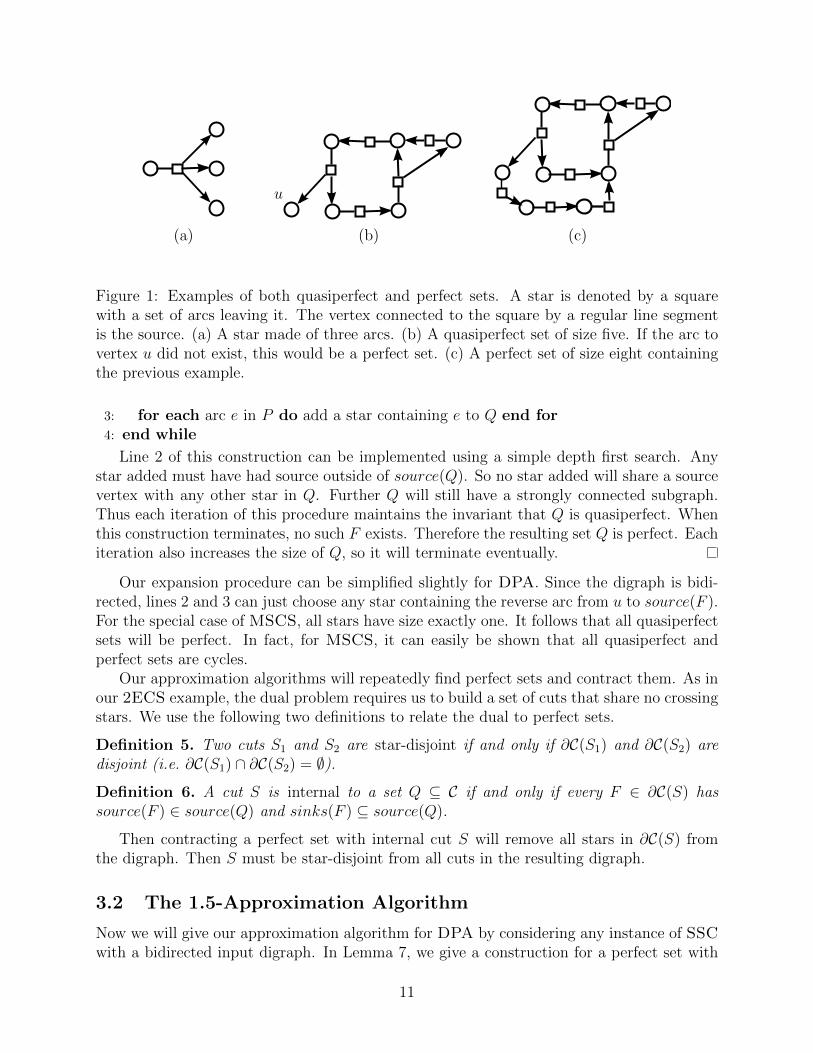
Definition 4. A set Q ⊆ C is perfect if and only if Q is quasiperfect and all F ∈ Q havesinks(F ) ⊆ source(Q).

We define contracting a perfect set as follows: replace all the source vertices of the perfectset with a single supervertex whose arc set is all arcs with exactly one end point in our perfectset. We can combine duplicate arcs into a single arc during this contraction process. As aresult of contraction, the size of a star may decrease, and a star may be removed if it has noremaining arcs. A quasiperfect Q adds |Q| cost and contracts the |Q| vertices of source(Q)into one, but may have extra arcs leaving the new supervertex. A perfect set has no sucharcs, so the problem after contracting such a set will be another instance of SSC. Our nextlemma describes how to expand any quasiperfect set into a perfect set. This an extension ofLemma 2 given by Calinescu in [3].

Lemma 6. Every quasiperfect set is a subset of some perfect set.

Proof. Consider the following expansion procedure for any quasiperfect set Q.

1: while ∃F ∈ Q with u ∈ sinks(F ) \ source(Q) do2: Find a path P from u to source(Q) that is internally disjoint from Q

10

(a) (b)

u

(c)

Figure 1: Examples of both quasiperfect and perfect sets. A star is denoted by a squarewith a set of arcs leaving it. The vertex connected to the square by a regular line segmentis the source. (a) A star made of three arcs. (b) A quasiperfect set of size five. If the arc tovertex u did not exist, this would be a perfect set. (c) A perfect set of size eight containingthe previous example.

3: for each arc e in P do add a star containing e to Q end for4: end while

Line 2 of this construction can be implemented using a simple depth first search. Anystar added must have had source outside of source(Q). So no star added will share a sourcevertex with any other star in Q. Further Q will still have a strongly connected subgraph.Thus each iteration of this procedure maintains the invariant that Q is quasiperfect. Whenthis construction terminates, no such F exists. Therefore the resulting set Q is perfect. Eachiteration also increases the size of Q, so it will terminate eventually.

Our expansion procedure can be simplified slightly for DPA. Since the digraph is bidi-rected, lines 2 and 3 can just choose any star containing the reverse arc from u to source(F ).For the special case of MSCS, all stars have size exactly one. It follows that all quasiperfectsets will be perfect. In fact, for MSCS, it can easily be shown that all quasiperfect andperfect sets are cycles.

Our approximation algorithms will repeatedly find perfect sets and contract them. As inour 2ECS example, the dual problem requires us to build a set of cuts that share no crossingstars. We use the following two definitions to relate the dual to perfect sets.

Definition 5. Two cuts S1 and S2 are star-disjoint if and only if ∂C(S1) and ∂C(S2) aredisjoint (i.e. ∂C(S1) ∩ ∂C(S2) = ∅).

Definition 6. A cut S is internal to a set Q ⊆ C if and only if every F ∈ ∂C(S) hassource(F ) ∈ source(Q) and sinks(F ) ⊆ source(Q).

Then contracting a perfect set with internal cut S will remove all stars in ∂C(S) fromthe digraph. Then S must be star-disjoint from all cuts in the resulting digraph.

3.2 The 1.5-Approximation Algorithm

Now we will give our approximation algorithm for DPA by considering any instance of SSCwith a bidirected input digraph. In Lemma 7, we give a construction for a perfect set with

11

two star-disjoint internal cuts. Utilizing this lemma, our approximation algorithm becomesvery simple. Our algorithm will repeatedly apply this construction and contract the resultingperfect set. This procedure is formally given in Algorithm 2.

Algorithm 2 Dual-Based Approximation for Dual Power Assignment

1: R = ∅2: while |V | 6= 1 do3: Find a perfect set Q with two star-disjoint internal cuts as shown in Lemma 74: Contract the sources of Q into a single vertex5: R := R ∪Q6: end while

Lemma 7. Every instance of SSC with a bidirected input digraph has a perfect set with twostar-disjoint internal cuts.

Proof. We consider an instance of SSC defined on a bidirected digraph G = (V,E). In thedegenerate case, we have a digraph with only two vertices, u and v. Then the perfect set{{uv}, {vu}} will have star-disjoint internal cuts {u} and {v}.

Now we assume |V | ≥ 3. Again, we let N(v) denote the neighbors of a vertex v. Notethat the set of in-neighbors and out-neighbors for a vertex are identical since the digraph isbidirected. We call any vertex with exactly one neighbor a leaf. Then our assumption that|V | ≥ 3 implies some non-leaf vertex exists. Consider the following cycle construction in G(Figure 2 shows its possible outputs).

1: Set P to be any arc rv ∈ E, where v is not a leaf2: while TRUE do3: if ∃u ∈ V s.t. u ∈ N(v) \ V (P ) and u is not a leaf then4: P := P concatenated with the arc vu5: v := u6: else7: Set w to be the vertex in N(v) ∩ V (P ) earliest in P8: Set w to be the successor of w in P9: if ∃u ∈ V s.t. u ∈ N(w) \ V (P ) and u is not a leaf then10: Replace P with the path using wv instead of ww, reversing all arcs between v

and w11: P := P concatenated with the arc wu12: v := u13: else14: Set x to be the vertex in N(w) ∩ V (P ) earliest in P15: Set C to the cycle using the arc vw, the reverse of arcs in P from w to x, the arc

xw, and arcs in P from w to v16: return C, v, w17: end if18: end if19: end while

12

x

w

w

v v = w

x = w

p

p

(a) (b)

Figure 2: Examples of cycles produced by our construction for Lemma 7. Dashed curvesrepresent a path. We do not show the leaves that may exist next to v or w. (a) Shows thegeneral form of our cycle. (b) Shows the special case when |C| = 2.

Note that it is possible for v and w to be the same vertex. We make the following claimabout the output of this procedure.

Lemma 8. For any instance of SSC with a bidirected input digraph and |V | ≥ 3, this con-struction will output a cycle C with vertices v, w ∈ V (C) having the following two properties:

1. v and w are not leaves.

2. Each neighbor of v or w is either in V (C) or a leaf.

Proof. Any strongly connected digraph with at least three vertices will have an initial arcrv where v is not a leaf. This guarantees that step 1 is possible. Then each iterationincreases the length of the path P . It follows that there are at most |V | iterations before theconstruction terminates.

For our first property, we maintain the invariant that v is not a leaf. This is true fromour initial choice of v, and also maintained in each u ∈ V chosen to extend P . Finally, w iseither equal to v and thus not a leaf, or inside the path P and thus has two neighbors.

For our second property, the choice of the cycle C implies that V (C) contains all verticesin P between x and v. All non-leaf neighbors of w are at most as early as x in P . Allnon-leaf neighbors of v are at most as early as w in P . Note that w is at most as early as xin p. Then all the non-leaf neighbors of v and w must be in the V(C).

Using this cycle C, we will construct our perfect set with two star-disjoint internal cuts.Note our resulting perfect set may not fully contain C. Let Lv and Lw be the set of leavesadjacent to v and w, respectively. Consider the case where there is a star F sourced at vcontaining arcs to multiple leaves. Let l1 and l2 be two distinct leaves in sinks(F ). Thenwe expand the quasiperfect set {F} into a perfect set Q using Lemma 6. The resulting setis shown in Figure 3 (a). This Q will have internal cuts {l1} and {l2}. Note that if two cutsshare no vertices, then they also share no crossing stars (i.e. they are star-disjoint). Thesame construction can be made for such a star sourced at w. For the remainder of our proof,we can assume no star exists sourced from v or w going to multiple leaves. Now we considertwo separate cases: v = w and v 6= w.

13

v

l1 l2

(a) (b)

v = w

x = w

p

l

v = w

x = w

p

l

(c)

v

u

l

(d)

v

w

(e)

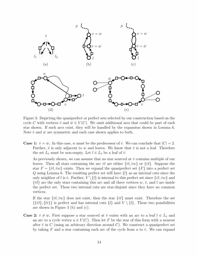
Figure 3: Depicting the quasiperfect or perfect sets selected by our construction based on thecycle C with vertices v and w ∈ V (C). We omit additional arcs that could be part of eachstar shown. If such arcs exist, they will be handled by the expansion shown in Lemma 6.Note v and w are symmetric and each case shown applies to both.

Case 1: v = w. In this case, w must be the predecessor of v. We can conclude that |C| = 2.Further, v is only adjacent to w and leaves. We know that v is not a leaf. Thereforethe set Lv must be non-empty. Let l ∈ Lv be a leaf of v.

As previously shown, we can assume that no star sourced at v contains multiple of ourleaves. Then all stars containing the arc vl are either {vl, vw} or {vl}. Suppose thestar F = {vl, vw} exists. Then we expand the quasiperfect set {F} into a perfect setQ using Lemma 6. The resulting perfect set will have {l} as an internal cuts since theonly neighbor of l is v. Further, V \{l} is internal to this perfect set since {vl, vw} and{vl} are the only stars containing this arc and all three vertices w, v, and l are insidethe perfect set. These two internal cuts are star-disjoint since they have no commonvertices.

If the star {vl, vw} does not exist, then the star {vl} must exist. Therefore the set{{vl}, {lv}} is perfect and has internal cuts {l} and V \ {l}. These two possibilitiesare shown in Figure 3 (b) and (c).

Case 2: v 6= w. First suppose a star sourced at v exists with an arc to a leaf l ∈ Lv andan arc to a cycle vertex u ∈ V (C). Then let F be the star of this form with u nearestafter v in C (using an arbitrary direction around C). We construct a quasiperfect setby taking F and a star containing each arc of the cycle from u to v. We can expand

14

this quasiperfect set into a perfect set Q using Lemma 6. Then {l} is an internal cutto Q. This perfect set is shown in Figure 3 (d). We know that any star F sourced atv with an arc to l cannot have an arc to any other leaf. Then our choice of Q gives usthat all stars F crossing the cut V \ {l} have sinks(F ) ⊂ source(Q). Therefore thecut V \ {l} is also internal to Q.

Now, we can assume no star sourced at v exists with arcs into both Lv and V (C). Thenevery star F crossing the cut {v} ∪ Lv has sinks(F ) ⊂ V (C). The same claim holdsfor w by symmetry. Then we construct a quasiperfect set by iterating over the arcs ofC, selecting a star containing each arc. Let Q be the perfect set made by expandingthis quasiperfect set using Lemma 6. This perfect set is shown in Figure 3 (e). We willhave {v} ∪ Lv as an internal cut since V (C) ⊆ source(Q). Similarly we also have theinternal cut {w} ∪ Lw. Since v 6= w, the two internal cuts are star-disjoint.

Therefore in either of our cases we can construct a perfect set with two star-disjointinternal cuts. This concludes our proof of Lemma 7.

3.3 Analysis of 1.5-Approximation Ratio

Let I be the set of all possible SSC problem instances with bidirected input digraphs. Wedenote the solution from our algorithm on some I ∈ I as A(I) and the optimal solution asOPT (I). We let k denote the total number of perfect sets added by our algorithm. Further,we let Ai denote the number of perfect sets of size i added by the algorithm.

Lemma 9. |A(I)| = n+ k − 1

Proof. Observe that Ai = 0 for any i > n since the source of stars in a perfect set aredistinct. Each perfect set of size i contracts i − 1 vertices, and over the whole algorithm,we contract n vertices into 1. Therefore

∑ni=2(i − 1)Ai = n − 1. Each perfect set of size i

contributes i cost to our solution. Then our cost is∑n

i=2 iAi = n+ k − 1.

Lemma 10. |OPT (I)| ≥ n

Proof. Consider the dual solution of assigning one to the cut {v} for all v ∈ V . This dualfeasible solution has objective n. The lemma follows from weak duality.

Lemma 11. |OPT (I)| ≥ 2k

Proof. Whenever the algorithm adds a perfect set, we can identify two star-disjoint internalcuts. We construct a dual feasible solution by assigning each of our internal cuts yS = 1. Toaccomplish this, we must show that no star F crosses multiple of our internal cuts. Considerany star F ∈ C crossed by at least of our cuts. Let S be the first of our internal cuts withF ∈ ∂C(S). Since S is an internal cut, all arcs of F will be removed from the graph aftercontracting the corresponding perfect set. Thus this F will be crossing at most one of ourinternal cuts. So we have a dual feasible solution with objective 2k. The lemma follows fromweak duality.

15

By taking a convex combination of Lemmas 10 and 11, we know the following:

|OPT (I)| ≥ 2

3n+

1

3(2k). (1)

Taking the ratio of Lemma 9 and Equation (1), we get a bound on the approximationratio. Straightforward algebra on this ratio completes our proof of Theorem 1:

|A(I)||OPT (I)|

≤ n+ k − 12n3

+ 2k3

<3

2= 1.5.

As a corollary, 1.5 upper bounds the ratio between integer primal and integer dual solu-tions to our program. This is easily verified on any SSC instance I by choosing A(I) for theinteger primal and the larger of the two dual solutions used in Lemma 10 and 11. Corollary 1follows from this observation. Further, our analysis of the approximation ratio is tight asshown by an example in our appendix.

Theorem 3. The 1.5-approximation ratio of Algorithm 2 is tight.

4 A 1.6-Approximation for SSC

As in our approximation for DPA, we need a method to construct perfect sets with internalcuts. Without the restriction to bidirected input digraphs, we are unable the guaranteetwo star-disjoint internal cuts in each perfect set. Such a construction would give SSC a1.5-approximation. Instead, we guarantee the following weaker condition.

Lemma 12. Every instance of SSC has a perfect set Q with either |Q| ≥ 4 and one internalcut, or two star-disjoint internal cuts.

Proof. We use N+(v) to denote the set of out-neighbors of a vertex v in G. We use thefollowing cycle construction, which is a simplification of the construction used for DPA.

1: Set P to be any arc rv ∈ E2: while ∃u ∈ N+(v) \ V (P ) do3: P := P concatenated with the arc vu4: v := u5: end while6: Set w to be the vertex in N+(v) earliest in P7: Set C to the cycle using vw and arcs in P8: return C and v

Lemma 13. This construction will output a cycle C and v ∈ V (C) such that N+(v) ⊆ V (C).

Proof. Follows immediately from our choice of C.

Using this C and v, we will construct our perfect set. We consider this in three separatecases: |C| ≥ 4, |C| = 3, and |C| = 2.

16

Case 1: |C| ≥ 4. We construct a quasiperfect set by iterating over the arcs of our cycle C,selecting a star containing each arc. Then let Q be the perfect set created by expandingthis set using Lemma 6. Note that |Q| ≥ 4. Since N+(v) ⊂ V (C), the cut {v} will beinternal to Q.

Case 2: |C| = 3. Our cycle construction must have found a cycle C on vertices {v, u1, u2}.Then v has the property that N+(v) ⊆ {u1, u2}. Suppose some of the cycle arcs, vu1,u1u2, or u2v, are part of a star with a vertex outside our cycle in its sink set. Thenwe can construct a quasiperfect set containing this star and a star for each other arcin the cycle. Expanding this quasiperfect set, as defined in Lemma 6, will produce aperfect set of size four or more with the internal cut {v}. So we assume that no suchF exists, and thus C is a perfect set.

If there exists a nontrivial path from u1 to u2 or from u2 to v internally disjoint fromV (C), then we can replace an arc of C with this path to get a larger cycle that hasthe same property with respect to v (nontrivial meaning with |P | ≥ 2). Then we canapply Case 1 to handle the new cycle.

Similarly, we can assume at least one of the following does not exist: path from u2

to u1 internally disjoint from V (C), path from u1 to v internally disjoint from V (C),or the arc from v to u2. If all three of these existed and at least one of the paths isnontrivial, we could construct a larger cycle with the same property with respect to vby starting at v, following the arc to u2, following the path to u1, finally following thepath to v. We know the paths from u2 to u1 and u1 to v are internally disjoint becauseany overlap would create a path from u2 to v. Thus this construction will produce alarger cycle containing all of neighbors of v. Then we can assume this structure doesnot exist.

We handle the four possible cases of our assumption separately. Note that the strongconnectivity of the digraph implies there exists a path between any pair of vertices. LetRC(u) be the set of vertices reachable by u without using any arcs with both endpointsin C.

Subcase 2.1 No path from u2 to u1 exists that is internally disjoint from V (C). Notethat we also assume no nontrivial path from u2 to v exists. Then RC(u2) includesneither v nor u1. Further, the only arc crossing RC(u2) is u2v (since we haveassumed the arc u2u1 does not exist). It follows that RC(u2) is internal to anyperfect set contracting all three cycle vertices since no star contains a cycle arcand an arc to a fourth external vertex.

Furthermore, the cut {v} will be internal to any perfect set contracting all threecycle vertices. Therefore we select any star containing each of our cycle arcs toproduce a perfect set with internal cuts {v} and RC(u2). These two cuts arestar-disjoint since they have no vertices in common.

Subcase 2.2 No path from u1 to v exists that is internally disjoint from V (C). Notethat we also assume no nontrivial path from u1 to u2 exists. Then RC(u1) includesneither v nor u2. Further, the only arc crossing this cut is u1u2 (since we have

17

assumed the arc u1v does not exist). It follows that RC(u1) is internal to anyperfect set contracting all three cycle vertices since no star contains a cycle arcand an arc to a fourth external vertex.

Furthermore, the cut {v} will be internal to any perfect set contracting all threecycle vertices. Therefore we select any star containing each of our cycle arcs toproduce a perfect set with internal cuts {v} and RC(u1). These two cuts arestar-disjoint since they have no vertices in common.

Subcase 2.3 The arc vu2 does not exist. Again, we select a perfect set made byselecting a star containing each arc of our cycle. The cut {v} is internal to Cfrom our choice of C and v. Further, we know that no nontrivial path existsfrom v to u2 internally disjoint from V (C) and no nontrivial path exists from u1

to u2. Then we can conclude that the cut {v} ∪ RC(u1) is only crossed by thearc u1u2 (since vu2 does not exist). Since we assumed no star containing a cyclearc and an arc to a fourth external vertex exists, {v} ∪RC(u1) is also internal toour perfect set. These two cuts are star-disjoint because the arc vu2 does not exist.

Subcase 2.4 The arcs vu2, u2u1 and u1v exist, but no nontrivial paths exist from u2

to u1 or from u1 to v internally disjoint from V (C). Suppose any of the reversedcycle arcs vu2, u2u1 or u1v are part of a star containing an arc to a fourth vertexoutside of V (C). Then we could construct a perfect set of size four or more withinternal cut {v} based on this cycle.

Now we assume no such stars exist. We select our perfect set by choosing anystar containing each of our cycle arcs. The cut {v} will be internal to such aperfect set. Since no nontrivial path exists from u1 to u2 or to v that is internallystar-disjoint from V (C), the cut RC(u1) will only be crossed by the arcs u1u2 andu1v. Thus RC(u1) is internal to our perfect set. These two cuts are star-disjointsince they have no vertices in common.

Thus under any case we can find two star-disjoint internal cuts in our cycle or a largerperfect set with one internal cut.

Case 3: |C| = 2. Our cycle construction must have found a cycle C on vertices {v, u1}.Note that the only arc leaving v goes to u1, and there is a star containing only thisarc. The strong connectivity of our digraph implies there is a path from u1 to v. If anontrivial path Q exists from u1 to v, then we can replace C with the cycle made byconcatenating the arc vu1 with Q. This larger cycle can then be processed by eitherCase 1 or 2. So we can assume that the only path from u1 to v is the arc between them.Consider the cut V \ {v}, which is only crossed by u1v. Either there exists a F1 ∈ Ccontaining u1v and some u1u2, or this cut is internal to any perfect set contracting vand u1. In the latter case, we can choose the perfect set {{vu1}, {u1v}}. This perfectset has two star-disjoint internal cuts: {v} and V \ {v}.If this F1 and u2 exist, then any nontrivial path Q from u2 to u1 would create aquasiperfect set of size at least four. Then by Lemma 6, we could find a perfect set of

18

size four or more with the internal cut {v}. Finally, we handle the case where the onlypath from u2 to u1 is the arc u2u1. Let R ⊂ V be the set of all vertices that can bereached by u2 without using the arc u2u1. Consider the cut given by R, which is onlycrossed by u2u1. Either there exists a F2 ∈ C containing u2u1 and some u2u3, or R isinternal to any perfect set contracting u1 and u2. In the former case, expanding thequasiperfect set {F1, F2}, as defined in Lemma 6, will give a perfect set of size at leastfour with internal cut {v}. In the latter case, expanding the quasiperfect set {F1}, asdefined in Lemma 6, will give a perfect set with two star-disjoint internal cuts: {v}and R.

Therefore regardless of the size of C, we can construct either a size four or more perfectset with an internal cut or a smaller perfect set with two star-disjoint internal cuts. Thisconcludes our proof of Lemma 12.

Using Lemma 12, our approximation algorithm is very simple. We repeatedly applythis construction and contract the resulting perfect set. This procedure is formally given inAlgorithm 3.

Algorithm 3 Dual-Based Approximation for Star Strong Connectivity

1: R = ∅2: while |V | 6= 1 do3: Find a perfect set Q as shown in Lemma 124: Contract the sources of Q into a single vertex5: R := R ∪Q6: end while

4.1 Analysis of 1.6-Approximation Ratio

The analysis of our approximation ratio is very similar to the analysis given in Section 3.3.Let I be the set of all possible SSC problem instances. We denote the solution from ouralgorithm on some I ∈ I as A(I) and the optimal solution as OPT (I). We let Ai denotethe number of perfect sets of size i added by the algorithm.

Lemma 14. |A(I)| =n∑

i=2

iAi

Proof. Each perfect set in Ai has i stars, and thus contributes i cost to our solution.

Lemma 15. |OPT (I)| ≥ n >n∑

i=2

(i− 1)Ai

Proof. Consider the dual solution of assigning one to the cut {v} for all v ∈ V . This dualfeasible solution has objective n. Since each perfect set of size i added by the algorithm

contracts i − 1 vertices, we know that n − 1 =n∑

i=2

(i − 1)Ai. The lemma follows from weak

duality.

19

Lemma 16. |OPT (I)| ≥ 2A2 + 2A3 +n∑

i=4

Ai

Proof. Whenever the algorithm adds a perfect set of size two, we can identify two star-disjoint internal cuts. Similarly, there are two star-disjoint internal cuts in every perfectset of size three and one internal cut in the remaining perfect sets. From the definition ofinternal cuts, we know that all of these internal cuts will be star-disjoint from previouslyadded internal cuts. So we have a dual feasible solution and the lemma follows from weakduality.

By taking a convex combination of Lemmas 15 and 16, we know the following:

|OPT (I)| > 3

4(

n∑i=2

(i− 1)Ai) +1

4(2A2 + 2A3 +

n∑i=4

Ai)

=5

4A2 + 2A3 +

n∑i=4

(3

4i− 1

2)Ai. (2)

Taking the ratio of Lemma 14 and Equation (2), we get a bound on the approximationratio. Straightforward algebra on this ratio can show it is at most 8/5:

|A(I)||OPT (I)|

<

n∑i=2

iAi

54A2 + 2A3 +

n∑i=4

(34i− 1

2)Ai

≤ 8

5= 1.6.

This finishes the proof of Theorem 2. Corollary 2 follows from the same observation madeabout our 1.5-approximation for DPA. Further, our analysis of the approximation ratio istight as shown by an example in our appendix.

Theorem 4. The 1.6-approximation ratio of Algorithm 3 is tight.

5 Conclusion

We introduced a novel approach to approximating network design problems with cut-basedlinear programming relaxations. Our method combines the combinatorial (recursive) struc-ture of the problem with the cut-based structure produced by the corresponding dual linearprogram. Identifying subgraphs that meet both the recursive and dual structural constraintscan produce provably good approximations.

We applied this methodology to a number of standard network design problems. In thecase of Minimum 2-Edge-Connected Spanning Subgraph, the resulting algorithm isequivalent to a previously proposed 3/2-approximation [18]. For the problem of MinimumStrongly Connected Spanning Subgraph, we produce a tight 1.6-approximation.Although this is slightly worse than the 1.5-approximation of Vetta [24], our algorithm hasnotably fewer cases than Vetta’s algorithm.

20

We also applied our dual-based approach to a common power assignment network designproblem. The resulting algorithm for Dual Power Assignment achieves the best approx-imation ratio known of 1.5 (improving on the previous best known 1.57-approximation of [1]).We introduced a new problem generalizing DPA and MSCS, which we call Star StrongConnectivity. Our approach gives a tight 1.6-approximation to SSC. Each of our ap-proximation results also proves an upper bound on the integrality gap of the correspondingproblem.

Our dual-based approach can likely be applied to other unweighted connectivity problemswith cut-based linear programs. Further application of this method will likely produce newapproximation algorithms and improved upper bounds on their integrality gaps. Anotherinteresting extension of this work would generalize SSC to have costs on each star. Evenwhen costs are constrained to be in {0, 1}, Weighted SSC is at least as hard to approx-imate as Set Cover. This follows from a very simple reduction that was observed in [3].As a consequence, any work on approximating the weighted variant will at best achieve alogarithmic approximation ratio. We believe the methods used in [4] will generalize to giveWeighted SSC such a logarithmic approximation.

Acknowledgments. This research was supported in part by a College of Science Under-graduate Summer Research Award at the Illinois Institute of Technology. We thank GruiaCalinescu for his many valuable comments and fruitful discussions, which notably improvedthe paper.

References

[1] Karim Abu-Affash, Paz Carmi, and Anat Parush Tzur. Dual power assignment viasecond Hamiltonian cycle. arXiv preprint, arXiv:1402.5783, 2014.

[2] Gruia Calinescu. Approximate min-power strong connectivity. SIAM J. Discrete Math.,27(3):1527–1543, 2013.

[3] Gruia Calinescu. 1.61-approximation for min-power strong connectivity with two powerlevels. Journal of Combinatorial Optimization, pages 1–21, 2014.

[4] Gruia Calinescu, Sanjiv Kapoor, Alexander Olshevsky, and Alexander Zelikovsky. Net-work lifetime and power assignment in ad hoc wireless networks. In Giuseppe Di Bat-tista and Uri Zwick, editors, Algorithms - ESA 2003, volume 2832 of Lecture Notes inComputer Science, pages 114–126. Springer Berlin Heidelberg, 2003.

[5] Gruia Calinescu and Kan Qiao. Asymmetric topology control: Exact solutions and fastapproximations. In INFOCOM, 2012 Proceedings IEEE, pages 783–791, March 2012.

[6] Paz Carmi and Matthew J. Katz. Power assignment in radio networks with two powerlevels. Algorithmica, 47(2):183–201, 2007.

21

[7] Jian-Jia Chen, Hsueh-I Lu, Tei-Wei Kuo, Chuan-Yue Yan, and Ai-Chun Pang. Dualpower assignment for network connectivity in wireless sensor networks. In GlobalTelecommunications Conference, 2005. GLOBECOM ’05. IEEE, volume 6, pages 5 pp.–3642, Dec 2005.

[8] Wen-Tsuen Chen and Nen-Fu Huang. The strongly connecting problem on multihoppacket radio networks. Communications, IEEE Transactions on, 37(3):293–295, Mar1989.

[9] Harold N. Gabow, Michel X. Goemans, Eva Tardos, and David P. Williamson. Ap-proximating the smallest k-edge connected spanning subgraph by LP-rounding. Netw.,53(4):345–357, July 2009.

[10] Michael R. Garey and David S. Johnson. Computers and Intractability: A Guide to theTheory of NP-Completeness. W. H. Freeman & Co., New York, NY, USA, 1979.

[11] Benjamin Grimmer and Kan Qiao. Near linear time 5/3-approximation algorithms fortwo-level power assignment problems. In Proceedings of the 10th ACM InternationalWorkshop on Foundations of Mobile Computing, FOMC ’14, pages 29–38, New York,NY, USA, 2014. ACM.

[12] Anupam Gupta and Jochen Koenemann. Approximation algorithms for network design:A survey. Surveys in Operations Research and Management Science, 16(1):3 – 20, 2011.

[13] Mohammadtaghi Hajiaghayi, Nicole Immorlica, and Vahab S. Mirrokni. Power opti-mization in fault-tolerant topology control algorithms for wireless multi-hop networks.In in Proceedings of the 9th Annual International Conference on Mobile Computing andNetworking. 2003, pages 300–312. ACM Press, 2003.

[14] Kamal Jain. A factor 2 approximation algorithm for the generalized steiner networkproblem. Combinatorica, 21(1):39–60, 2001.

[15] Raja Jothi, Balaji Raghavachari, and Subramanian Varadarajan. A 5/4-approximationalgorithm for minimum 2-edge-connectivity. In Proceedings of the Fourteenth AnnualACM-SIAM Symposium on Discrete Algorithms, SODA ’03, pages 725–734, Philadel-phia, PA, USA, 2003. Society for Industrial and Applied Mathematics.

[16] Samir Khuller, Balaji Raghavachari, and Neal Young. Approximating the minimumequivalent digraph. SIAM Journal on Computing, 24(4):859–872, 1995.

[17] Samir Khuller, Balaji Raghavachari, and Neal Young. On strongly connected digraphswith bounded cycle length. Discrete Applied Mathematics, 69(3):281 – 289, 1996.

[18] Samir Khuller and Uzi Vishkin. Biconnectivity approximations and graph carvings. J.ACM, 41(2):214–235, March 1994.

[19] Bundit Laekhanukit, Shayan Oveis Gharan, and Mohit Singh. A rounding by samplingapproach to the minimum size k-arc connected subgraph problem. In Proceedings of the39th International Colloquium Conference on Automata, Languages, and Programming- Volume Part I, ICALP’12, pages 606–616, Berlin, Heidelberg, 2012. Springer-Verlag.

22

[20] Nhat X. Lam, Trac N. Nguyen, Min Kyung An, and Dung T. Huynh. Dual power assign-ment optimization and fault tolerance in wsns. Journal of Combinatorial Optimization,30(1):120–138, 2015.

[21] Tobias Polzin and Siavash Vahdati Daneshmand. On Steiner trees and minimum span-ning trees in hypergraphs. Oper. Res. Lett., 31(1):12–20, 2003.

[22] Ram Ramanathan and Regina Rosales-Hain. Topology control of multihop wirelessnetworks using transmit power adjustment. In INFOCOM 2000. Nineteenth AnnualJoint Conference of the IEEE Computer and Communications Societies. Proceedings.IEEE, volume 2, pages 404–413 vol.2, 2000.

[23] Santosh Vempala and Adrian Vetta. Factor 4/3 approximations for minimum 2-connected subgraphs. In Klaus Jansen and Samir Khuller, editors, Approximation Al-gorithms for Combinatorial Optimization, volume 1913 of Lecture Notes in ComputerScience, pages 262–273. Springer Berlin Heidelberg, 2000.

[24] Adrian Vetta. Approximating the minimum strongly connected subgraph via a match-ing lower bound. In Proceedings of the Twelfth Annual ACM-SIAM Symposium onDiscrete Algorithms, SODA ’01, pages 417–426, Philadelphia, PA, USA, 2001. Societyfor Industrial and Applied Mathematics.

[25] Chen Wang, Myung-Ah Park, James Willson, Yongxi Cheng, Andras Farago, and WeiliWu. On approximate optimal dual power assignment for biconnectivity and edge-biconnectivity. Theoretical Computer Science, 396(13):180 – 190, 2008.

[26] Roger Wattenhofer., Li Li, Paramvir Bahl, and Yi-Min Wang. Distributed topologycontrol for power efficient operation in multihop wireless ad hoc networks. In INFOCOM2001. Twentieth Annual Joint Conference of the IEEE Computer and CommunicationsSocieties. Proceedings. IEEE, volume 3, pages 1388–1397 vol.3, 2001.

[27] Liang Zhao, Hiroshi Nagamochi, and Toshihide Ibaraki. A linear time 5/3-approximation for the minimum strongly-connected spanning subgraph problem. Inf.Process. Lett., 86(2):63–70, April 2003.

A Proof of Lemma 5

Consider some instance of SSC given by a digraph G = (V,E) and a set of stars C. LetROPT ⊆ C be the optimal solution to SSC. Let x∗ be the optimal solution to SSC PrimalLP when restricted to xF ∈ Z. We then need to show that |ROPT | =

∑F∈C x

∗F .

First we show that |ROPT | ≥∑

F∈C x∗F . Consider the vector x produced by assigning all

F ∈ ROPT value 1 and the rest value 0. Then |ROPT | =∑

F∈C xF . Our inequality will followif we show x is a feasible solution to SSC Primal LP, since x∗ is the minimum feasiblesolution. From our construction, all xF ≥ 0. Further consider any cut ∅ ⊂ S ⊂ V . SinceROPT produces a strongly connected spanning subgraph, some F ∈ ROPT crosses S. Sincethis xF = 1, we know

∑F∈∂C(S) xF ≥ 1. Thus x is feasible.

23

v w

u1 u2 u3uk

uk+1

l1 l2 l3 lk...

...

Figure 4: Example instance of Gk used to show our 1.5-approximation ratio for DPA istight.

Now we prove that |ROPT | ≤∑

F∈C x∗F . We know that all x∗F ∈ {0, 1} (if a larger

x∗F exists, our objective is reduced by reducing it to x∗F = 1 without effecting feasibility).Consider the set of stars R = {F |x∗F = 1}. Then |R| =

∑F∈C x

∗F . Our inequality will follow

if we show R is a feasible solution to SSC, since ROPT is the minimum feasible solution. Weprove this by contradiction. Let G′ be the digraph induced by R (i.e. G′ = (V,

⋃F∈R F )).

Assume G′ is not strongly connected. Then there exists s, t ∈ V such that there is no s, t-path in G′. Consider the set Vs ⊆ V of all vertices u with a s, u-path. Note t /∈ Vs. ThenVs is a cut with no arcs or stars crossing it. However, this contradicts the fact that x∗ isfeasible. Thus we can conclude R is feasible. Lemma 5 follows.

B Tightness of 1.5-Approximation Ratio for DPA

We prove this by giving a family Gk of instances of SSC with a bidirected input digraphswhere our algorithm can choose arbitrarily close to 3|OPT (Gk)|/2 stars. Our family ofinstances will only have stars of size one. Therefore, we can represent an instance of SSCusing only the corresponding digraph. Further, since the digraph must be bidirected, we canrepresent it using an undirected graph.

We define our family Gk as follows: Let V (Gk) = {v, w} ∪ {u1, u2, ...uk+1} ∪ {l1, l2, ...lk}.Let E(Gk) contains vuk+1, wuk, and all edges in the cycle v, u1, u2, ...uk+1w and the cyclev, u1, l1, u2, l2, ...lk, uk+1, w. An example instance of Gk is depicted in Figure 4

Suppose Algorithm 2 is run on Gk. When our cycle construction is run, it could buildthe path uk+1, w, uk, ...u2, u1, v before terminating. Then it would choose the perfect setcorresponding to the cycle v, uk+1, w, uk, ...u2, u1. This set has disjoint internal cuts {v} and{w}. After this is contracted into a vertex s, the algorithm will have to choose the perfectset of size two contracting li into s for each 1 ≤ i ≤ k. Each of these sets have disjointinternal cuts {li} and V \ {li}. Therefore our algorithm could choose 3k + 3 stars.

The optimal solution to Gk will choose the perfect set corresponding to the Hamiltoniancycle v, u1, l1, u2, l2, ...lk, uk+1, w. This solution has objective 2k+3. Then the approximationratio achieved on Gk could be as large as 3k+3

2k+3. As k approaches infinity, the ratio achieved

on Gk approaches 3/2.

24

a

b

c

d

x y

z

a′b′

c′

d′

x′ y′

a′b′

c′

d′

x′ y′

(a) (b)

(c)

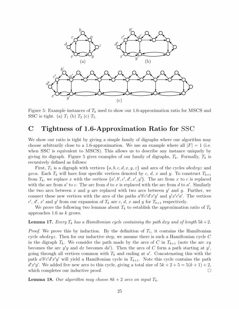
Figure 5: Example instances of Tk used to show our 1.6-approximation ratio for MSCS andSSC is tight. (a) T1 (b) T2 (c) T5

C Tightness of 1.6-Approximation Ratio for SSC

We show our ratio is tight by giving a simple family of digraphs where our algorithm maychoose arbitrarily close to a 1.6-approximation. We use an example where all |F | = 1 (i.e.when SSC is equivalent to MSCS). This allows us to describe any instance uniquely bygiving its digraph. Figure 5 gives examples of our family of digraphs, Tk. Formally, Tk isrecursively defined as follows:

First, T1 is a digraph with vertices {a, b, c, d, x, y, z} and arcs of the cycles abcdxyz andyxca. Each Tk will have four specific vertices denoted by c, d, x and y. To construct Tk+1

from Tk, we replace x with the vertices {a′, b′, c′, d′, x′, y′}. The arc from x to c is replacedwith the arc from a′ to c. The arc from d to x is replaced with the arc from d to a′. Similarlythe two arcs between x and y are replaced with two arcs between y′ and y. Further, weconnect these new vertices with the arcs of the paths a′b′c′d′x′y′ and y′x′c′a′. The verticesc′, d′, x′ and y′ from our expansion of Tk are c, d, x and y for Tk+1 respectively.

We prove the following two lemmas about Tk to establish the approximation ratio of Tkapproaches 1.6 as k grows.

Lemma 17. Every Tk has a Hamiltonian cycle containing the path dxy and of length 5k+2.

Proof. We prove this by induction. By the definition of T1, it contains the Hamiltoniancycle abcdxyz. Then for our inductive step, we assume there is such a Hamiltonian cycle Cin the digraph Tk. We consider the path made by the arcs of C in Tk+1 (note the arc xybecomes the arc y′y and dx becomes da′). Then the arcs of C form a path starting at y′,going through all vertices common with Tk and ending at a′. Concatenating this with thepath a′b′c′d′x′y′ will yield a Hamiltonian cycle in Tk+1. Note this cycle contains the pathd′x′y′. We added five new arcs to this cycle, giving a total size of 5k + 2 + 5 = 5(k + 1) + 2,which completes our inductive proof.

Lemma 18. Our algorithm may choose 8k + 2 arcs on input Tk.

25

Proof. We prove this by induction. For T1, our cycle construction could build the path cayx.Then the cycle cayx with internal cut {x} may be used to create our perfect set. Let w bethe resulting supervertex after contracting these four vertices. The next three iterations ofour algorithm will contract the cycles wd, wb and wz. Total this choose 10 arcs, confirmingour base case.

Now we assume our algorithm will produce a solution to Tk using 8k + 2 arcs. Given aninstance of Tk+1, consider the vertices added in our recursive construction: {a′, b′, c′, d′, x′, y′}.As in our base case, the algorithm may contract the cycle y′x′c′a′ into a supervertex w. Thenit can contract the cycles wd′ and wb′. After these contractions, the six vertices that replacedx in Tk have been combined to a single vertex. Then it follows that after our algorithm selectsthese 8 arcs and contracts, Tk+1 becomes an instance of Tk. By our inductive assumption,this process could choose 8 + (8k + 2) = 8(k + 1) + 2 arcs.

From Lemma 17, we know that the optimal solution to Tk costs 5k + 2. Combiningthis result with Lemma 18, we find Tk could have an approximation ratio of 8k+2

5k+2, which

approaches 8/5 = 1.6.

26