Dual-Polarization Radar Principles and System Operations

Version: 1109

Dual-Polarization Radar Principles

and System Operations

Presented by theWarning Decision Training Branch

CC HCA DPR

Version: 1109

Version: 1109

Table of Contents

Dual-Polarization Radar Principles . . . . . . . . . . . . . . . . . . . . . . . . . . . . 5What Dual-Pol Does Not Change . . . . . . . . . . . . . . . . . . . . . . . . . . . . . . . . . . . . . . . . . . 5Moments vs. Variables . . . . . . . . . . . . . . . . . . . . . . . . . . . . . . . . . . . . . . . . . . . . . . . . . . 6RDA Signal Processing and the Dual-Pol Variables . . . . . . . . . . . . . . . . . . . . . . . . . . . . 7RDA Generation of Differential Reflectivity . . . . . . . . . . . . . . . . . . . . . . . . . . . . . . . . . . . 8RDA Generation of Correlation Coefficient . . . . . . . . . . . . . . . . . . . . . . . . . . . . . . . . . . . 9Differential Phase (ΦDP) and Specific Differential Phase (KDP) . . . . . . . . . . . . . . . . . 16

Dual-Polarization Radar Principles . . . . . . . . . . . . . . . . . . . . . . . . . . . 23Sensitivity Differences . . . . . . . . . . . . . . . . . . . . . . . . . . . . . . . . . . . . . . . . . . . . . . . . . . 23Radar Sensitivity . . . . . . . . . . . . . . . . . . . . . . . . . . . . . . . . . . . . . . . . . . . . . . . . . . . . . . 24Why the Dual-Pol Upgrade Lowers the WSR-88D Sensitivity . . . . . . . . . . . . . . . . . . . 25Calibration . . . . . . . . . . . . . . . . . . . . . . . . . . . . . . . . . . . . . . . . . . . . . . . . . . . . . . . . . . . 28Attenuation . . . . . . . . . . . . . . . . . . . . . . . . . . . . . . . . . . . . . . . . . . . . . . . . . . . . . . . . . . 31Depolarization . . . . . . . . . . . . . . . . . . . . . . . . . . . . . . . . . . . . . . . . . . . . . . . . . . . . . . . . 32Beam Filling Issues . . . . . . . . . . . . . . . . . . . . . . . . . . . . . . . . . . . . . . . . . . . . . . . . . . . . 34Wet Radomes . . . . . . . . . . . . . . . . . . . . . . . . . . . . . . . . . . . . . . . . . . . . . . . . . . . . . . . . 38ZDR and the Trees . . . . . . . . . . . . . . . . . . . . . . . . . . . . . . . . . . . . . . . . . . . . . . . . . . . . 39

Life Without CMD and the Dual-Pol Preprocessor . . . . . . . . . . . . . . . 41Wideband on RPG HCI . . . . . . . . . . . . . . . . . . . . . . . . . . . . . . . . . . . . . . . . . . . . . . . . . 41Clutter Management Without Clutter Mitigation and Decision (CMD) . . . . . . . . . . . . . . 42Product Resolution . . . . . . . . . . . . . . . . . . . . . . . . . . . . . . . . . . . . . . . . . . . . . . . . . . . . 52The RPG Dual-Pol Preprocessor . . . . . . . . . . . . . . . . . . . . . . . . . . . . . . . . . . . . . . . . . 54

Hydrometeor Classification Algorithm (HCA) and Melting Layer Detection Algorithm (MLDA) . . . . . . . . . . . . . . . . . . . . . . . . . . . . . . . 61

MLDA Adaptable Parameter . . . . . . . . . . . . . . . . . . . . . . . . . . . . . . . . . . . . . . . . . . . . . 68Summary . . . . . . . . . . . . . . . . . . . . . . . . . . . . . . . . . . . . . . . . . . . . . . . . . . . . . . . . . . . . 69Hydrometeor Classification Algorithm (HCA) . . . . . . . . . . . . . . . . . . . . . . . . . . . . . . . . 69Summary . . . . . . . . . . . . . . . . . . . . . . . . . . . . . . . . . . . . . . . . . . . . . . . . . . . . . . . . . . . . 78

Quantitative Precipitation Estimation (QPE) Algorithm . . . . . . . . . . . 79QPE and PPS in the RPG . . . . . . . . . . . . . . . . . . . . . . . . . . . . . . . . . . . . . . . . . . . . . . . 79QPE and PPS Product Data Levels . . . . . . . . . . . . . . . . . . . . . . . . . . . . . . . . . . . . . . . 80Similar: Storm Total Accumulations . . . . . . . . . . . . . . . . . . . . . . . . . . . . . . . . . . . . . . . 81Similar: Exclusion Zones . . . . . . . . . . . . . . . . . . . . . . . . . . . . . . . . . . . . . . . . . . . . . . . . 84Different: One Hour Product . . . . . . . . . . . . . . . . . . . . . . . . . . . . . . . . . . . . . . . . . . . . . 85Different: QPE Input . . . . . . . . . . . . . . . . . . . . . . . . . . . . . . . . . . . . . . . . . . . . . . . . . . . 86

Version: 1109

Different: Pre-product Product . . . . . . . . . . . . . . . . . . . . . . . . . . . . . . . . . . . . . . . . . . . 86Different: Rain Rate Equations . . . . . . . . . . . . . . . . . . . . . . . . . . . . . . . . . . . . . . . . . . . 88QPE and Melting Layer . . . . . . . . . . . . . . . . . . . . . . . . . . . . . . . . . . . . . . . . . . . . . . . . . 90QPE & R(Z,ZDR) . . . . . . . . . . . . . . . . . . . . . . . . . . . . . . . . . . . . . . . . . . . . . . . . . . . . . 90QPE and Bright Band Contamination . . . . . . . . . . . . . . . . . . . . . . . . . . . . . . . . . . . . . . 91QPE and Hail Contamination . . . . . . . . . . . . . . . . . . . . . . . . . . . . . . . . . . . . . . . . . . . . 91QPE and Non-Uniform Beam Filling . . . . . . . . . . . . . . . . . . . . . . . . . . . . . . . . . . . . . . . 92QPE and ZDR Calibration . . . . . . . . . . . . . . . . . . . . . . . . . . . . . . . . . . . . . . . . . . . . . . . 93QPE Strengths . . . . . . . . . . . . . . . . . . . . . . . . . . . . . . . . . . . . . . . . . . . . . . . . . . . . . . . 93QPE Limitations . . . . . . . . . . . . . . . . . . . . . . . . . . . . . . . . . . . . . . . . . . . . . . . . . . . . . . 93Ongoing QPE Research . . . . . . . . . . . . . . . . . . . . . . . . . . . . . . . . . . . . . . . . . . . . . . . . 94

What Dual-Pol Does Not Change 1 - 5

RDA Lesson 1: Dual-Polarization Radar Principles

What Dual-Pol Does Not Change

Though dual-pol is a significant upgrade, it isimportant to remember that many things do notchange. Some of the key hardware components,such as the transmitter, do not change, including:

• Frequency

• Beamwidth

• Range sampling resolution

The structure of the VCPs does not change,including:

• Elevations sampled

• Azimuthal sampling resolution

• Update time

• Number of pulses per radial

All of the pre-dual-pol products will continue to begenerated, though there are slight differenceswhich are presented in RDA Lesson 2.

Dual-pol has many benefits, but it will take a lot oftime to develop expertise. It is important to bringthe dual-pol products into your methodology atyour own pace and in a way that keeps you frombeing overwhelmed.

1 - 6 Moments vs. Variables

How have the dual-pol data been integrated intothe VCPs? For the Split Cut elevations, the dual-pol data are generated from the ContiguousSurveillance (CS) rotation. This takes advantageof a low PRF with a long Rmax, meaning thatmultiple trip echoes are highly unlikely. For theBatch elevations, the dual-pol data are generatedfrom the Doppler pulses, because there are moreof them available per radial. For the elevationsabove Batch, only Contiguous Doppler (CD) modeis used, because range folding is not a concern.Figure 1-1 shows the breakdown for VCP 12.

Moments vs.Variables

Dual-pol base data are sometimes referred to as“Variables”, while reflectivity, velocity, andspectrum width are referred to as “Moments”. Thisis because reflectivity, velocity, and spectrum widthare moments of the Doppler Spectrum, which is adistribution of returned signal power as a functionof the Doppler Velocity (see Fig. 1-2). You mightremember the Doppler Spectrum from previoustraining modules. We’ll need this tool once againfor concepts related to dual-pol.

Figure 1-1. Dual-pol data are generated from Contiguous Surveillance (CS) rotation on the Split Cut elevations, Doppler pulses for Batch elevations, and Contiguous Doppler (CD) mode above Batch cuts.

RDA Signal Processing and the Dual-Pol Variables 1 - 7

If you are interested in the specifics, reflectivity isthe 0th moment, velocity is the 1st moment, andspectrum width is the 2nd central moment.

RDA Signal Processing and the Dual-Pol Variables

In contrast, we refer to the dual-pol base productsas “Variables”. This module presents the basics ofdual-pol base data generation at the RDA signalprocessor, and the products that are then built bythe RPG.

The first two, differential reflectivity (ZDR) andcorrelation coefficient (CC) are generated by theRDA signal processor, then sent to the RPG andgenerated into a base product.

Differential phase (ΦDP), is also generated by theRDA signal processor. It is base data, but not aproduct. The ΦDP values are transmitted to theRPG along with CC and ZDR. The RPG generates

Figure 1-2. Graph showing returned signal power as a function of Doppler Velocity. Reflectivity, velocity and spectrum width are all moments of the Doppler Spectrum.

1 - 8 RDA Generation of Differential Reflectivity

the specific differential phase (KDP) product.There is no ΦDP base product.

RDA Generation ofDifferentialReflectivity

ZDR is defined as the difference between thehorizontal and vertical reflectivities, eachexpressed in units of dB. However, ZH and ZV arenot calculated directly. The equation in Figure 1-3is a definition of ZDR, while ZDR is calculatedfrom the mean returned power from both the Hand V channels.

Base reflectivity, Z, is still calculated from thereturned power in the horizontal channel only.

Using the Probert-Jones radar equation, the Zvalue for each channel is equal to the returnedpower, times the range squared times a constantthat is based on the radar’s calibration (seeFig. 1-4).

The ZDR equation can be written as ZDR = 10log(ZH/ZV). When the Zs are substituted with returnedpower, the radar constants and the range termscancel. Calibration of both channels is veryimportant for an accurate ZDR. The significance ofZDR calibration will be explored in RDA Lesson 2.

Figure 1-3. Equation expressing the definition of differential reflectivity.

Figure 1-4. The significance of calibration to both channels.

RDA Generation of Correlation Coefficient 1 - 9

RDA Generation ofCorrelationCoefficient

Correlation coefficient measures the consistencyof the H and V returned power and phase for eachpulse. This “cross correlation” looks at how thepower and phase of one channel compares to theother channel. If the consistency is high, changeswith one channel are similar to changes with theother.

CC provides information on the quality of the dual-pol base data estimate and (even better for us)implies information on the nature of the scatterers!

This is in some ways similar to the relationshipbetween spectrum width and velocity. Spectrumwidth measures the consistency of the phaseshifts from one pulse to next, which then relates tothe reliability of the associated velocity value.

CC and spectrum width are analogous, but thereare some important differences. Base velocity andspectrum width are both calculated from the Hchannel only. Phase shifts from one pulse to thenext are compared. A series of pulse pair phaseshifts are averaged for the range bin as a vectorsum (see Fig. 1-5).

Figure 1-5. Graphical representation of the averaging of pulse pair phase shifts for base velocity and spectrum width.

1 - 10 RDA Generation of Correlation Coefficient

The greater the variation of these phase shifts, thegreater the spectrum width. In the reflectivityimage on the left in Figure 1-6, the white circle isan area of weak signal close to an intensesupercell. The middle image shows high spectrumwidth due to both the weak signal and theturbulence. A high spectrum width implies a lowconsistency of pulse to pulse phase shifts. It is aninverse relationship. Notice that the velocity fieldon the right is noisy in the same area.

For each pulse, the returned power and phasefrom the H and V channels are compared to oneanother. This is different from the type ofcorrelation that gives us velocity and spectrumwidth, which is from one pulse to the next.

The consistency that CC measures is based onthe angle, ΦDP, between the H and V vectors,which can be determined by vector multiplication(see Fig. 1-7). This “cross correlation” of H and Vis checked for each pulse. The vectormultiplication of H and V results in the "crosscorrelation" vector for each pulse, and ΦDP is theangle from the positive x-axis of this vector.

Figure 1-6. Reflectivity (left), spectrum width (middle), and velocity (right). The white circle highlights an area of weak signal in the vicinity of a supercell resulting in high spectrum width and noisy velocity returns.


ΦDP is important for two of our dual-pol variables.

1. ΦDP for a series of pulses is part of the calcu-lation of CC.

2. ΦDP is base data generated at the RDA andsent to the RPG. Specific Differential Phase, orKDP, is based on it.

Figure 1-7. Horizontal and vertical vectors from three sample pulses.


Since we don’t assign any type of base data withjust one pulse, the cross correlation vectors for aseries of pulses are summed. Shown in Figure1-8, this vector sum (red arrow) is what’s neededfor the remaining two dual-pol variables. ΦDP isthe angle of this vector sum, and it is part of thebase data generated at the RDA for each rangebin.

CC is calculated by taking the length (oramplitude) of this vector and dividing it by theaveraged H and V powers. Though CC isexpressed as a number between 0 and 1, you canthink of it as a fraction of “perfect” consistency ofscatterers. Keep in mind, that CC is never exactlyequal to 0 or 1.

If pure rain is being sampled, there is minimalvariation between the H and V channels, the crosscorrelation vectors line up nicely like in the imageon the left in Figure 1-9, and CC is close to 1. Themore diverse the scatterers, the more variation

Figure 1-8. Vector sum for the given range bin of five sample pulses, which is known as ΦDP.


with the cross correlation vectors, and CC getscloser to 0.

A potentially confusing point about the meaning ofCC vs. spectrum width is that high CC means highconsistency, while a high spectrum width meanslow consistency. Essentially spectrum width hasan inverse relationship with consistency, while CChas a direct one.

Why Does CC Matter?Low CC (<0.70) implies low consistency betweenH and V in the estimate and lot of diversity of thescatterers. In fact, CC <0.70 is so diverse thescatterers are likely to be non-meteorological,such as birds or insects. This distinction betweenbiological and meteorological targets is one of thegreat benefits of dual-pol.

On the other hand, a high CC (>0.97) tells us thatthe dual-pol base data estimate is high inconsistency between H and V. The scatterers arevery uniform in size and shape, such as pure rainor snow.

In the case of mesoscale melting layer detection(no convective cells), the radar beam is sampling alayer with a mixture of liquid and solidhydrometeors, such as rain and melting snow.This mix of scatterers within the melting layer

Figure 1-9. Examples of cross correlation vectors for high CC (left) and low CC (right).


creates low consistency of H to V, which lowersthe CC value (see Fig. 1-10).

In areas of weak signal, CC is often noisy inappearance and the magnitudes can vary. InFigure 1-11, near the radar (yellow box) the CCvalues are generally low, and there are likely to benon-hydrometeors present. At longer range on thefringe areas of the precipitation (white circles), theCC values are noisy with values greater than 1.CC > 1 is an estimation artifact, meaning that theestimate is unreliable at that location. It would bemisleading to truncate these values at 1, so theyare intentionally displayed as > 1.

Figure 1-10. CC image showing a clearly defined melting layer.

Figure 1-11. Reflectivity (left) and CC (right) images showing the effects of weak signal on CC (white circles).


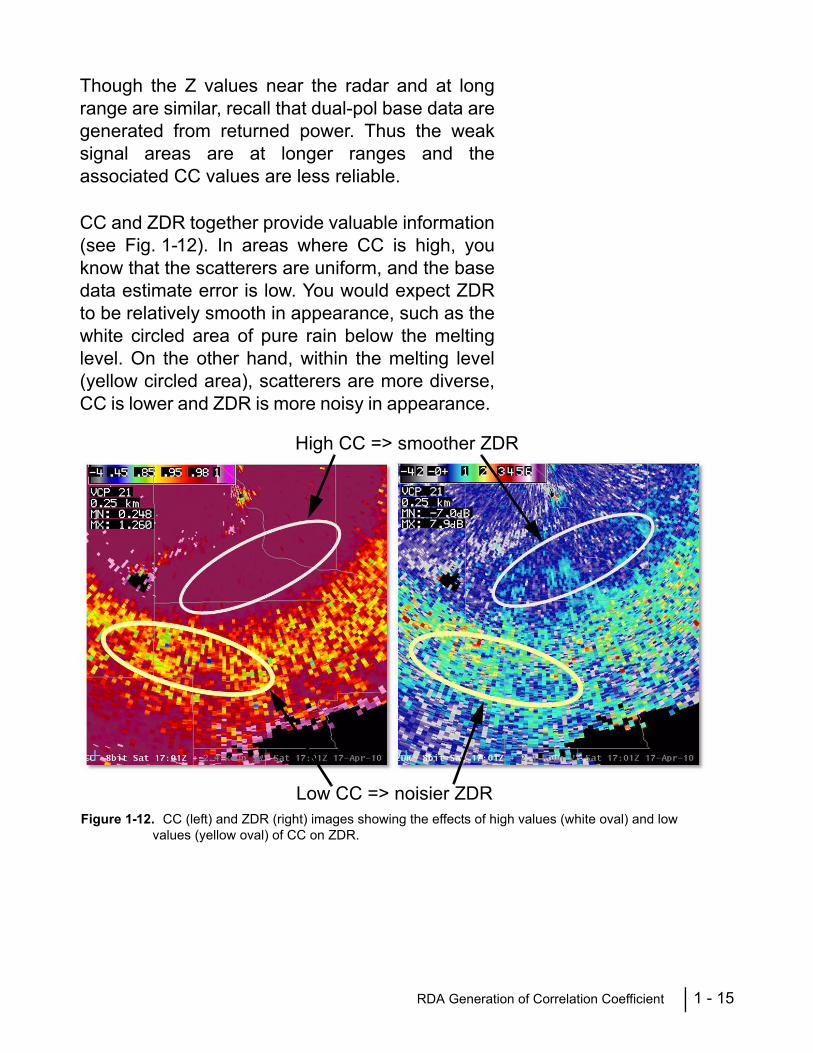
Though the Z values near the radar and at longrange are similar, recall that dual-pol base data aregenerated from returned power. Thus the weaksignal areas are at longer ranges and theassociated CC values are less reliable.

CC and ZDR together provide valuable information(see Fig. 1-12). In areas where CC is high, youknow that the scatterers are uniform, and the basedata estimate error is low. You would expect ZDRto be relatively smooth in appearance, such as thewhite circled area of pure rain below the meltinglevel. On the other hand, within the melting level(yellow circled area), scatterers are more diverse,CC is lower and ZDR is more noisy in appearance.

High CC => smoother ZDR

Low CC => noisier ZDRFigure 1-12. CC (left) and ZDR (right) images showing the effects of high values (white oval) and low

values (yellow oval) of CC on ZDR.

1 - 16 Differential Phase (ΦDP) and Specific Differential Phase (KDP)

Differential Phase(ΦDP) and SpecificDifferential Phase

(KDP)

The third dual-pol base product is specificdifferential phase, or KDP, though it is technically aderived product generated at the RPG. KDP is builtfrom differential phase, or ΦDP, which is generatedby the RDA and sent to the RPG (see Fig. 1-13).Since ΦDP is not available on AWIPS, we think ofKDP as a dual-pol base product.

The benefit of KDP is that it tells you somethingabout the type of medium (light rain? heavy rain?)that the beam has passed through.

In order to understand KDP, we must go back todifferential phase, ΦDP. Recall that for a singlepulse, ΦDP is the angle of the cross correlationvector (see Figure 1-14 on page 1-17).

Figure 1-13. Differential phase (ΦDP) is generated at the RDA and sent to the RPG which then generates specific differential phase (KDP).

Differential Phase (ΦDP) and Specific Differential Phase (KDP) 1 - 17

For a series of pulses, ΦDP is the angle of thevector sum of the cross correlation vectors (seeFig. 1-15).

As the pulse propagates through differentmediums (light rain, heavy rain, etc.), there is adelay that is apparent in the phase of the returnedpulse. Since we have both H and V, we cancompare how the “H delay” differs from the “V

Figure 1-14. ΦDP for a single pulse is the angle of the cross correlation vector.

Single Pulse

Figure 1-15. Vector sum for the given range bin of five sample pulses, which is known as ΦDP (same as Figure 1-8).


delay”. This provides valuable information on thenature of the scatterers that are being sampled.

Liquid water provides “resistance” to the outgoingpulse. In Figure 1-16, the pulse is passing throughraindrops, which have a larger horizontal extentthan vertical. There is more resistance in the Hdirection compared to V, creating a longer delay inthe H phase compared to the V phase. Thereturned phase value for H will be greater than forV and ΦDP >0.

For any given sample volume, the value of ΦDP isaffected by differences in propagation speeds ofthe H and V waves. Propagation is slowed byparticle shape and/or by particle concentration.

Below are two examples that would result in aslower H propagation compared to V, and thus ahigher ΦDP:

1. If the beam is passing through large raindrops,there is more propagation delay in the H direc-tion than in the V direction (see Fig. 1-17, left).

2. Assume the same size and shape raindrops ineach of two sample volumes. However, thereis a greater concentration of them in Figure1-17 on the left. This greater concentration,which means more liquid water content, also

Figure 1-16. Differences in delays from horizontal and vertical channels can provide information about the medium through which the pulse has passed.


creates a greater propagation delay in the Hdirection than in the V direction.

This relationship of ΦDP to liquid water content iswhat makes this dual-pol variable so important!

How ΦDP Changes Along the Radial

Since ΦDP is dependent on propagation, thevalues accumulate down radial. There is no way to“reset” the phase shift as the pulse travelsoutbound, encountering one or more areas ofprecipitation.

In Figure 1-18, the beam first passes through clearair, which leaves the ΦDP values unchanged. Thena rain shaft is encountered, which means ΦDP > 0for a series of range bins, and increases with eachbin in the rain shaft. The beam then progresses to

Figure 1-17. Greater concentration of raindrops leads to greater propogation delay in the H direction than in the V direction.

Figure 1-18. Because ΦDP cannot be reset as the pulse travels outbound, the value is increased with each area of liquid scatterers it encounters.


another patch of clear air and the ΦDP value staysconstant. Finally, another rain shaft isencountered, again increasing the ΦDP valuedown radial. Through this process, the ΦDP valuedoes not “reset” to 0. This makes interpretation ofΦDP as a base product very challenging.

Why KDP? Specific differential phase or KDP is defined as therange derivative of ΦDP, and is the dual-pol baseproduct seen in AWIPS. KDP is a way to capturethe ΦDP changes over very short ranges, whichgives us more useful information. You can think ofit as a “local” variable. Thus the units for KDP aredegrees per km.

The equation in Figure 1-19 does not representthe actual calculation of KDP. It is used torepresent the concept of subtracting ΦDP over arange interval. The actual calculation involves aleast squares fit of multiple differences along theradial, centered at the range bin.

The span of range bins used for the KDPcalculation is dependent on the Z value:

• Z ≥ 40 dBZ

KDP is based on an integration of 9 bins (4bins back and 4 bins forward along theradial)

There is less smoothing required, and fewerbins are used

Figure 1-19. Equation representing the concept of subtracting ΦDP over a range interval.


• Z < 40 dBZ

KDP is based on an integration of 25 bins(12 bins back and 12 bins forward along theradial)

There is the potential for more noise in thedata, thus more bins are used for greatersmoothing

The KDP calculation fits a line to the varying ΦDPvalues along the 9 or 25 bin chunk of the radial.

Figure 1-20 (left) depicts ΦDP values with range fora low diversity of hydrometeors (high CC), such aspure rain or snow. The graphic on the right depictsΦDP values with range for a high diversity ofhydrometeors (low CC), such as mixed rain andsnow. In both cases, KDP is the slope of theselines.

KDP is only calculated for bins with CC > 0.90.The idea is to limit KDP to range bins which arelikely to contain precipitation.

Figure 1-20. KDP is the slope of a line representing ΦDP as a function of range.


KDP and CC From their respective computation methods, KDPand CC are related to one another (see Fig. 1-21).When CC is high, close to 0.99, the hydrometeorsare uniform and both CC and KDP are verysmooth in appearance (white circles). When CCapproaches 0.90, the hydrometeors are mixed insize and shape, and CC and KDP are noisier inappearance, such as in the melting layer (whiteboxes). Also notice that within the melting layerthere are some KDP range gates with no data.This is because the CC values are < 0.90, andKDP is not generated for bins where CC < 0.90.

Figure 1-21. KDP appears smoother with high CC (white circles). For CC values close to 0.90, KDP appears noisy. KDP is not generated for bins where CC < 0.90.

Sensitivity Differences 2 - 23

RDA Lesson 2: Dual-Polarization Radar Principles

Sensitivity Differences

As a result of their design, VCPs 31 and 32 havehad significant sensitivity differences since theinception of the WSR-88D. Visible differences inareal coverage between these VCPs may havebeen noticed without awareness that sensitivity isthe underlying cause. VCP 31 uses long pulse,which means power is transmitted for a longertime. This increases the “power on target” andthus increases the returned power. VCP 31 isabout 4.8 dB more sensitive than VCP 32 (and theother short pulse VCPs). This means that for anygiven range, there may be targets that aredetectable by VCP 31, but not by VCP 32.

Figure 2-1 shows an example of these two VCPsduring a freezing drizzle event. There is morecoverage of this very light precipitation with VCP31 because of its better sensitivity. Thesignificance of sensitivity is also dependent on thetype of weather. The weather events that are mostimpacted by the decrease in sensitivity after thedual-pol upgrade are freezing drizzle and lightsnow.

Figure 2-1. Imagery from a freezing drizzle event showing the differences between long pulse VCP31 (left) and short pulse VCP 32 (right).

VCP 31 VCP 32

2 - 24 Radar Sensitivity

Radar Sensitivity Sensitivity defines the minimum signal that a radarcan detect at a given range. Sensitivity isexpressed as a dBZ value at a given range for areturned signal that is above the system noise by athreshold amount. We’ll call this the powerthreshold.

Transmitted power and system noise are majorcontributors to sensitivity. The more powertransmitted, the more power received, and themore likely we are to have returns above thepower threshold, like the image on the left inFigure 2-2. The greater the system noise, thegreater the power threshold and the less likely thereturned power is sufficiently high. On the right,the system noise is much higher than any radaryou would ever want to use!

The WSR-88D can only “see” targets with returnedpower that exceeds the power threshold.

The combination of transmitted power and systemnoise determines whether or not the returnedsignal of a given target is sufficiently strong forvalid weather data. If the returned signal is belowthe power threshold, it would have too much errorto be acceptable, and the base data are not

Figure 2-2. Only returned power above the power threshold (left) can be used to generate valid base data. If the system noise and power threshold are too high (right), the error is too high and the base data are not sent to the RPG.

Why the Dual-Pol Upgrade Lowers the WSR-88D Sensitivity 2 - 25

transmitted to the RPG. For a given target,sensitivity determines whether or not data areassigned to the relevant gate on a radar product.

For the same system noise, the higher thetransmitted power, the higher the returned power,and the better the sensitivity. The two graphics inFigure 2-3 show a strong signal for single vs. dual-pol, but the dual-pol returned power is lower.

Why the Dual-Pol Upgrade Lowers the WSR-88D Sensitivity

The reduction in sensitivity starts with a basicrequirement of dual-pol: the WSR-88D must beable to transmit and receive waves that arepolarized both horizontally and vertically orientedas shown in Figure 2-4.

Figure 2-3. For a strong signal, the returned power is higher for single polarization (left) than for dual polarization (right).

Figure 2-4. The very definition of dual-pol, it’s horizontal and vertical waves, cause a reduction in sensitivity.

2 - 26 Why the Dual-Pol Upgrade Lowers the WSR-88D Sensitivity

It is important to remember that returned power isnot the same as dBZ, and this will be addressedas part of the discussion on the calibration of Z.

Splitting TransmittedPower Into H and V

Channels

So how to transmit a Horizontal (H) and Vertical(V) signal without buying an extra transmitter? Thesolution is to split the transmitted pulse into the Hand V channels, then send them to the antenna.Upon return, the H and V channel pulses areanalyzed separately (see Fig. 2-5).

Splitting the transmitted power, with one half goinginto each channel results in a 3 dB loss intransmitted power per channel. The new hardwarethat is part of the dual-pol upgrade contributes abit more loss. The engineering group at the RadarOperations Center has performed a very carefulanalysis of the expected sensitivity loss due to theinstallation of dual-pol. For any given WSR-88Dsite, the sensitivity loss due to the dual-polupgrade is expected to be 3.5 to 4 dB.

Figure 2-5. Instead of adding another transmitter, the transmitted pulse is split into H and V channels which are then analyzed separately.

Why the Dual-Pol Upgrade Lowers the WSR-88D Sensitivity 2 - 27

Impacts of the Loss of Sensitivity

So what does a 4 dB loss in sensitivity look like?First of all, it is a lot less than the differencebetween VCP 31 and VCP 32. Figure 2-6 showsan example of 4 dB loss with a snow event. Theimage on the right has the same data, but it hasbeen adjusted to simulate a 4 dB sensitivity loss.

A 4 dB sensitivity loss does not mean that all thedBZ values decrease by 4 dB. What it does meanis that there are a few less gates of data in theweak signal areas. The impact of sensitivity loss islimited to very weak signal areas.

There has been a series of evaluations of theoperational impact of this sensitivity loss forseveral years now. The final evaluation wasconducted by a group of 20 NWS forecasters whohad sufficient training to review a variety ofweather cases with dual-pol data included. In eachof these evaluations, the groups concluded thatthe benefits of dual-pol outweigh the impacts ofthe loss of sensitivity.

Figure 2-6. Images from a snow event showing full sensitivity (left) and the same image adjusted for a 4dB sensitivity loss (right).

2 - 28 Calibration

Figure 2-7 presents results from the evaluation ofthe group of 20 forecasters, most from the NWS.The yellow bars represent their perception of theeffectiveness of the WSR-88D without dual-pol foreach of the weather hazards. The green barsrepresent their perception of the effectiveness ofthe WSR-88D with dual-pol.

Calibration In the most general sense, calibration meansassigning a “correct” value. Single-pol radars arecalibrated to assign the “correct” dBZ value to anygiven range gate. Correct is in quotes becausethere are always trade offs that prevent perfection,but any error is within acceptable limits.

With dual-pol, reflectivity (Z) and differentialreflectivity (ZDR) require calibration. Though thecalibration of Z will remain transparent, ZDRcalibration does have an impact.

In the snow storm example in Figure 2-6, the lossof data on the “fringes” is due to the loweredsensitivity. For the bins that have data assigned,notice that the dBZ values are the same. The

Figure 2-7. Forecasters’ average response for evaluating effectiveness of WSR-88D data without dual-pol (yellow bars) and WSR-88D data with dual-pol (green bars).

Calibration 2 - 29

magnitude of the dBZ value is dependent on theradar’s Z calibration.

ReflectivityIt’s always been tempting to draw conclusionsabout Z calibration by comparing your radar datato an adjacent radar sampling the “same” location.Differences such as atmospheric propagation,beam blockage, and frequencies must beaccounted for. It is not expected that the dual-polupgrade will cause any additional differenceswhen comparing a radar to its neighbor.

When large targets are sampled, the frequencydifference alone can cause differences in dBZvalues due to non-Rayleigh scattering. So whencomparing the dBZ values in a storm core with hailthat is equidistant from two radars, the frequencydifference may account for the difference in thedBZ values. This has nothing to do with dual-pol.

Sensitivity vs. Calibration

Sensitivity is a characteristic of a radar system,whereas calibration is a process. Sensitivityultimately determines whether data are assignedto a given range gate on a product. With theupgrade to dual-pol, there will be a little less returnfrom the weak signal areas. Another way to look atit is that sensitivity determines the “footprint” of allthe radar base data. Z calibration determines themagnitude of the value that is assigned.Calibration determines the magnitude of the Z orZDR value that is assigned.

Differential ReflectivityCalibration of ZDR is a much more challengingprocess than Z, because both the H and Vchannels must be calibrated separately. The goalof ZDR calibration is to stay within 0.1 dB of thetrue ZDR value, which is stringent. Dual-polalgorithms, particularly Quantitative PrecipitationEstimation (QPE), are very sensitive to ZDR

2 - 30 Calibration

calibration errors. An imperfect ZDR calibrationmay be acceptable for ZDR base productinterpretation by humans, but has a much greaterimpact on algorithm performance.

Calibrating Z and ZDR Calibration of Z and ZDR will continue to be acombination of on-line and off-line procedures.There are two on-line checks: a short procedure atthe end of each volume scan, and a longerprocedure every 8 hours. The 8-hour PerformanceCheck is not new, but thus far has been shortenough to be nearly transparent to you. With Dual-Pol, the 8 hour check has more tasks and takesjust over two minutes to complete. The 8-hourinterval is set at each radar independently. It is notsynched throughout the network.

There is no 8-hour check notification on the RPGHCI main page. The 19.5° trace on the radomesimply pauses. If you notice that your radar dataseem delayed, first check the RPG HCI to see ifthere is a 19.5° donut in the radome as in Figure2-8. That pause is likely associated with the 8-hourcheck.

Figure 2-8. If RPG HCI appears to be delayed at 19.5o, it’s likely due to the 8 hour check.

Attenuation 2 - 31

Attenuation

ReflectivityAttenuation of Z has always been with us, and willcontinue to be with dual-pol. We are very fortunatethat the WSR-88D is a 10 cm radar, whichattenuates much less than 5 cm radars. Of course,attenuation still happens and we need to take alook at how the dual-pol variables are impacted.

Figure 2-9 shows base reflectivity, Z, generatedfrom the two test radars, KCRI (single-pol, left) andKOUN (dual-pol, right). There is a squall lineparallel to several radials and there is attenuationdown radial in both of the Z products. Once thesignal is attenuated, the loss cannot be recoveredand propagates down radial.

Differential ReflectivityWith this same squall line case, there are very lowZDR values down radial (Figure 2-9, right) thatvisually correlate with the Z attenuation. With ZDR,it is possible to have “differential attenuation”. ZDRis computed from the returned power of the H andV channels. Heavy rain with large drops results inmore attenuation in the H direction compared tothe V. This causes underestimation of ZDR downradial, just like the attenuation of Z on the leftimage. Once the signal is attenuated, the loss in

Figure 2-9. Images showing attenuation of Z with both KCRI (left) and KOUN (right) radars.

KCRI KOUN

2 - 32 Depolarization

ZDR cannot be recovered and propagates downradial, as seen in Figure 2-10.

Depolarization Depolarization is a phenomenon that has alwaysoccurred with radar, but will be apparent on theZDR product. Depolarization means that thereflected energy from a particle switchespolarization, from horizontal to vertical, vertical tohorizontal, or even more fun, both at the sametime!

Figure 2-10. Images showing the attenuation of ZDR (right) relative to Z (left).

Z ZDR

Figure 2-11. Image showing a horizontal pulse being reflected at least partially in the vertical direction after encountering ice crystals.

Depolarization 2 - 33

Figure 2-11 shows a horizontal pulse that hasbeen reflected back at least partially in the verticaldirection. The original horizontal beam encountersneedle shaped ice crystals which are canted at anangle such that the energy reflected back to theradar is at least partially in the vertical direction. Adual-pol radar is going to process the verticalalong with the horizontal, thus affecting the ZDRvalue.

Depolarization only affects the ZDR product. Itappears as radial spikes that can be either high orlow ZDR values which are transient with time.Though it may rarely occur in hail, depolarization isfar more likely to happen in the upper regions ofthunderstorms when the electrification causescanting of the ice crystals. Since the electrificationvaries with time, so does the impact ofdepolarization.

Fortunately, regions that are down radial fromthunderstorm tops are usually of low operationalsignificance (see Fig. 2-12). Be aware that this is aknown ZDR data artifact, and is not a cause forconcern.

Figure 2-12. Depolarization is seen in ZDR (left) in the area down radial of thunderstorm tops as seen in Z (right).

2 - 34 Beam Filling Issues

Beam Filling Issues Beam filling has always had implications withweather radar data quality, especially as rangeincreases. It turns out that with dual-pol, new dataartifacts can occur due to specific types of beamfilling patterns.

In the graphics in Figure 2-13, the black circlerepresents the radar beam from the prospective ofthe RDA looking outbound. The image on the leftrepresents partial beam filling, which is familiar,resulting in underestimated Z values. In the imageon the right, the beam is filled, but by a mix ofprecipitation sizes and types. The mix may bevarying raindrop or hail sizes or varyingprecipitation types such as rain/snow or rain/hail.The nature of this mix is relevant for dual-pol.

Non-Uniform BeamFilling (NBF)

It turns out that dual-pol products are negativelyimpacted by what is called Non-Uniform BeamFilling (NBF). With a uniform mixture, there is arelatively even distribution of the drop sizes and/ortypes.

Figure 2-13. Partial beam filling (left) and mixed hydrometeors (right can cause data quality issues for dual-pol.

Beam Filling Issues 2 - 35

In Figure 2-14, there is a supercell close to theradar and the associated CC product is on theright. Note that the CC values are lower within thecore areas of the storm, which is expected whenthe radar samples a uniformly distributed mixtureof rain and hail across the radar beam crosssection.

A non-uniform mixture can produce a gradient ofprecipitation types within the beam. This is morelikely to occur at middle to long range. Forexample, in the graphic in Figure 2-15, the top ofthe beam may be sampling mostly hail, the middlesampling rain and wet hail, and the bottom of thebeam sampling rain only. Recall that ΦDPcontributes to both CC and KDP.

Figure 2-14. Z image (left) of a supercell at close range and CC image (right) of corresponding low CC values within the core of the storm.

Figure 2-15. A non-uniform mixture can produce a gradient of precipitation types within the beam (black circle).

2 - 36 Beam Filling Issues

Figure 2-16 represents the variation of ΦDP fromthe top to the bottom of the beam, but we do nothave the vertical resolution to measure it. Thegradient of precipitation types and the associatedgradient of ΦDP is the bottom line for low CCvalues locally and down radial.

In Figure 2-17, the supercell has moved away fromthe radar. There are radial swaths of low CC thatoriginate from the storm core. This is an exampleof non-uniform beam filling and its impact on theCC product. This has impacts on other dual-polproducts, with examples coming up.

Figure 2-16. Colors represent a variation in ΦDP over the height of the beam.

Figure 2-17. Z (left) and CC (right) images from the same supercell in Figure 2-14 after it has moved further away from the radar. Notice the wedge of low CC values east of the storm.

Beam Filling Issues 2 - 37

Once the storm is at a longer range, the non-uniform beam filling results in low CC values overa large wedge. We know from the associated Zproduct that these low CC values do not makesense.

First recall that ΦDP values propagate down radial.When the hydrometeors are uniformly distributed,all is well. ΦDP increases down radial as the beampasses through areas of pure rain. When samplinga convective storm at longer range or a squall linealong a radial, there is an increasing chance ofcapturing a gradient of precipitation types withinthe beam. At the top can be hail and/or graupel,while the bottom of the beam is sampling liquiddrops (see Fig. 2-18).

This matters with dual-pol base data because theΦDP values are significantly different for ice thanfor liquid water. This is because ΦDP responds tothe amount of liquid water content. Though wecannot measure it, there is a significant gradient ofΦDP within the beam. Since ΦDP propagates downradial, this gradient does not “reset” down theradial.

Figure 2-18. Higher ΦDP values continue down radial when the beam is sampling non-uniformly distributed hydrometeors.

2 - 38 Wet Radomes

If we could double the vertical resolution, the ΦDPvalues for the top of the beam could be measuredseparately from the bottom. The ΦDP value at thetop of the beam only slightly increases sincemostly ice is being sampled. The ΦDP value at thebottom of the beam increases significantly sincemostly water is being sampled. This dramatic ΦDPgradient within the beam continues down radial. Ifit is significant enough, the CC value is alsolowered down radial, because ΦDP does not reset.

The artifact of a swath of low CC values due tonon-uniform beam filling can be either easy to spotor subtle. By comparing it to other radar data andunderstanding the environment, you can askyourself if the CC values make sense.

It is important to be mindful of this artifact becauseof the potential impact on the RPG algorithms thatuse CC as input. Figure 1-19 shows how low CCvalues affect the Hydroclass value that getsassigned, which then affects whether or nor rainfallis accumulated.

Wet Radomes Wet radomes have always caused periodic dataproblems with weather radars and WSR-88D dual-pol data are no exception. The WSR-88D radomesare designed to be “hydrophobic” so the surface isdesigned to repel water, much like a well-waxed

CC HCA DPR

Figure 2-19. Low CC values (left) due to non-uniform beam filling can also impact the derived products like the Hydroclassification product (middle) and the Digital Precipitation Rate (right).

ZDR and the Trees 2 - 39

car exterior. This promotes “rivulets” that drain offthe dome. This vertically oriented water has beenobserved to cause ZDR changes for severalvolume scans. Since the rivulets are verticallyoriented, there is more signal attenuation in thevertical, usually increasing the ZDR values.

ZDR and the TreesAnother data artifact that has been recentlydiscovered is the behavior of ZDR where there ispartial beam blockage due to deciduous trees.Figure 2-20 shows a Z product on the left withweak showers to the west of the radar. Theassociated ZDR product on the right has a swathof higher ZDR values along radials subject topartial beam blockage by deciduous trees. Sincethe vertical portion of the trees is more prevalent,there is some attenuation in the vertical comparedto the horizontal. This has the effect of increasingthe ZDR value. As of this writing, it is expected thatthe ZDR values in this wedge will be lower oncethe trees leaf out. It is not known if relatively higherZDR values will persist in this wedge.

Figure 2-20. Z (left) and ZDR (right) images showing the effects on ZDR of partial beam blockage due to trees.

2 - 40 ZDR and the Trees

Wideband on RPG HCI 3 - 41

RPG Lesson 1: Life Without CMD and the Dual-Pol Preprocessor

Wideband on RPG HCI

The addition of the dual-pol data stream changesthe appearance and function of the wideband linkon the RPG HCI main page. There is a newchannel, D, for dual-pol. The wideband link showsdifferent behavior depending on which elevationangles are being sampled.

For the split cut elevations, the dual-pol data aregenerated using the Contiguous Surveillance (CS)rotation. Though there are fewer pulses per radialin CS, dual-pol base data are generated from thisrotation because there is very little chance ofrange folding. For the CS rotation, the widebandlink shows the R and D channels green andanimated, while the V and W channels are white.For the Contiguous Doppler (CD) rotation, the R,V, and W channels are green and animated, whilethe D channel is white. For the Batch elevationsand higher, all 4 channels are green and animated.Figure 1-1 shows the HCI main page display forCS, CD and Batch elevations and higher.

Contiguous Surveillance (CS) Contiguous Doppler (CD) Batch Elevations and Higher

Figure 1-1. HCI Main Page wideband link display for CS (left), CD (middle) and Batch elevations and higher (right).

3 - 42 Clutter Management Without Clutter Mitigation and Decision (CMD)

ClutterManagement

Without ClutterMitigation and

Decision (CMD)

So why does the Clutter Mitigation and Decision(CMD) algorithm go away with dual-pol? Thegovernment had to give the dual-pol contractor aversion of RDA software to serve as a “baseline”.That RDA software was Build 10.0, which did notyet have CMD.

A re-implementation of CMD is expected with thefirst post-dual-pol upgrade, RDA/RPG Build 13.0.However, getting CMD back is not “plug and play.”Its going to take quite a bit of software engineeringand the work is ongoing. Until then, managementof clutter filtering reverts back to the “pre-CMD”days.

Clutter 101 If a target is moving, it is not going to be identifiedas clutter. In order for a range bin to be identifiedas containing clutter, it must have near zerovelocity and spectrum width. There are manytargets out there that are not weather, but theymove, such as wind turbine blades, traffic onroads, birds, bats, and insects (see Fig. 1-2).

Even with clutter suppression applied everywhere,these type targets will not be removed by theclutter filter.

Wind Farm Clutter Traffic Clutter

Figure 1-2. Reflectivity and velocity images of wind farm clutter (left) and traffic clutter (right), respectively.

Clutter Management Without Clutter Mitigation and Decision (CMD) 3 - 43

CMD’s Role in Clutter Filtering

CMD identifies the range bins that contain clutter,whether it be normal clutter, such as a mountainrange, or AP clutter. CMD does not perform theactual power removal.

The Gaussian Model Adaptive Processing, orGMAP, removes the power, but only for the binsidentified by CMD (see Fig. 1-3, right). The loss ofCMD has no impact on the removal of the cluttersignal, just where it gets applied (see Fig. 1-3, left).

Gaussian Model Adaptive Processing (GMAP)

The purpose of the Bypass Map vs. All Binsdefinitions is to identify where clutter filtering willbe applied. GMAP performs the actual filtering byidentifying a narrow width near zero velocity in anattempt to isolate the portion of the returned signalassociated with clutter (see Fig. 1-4). Of courseground targets that move, such as cars and windturbine blades, are not going to fall into this widthand will not be filtered.

Figure 1-3. CMD (left) identifies clutter, GMAP (right) filters it.

Figure 1-4. GMAP identifies a narrow width near zero velocity in an attempt to isolate ground clutter.


After signal removal, GMAP has the capability torebuild the weather signal if sufficient pulsesremain. On the graphic on the left hand side ofFigure 1-5, there is no precipitation present.GMAP is applying filtering to an area of higherelevation to the southwest of the radar, whichshows up in the No Data pixels. Some time later, asquall line passes through, with light to moderaterain behind it. As the precipitation passes over thehigher elevation, GMAP rebuilds the weathersignal, assigning valid base data instead of NoData.

CMD Status On the RPG HCI main page, there are twopossible status categories for CMD: PENDING orDISABLED.

PENDING shows up when the software is initiallyinstalled or after VCP 211, 212, or 221 has beendownloaded. When you download any of theseVCPs, the RPG still tries to turn on CMD. Clickingthe PENDING button tells the RPG to stop waitingfor CMD. The RPG will then show DISABLED asthe status. (See Fig. 1-6 on page 3-45.)

Higher Elevation SW

No Precipitation

Squall Line Passes Through GMAP Rebuilds:Precipitation instead

of No DataFigure 1-5. Before a squall line passes, GMAP is filtering for higher elevation southwest of the radar (left).

Once the squall line moves through the area (middle), GMAP rebuilds to show valid base data where there was No Data before.

of Radar:


Keeping the CMD status as DISABLED may behelpful for remembering that manual clutteridentification is necessary.

Clutter Files and Elevation Segments

Without CMD, identifying the location of cluttertargets must be done manually. A clutter regionsfile, shown in Figure 1-7, tells GMAP where toapply filtering, for all azimuths and all elevations.Used appropriately, clutter files apply Bypass Mapfiltering where there is normal clutter, and All Binswhere there is AP Clutter.

Figure 1-6. When the software is initially installed, or after certain VCPs are downloaded, the CMD status will be “PENDING” (left). Click on the word “PENDING” to disable CMD (right).

Figure 1-7. Clutter regions files display.


Each clutter file defines clutter suppression for allthe elevation angles. This is done through five“clutter elevation segments” (see Fig. 1-8), eachone having different clutter filtering. It isn’tnecessary to apply suppression to the same binsat 6° that are applied at 0.5°. Elevation segmentsallow for better vertical resolution of the applicationof clutter filtering.

Bypass Maps are generated off-line. During thisprocess, there is one Bypass Map built for eachelevation segment. The Bypass Map for Segment3 will likely identify a lot less clutter than theBypass Map for Segment 1. The default anglesused to generate the maps are shown in Figure1-9 (red lines).

Figure 1-8. Clutter suppression is applied through five “clutter elevation segments”.

Figure 1-9. Default angles use to generate Bypass Maps (red lines).


The Clutter Regions Editor

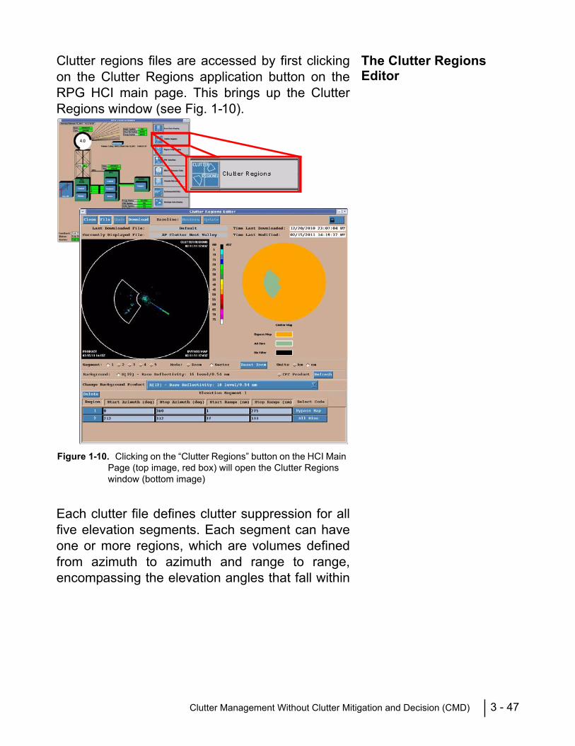
Clutter regions files are accessed by first clickingon the Clutter Regions application button on theRPG HCI main page. This brings up the ClutterRegions window (see Fig. 1-10).

Each clutter file defines clutter suppression for allfive elevation segments. Each segment can haveone or more regions, which are volumes definedfrom azimuth to azimuth and range to range,encompassing the elevation angles that fall within

Figure 1-10. Clicking on the “Clutter Regions” button on the HCI Main Page (top image, red box) will open the Clutter Regions window (bottom image)


that elevation segment (see Fig. 1-11). Eachclutter file can have up to 25 regions defined.

For the example Clutter Regions file in Figure1-12, assume that segment 1 has the Bypass Mapin control everywhere (Region 1), with one area ofAll Bins to the northeast (Region 2), and another tothe southeast (Region 3). The clutter file in Figure1-12 has 3 regions in segment 1, 2 regions insegment 2, and 1 region in segments 3 through 5.There are 8 regions total defined for this file.

The two lines of text at the top of the ClutterRegions Editor window, shown in Fig. 1-13 onpage 3-49, help you keep track of which file isdisplayed on the window, and which file was lastdownloaded to the RDA. The first line indicates thename of the clutter file that was last downloaded tothe RDA and at what time it was downloaded. The

Figure 1-11. Clutter regions are defined in the bottom section of the Clutter Regions file display.

Figure 1-12. Sample clutter regions file with eight total regions. A clutter regions file can have up to twenty-five regions.


next line tells you which clutter file is currentlydisplayed on the window.

Within each clutter file displayed, the configurationfor each of the five segments is available. Figure1-14 shows Segment 1, the lowest segment. Anyregion that is defined needs a Select Code, eitherBypass Map or All Bins.

In line 1, which should be the same for everyclutter file, there is a region from 0 to 360 degreesand from 1 to 275 nm, which is everywhere, withthe Bypass Map in control.

After line 1, which has the Bypass Map in controleverywhere, additional regions can be defined withAll Bins if needed. If there are areas with

Figure 1-13. The top of the display indicates which file is displayed and the last file downloaded to the RDA.

Figure 1-14. Each region needs a Select Code, either Bypass Map or All Bins (yellow box on right). A region is defined by start and stop azimuths and start and stop ranges.


predictable AP Clutter, files can be defined inadvance and downloaded as needed. Forexample, diurnal AP frequently occurs in valleysand over bodies of water, so the associated APclutter is in a predictable location. Otherwise,regions that apply All Bins must be defined asneeded before downloading to the RDA.

Bypass Maps are generated offline, stored, and donot update until new maps are generated. BypassMaps should be generated under propagationconditions that are “normal” for a given site. Thismeans no AP or precipitation going on. It isrecommended that Bypass Maps be checkedperiodically for relevance, and updated at leastseasonally.

The list of available clutter regions files isaccessed from the File button at the top of theClutter Regions window (see Fig. 1-15). Thestrategy for identifying clutter without CMDinvolves downloading existing files and creatingnew ones as needed. The Default file is a pre-defined file that cannot be deleted. It is part of thebaseline and designed to apply Bypass Mapfiltering for all azimuths and elevations. It isintended to be used for all non-AP situations.

Figure 1-15. Click the File button at the top of the Clutter Regions Editor window to access the list of available clutter regions files.


Pre-defined clutter regions files that addresspredictable locations for AP clutter, such as the“AP Clutter West Valley” file, are recommended.

To download a clutter file to the RDA, it must firstbe displayed at the Clutter Regions window. Clickon the name of the file, select Open, and the filewill be displayed. Once it is displayed on theClutter Regions Editor window, it can then bedownloaded to the RDA by clicking the downloadbutton at the top of the Clutter Regions Editorwindow (see Fig. 1-16).

In this example, the file “AP Clutter West Valley”has been displayed and is ready for download.

Clutter Management Conclusion

Bypass Maps will need to be generated oftenenough to keep them representative. Havingpredefined clutter files to address predictableareas of AP clutter is recommended. In general,clutter management without CMD requires pro-active downloading of clutter files. The Default fileis recommended when there is no AP present, andnew files can be created and downloaded asneeded to address AP clutter.

Figure 1-16. Once the correct Clutter Regions file has been selected, it can be downloaded to the RDA by clicking the Download button (yellow box).

3 - 52 Product Resolution

Product Resolution RPG Build 12.2 brings a change in the rangeresolution to some products. Super Resolutionmeans an azimuthal resolution of 0.5° and it is stilllimited to Z, V and SW on the Split Cut elevations.The display range for the Split Cut V and SWproducts is out to 300 km (162 nm) or 70 kft,whichever comes first. The remainder of the SplitCut products, including all the new dual-polproducts, have an azimuthal resolution of 1.0° anda range resolution of 0.25 km. Figure 1-17 showsthe difference in resolution between the Z, V andSW Split Cut elevations (top row) and differentialreflectivity and correlation coefficient (bottom row).

Z V SW

ZDR CC

Figure 1-17. For the Split Cut elevations, Z (upper left), V (middle), and SW (upper right) have 0.5 azimuthal resolution, while ZDR (lower left) and CC (lower right) have 1.0° azimuthal resolution.

Product Resolution 3 - 53

Split CutsThe Split Cut elevation dual-pol base data thatarrives from the RDA has an azimuthal resolutionof 0.5°. The left image in Figure 1-18 is the “raw”CC data from the RDA. It is too noisy for bothhuman interpretation and algorithm ingest. At theRPG, the dual-pol base data are first recombinedto 1° azimuth. The recombination is performed oneach channel separately: recombine H power,then recombine V power, then the crosscorrelation is recombined. The ZDR, CC, and ΦDPbase data are all recombined to 1° azimuth. Thesmoothing is done by the RPG Dual-PolPreprocessor.

Figure 1-18. Dual-pol base data arrives from the RDA with 0.5o azimuthal resolution (left) and is recombined to 1o azimuthal resolution (right).

CC CC

3 - 54 The RPG Dual-Pol Preprocessor

Batch Elevations andAbove

For the base and derived products of the Batchelevations and above, the azimuthal resolution is1.0° (see Fig. 1-19). The range resolution is 0.25km, which is an increase in resolution for manyproducts for these elevations. Also, the V and SWproducts have a display range out to 300 km (162nm) or 70 kft, whichever comes first.

The RPG Dual-PolPreprocessor

The RPG Dual-Pol Preprocessor prepares thedual-pol base data for base product generationand for input into the dual-pol algorithms: theHydrometeor Classification Algorithm (HCA), theMelting Layer Detection Algorithm (MLDA), andthe Quantitative Precipitation Estimation Algorithm(QPE).

The “raw” dual-pol base data are noisy inappearance. For any given range bin, the

Figure 1-19. Base and derived products of the Batch elevations and above have an azimuthal resolution of 1.0o and a range resolution of 0.25km.

Z V

ZDR CC

The RPG Dual-Pol Preprocessor 3 - 55

Preprocessor smoothing technique applies alinear average to a segment (of varying length) ofdata along the radial. This average value is thenassigned to the original range bin, which is at thecenter of the segment.

The remaining tasks for the Preprocessor arecomputing the Specific Differential Phase (KDP)values and Attenuation Correction.

Smoothing is also applied to the Z base data, butonly for input to the dual-pol RPG algorithms.There is no change to the Z values used togenerate all the base Z products.

Preprocessor and ZDR/CC

In Figure 1-20, the image on the left is raw ZDRfrom the RDA, which is not yet recombined orsmoothed. The image on the right is the samedata displayed in AWIPS after recombination andPreprocessor smoothing.

Figure 1-20. Raw ZDR (left) from the RDA is recombined and smoothed before it is displayed in AWIPS (right).


Figure 1-21 shows before and after preprocessingof correlation coefficient.

Preprocessor and ΦDP Since ΦDP is at the heart of dual-pol base data, itgets special treatment from the Preprocessor!

On the right in Figure 1-22 is an example of ΦDPvalues, which are not generated into a product atAWIPS. This image is from GR Analyst, showingthe raw Level II data. Once the ΦDP data havebeen smoothed, the Preprocessor calculates theKDP values. The KDP values are then availablefor generation of the KDP product (see Fig. 1-22,left) and for input to the dual-pol algorithms.

These two images are a good example of whyΦDP is not generated into a base product. It ismuch more difficult to interpret than KDP.

Figure 1-21. Raw CC (left) is recombined and smoothed (right) by the RPG Dual-Pol Preprocessor.

Figure 1-22. ΦDP values as seen in GR Analyst (right) and KDP values calculated by the Preprocessor (left).


As you may recall from the RDA training, ΦDP is aphase value which accumulates down radial (seeFig. 1-23). ΦDP has the greatest increase withrange where the beam encounters large amountsof liquid water.

You will likely see a data artifact that is related tohow ΦDP is processed along each radial,specifically in between segments of “weather.”

“Weather” is identified by CC>0.85. In the examplein Figure 1-23, there are two segments along theradial that are tagged as rain, because of theirassociated high CC values. Figure 1-23 showshow ΦDP typically behaves in “clear air”, but thereare exceptions.

Figure 1-23. This graphic shows how ΦDP values accumulate down radial.


Sometimes CC>0.85 is assigned to non-meteorological returns, such as residual clutternear the radar. This can then artificially increasethe ΦDP values down radial (see Fig. 1-24). Thereis an artifact that you will see on the ZDR and KDPproducts that is related to the behavior of ΦDPdown radial and another job of the Preprocessor:Attenuation Correction.

Attenuation Correction The final task of the Preprocessor is AttenuationCorrection for Z and ZDR. As before, the Z valuethat has this correction applied is only used for thedual-pol algorithms.

When the radar beam encounters high watercontent, the returned power can be attenuated,and ΦDP increases. The relationship between ΦDPand the amount of attenuation is strong enoughthat the increase in ΦDP can be used as anattenuation correction. Empirical relationshipshave been developed between ΦDP and the

Figure 1-24. Non-meteorological clutter can artificially increase ΦDP values down radial (red line).


attenuation of Z and between ΦDP and theattenuation of ZDR. These relationships arecurrently based on research in Oklahoma and willlikely be changed as knowledge from otherregions is gained.

ZDR and KDP SpikesIf you see spikes on ZDR and KDP, they areknown artifacts of the Preprocessor. There isresearch underway to adjust the Preprocessorparameters to minimize this artifact in the future.

The result is radially oriented spikes that aretransient in time and space as shown in Figure1-25. With ZDR, the spikes originate where thebeam encounters precipitation and persist withrange. This is due to ΦDP values that are too highwith respect to the ZDR values within theprecipitation. There is too much attenuationcorrection applied to ZDR, which then falselyincreases the ZDR values along these radials.

Figure 1-25. ZDR shows spikes where ΦDP values are too high with respect to ZDR values within precipitation.


With KDP, the spikes originate near the RDA,because of noisy ΦDP values (see Fig. 1-26). Thespikes in KDP usually smooth out if the beamintercepts precipitation. The best smoothingoccurs with rain only, since ΦDP behaves best inrain.

The ZDR and KDP spikes are more likely to occurwith residual clutter near the RDA. The need tomanage clutter manually (without CMD) will makethis more challenging in the short term. Thesespikes are most likely to occur on the lowerelevations. If there is rain at close range, spikesare rare, since ΦDP is well behaved in rain.

Figure 1-26. Spikes in KDP values can occur with noisy ΦDP values, but usually smooth out when the beam intercepts precipitation.

4 - 61

RPG Lesson 2: Hydrometeor Classification Algorithm (HCA) and Melting Layer Detection Algorithm (MLDA)

Until now, the only way to identify a melting layervia radar was to see a bright band in reflectivity,but it was never a guarantee that the bright bandwould be visible. With dual-pol radars, the meltinglayer stands out much more often in the productsof CC and ZDR because they have very uniquesignatures in the melting layer. The melting layermanifests itself as a ring (or partial ring) of lowerCC, typically around 0.9 to 0.95, and higher ZDR,somewhere between 0.5 and 2.5 dB. In thereflectivity image in Figure 2-1 there is not areadily visible bright band, but very prominentrings of lower CC and high ZDR.

Figure 2-1. An example of a bright bands that isn’t well-defined in Z (left), but is easily seen in CC (middle) and ZDR (right).

4 - 62

The Melting Layer Detection Algorithm (MLDA)uses these unique signatures of CC and ZDRwithin the melting layer to identify the heights ofthe top and bottom of the melting layer for eachradial. These heights are updated every volumescan and are used to produce a Melting Layer(ML) graphic product. The ML product is anoverlay and is available every volume scan forevery elevation angle (see Fig. 2-2).

Figure 2-3 shows the process of calculating theMLDA. The idea of the MLDA is to identify therings of CC and ZDR in an automated wayproviding the height of the top and bottom of themelting layer that is updated every volume scanand can be used by other algorithms such as theHydrometeor Classification Algorithm (HCA).

Figure 2-2. Image of the Melting Layer (ML) product.

Figure 2-3. Flow chart providing a high-level overview of how the MLDA works.

4 - 63

1. Inputs for the MLDATable 4-1 lists the inputs for the MLDA. Thealgorithm ingests radial-based data from theelevations of 4° through 10°. Below the 4°elevation angle, the signature of the melting layeris smeared due to beam broadening, thusaccurate detections are not possible. Above the10° elevation angle, there is little data. In additionto the radial-based data, the MLDA uses MLDAdata from previous volume scans. The number ofvolume scans used depends on the VCP mode(either precipitation or clear-air mode). Finally, adefault 0 Celsius height is ingested which eithercomes from a user-defined height set at the RPGor the height from the latest RUC model run.

2. Exclude Bins from Radial for Computation of Melting Layer Top/Bottom

The first step in the MLDA is to eliminate any binsin a radial that will not be used for identifying themelting layer top and bottom heights for that radial.Bins identified as ground clutter or biologicals bythe Hydrometeor Classification Algorithm (HCA)are excluded. Also, bins where the HCA isuncertain about a classification type, so eitheridentified as ND or UK, are excluded. Finally, binswhere the signal is too low (SNR < 5 dB) and anybins where the slant range height is above themaximum climatological height for a melting layer,which is set to 6 km (or 19 thousand feet), areexcluded.

Table 4-1: Inputs used to calculate the ML product.

4 - 64

The graphic in Figure 2-4 shows an example radialwhere bins meeting the exclusion criteria aremarked with a red X, and bins that will be used toidentify the melting layer top and bottom aremarked with a green check mark.

3. Compute WeightedValue for EachRemaining Bin

For each remaining bin from the previous step, theMLDA will compute a weighted value based on thelikeliness of that bin being within the melting layer.The MLDA uses Z, ZDR, CC and the elevationangle to compute this weighted value, and thehigher the weighted value, the more likely it is thatthe bin exhibits a melting layer signature.

As mentioned before, the motivation behind theMLDA is the observation that the ZDR increasesand CC decreases within the melting layerproducing rings of increased ZDR and decreasedCC coincident with the melting layer. The weightedvalue will be computed using this logic. Sincethese two rings are not always in the exact same

Figure 2-4. The algorithm filters bins according to their hydroclass, signal-to-noise ratio, and slant range height.

4 - 65

location, the algorithm will look at the given binand a few bins down radial from it and look for Zbetween 30 and 47 dBZ, ZDR between 0.8 and2.2 dB and CC between 0.9 and 0.97. If theseconditions pass, a non-zero value is assigned tothe given bin that is weighted according to itselevation angle. The higher the elevation angle,the higher the weight. This is because higherelevation data are less susceptible to beambroadening effects, giving a more accuratedepiction of where the melting layer is trulylocated.

4. Sort Weighted Values According to Their Height and Radial

Once all the valid bins have been assigned aweighted value, these values are sorted accordingto their height and radial into a height vs. radialarray with a vertical resolution of 0.1 km and radialresolution of 1 degree. A portion of an examplearray is shown in Figure 2-5.

The array is a combination of weighted valuesfrom the current volume scan and the previous 2volume scans for when the current volume scan isa precipitation VCP, and the previous 5 volumescans when the current volume scan is a clear-air

Figure 2-5. Portion of an example height vs. radial array

4 - 66

VCP. Keep in mind that the array is reset, or wipedclean, if the time between the current volume scanand the previous volume scan is greater than 30min.

5. Compute ML Top andBottom from Weighted

Values

Next, the MLDA computes the melting layer topand bottom heights for each radial from theweighted values if a threshold for the weightedvalues is met. As an example, for a given radial,the algorithm first sums all the weighted values ina window surrounding the given radial. Thiswindow includes the radials 10 degrees either sideof the given radial, and 1 km either side of theheight of the previous melting layer top. The sumis done from the bottom up. If this sum is above adefined threshold (i.e. 1500), which indicates thatthere are enough melting layer detections toconfidently identify a melting layer from the dual-pol data, the melting layer top and bottom arecomputed from the melting layer detections. Thebottom is defined as where the sum is 20% of thetotal sum, and the top is defined as where the sumis 80% of the total sum.

6. Fill in Missing Radials If the total sum from the previous step is below thedefined threshold (i.e. 1500), the melting layer topand bottom heights are not computed from themelting layer detections. The melting layer top andbottom will instead be generated by one of twoother methods. First, it will see if other radials inthe current scan had enough melting layerdetections to determine a melting layer top andbottom, and use the average top and bottomheights of those radials.

4 - 67

If no radials have a melting layer top and bottomheight determined from melting layer detections,then it will use the default 0 Celsius height definedeither in the Environmental Data Entry window, orby the latest RUC model. The top will be definedas the 0 Celsius height, and the bottom will be 500meters below that. It is recommended to have themodel update “On” as shown in Figure 2-6, as thiswill limit how often you will need to update theuser-defined 0 Celsius height seen in theEnvironmental Data Entry window (see Fig. 2-7).

Figure 2-6. The RUC Model is used if the MLDA cannot determine a melting layer from the available dual-pol data.

Figure 2-7. 0 Celsius height can be manually defined in the Environmental Data Entry window.

4 - 68 MLDA Adaptable Parameter

MLDA AdaptableParameter

There is one editable adaptable parameter withthe MLDA. Under the Algorithms window in theRPG, choose MLDA as the “Adaptation Item” (seeFig. 2-8).

This will display one URC parameter (seeFig. 2-9), which essentially allows the MLDA tocompute the heights from the dual-polarizationdata, which is what was just described, or to skipthat whole process and use only the input from theRPG Environmental Data instead. It is expectedthat the need to set this parameter to “No” willmost likely be seasonal.

The MLDA was developed primarily using warmseason events from central Oklahoma. However,some cool season events have been looked at and

Figure 2-8. The adaptable parameter associated with the MLDA can be found in the Algorithms window.

Figure 2-9. The adaptable parameter tells the MLDA whether or not to compute the heights from the dual-pol data.

Summary 4 - 69

it appears that when the melting level is near theground or there are two melting layers, thealgorithm has some issues and it is preferable tobypass the algorithm and use a uniform meltinglayer representative of the actual environment.

SummaryIn summary, we learned that the MLDA is basedon the unique signatures of CC and ZDR in themelting layer. It searches for bins exhibiting theseunique signatures from the elevations of 4°through 10°, and assigns a melting layer top andbottom height for each radial if there are enoughmelting layer detections. If there are not enoughmelting layer detections, it uses either the averagetop and bottom heights from the other radials inthe volume scan, or the default 0 Celsius heightdefined in the RPG. There is one editableadaptable parameter with this algorithm and it isused to determine whether the MLDA resultscome from the dual-pol data or from the RPGdefined 0 Celsius height.

Hydrometeor Classification Algorithm (HCA)

The dual-pol base products reveal additional, anduseful, information about the characteristics of thescatterers inside the radar resolution volumebeyond what the current legacy system alreadytells us. The Hydrometeor Classification Algorithm(HCA) works by using this additional information todetermine the dominant scatterer type within thatresolution volume. The product output by the HCAis called the hydrometeor classification (HC) and isproduced for every elevation angle.

4 - 70 Hydrometeor Classification Algorithm (HCA)

Before diving into the details of the HCA, here arethe 12 classes currently defined in the HCA (seeFig. 2-10): biological scatterers (BI), ground clutter/ anomalous propagation (GC), ice crystals (IC),dry snow (DS), wet snow (WS), light/moderate rain(RA), heavy rain (HR), big drops (BD), graupel(GR) and hail possibly mixed with rain (HA). Thelast two classifications are unknown (UK) and nodata (ND) and will be discussed later in thislesson. RF stands for range folding and is actuallynot part of the HC classification.

Figure 2-11 on page 4-71 shows a very high-leveloverview of how the HCA works. The HCA assignsa hydrometeor type for each radar bin based onthe dual-pol inputs. The dual-pol inputs arecombined to compute a likelihood value for eachhydrometeor type based on pre-defined thresholdsfor the various hydrometeor types, and thehydrometeor type with the highest likelihood valuewill be assigned to that bin.

Figure 2-10. HC product color legend from AWIPS display.

Hydrometeor Classification Algorithm (HCA) 4 - 71

1. Inputs for the HCAThe inputs for the HCA are listed in Table 4-2 onpage 4-71. For the base moments, reflectivity (Z)and velocity (V) are used. For the dual-polvariables, differential reflectivity (ZDR), correlationcoefficient (CC), differential phase (ΦDP), andspecific differential phase (KDP) are used. From Zand ΦDP, two texture parameters are computed:SD(Z) and SD(ΦDP). These variables have beenshown to be excellent discriminators between non-meteorological and meteorological echoes. Finally,two other inputs that are used are signal-to-noiseratio (SNR) in the horizontal channel, and themelting layer top and bottom heights asdetermined by the melting layer detectionalgorithm (MLDA).

Figure 2-11. High-level overview of how the Hydrometeor Classification Algorithm (HCA) works.

Table 4-2: Inputs used to calculate the HC product.


2. Determine AllowableClassifications

Hard Thresholds For any given range bin, the first step in thealgorithm is to determine which classifications areallowed based solely on the input data. There aretwo ways the algorithm does this. The first is byapplying hard thresholds. Table 4-3 lists thecurrent hard thresholds, and which classification isdeemed invalid based on the thresholds. Forexample, the classification for hail possibly mixedwith rain is invalid for a bin if the reflectivity isbelow 30 dBZ. There is a “special case” example,however, based on SNR. If SNR is below 5 dB fora bin, then all classifications are deemed invalid,and the bin is automatically set to ND and thealgorithm moves on to the next bin.

Table 4-3: Hard threshold for each hydrometeor classification.


Melting Layer LocationThe other method used to determine allowableclassifications is determining where the bin ofinterest is located relative to the melting layer.Figure 2-12 illustrates this method. First, the HCAdefines four heights based on the top and bottomof the melting layer which are labeled on the leftside of the graphic. They are the heights where:

• The top of the beam enters the bottom of themelting layer

• The center of the beam enters the bottom ofthe melting layer

• The center of the beam exits the top of themelting layer

• The bottom of the beam exits the top of themelting layer.

Where the radar bin falls relative to these heightsdetermines which classifications are allowed.

Figure 2-12. Graphic illustrating the method of using the melting layer to determine hydrometeor classification.


These regions are defined along with theallowable classifications in the graphic. Forexample, if a bin’s height falls in between theheight where the beam center has entered themelting layer bottom but has not crossed themelting layer top, this is defined as being “mostlywithin” the melting layer and the allowableclassifications are GC, BI, DS, WS, GR, BD, andHA.

3. Determine LikelihoodValues for the Allowable

Classifications

After the allowable classifications have beenidentified, the algorithm then iterates through eachallowable classification and calculates a likelihoodvalue for each of those classifications. Thatlikelihood value is a value ranging from 0 to 1 andis computed combining the following 3 factors:

• Membership functions

• Weighting factors

• Quality indices

Membership Functions Membership functions can be thought of as lookuptables. The purpose of these lookup tables is todetermine how likely a classification is based onan individual input. For example, hail typically haslow ZDR due to its tumbling nature, therefore, ifZDR is near zero for a bin, then the probability ofhail is high. Obviously, the other inputs need to belooked at in context, also. This will be done acouple steps later in the algorithm. At this point,the algorithm is just gathering information basedsolely on the individual inputs. NOTE: the lookuptables are based on research primarily conductedin central Oklahoma. Therefore, they may not beoptimal for all locations when the entire network isupgraded.


Weighting FactorsWeighting factors are used to determine whichinputs are best at discriminating the differenthydrometeor classifications. Table 4-4 lists theweighting factors used in the algorithm. Looking atground clutter (GC) and the input CC, theweighting factor is 1.0, but for Z, the weightingfactor is 0.2. This indicates that CC is much betterat discriminating GC than is Z. Again, like thelookup tables, the weighting factors have beenoptimized primarily using central Oklahoma cases.Therefore, these values may not be optimal for alllocations. These values, and the lookup tablevalues, are not yet editable adaptable parameters.It is not yet known which future RPG softwarebuild will provide these parameters in an editableformat.

Quality IndicesThrough extensive research it has been shownthat the accuracy of the dual-pol products must bequite good in order to reliably determine the mostlikely classification for a radar bin. Thus, thequality indices for Z, ZDR, CC, KDP and SD(Z)

Radar Variables

Hydro Class Type Z ZDR CC LKDP SD(Z) SD(ΦDP)

GC 0.2 0.4 1.0 0.0 0.6 0.8

BI 0.4 0.6 1.0 0.0 0.8 0.8

DS 1.0 0.8 0.6 0.0 0.2 0.2

WS 0.6 0.8 1.0 0.0 0.2 0.2

IC 1.0 0.6 0.4 0.5 0.2 0.2

GR 0.8 1.0 0.4 0.0 0.2 0.2

BD 0.8 1.0 0.6 0.0 0.2 0.2

RA 1.0 0.8 0.6 0.0 0.2 0.2

HR 1.0 0.8 0.6 1.0 0.2 0.2

HA 1.0 0.8 0.6 1.0 0.2 0.2

Table 4-4: Weighting factors used in the algorithm.


and SD(ΦDP) are used. These are values between0 and 1 that indicate the quality of each of thoseinputs with 0 meaning the quality is lacking to 1meaning the quality is excellent. The qualityindices for each of the above inputs are dependentupon some or all of the following characteristics:

• Attenuation

• Non-uniform beam filling

• Partial beam blockage

• Magnitude of the CC

• Receiver noise, or SNR

Compute OverallLikelihood Values

Next the algorithm puts the inputs in context withone another. It combines the lookup tableinformation with the weighting factors and qualityindices for all inputs and determines an overalllikelihood value for each allowable hydrometeortype. For example, suppose the allowableclassifications are ground clutter, biologicalscatterers, heavy rain, and hail possibly mixedwith rain. An overall likelihood for each of theseclassifications would be computed, and anexample is shown in Table 4-5.

4. Assigning aClassification

To determine which classification gets assigned bythe HCA, the algorithm iterates through eachclassification and finds the classification with themaximum likelihood value. For the exampleabove, iterating through these values, thealgorithm would determine that HA has the highestlikelihood value and would assign HA as theclassification for the HC product for that range bin.

GC BI HR HA

0.9861 0.7851 0.7761 0.9885

Table 4-5: Example of overall likelihood for ground clutter, biological scatterers, heavy rain, and hail.


5. Unknown Classification

There are two situations where the HCA willassign a classification of unknown, and this is thefinal step in the HCA. The first situation is in thecase of low data quality. If the maximum likelihoodvalue is below 0.4, this indicates that the dataused to compute the likelihood values wasprobably very poor, thus the classification will beset to unknown. Typical areas for this result arenear the radar in the absence of any real strongclutter or biological returns as seen in Figure 2-13(left) with all the pink bins in the HC product.

The other situation is in the case of overlappingcharacteristics. If the top two classifications havevery similar overall likelihood values and if thisdifference in likelihood values is less than 0.001,then the classification will be set to unknownbecause the algorithm cannot confidently decidewhich classification is dominant in that range bin.This will most likely be less common than the lowdata quality example, and is illustrated on the rightin Figure 2-13. Note the sparse bins of pink mixedin with the other bins identified as a dry snow, orgraupel, etc.

Max likelihood of < 0.4

Figure 2-13. Example of bin with a classification of “unknown” as a result of low data quality (left) and a bin with a classification of “unknown” as a result of an overlap in characteristics (right).

Difference between top two classifications is < 0.0001

4 - 78 Summary

Summary In summary, dual-polarization data revealadditional information about the characteristics ofprecipitation not previously shown by conventionalradar. The HCA works by using this additionalinformation provided by the base data todetermine a likelihood value for each pre-definedhydrometeor type. The hydrometeor type with thehighest likelihood value is tagged as thehydrometeor type for that range bin. If theconfidence in the decision is deemed too low, thenthe range bin gets tagged as unknown. To makesure some obvious misclassifications do not sneakthrough, some sanity checks are put in place. Forthe foreseeable future, there are no editableadaptable parameters associated with the HCA.

QPE and PPS in the RPG 5 - 79

RPG Lesson 3: Quantitative Precipitation Estimation (QPE) Algorithm

The Quantitative Precipitation Estimation (QPE)Algorithm applies the benefits of dual-pol to thevery complicated task of using a radar to estimaterainfall. For example, dual-pol can better identifyground clutter and biological targets which shouldnot be accumulated as rainfall. Range binsdominated by these non-precipitation returns areprevented from being converted to rainfall.

It will take time for QPE to reach it’s full potential.In the meantime, the legacy PrecipitationProcessing Subsystem (PPS) and all theassociated products will continue to be availablefor the foreseeable future.

QPE is run at the RPG, using both legacy anddual-pol base data. There are many similaritiesbetween the QPE and PPS, along with significantdifferences. QPE is also dependent on the resultsfrom the MLDA and the HCA, which werepresented in RPG Lesson 2.

QPE and PPS in the RPG

Figure 3-1 shows an overview of the data flow forboth the PPS and the QPE. The PPS is based onZ, V and SW base data, which are then processed

Figure 3-1. Overview of the data flow for both PPS and QPE.

5 - 80 QPE and PPS Product Data Levels

through a series of functions that result in the PPSsuite of rainfall products. PPS also includes a gagebias adjustment applied through the Adjustmentalgorithm.

All the base data (including the dual-pol variables)are available for MLDA, HCA and QPE, though theactual inputs vary. Specific inputs to QPE are: Z,ZDR, CC and KDP, as well as the results from theMLDA and the HCA. There is no gage biasadjustment yet implemented with QPE.

QPE and PPSProduct Data

Levels

Both the QPE and the PPS have one-hour rainfallproducts (see Fig. 3-2). One Hour Accumulation(OHA) is the dual-pol version of the legacy OneHour Precipitation (OHP) product. The data levelsfor the OHP have been editable at the RPG formany years. Now the data levels selected for theOHP also apply to the OHA product.

Similarly, both the QPE and the PPS have stormtotal rainfall products (see Figure 3-3 on page 5-81). Storm Total Accumulation (STA) is the dual-pol version of the legacy Storm Total Precipitation(STP) product. The data levels for the STP havebeen editable at the RPG for many years. Now thedata levels selected for the STP also apply to theSTA product.

Figure 3-2. Legacy and dual-pol One Hour rainfall product (yellow box) data levels are editable at the RPG.

Similar: Storm Total Accumulations 5 - 81

Similar: Storm Total Accumulations

The first similarity between the PPS and QPE ishow the storm total accumulations start and stop.For both algorithms, if the returns exceedthresholds of areal coverage and intensity,accumulations begin. Once the returns fall belowthe thresholds for one hour, accumulations stop.

PPS ParametersThe thresholds for the PPS shown in Figure 3-4should look familiar. RAINA is the areal coverage,while RAINZ is the intensity (in dBZ) threshold.RAINA and RAINZ are accessed from theAlgorithms window at the RPG under “HydrometPreprocessing”.

With the PPS, the total areal coverage of returnsthat exceed RAINZ are compared against RAINAevery volume scan. If RAINA is exceeded,

Figure 3-3. Legacy and dual-pol storm total rainfall product (yellow box) data levels are editable at the RPG.

Figure 3-4. RAINA and RAINZ (bottom yellow box) indicate the area coverage and intensity thresholds, which can be accessed from the Algorithms window under “Hydromet Preprocessing” (top yellow box).

5 - 82 Similar: Storm Total Accumulations

accumulations either begin or continue. Storm totalaccumulations reset to zero automatically whenreturns have been below RAINA and RAINZ forone hour.

QPE Parameters QPE uses the same concept for start and stop ofstorm total accumulations, but different thresholdnames. The QPE thresholds start with thePrecipitation Accumulation Initiation Function(PAIF). The PAIF Area Threshold is analogous toRAINA, while the PAIF Rate Threshold isanalogous to RAINZ. Though the units differ, thedefault values are the same as for the PPS. ThePAIF area threshold is 80 km2, while the PAIF ratethreshold is 0.5 mm/hr, which is equivalent to 20dBZ for Z = 300R1.4. The PAIF thresholds areaccessed from the Algorithms window at the RPGunder “Dual-Pol Precip” as shown in Figure 3-5.

PPS & QPE Storm TotalAccumulations

The initial recommendation is to set theparameters for both the PPS and the QPE to thesame values. RAINA is a threshold value thatvaries from site to site, and the PAIF AreaThreshold should be set to that same local value.Likewise, set the PAIF Rate Threshold to 0.5mm/hr, which matches the default RAINZ value of20 dBZ. When using a different RAINZ, dBZ willneed to be converted to mm/hr for the PAIF RateThreshold.

Figure 3-5. The PAIF Area and Rate Thresholds (lower yellow box) are analogous to RAINA and RAINZ, however rain rate values are expressed in mm/hr, not dBZ. These thresholds can be accessed through in the Algorithms window at the RPG under “Dual-Pol Precip.”

Similar: Storm Total Accumulations 5 - 83

With the thresholds set to the same values, theactual start and stop times of the PPS vs. the QPEare still expected to differ. This is because theQPE can better exclude clutter, biologicals, andhail from being converted to rainfall. However, theextent of any difference in start and stop times isnot yet known.

Both the QPE and the PPS have an automaticreset of the storm total accumulations after onehour of returns below their respective thresholds. Itis also possible to reset both the PPS and QPEaccumulations at the RPG.

From the RPG Control window, provide the URCpassword. This allows for a reset of the “LegacyPPS” and the “Dual-Pol QPE”. Either or both of theboxes can be selected, followed by clicking theActivate button just above as shown in Figure 3-6.

Figure 3-6. Storm total accumulations can be reset manually at the RPG for both PPS and QPE.

5 - 84 Similar: Exclusion Zones

Similar: ExclusionZones

Another similarity between the QPE and the PPSis the use of exclusion zones. There are movingground targets that are not filtered as clutter.Examples are rotating wind turbine blades andtraffic on roads. Returns from these targets usuallyexceed both the RAINZ and PAIF RateThresholds. Exclusion zones can be applied toboth the PPS and QPE, preventing this type ofradar return from being converted to rainfall.

Exclusion zones are set at the Algorithms windowfor Hydromet Preprocessing (PPS) and Dual-PolPrecip (QPE). Figure 3-7 on page 5-84 shows thelist for QPE, but the list of parameters for definingexclusion zones is the same for each algorithm.The recommendation for the initial use of both thePPS and the QPE is to set Exclusion Zoneparameters to the same values. It is expected thatQPE will better identify clutter, hail and biologicaltargets, but how that may translate to thesethreshold settings is not yet known.

Exclusion zones are an important tool, defining avolume from azimuth to azimuth, range to range,and up to a maximum elevation angle. The totalnumber of exclusion zones must also be defined.

Figure 3-7. Sample list of exclusion zones for QPE.

Different: One Hour Product 5 - 85

There is a misconception that exclusion zones“zero out” rainfall estimates within the zone. If arange bin falls within an exclusion zone, QPE andPPS just use the lowest elevation that is above theexclusion zone to estimate rainfall.

Figure 3-8 is an example of an event from theDodge City CWA. The reflectivity data (centerimage) are contaminated by a wind farm (circled)that is to the southwest of the radar. Level II datafrom the event has been processed by an RPGtwice. The STP product on the left was generatedwith an exclusion zone over the wind farm,eliminating false precipitation. The STP product onthe right was generated without the exclusionzone. Note the false precipitation that resultswithout the exclusion zone, especially the radiallyoriented structure.

Different: One Hour Product

There is a significant difference between the PPSand QPE on the generation of their respectiveone-hour products, the OHP and the OHA.

Figure 3-8. Example of reflectivity (center) contaminated by a wind farm (yellow circles). Images of STP with an exclusion zone (left) and without an exclusion zone (right) are also shown.

STP with exclusion zone STP without exclusion zone

5 - 86 Different: QPE Input

The behavior is the same for the beginning of anevent or the return of data to the RPG after anoutage. The beginning of an event means that thestorm total thresholds have been exceeded andaccumulations have begun. The return of data tothe RPG after an outage means that there hasbeen some kind of failure (wideband or RDA) thatprevents base data from getting to the RPG.

The difference, in either case, is that the PPS willnot generate an OHP for nearly one hour, whilethe OHA will be available beginning with thesecond full volume scan.

Different: QPEInput

In addition to the dual-pol base data, QPE usesthe output from the Hydrometeor ClassificationAlgorithm (HCA) and the Melting Layer DetectionAlgorithm (MLDA) to select rain rates for eachrange bin. HCA and MLDA help to prevent non-meteorological returns from being converted torain rate and to determine the best rain ratecomputation for the particular range bin.

Different: Pre-product Product

Both the PPS and QPE end up with rain ratesassigned to every range bin before the productsare built, but the respective methods are different.In terms of a “pre-product” product, the PPSproduces the Digital Hybrid Scan Reflectivity(DHR), which is the dBZ value for each range binbefore it is converted to rain rate. The QPEproduces the Digital Precipitation Rate (DPR),which is the rain rate for each range bin that isused for the product accumulations. Examples ofboth the DHR and the DPR are presented inFigure 3-9. The DPR product is also available forinput to FFMP.

Different: Pre-product Product 5 - 87

How QPE Builds DPREach WSR-88D has a local terrain file that is usedto determine the percentage of beam blockage.The PPS uses this file, and for any azimuth andrange that is determined to have >50% blockage,the next higher elevation angle is checked.

QPE has the benefit of Specific Differential Phase(KDP), which is immune to partial beam blockage.Thus QPE can use a lower elevation that hasgreater blockage. For any azimuth and range thatis determined to have >70% blockage, QPE thengoes to the next higher elevation angle.

Lesson 2 discussed how the HCA assigns aclassification to each range bin. If the bin isassigned biological, BI, the rain rate is set to 0.0and there is no additional search. It is assumedthat precipitation would not be present for anelevation above biological targets.

If the bin is assigned clutter (GC) or unknown(UK), QPE checks the same azimuth and rangeone elevation higher. The idea is to check forprecipitable echo above the clutter.

Figure 3-9. In terms of “pre-product” products, the PPS produces the Digital Hybrid Scan Reflectivity (DHR, left) and the QPE produces the Digital Precipitation Rate (DPR, right).

5 - 88 Different: Rain Rate Equations

QPE uses a higher elevation to compute a rainrate where:

• The HCA identifies clutter or unknown, or

• There is an exclusion zone in place, or

• The beam is > 70% blocked.

All of the remaining possible classification valuesare some type of precipitation. QPE uses theseclassification values and the height of the bin withrespect to the melting layer to determine a rainrate.

Different: Rain RateEquations

The three different QPE rain rate calculationmethods are each based on different inputs, andthe notation tells you the input. For example, R(Z)means the conversion is based on Z alone. Thefamiliar Z=300R1.4 can be represented asR(Z)=(0.017)Z0.714. For the QPE algorithm, thenotations R(Z), R(Z, ZDR) and R(KDP) are used tounderscore the input data for computing the rainrate. In some cases, R(Z) is used with a multiplier.

The objectives for this module do not involveremembering equations, but Figure 3-10 showsthe three equations for computing rain rate usedby QPE. The equations are included only to showa comparison of PPS vs. QPE approaches forconverting to rain rates.

Figure 3-10. Equations used to calculate rain rate used by QPE.

Different: Rain Rate Equations 5 - 89

The choice of equation is dependent on theclassification value and the height with respect tothe melting layer. For the R(Z,ZDR) equation, theZ and ZDR terms are in linear units (mm6/m3);they have not been converted to dB. The R(KDP)equation includes the possibility of a negative rainrate, however the QPE logic will reject R(KDP)when the rate is negative.

The coefficients and exponents for theseequations were developed based on researchconducted in Oklahoma. Additional research willbe needed to tune these equations for other areas.

The limitations of Z = 300R1.4, now presented in itsR(Z) format, are probably familiar. It oftenunderestimates rainfall in a warm rain dominantevent, while it overestimates the water at thesurface from mixed precipitation types, such aswet snow and hail.

R(Z,ZDR) is expected to perform better inconvection than stratiform rain. For a given Z, theassociated ZDR accounts for large drops (highZDR) in low concentration (low rain rate) vs. hailcontamination (high Z, but low ZDR).

R(KDP) has the advantage that KDP is mostlyimmune to partial beam blockage. In convectiveenvironments there is the risk of non-uniformbeam filling, which can result in lowered CC valuesdown radial from a storm core or a squall line.QPE does not use KDP values associated withCC<0.90, which can happen with non-uniformbeam filling.

There are a number of steps involved indetermining which rain rate is used, given the

5 - 90 QPE and Melting Layer

classification value and position of the range binwith respect to the melting layer.

QPE and MeltingLayer

Recall that the HCA uses the melting layer to helpdetermine what classifications are possible.Because the QPE uses HCA and applies amodified R(Z) relationship above the melting layer(2.8 * R(Z)) and just R(Z) below the melting layer,this causes a hard transition to appear near themelting layer in the QPE products. For example,Figure 3-11 shows the reflectivity and STA productfrom a rather long stratiform precipitation event.Notice the sharp transition in the STA productdepicted by the red arrow.

QPE & R(Z,ZDR) For Heavy Rain (HR) and light to moderate rain(RA), R(Z,ZDR) is used. Ideally, R(Z,ZDR) allowsZ and ZDR to balance one another. For example,an environment with large drops is oftenoverestimated by Z alone. The ZDR term would belarge because of the drop size, decreasing the rainrate.

The R(Z,ZDR) relation has thus far shown the bestperformance with continental rain events, with

Figure 3-11. The use of R(Z) below the melting layer and 2.8R(Z) above can cause a discontinuity in the QPE product (red arrow).

QPE and Bright Band Contamination 5 - 91

poorer performance for tropical events. In thetropical environment, a large number of smalldrops can make for very high efficiency rainfall,while the associated Z value is oftenunderestimated. Since the ZDR is going to be lowfor small drops, it is less likely to compensate byincreasing the rain rate.

QPE and Bright Band Contamination

Bright band contamination has long been achallenge for using a radar to estimate rainfall. TheQPE approach is to adjust the rain rate equationfor water coated frozen hydrometeors such as wetsnow that are typically located within a mesoscalemelting layer (stratiform rain event). A multiplier of0.6 is applied to the R(Z) relationship for the WSbins.

The bright band will still be apparent on Z or CC(see Fig. 3-12), but the overestimated Z will bemitigated before conversion to rain rate.

QPE and Hail Contamination

With the legacy PPS, hail contamination ismitigated by imposing a cap on the maximum rainrate used for accumulations. The limitation to thismethod is that there are many possiblecombinations of rain/hail mixtures, with manypossible associated Z values. With QPE, the first

Figure 3-12. Z, CC and ZDR images of a brightband which can contaminate rainfall estimates. The QPE aims to adjust for this.

5 - 92 QPE and Non-Uniform Beam Filling

step is that range bins that are likely to contain hailor graupel are first identified by the HCA. Theapproach is to use 0.8R(Z), which lowers the rainrate by the 0.8 multiplier, or to use R(KDP). KDP isthe dual-pol variable that indicates the magnitudeof liquid water content. The presence of hail or thesize of hail has little impact on the KDP value, so itis a good choice for conversion to rain rate.

QPE and Non-Uniform Beam

Filling

The artifact of a swath of low CC values due tonon-uniform beam filling can be either easy to spotor subtle. Comparing it to other radar data andunderstanding the environment may help evaluatewhether the CC values make sense.

It is important to be mindful of this artifact becauseCC affects the classification value that getsassigned, which then affects whether or nor rainfallis accumulated. In Figure 3-13, biological targetsare identified by the HCA, and QPE assigns norain rate to bins with the Biological classificationvalue.

Figure 3-13. Non-uniform beam filling effects can trickle down through other products, eventually affecting the QPE.

QPE and ZDR Calibration 5 - 93

There is no impact to the PPS that is as apparentas this swath of no rain. However, non-uniformbeam filling is often accompanied by beamattenuation, which can lower the PPS estimates.

QPE and ZDR Calibration

The QPE logic and parameter design was basedon an assumption of ZDR values that arecalibrated to within ±0.1 dB. At the time of thiswriting, it is not known if that level of accuracy hasbeen achieved. This will be an area of intenseinvestigation for the foreseeable future.

QPE StrengthsThe strengths of QPE listed below are mostlybased on using the benefits of dual-pol to mitigatelong-standing challenges with using any radar toestimate rainfall.

• Preventing returns from non-meteorologicaltargets from conversion to rainfall is well sup-ported by the dual-pol identification of groundclutter and biological returns

• Three different rain rate equations that areapplied bin-by-bin based on the classificationvalue

• Mitigation of bright band contamination

• Mitigation of hail contamination

• Rain rate product is generated every volumescan

QPE LimitationsAs with most new algorithms, there are a numberof limitations to QPE (listed below) that will likelyimprove over time.

• Many of the QPE parameters are based onresearch in Oklahoma, and regional “tuning” isexpected as dual-pol is fielded throughout theU.S.

5 - 94 Ongoing QPE Research

• Non-uniform beam filling has a unique impacton dual-pol base data, which translates to theQPE performance

• QPE performance is highly dependent on ZDRcalibration

• If an assigned classification value is invalid,that will increase the error of the rainfall esti-mate

• In long term stratiform events, the QPE prod-ucts are likely to show a discontinuity at the topof the melting layer

Ongoing QPEResearch

QPE is a very promising algorithm, thoughadditional research is needed to improveperformance. Though ZDR accuracy is sufficientfor human interpretation, improving ZDRcalibration is, and will continue to be, a highpriority for QPE.

QPE parameter adjustment is needed for threereasons.

1. Optimize performance for multiple regions out-side of Oklahoma

2. Identify and compensate for non-uniformbeam filling

3. Improve performance of the R(Z,ZDR) rela-tionship for tropical events

Research is likely to be needed to mitigate orsmooth the discontinuity on QPE products at thetop of the melting layer.

Date post:	27-Jan-2017
Category:	Documents
Upload:	vuduong
View:	247 times
Download:	5 times

Dual-Polarization Radar Principles and System Operations

Documents