THE EFFECT OF BAFFLES AND ENTRANCE PORTS ON THE MEASURED

REFLECTANCE OF DIFFUSE AND SPECULAR SAMPLES IN THE

INTEGRATING SPHERE

Thesis

Submitted to

The School of Engineering of the

UNIVERSITY OF DAYTON

In Partial Fulfillment of the Requirements for

The Degree of

Master of Science in Electro-Optics

By

K. V. Duncan-Chamberlin

UNIVERSITY OF DAYTON

Dayton, Ohio

May, 2015

ii

THE EFFECT OF BAFFLES AND ENTRANCE PORTS ON THE MEASURED

REFLECTANCE OF DIFFUSE AND SPECULAR SAMPLES IN THE

INTEGRATING SPHERE

Name: Duncan-Chamberlin, Katherine V.

APPROVED BY:

____________________ ____________________ Joseph W. Haus, Ph.D. William F. Lynn, M.S. Advisory Committee Chairman Innovative Scientific Solutions, Inc.

Technical Director, LOCI Principal Investigator, AFRL/RXAP Optical Measurements Electro-Optics Program Facility _____________________ Partha Banerjee, Ph.D. Committee Member Department Chair ____________________ ____________________ John G. Weber, Ph.D. Eddy M. Rojas, Ph.D., M.A., P.E., Associate Dean, School of Engineering Dean, School of Engineering

iii

ABSTRACT

THE EFFECT OF BAFFLES AND ENTRANCE PORTS ON THE MEASURED

REFLECTANCE OF DIFFUSE AND SPECULAR SAMPLES IN THE

INTEGRATING SPHERE

Name: Duncan-Chamberlin, Katherine V. University of Dayton Advisor: William Lynn, M.S.

Integrating spheres have many applications ranging from the measurement of

reflectance of materials to the calibration of imaging devices. While there have been

several works published that put forth integrating sphere theory and characterize

reflectance measurements within integrating spheres, very few have considered the

characterization of specular samples and or have incorporated a baffle.

In this work, a set of form factors are determined in order to create a model which

will allow us to predict the spectral behavior of samples within an integrating sphere

featuring a baffle mounted on the interior sphere wall. This model is evaluated using

samples of known reflectance values and shows good agreement with the known data.

However, error is present due to assumptions made in the calculation of two of the form

factors, the uncertainty in the reflectance of the sphere materials, as well as several

iv

simplifications made in modeling of the sphere geometry. Future work may improve the

model by identifying all sources of error and determining how to compensate for them.

v

ACKNOWLEDGMENTS

I would like to heartily thank my advisor, Bill Lynn, for his incredible patience

with me and for his guidance every step of the way during my research and penning of

my thesis. He also created the Visual Basic script used in calculating several of the form

factors reported herein, for which I am deeply grateful. Thanks also to Joseph Haus for

his support and for his willingness to serve as committee chairman upon short notice. I

also received direction and encouragement from department chair and committee member

Partha Banerjee, who kindly endured more than his fair share of worried and confused

emails. Recognition is also in order for my classmate Diane Beamer who weathered this

program with me and with whom I shared ideas.

Finally, I wish to thank the two individuals I share my home with: my treasured

cats Ebenezer and Kirk. Though having an attention-seeking animal land unexpectedly

in my lap while attempting to create this report frequently proved distracting, it is their

affection which has supported me throughout this endeavor and relieved the inherent

stresses.

vi

TABLE OF CONTENTS

ABSTRACT........................................................................................................................iii

ACKNOWLEDGEMENTS.................................................................................................v

LIST OF FIGURES............................................................................................................vii

LIST OF TABLES.……………………………………………………………………...viii

CHAPTER ONE: INTRODUCTION.................................................................................1

CHAPTER TWO: PRINCIPLES OF RADIOMETRY, FORM FACTORS,

AND INTEGRATING SPHERES.......................................................................................4

2.1 Form Factors in General.....................................................................................4

2.2 Integrating Spheres.............................................................................................8

2.3 Experimental.....................................................................................................12

2.4 Form Factor Calculations.................................................................................14

CHAPTER THREE: MODEL RESULTS........................................................................19

3.1 Results..............................................................................................................19

CHAPTER FOUR: CONCLUSIONS…….......................................................................24

REFERENCES...................................................................................................................26

APPENDIX ….................................................................................................................27

vii

LIST OF FIGURES

Figure 1. General form factor representation.......................................................................6

Figure 2. Original integrating sphere model........................................................................9

Figure 3. Revised integrating sphere model......................................................................10

Figure 4. Reflectance data for an Inconel mirror relative to a specular and diffuse

sample................................................................................................................................14

Figure 5. Form factor geometry for the elements partially blocked by the baffle............17

Figure 6. Input spectra for the model................................................................................21

Figure 7. Model output for a barium sulfate baffle...........................................................22

Figure 8. Model output for a Spectralon® baffle...............................................................23

viii

LIST OF TABLES

Table 1. Symbols, units, and definitions for radiometric terms…………………………..4

1

CHAPTER ONE

INTRODUCTION

Integrating spheres, sometimes referred to as Ulbricht spheres, are hollow spheres

with the notable feature that light is diffused uniformly inside. They are generally

constructed with a couple of ports allowing for incident light to be introduced and for

data to be collected using a detector. They have a range of applications, such as

measuring the reflectance of materials, providing a uniform light source, or aiding in

calibration of imaging devices [1].

Prior to the work of Jacquez and Kuppenheim [2], integrating spheres were

treated primarily by assuming that their aperture sizes were negligible and were thus

ignored. They presented theory in which the sphere was modeled with three ports and

determined irradiance values for a perfectly diffuse sample. In the following year,

Jacquez [3] found that by decreasing an integrating sphere's size, its efficiency would

increase, something which was further explored for a sphere with nonuniform coating [4].

They also recognized that most samples are not perfectly diffuse and that the sample

reflectance was dependent upon angle of incidence. The comparison and substitution

methods were compared by Jacquez and Kuppenhiem [5] with the comparison method

being demonstrated as clearly superior. They also discuss what effect the specular

component of light reflected off the sample has on producing error. Improvements to

2

their work are presented for flat, diffuse samples by Tardy who elaborated upon their

integration based methodology [6]. In 1965, Hisdal developed a new method of finding

reflection values for both perfectly diffuse and perfectly specular samples that greatly

simplified the mathematics involved without significantly impacting the accuracy of the

values derived [7]. The Hisdal matrix method is the foundation for this work because of

the simplicity it offers. It makes use of form factors to arrive at a value for reflectance.

Form factors (also known as view, configuration, shape, exchange, F, angle, or

geometry factors) represent the fraction of energy radiated by a surface and incident on a

second surface or itself. Form factors are used in gaining a better understanding of the

radiative properties of a material [8], and are also used in studying heat transfer. These

factors can therefore adequately describe the interaction between elements in an

integrating sphere.

While work has been performed on characterizing form factors which are

applicable to the measurement of reflectance of samples within integrating spheres, the

effect of a baffle inside an integrating sphere has been largely unexplored. A baffle is

used in order to block the first bounce of light from a diffuse sample from striking the

detector. Because measurements taken are relative values, the first reflection cannot be

allowed to reach the detector as this would be an absolute measurement. As data is

recorded relative to the sphere wall, light must first reflect off the sphere wall before the

detector sees it. The sphere used in this work is composed of Spectralon®, and the baffle

is coated in barium sulfate. Specular and diffuse samples, as well as samples featuring

both specular and diffuse properties, are commonly studied using an integrating sphere.

Lambertian samples are uniformly diffuse. Using the Hisdal matrix method [7], this

3

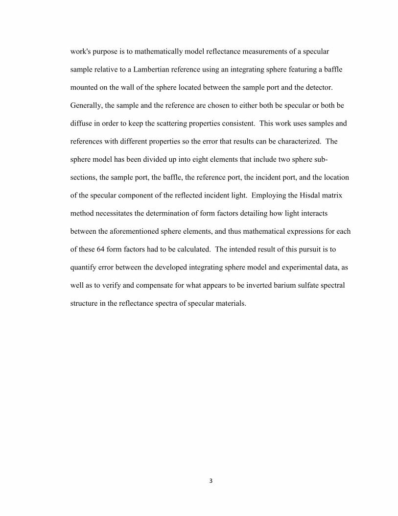
work's purpose is to mathematically model reflectance measurements of a specular

sample relative to a Lambertian reference using an integrating sphere featuring a baffle

mounted on the wall of the sphere located between the sample port and the detector.

Generally, the sample and the reference are chosen to either both be specular or both be

diffuse in order to keep the scattering properties consistent. This work uses samples and

references with different properties so the error that results can be characterized. The

sphere model has been divided up into eight elements that include two sphere sub-

sections, the sample port, the baffle, the reference port, the incident port, and the location

of the specular component of the reflected incident light. Employing the Hisdal matrix

method necessitates the determination of form factors detailing how light interacts

between the aforementioned sphere elements, and thus mathematical expressions for each

of these 64 form factors had to be calculated. The intended result of this pursuit is to

quantify error between the developed integrating sphere model and experimental data, as

well as to verify and compensate for what appears to be inverted barium sulfate spectral

structure in the reflectance spectra of specular materials.

4

CHAPTER TWO

PRINCIPLES OF RADIOMETRY, FORM FACTORS, AND INTEGRATING SPHERES

2.1 Form Factors in General

Before form factors are discussed, radiometric terms must first be introduced. A

summary of relevant terms is provided in Table 1. Flux, ϕ, represents the rate of change

of radiant energy, and the illuminance, E, is the flux per unit area. The luminous

emittance, L, is the total flux in all directions from a radiating differential area with

assumed uniform brightness.

Term Symbol Definition Radiometric

Energy U Joule (J)

Flux ϕ

t

U

Watt (W)

Luminous emittance* L

A

Wm-2

Illuminance E

A

Wm-2

*In some references, luminance emittance is symbolically represented by M. L is used to be consistent with Hisdal.

Table 1. Symbols, units, and definitions for radiometric terms.

A form factor represents the ratio between radiant flux leaving a specific surface

either by reflection or emission and striking another surface. Thus, it ranges between

5

zero and unity. It is a purely geometrical value and therefore has no dependence upon

temperature or surface properties, although incoming and outgoing energy must be

uniform across each surface and thus the surfaces have to be isothermal. The surfaces

considered are separated by air which is a nonparticipating medium and thus does not

interfere with the radiation as it passes through. The underlying assumption in form

factor theory is that the surfaces being studied are Lambertian. Generally, the form factor

from two differential areas dA1 and dA2 is given by

2221

2121

coscosdA

RdF dd

(2.1)

as illustrated in Figure 1 [9].

6

Figure 1. General form factor representation. Two differential areas separated by

distance R1-2 with angles θ1 and θ2 describing the angles between R1-2 and the surface

normals of the two surfaces respectively.

The reciprocity relation for form factors, which may be derived from Eq. 2.1, is

given by [9]

122211 FAFA (2.2)

where A1 and A2 are the areas of the two surfaces of interest, F1→2 is the form factor

describing energy transferred from A1 to A2 and, similarly, F2→1 is the form factor

describing energy transferred from A2 to A1. Because a set of form factors within an

enclosure is comprised of fractions of total energy and because the surfaces of the

7

enclosure have to collect all radiation going from one surface to all others, summing all

form factors in the set must result in unity as given by

N

jjiF

1

1 (2.3)

Further, any form factor describing radiation which leaves a surface and directly

strikes itself is zero in the case of a convex or planar surface as it is impossible in such

cases for the energy to return to itself due to form factors requiring a straight line path.

Each area has a luminous emittance, L, which is the total light power emitted per

unit area of the surface of a source of light. For a model with two surfaces, the luminous

emittance of the surface A1 may be defined as [7]

11212111111 ErFLrFLrL (2.4)

where

r1 - the reflectance associated with A1.

F11 and F21 - the form factors from A1 to itself, and A2 to A1 respectively.

8

E1 - the illuminance, which is the amount of light energy per unit area reaching A1

from an external source.

This equation is an accounting for each contributing factor to a curved surface

emitting light. The first term describes how the surface illuminates itself, the second term

accounts for how a second surface (A2) is illuminating it, and the third term is the source

which is illuminating it (incident beam) and thus reflecting off of it. This equation can be

expanded to describe any number of contributing areas in the same way up through

r1LnF1n, and likewise may be written as a system of equations for the n areas. This may

be represented as a matrix [7]

nnnnnnnnnnnn

n

n

n

Er

Er

Er

Er

L

L

L

L

FrFrFrFr

FrFrFrFr

FrFrFrFr

FrFrFrFr

33

22

11

3

2

1

321

33333323313

22232222212

11131121111

1

1

1

1

(2.5)

2.2 Integrating Spheres

Integrating sphere theory can be considered as a way to study the uniform

collection of all scattered light and measurement of the total hemispherical reflectance of

the sample rather than just the reflectance factor in one particular direction. It is of use to

model an integrating sphere by dividing it into several portions of interest and

considering how each of them reflect light (Figure 2).

9

Figure 2. Original integrating sphere model. The integrating sphere to be modeled

consists of eight different areas of interest. Areas 1 and 4 are hemispheres defined by the

baffle bisecting the sphere minus any other labeled areas. Area 2 is the sample port, 3 is

the photosensor, 5 is the incident port, 6 is the location of the first bounce of the specular

component of the incident last beam, and 7 and 8 are the baffle.

The matrix may be simplified by ignoring areas 3 and 6 as Hisdal does as their

areas are small compared to the others, instead treating light striking those areas as if it is

hitting the sphere wall (Figure 3). For the purposes of consistency, enumeration of form

factors is treated as if the two areas remain.

10

Figure 3. Revised integrating sphere model. The sphere diagram revised to neglect the

detector and the location of the first bounce of the specular component.

An integrating sphere was used in this work to perform reflectance measurements,

and there are two primary methods of measuring reflectances. These are known as the

substitution and comparison methods [2]. Substitution involves a sphere with just one

port that is used for measuring reflection. A measurement is taken relative to a standard,

and then the standard is removed and a sample is put in its place. However, in doing this,

the sphere has changed. With the sphere walls having unequal reflectances between the

two states (having the reference inserted and having the sample inserted), error in this

method is significant to the extent that the comparison method is accepted to be

11

altogether superior [5]. In the comparison method, both the reference and the sample are

present in the sphere at the same time, each with their own port. Thus, the relationships

between the inserted objects and the sphere walls are unchanged during measurement.

Instead, where the beam strikes is moved depending on whether the standard or the

sample is being measured. This is a much more accurate method than the substitution

method. However, this work employs a somewhat different method known as the Taylor

method which is an amalgamation of the substitution and comparison methods. This

employs two beams, one for the reference and one for the sample. One of these beams

comes through the reference port and strikes the sphere wall which is an intermediate

reference. The reference material is compared relative to the wall and then the sample is

compared relative to the wall, and then a ratio is taken of the results. Both measurements

taken are comparison measurements although it is like the substitution method in that the

standard is put into the sphere and then removed and replaced with the sample, and some

error may be introduced from making the second measurement, but it is not equivalent to

the substitution type error.

Hisdal develops a treatment for specular and diffuse samples [7]. Of interest is

his work on finite, flat, perfect specular samples, although he does not consider the effect

of a baffle. Incident light is completely reflected to another area within the sphere, and

this new area is treated as the sample area. This sample area will emit an excitation flux

as well as reflect excitation flux from the sample itself. Part of this is lost through the

entrance port which, like the photocell, is assumed to be perfectly absorbing as its

reflectance is zero. Although none of the materials used in our measurements have

constant brightness as a function of angle of incidence (Lambertian), they are treated as

12

such in order to simplify calculations. Because integrating sphere theory is largely

applicable only to diffuse materials, the assumption is made that when studying a

specular material, the specular component of reflected light bounces from the sample to

the area marked as 6 in Figure 2. After the light strikes area 6, it is then assumed that the

light is now diffuse. This may be done because more error is introduced during the first

reflection of light than ensuing reflections, because following the first reflection the light

undergoes scattering and this has an averaging effect. The first bounce results in scatter

off the sample, whereas the majority of ensuing reflections scatter off the sphere wall,

which produces more uniform data as the scatter off the sphere wall is different from the

scatter off the sample. Thus, after the first bounce, the sample is modeled as Lambertian.

Part of this work is evaluating whether or not this simplifying assumption is a valid one.

2.3 Experimental

Directional hemispherical reflectance was measured using a Perkin-Elmer

Lambda 9 UV/Vis/IR spectrophotometer with a custom integrating sphere. The Perkin-

Elmer is a double beam instrument. Using a double beam instrument permits the

measurement of data relative to a reference such that, in this case, the reference beam

strikes the sphere wall (which is an intermediate reference) and the sample beam

illuminates the sample. The reference material's reflectance is measured relative to the

sphere wall, and the sample's reflectance is also measured relative to the sphere wall.

The Perkin-Elmer was used to collect reflectance data from samples of Spectralon®,

barium sulfate, an Inconel mirror, and a National Research Council of Canada (NRC)

stainless steel mirror. The Inconel mirror's reflectance was measured relative to an NRC

standard and compared against reflectance data taken relative to SRS99, which is a

13

Spectralon® reference standardized using National Institute of Standards and Technology

(NIST) traceable procedures. The Inconel mirror and the NRC stainless steel mirror are

both specular materials, and thus the data taken when the Inconel mirror's reflectance was

measured relative to the stainless steel mirror has the higher accuracy. In contrast,

SRS99 is a diffuse material, and error is much higher when a specular sample is

measured relative to a diffuse reference due to their different scattering properties. As

illustrated in Figure 4, there are clear differences between the spectra.

The integrating sphere within the Perkin-Elmer is a floor-mount sphere made of

Spectralon® with a wavelength range of 250-2500 nm. Directional hemispherical

reflectance is subject to some errors such as using an improper reference. Using a NIST

standard will correct that, with the error then being related to the machine's precision.

Error can also come from noise, but can be lessened by decreasing spectral resolution.

There is also the possibility of port error when first bounce light does not exit the incident

port. There is a need for further study to more accurately characterize this error.

Data collection was performed using custom Perkin-Elmer software. A

background scan was run first to normalize the output to the reference spectrum. With

this stored in memory, the Perkin-Elmer is then ready to take reflectance data on a

sample. Each sample was prepared and then mounted in the center of the sample holder

after removing the SRS99 reference. Measurements can then be performed on the sample

and a correction factor can be applied via the software. This ratios the sample data and

the reference data in order to remove the reflectance of the sphere wall.

14

0.50

0.55

0.60

0.65

0.70

0.75

0.80

0.85

0.90

0.95

1.00

1000 1100 1200 1300 1400 1500 1600 1700 1800 1900 2000 2100 2200 2300 2400 2500

Wavelength (nm)

Ref

lect

ance

Inconel

Inconel vs SRS99

Figure 4. Reflectance data for an Inconel mirror relative to a specular and diffuse

sample. Reflectance data for an Inconel mirror taken relative to an NRC standard plotted

alongside data taken relative to a NIST standard.

2.4 Form Factor Calculations

36 form factors were determined to describe the six relevant sections of the

integrating sphere. They are described in Eq. 2.6.

In the case of F11, F22, F44, and F55 the derivation may be understood as the curved

surface acting on itself: thus, we consider the energy received in the area of interest

divided by the energy transmitted in area. Therefore, the numerator is proportional to its

own area, and because the sphere is Lambertian, the denominator is proportional to the

15

area of the entire sphere. The majority of the form factors, F12, F15, F21, F25, F51, and F52

may be thought of similarly, with the numerator being proportional to the receiving area

and the denominator again being proportional to the total area. For F14, F24, F54, F71, F72,

and F84 the factors were found by recognizing the sum of all the factors in the row must

be one using Eq. 2.3 and then subtracting all of the other (known) factors from one. F17,

F41, F42, F45, F72, F75, and F48 come from manipulating Eq 2.2, with the corresponding

form factor known. F18, F28, F47, F58, F74, F78, F81, F82, F85, and F87 are derived by

recognizing that the baffle blocks the line of sight between the two areas, and are thus

zero. F77 and F88 describe flat surfaces and are therefore zero. Factors F27, F38, F57, and

F68 are complicated by the presence of the baffle and must be solved using Eq 2.7 [10].

16

000100

0001

0171

0

0171

01

888785848281

787757

7

5757427

7

272887775747271

58575

5557555251542

521

51

84

4

8484754

4

545

44424

4

24214

4

141

28275

2527252221242

221

21

1871

1

717

5151715121114

212

111

FFFFFF

FFFA

AFFF

A

AFFFFFFF

FCFA

AFFFFFF

A

AF

A

AF

FA

AFFF

A

AF

A

AFF

A

AFF

A

AF

FCFA

AFFFFFF

A

AF

A

AF

FFA

AF

A

AFFFFFF

A

AF

A

AF

sss

s

sss

sss

(2.6)

where C17 denotes

(2.7)

2 2 2 2

1 21 1 1 1 1

2 21

1/2 1/22 2 2 2 2

1 222 2 12

2 2

11 , , ,

where

sin cos cos sintan

2 2 cos sin 2 cos

cos cossin tan

sin sin

i j k l

i j k li j k l

F G x yA

y x yG

x x x x

xy

y

11 22

22 2

2 2

cossin tan

sin

2 cosln

2 2 cos

x

y

x x yd

y x x

17

To use this equation, the sample port and incident port were approximated as

squares with areas matching their original values. The two surfaces of interest are treated

as two rectangles at an angle to each other (Figure 5). This equation was chosen because

it most closely matched the geometry of the two surfaces, but it is an approximation in

that it treats the port surfaces as rectangular rather than circular and also in that the baffle

is modeled as being perpendicular to the sphere wall rather than being mounted at an

angle.

Figure 5. Form factor geometry for the elements partially blocked by the baffle. One

surface is on the x axis and the other is along the ξ axis, sharing the vertical axis y. The

angle between them is α. x1 and x2 denote the starting and ending points of A1 along the

x axis, and y1 and y2 describe its starting and ending points along the y axis. Similarly,

for A2, ξ1 and ξ2 represent the width of the area and η1 and η2 give its height along the y

axis.

18

The visual basic script used to calculate F27 and F75 may be found in Appendix A.

This script was tested against values found in work by Krishnaprakis [10] and produced

identical results when α was 90 degrees and very close results at other angles. The form

factors are illustrated in Eq. 2.8.

000100

0000188.0009972.08984.0

000271.001456.048273.001196.048804.0

04322.0001447.048544.000765.044921.0

0175.001456.031044.001196.048804.0

003862.001456.044682.001196.048804.0

888785848281

787775747271

585755545251

484745444241

282725242221

181715141211

FFFFFF

FFFFFF

FFFFFF

FFFFFF

FFFFFF

FFFFFF

(2.8)

19

CHAPTER THREE

MODEL RESULTS

3.1 Results

To develop the model, Eq. 2.4 was rearranged to solve for the L matrix by

multiplying both sides by the inverse of the first matrix (Eq. 3.1).

nnnnnnnnnnn

n

n

n

n Er

Er

Er

Er

FrFrFrFr

FrFrFrFr

FrFrFrFr

FrFrFrFr

L

L

L

L

33

22

11

1

321

33333323313

22232222212

11131121111

3

2

1

1

1

1

1

(3.1)

The model was applied twice: once for the reference, and again for the sample.

For each case, r1 and r4 were the reflectance of optical grade Spectralon® as a function of

wavelength, r5 was the reflectance of the entrance port and thus zero, and r7 and r8 were

the reflectance of barium sulfate as a function of wavelength. r2 represents SRS99 in the

case of the reference and designates Inconel in the sample case. In the reference case,

only the second element of the illuminance matrix is of importance, and in the sample

case, only the third element (which corresponds to the fourth area) is needed. The

20

excitation flux is arbitrary and is set to zero for elements that are not of interest, and

determined via Eq. 3.2 for those which are [7].

5'66221

2

021 1 FFrrA

AErrE

fl

(3.2)

A2fl is the area of the sample, and A represents the area illuminated, which in this

case is the area of the hemisphere defined by the baffle bisecting the sphere (A4). When

Hisdal created his model, he simplified in part by ignoring the entrance port. The

bracketed term represents the loss due to this port. This port error is already accounted

for in the matrix presented in this work. If this term is included, the port error is

overcompensated for and model error is significantly increased as a result. The luminous

emittance of the sphere wall when the sample was illuminated (L'4) was then divided by

the luminous emittance of the sphere wall when the reference was illuminated (L4). This

ratio was then multiplied by the reference reflectance (r2) to get the reflectance (Eq 3.3).

2

4

'4 r

L

Lr (3.3)

The model resulted in absolute reflectance values diverging from known standard

values, although the spectral features generated were consistent. To compensate for this

21

error, a correction factor was introduced based upon known data at 1000 nm. This

correction factor, when multiplied by the value of the data point given by the model,

returns the known value. This makes it easier to evaluate how well the model predicts

the behavior of the spectra.

The input spectra are shown in Figure 6. The model was applied to the cases of a

baffle treated as if made of barium sulfate (Figure 7) and of Spectralon® (Figure 8).

0.750

0.775

0.800

0.825

0.850

0.875

0.900

0.925

0.950

0.975

1.000

1000 1100 1200 1300 1400 1500 1600 1700 1800 1900 2000 2100 2200 2300 2400 2500

Wavelength (nm)

Ref

lect

ance

Spectralon (Bulk Optical Grade)

SRS99

BaSO4 (Sample #3 High three)

Figure 6. Input spectra for the model. The reference reflectance data (bulk optical grade

Spectralon®), SRS99, and the average value of three experimentally obtained data sets for

barium sulfate.

22

0.50

0.55

0.60

0.65

0.70

0.75

0.80

0.85

0.90

0.95

1.00

1000 1100 1200 1300 1400 1500 1600 1700 1800 1900 2000 2100 2200 2300 2400 2500

Wavelength (nm)

Ref

lect

ance

Model Results

Inconel vs SRS99

Figure 7. Model output for a barium sulfate baffle. Model output for Inconel with a

barium sulfate baffle compared against known values.

23

0.50

0.55

0.60

0.65

0.70

0.75

0.80

0.85

0.90

0.95

1.00

1000 1100 1200 1300 1400 1500 1600 1700 1800 1900 2000 2100 2200 2300 2400 2500

Wavelength (nm)

Ref

lect

ance

Model Results

Inconel vs SRS99

Figure 8. Model output for a Spectralon® baffle. Model output for Inconel with a

Spectralon® baffle compared against known values.

The model is successful in reproducing inverted spectra. It was hypothesized that

this inverted spectra was due to either the baffle or the entrance port which change the

overall level of light inside the sphere. The model shows that the inverted spectra likely

results from the baffle since the spectral features more closely match barium sulfate than

Spectralon®. It's possible that the baffle is a combination of barium sulfate and

Spectralon® since the baffle should be opaque, and for Spectralon® to be opaque it must

be significantly thicker than the baffle is, and thus the baffle might be lightly coated in

barium sulfate.

24

CHAPTER FOUR

CONCLUSIONS

In order to model the effect on spectral behavior of measuring reflectance data of

a specular sample relative to a diffuse reference, a set of form factors was determined in

accordance with the Hisdal matrix method. This model also accounts for the presence of

a baffle inside the integrating sphere. Experimental data was input into the model and the

output was compared against known data, showing good agreement.

Several simplifying assumptions were made in developing the model. While

reflectance data was taken using the Taylor method, the model treated it as if it had been

collected using the substitution method. In addition, although none of the sphere

components produce Lambertian scattering, all materials are treated as if they are

Lambertian. Also, the model does not mimic the sphere's geometry, and the factors F27,

F72, F57, and F75 treat the ports as rectangles rather than circles, as well as treating the

baffle as bisecting the sphere when in reality it does not. Further, the reflectance values

of the sphere materials are not known exactly. Ideally, the sphere could be disassembled

and reflectance data could be taken for each component. Future work could ascertain

what model improvements are needed to lessen the error present in the model. More

accurate values of F27, F72, F57, and F75 should be determined, and the model should

reflect the true sphere geometry. Further, knowing the reflectance of the actual materials

is necessary, and may necessitate constructing a test sphere of known materials.

25

Additionally, the area corresponding to the location of the first bounce of specular light

(A6) was removed from consideration and treated as part of the hemisphere defined by

the baffle bisecting the sphere (A4). Accounting for A6 would improve the accuracy of

the model. Revision of the model to account for the usage of the Taylor method is also

recommended.

26

REFERENCES

[1] Labsphere, 'TECHNICAL GUIDE Integrating Sphere Radiometry and Photometry',

2015. [Online]. Available: http://www.labsphere.com/uploads/technical-guides/a-guide-

to-integrating-sphere-radiometry-and-photometry.pdf. [Accessed: 06- Nov- 2014].

[2] J. Jacquez and H. Kuppenheim, 'Theory of the Integrating Sphere', J. Opt. Soc. Am.,

vol. 45, no. 6, p. 460, 1955.

[3] J. Jacquez, W. McKeehan, J. Huss, J. Dimitroff and H. Kuppenheim, 'An Integrating

Sphere for Measuring Diffuse Reflectance in the Near Infrared', J. Opt. Soc. Am., vol. 45,

no. 10, p. 781, 1955.

[4] D. Goebel, 'Generalized Integrating-Sphere Theory', Applied Optics, vol. 6, no. 1, p.

125, 1967.

[5] J. Jacquez and H. Kuppenheim, 'Effect of Elimination of the Specular Component on

Efficiency and Error of the Integrating Sphere', J. Opt. Soc. Am., vol. 46, no. 6, p. 428,

1956.

[6] H. Tardy, 'Flat-sample and limited-field effects in integrating sphere measurements',

J. Opt. Soc. Am. A, vol. 5, no. 2, p. 241, 1988.

[7] B. Hisdal, 'Reflectance of Perfect Diffuse and Specular Samples in the Integrating

Sphere', J. Opt. Soc. Am., vol. 55, no. 9, p. 1122, 1965.

[8] J. Cabeza-Lainez, J. Pulido-Arcas and M. Castilla, 'New configuration factor between

a circle, a sphere and a differential area at random positions', Journal of Quantitative

Spectroscopy and Radiative Transfer, vol. 129, pp. 272-276, 2013.

[9] J. Howell, 'A Catalog of Radiation Heat Transfer Configuration Factors --

Introduction', Thermalradiation.net, 2015. [Online]. Available:

http://www.thermalradiation.net/intro.html. [Accessed: 18- Jan- 2015].

[10] C. Krishnaprakas, 'View Factor Between Inclined Rectangles', Journal of

Thermophysics and Heat Transfer, vol. 11, no. 3, pp. 480-481, 1997.

27

APPENDIX

Sub C_17_Calc() Dim alpha, pi As Double alpha = Range("C1").Value2 pi = 4 * Atn(1) alpha = alpha * pi / 180 Dim xx, yy, eeta As Double Dim x(2) As Double x(1) = Range("C2").Value2 x(2) = Range("C3").Value2 Dim y(2) As Double y(1) = Range("C4").Value2 y(2) = Range("C5").Value2 Dim eta(2) As Double eta(1) = Range("C11").Value2 eta(2) = Range("C12").Value2 Dim xi(2) As Double xi(1) = Range("C8").Value2 xi(2) = Range("C9").Value2 Dim Area1 As Double Area1 = (x(2) - x(1)) * (y(2) - y(1)) Dim Area2 As Double Area2 = (xi(2) - xi(1)) * (eta(2) - eta(1)) Dim Sum, F, G, delta, aa, aa1, aa2, bb, cc, dd, ee, ff, gg, hh, ii As Double G = 0 F = 0 Dim m, p As Long p = Range("C14").Value2 For i = 1 To 2 xx = x(i)

28

'MsgBox "xx equals " & xx & "" For j = 1 To 2 yy = y(j) 'MsgBox "yy equals " & yy & "" For k = 1 To 2 eeta = eta(k) 'MsgBox "eeta equals " & eeta & "" Sum = 0 delta = (xi(2) - xi(1)) / p xxi = xi(1) For l = 1 To p aa1 = (xx - xxi * Cos(alpha)) * Cos(alpha) - xxi * Sin(alpha) ^ 2 aa2 = (xx ^ 2 - 2 * xx * xxi * Cos(alpha) + xxi ^ 2) ^ (0.5) * Sin(alpha) ^ 2 aa = aa1 / aa2 bb = (eeta - yy) / aa2 cc = Cos(alpha) / ((eeta - yy) * (Sin(alpha)) ^ 2) dd = (xxi ^ 2 * (Sin(alpha)) ^ 2 + (eeta - yy) ^ 2) ^ (0.5) ee = (xx - xxi * Cos(alpha)) / dd ff = xxi * Sin(alpha) * Atn((xx - xxi * Cos(alpha)) / Sin(alpha)) gg = xxi / (2 * (eeta - yy)) hh = (xx ^ 2 - 2 * xx * xxi * Cos(alpha) + xxi ^ 2 + (eeta - yy) ^ 2) / (xx ^ 2 - 2 * xx * xxi *

Cos(alpha) + xxi ^ 2) ii = ((eeta - yy) * (Sin(alpha)) ^ 2) / (2 * pi) Sum = Sum + (aa * Atn(bb) + cc * (dd * Atn(ee) - ff) + gg * Log(hh) / Log(2.718282)) * delta / 6 xxi = xxi + delta / 2 aa1 = (xx - xxi * Cos(alpha)) * Cos(alpha) - xxi * Sin(alpha) ^ 2 aa2 = (xx ^ 2 - 2 * xx * xxi * Cos(alpha) + xxi ^ 2) ^ (0.5) * Sin(alpha) ^ 2 aa = aa1 / aa2 bb = (eeta - yy) / aa2 cc = Cos(alpha) / ((eeta - yy) * (Sin(alpha)) ^ 2) dd = (xxi ^ 2 * (Sin(alpha)) ^ 2 + (eeta - yy) ^ 2) ^ (0.5) ee = (xx - xxi * Cos(alpha)) / dd ff = xxi * Sin(alpha) * Atn((xx - xxi * Cos(alpha)) / Sin(alpha)) gg = xxi / (2 * (eeta - yy)) hh = (xx ^ 2 - 2 * xx * xxi * Cos(alpha) + xxi ^ 2 + (eeta - yy) ^ 2) / (xx ^ 2 - 2 * xx * xxi *

Cos(alpha) + xxi ^ 2) ii = ((eeta - yy) * (Sin(alpha)) ^ 2) / (2 * pi) Sum = Sum + 4 * (aa * Atn(bb) + cc * (dd * Atn(ee) - ff) + gg * Log(hh) /

Log(2.718282)) * delta / 6

29

xxi = xxi + delta / 2 aa1 = (xx - xxi * Cos(alpha)) * Cos(alpha) - xxi * Sin(alpha) ^ 2 aa2 = (xx ^ 2 - 2 * xx * xxi * Cos(alpha) + xxi ^ 2) ^ (0.5) * Sin(alpha) ^ 2 aa = aa1 / aa2 bb = (eeta - yy) / aa2 cc = Cos(alpha) / ((eeta - yy) * (Sin(alpha)) ^ 2) dd = (xxi ^ 2 * (Sin(alpha)) ^ 2 + (eeta - yy) ^ 2) ^ (0.5) ee = (xx - xxi * Cos(alpha)) / dd ff = xxi * Sin(alpha) * Atn((xx - xxi * Cos(alpha)) / Sin(alpha)) gg = xxi / (2 * (eeta - yy)) hh = (xx ^ 2 - 2 * xx * xxi * Cos(alpha) + xxi ^ 2 + (eeta - yy) ^ 2) / (xx ^ 2 - 2 * xx * xxi *

Cos(alpha) + xxi ^ 2) ii = ((eeta - yy) * (Sin(alpha)) ^ 2) / (2 * pi) Sum = Sum + (aa * Atn(bb) + cc * (dd * Atn(ee) - ff) + gg * Log(hh) / Log(2.718282)) * delta / 6 Next m = i + j + k G = -ii * Sum 'MsgBox "G equals " & G & "" F = F + ((-1) ^ m) * G 'MsgBox "F equals " & F & "" Next Next Next F = F / Area1 MsgBox "Form Factor C-17 equals " & F & "" End Sub