Durable Dominance: Dominant Entrenchment through...

October 10, 2013

Durable Dominance:

Dominant Entrenchment through Open Competition

Johan S. G. Chu Ross School of Business, University of Michigan

[email protected]

ABSTRACT

This study presents theory that shows how increased competitive entry and decreased advantages

of scale in an industry can benefit and entrench incumbent dominants, when important resources

are scalable and widely-available. An initial test of the proposed theory using thirty years of data

on competition among mutual funds supports the theory’s predictions: While increased

entrepreneurial entry reduced investment flows into incumbent funds on average, dominant

mutual funds—those with orders of magnitude higher assets under management compared to

competitors with similar portfolio holdings—benefited from increased competition. Heightened

entrepreneurial entry increased flows into dominant funds and entrenched them in their dominant

positions. The theory holds potential implications across a variety of industry and non-industry

settings.

Chu – Durable Dominance 2

INTRODUCTION

The number of mutual funds offered in the United States increased almost 30-fold from 1976 to

2009, and the number of fund management companies more than quadrupled. Despite this influx

of new competitors, Fidelity and Vanguard maintained dominant positions from the late 1970s

onward, with each managing about 12% of the total net assets held in mutual funds as of 2009

(Khorana & Servaes, 2012). Fidelity and Vanguard’s entrenched dominance is far from the only

instance of durable industry dominance. Budweiser beer, Wrigley gum, and Coca-Cola and Pepsi

colas have all maintained dominance in their respective markets for decades. Beyond industry,

the wealthy in the United States are also durably dominant. U.S. society as a whole has become

more open over the past half-century, and many class-, ethnicity-, and gender-based barriers to

entry into previously-exclusive cultural spheres and social organizations have been weakened

(Peterson & Kern, 1996; Khan, 2011). The elite as a class are also less cohesive than in previous

decades (Mizruchi, 2013; Chu & Davis, 2013). Yet an increasing and very large proportion of

resources in the United States is controlled by a small group of individuals, and entry into this

elite group has become almost impossible for those not born elite (e.g., Kopczuk, Saez, & Song,

2010; Piketty & Saez, 2003). Today’s top movie stars have also maintained their dominance over

many years—even as the number of new actors earning their first roles increased dramatically.

Middle-aged men (Brad Pitt, then age 48; George Clooney, 50; Johnny Depp, 48) and women

(Sandra Bullock, 47; Meryl Streep, 62) topped the 2011 list of top box office draws1. The

average age of the actors in the top 10 of this list rose from 38.5 years in 1990 to 46.2 in 2011.

1 Quigley’s Movie Almanac, 2012.


These examples are puzzling because dominance was durable, when we would expect it not to be.

Increased competition in mutual funds and beer, and for movie roles, should have eroded

dominants' advantages. More open access and competitive parity in society should have led to

more equality in wealth. This study proposes an explanation for how such durable dominance

occurs. I present theory that predicts that dominants—those with vastly disproportionate control

of contested resources—benefit from increased competitive entry into their markets and

decreased advantages of scale, when resources are abundant and widely-available. An initial test

of the theory, with data from the mutual fund industry, finds support for the theory’s predictions.

The next section summarizes classical theories of dominant entrenchment—or sustained

competitive advantage—and argues that we need to extend these theories to explain dominant

entrenchment in current contexts. The subsequent section presents models of processes that lead

to dominant entrenchment in open, competitively level, resource-abundant settings. These

models show how increased entrepreneurial entry and competitive parity can benefit dominants

and entrench dominant/non-dominant dichotomies. Durable dominance ensues when a

highly-skewed distribution of resource levels is coupled with a less-skewed distribution of

changes in resource levels. Results from an investigation of mutual funds’ competition for

investments are presented in the next section. While the vast majority of incumbent mutual funds

were adversely affected by increased entrepreneurial entry, a few dominants benefited

immensely. I conclude by summarizing contributions of this study to theory and implications for

practice.

THE PARADOX OF DURABLE DOMINANCE

This study focuses on understanding the mechanisms underlying durable dominance. I define


dominance as controlling a vastly disproportionate share of contested resources. For companies

or their products, this means having an order of magnitude higher market share than the average

competitor. For individuals in society, this means possessing a vastly disproportionate amount of

wealth, power, fame, or career success. Ideas that attract a vastly disproportionate amount of

attention and legitimacy are also dominant. Dominance is durable when it endures in the face of

increased competitive entry and structural changes that level the playing field, attenuating the

competitive advantages of scale2.

Dominant entrenchment in economics, strategy, and sociology

While scholars in the disciplines of economics, strategy, and sociology disagree on the

desirability of dominant entrenchment—the continuous control of a vastly disproportionate share

of contested resources by a fixed group of actors—there is broad theoretical agreement that

increased numbers of competitors and more level (i.e., less scale-dependent) rules of competition

make it harder for dominants to maintain their positions. Neoclassical economics asserted that

competition optimizes social welfare, partially by preventing dominants from unduly

maintaining their positions (Samuelson, 1947: Chapter 8). Following this logic, structuralists

(Bain, 1968; Mason, 1939; Hunt, 1972) maintained that barriers to industry entry and

intra-industry mobility should be lowered to prevent monopolistic predation and oligopolistic

collusion. Other economists (Stigler, 1968; Demsetz, 1973) argued instead that market

dominance was often the result of firms’ successful innovation. Dominants could only maintain

their positions by continually out-innovating competitors—as long as resources could flow

2 Note that dominants need not be capable of agentic action. A scientific paradigm, for example, can be dominant. I

talk of dominants “doing” things below for ease of presentation. Existing theory on dominance tends to assume

agentic action. I show later that this is not necessary to maintain dominance.


between industries and the “lure of profit induces entry” (Fisher, 1979: 675). Some scholars

asserted that even such innovation capability-based market dominance was inherently unstable

against competitive pressures, with dominated industries providing fertile ground for “industrial

mutation … that incessantly revolutionizes the economic structure from within, incessantly

destroying the old one” (Schumpeter, [1942] 1994: 83).

Strategy scholars—for whom dominant entrenchment (i.e., sustained competitive advantage) is,

in some respects, the Holy Grail—have built on these economic theories. Firms were advised to

enter industries with high barriers to entry and to erect such barriers in their own industries

(Porter, 1980), and to build distinctive capabilities. The resource-based view (Penrose, 1959;

Wernerfelt, 1984; Barney, 1991) deemed sustained competitive advantage possible only if

dominants controlled unique resources—“assets, capabilities, organizational processes, firm

attributes, information, knowledge, etc.” (Barney, 1991: 101)—that allowed them to execute

their chosen strategies profitably, whereas other firms lacking these resources could not profit

from the same strategies. Other theories argued that resource-based dominance was not durable,

however. Challengers developing disruptive innovations—technologies that initially only

address niche needs, but over time evolve to cost-effectively address the needs of the mass

market—could nullify dominants’ resource advantages and usurp their positions (Christensen &

Bower, 1996; Christensen, 1997). A sociologically-inspired line of reasoning suggested,

furthermore, that the presence of one or more dominant firms in an industry fostered an

abundance of small, niche-oriented competitors. This process of resource partitioning (Carroll,

1985) would create fertile conditions for the development of disruptive innovations.

Unlike strategy scholars, sociologists typically viewed elite entrenchment and durable inequality

as moral ills to be diagnosed and cured, and focused on understanding individual, family, or class


dominance in society. Early scholarship deemed the existence and domination of elites inevitable

(Michels, [1911] 1962; Mosca, [1896] 1939), arguing that the challenges of organizing large

groups invariably led to small cadres of well-coordinated governing elites. Indeed, a large

number of social institutions—e.g., kinship ties, shared organizations, and business

relationships—supporting cohesion and coordination among elites were identified during the

twentieth century (Mills, 1956; Domhoff, 1967; 1970; Miliband, 1969; Useem, 1984; Mizruchi,

1992). Elites also distinguished themselves from non-elites by monopolizing certain types of

resources—“economic, social, cultural, political, or knowledge capital” (Khan, 2012: 361; see

also Tilly, 1998, on opportunity hoarding). U.S. elites during the Gilded Age sought to set

themselves apart culturally by excluding non-elites from highbrow art and music, for example

(Levine, 1990). Habits, tastes, and dispositions acquired at an early age helped elites succeed

later in life (Bourdieu, 1984; DiMaggio & Mohr, 1985; Lamont, 1992).

In sum, while scholars of economics, strategy, and sociology often disagreed on the value of

dominant entrenchment and were focused on different units of analysis, they agreed that

exclusion, collusion, and monopolization supported dominant entrenchment. High barriers to

entry, whether into industries or social groups, preserved existing positions. Dominants, often

collectively, used their disproportionate resources to maintain their advantages. Companies

colluded in predatory pricing to bankrupt smaller competitors. Elite individuals instinctively

preferred to help others from similar privileged backgrounds. Dominant companies and

individuals alike banded together to collectively influence policy. Dominants attempted to

monopolize valuable resources to keep them “rare, imperfectly imitable, and non-substitutable”

(Barney, 1991: 116), and thus separate themselves from the non-dominant.

There are settings where this common understanding does not hold, however. Dominants


sometimes maintain their dominance in spite of massive influxes of new competitors, and

regulatory, technology, and market changes that level competition and take away large

competitors’ preferential access to key resources. The barriers to entry into the mutual fund

market were low ($100,000 capitalization), and the number of new entrants into the industry

exploded in the 1980s and 1990s. Yet Fidelity and Vanguard have maintained their dominance

throughout. Manufacturing and distributing beer is no longer technically difficult—you can

contract for both brewing and delivery. Yet Anheuser-Busch products have dominated the U.S.

beer market since the end of Prohibition, maintaining almost 50% market share in the face of

growth in the number of U.S. breweries from 82 in 1980 to 2,126 in mid-2012. The number of

new actors making their feature film debut each year has been increasing since 1990, yet the

leading stars of 1990 maintain their ability to garner new starring roles and draw audiences in

2013. All but two of the top ten actors on Quigley’s list from 1990 are still active, with a starring

role in at least one Hollywood release in the past year. Business academia has seen the blooming

of “a thousand flowers” (Pfeffer, 1995) as the number of business authors, journals, theories, and

articles increased dramatically, yet “we have become stuck in theories developed in the latter

half of the twentieth century” (Schoonhoven, Meyer, & Walsh, 2005: 327). The apparent

disappearance of a cohesive, distinct elite (Mizruchi, 2013; Chu & Davis, 2013) suggests that

elites and privilege matter less in the U.S., and social elites are no longer distinguishable by their

monopolization of highbrow culture (Peterson & Kern, 1996; Khan, 2011). Yet over the past

forty years, economic mobility in the United States has declined (Kopczuk, Saez, & Song, 2010),

while the wealth gap between elite and non-elite has dramatically increased (Piketty & Saez,

2003).

A focus on durable dominance is timely, as U.S. society and its subfields have become


increasingly open, competitively level, and resource-abundant over the past half-century (see,

e.g., Davis, 2013). Overt categorical barriers to entry into social enclaves have all but

disappeared. Barriers to industry entry have similarly been lowered. New technologies and

business norms have democratized access to resources previously available only to dominants,

making them available for easy purchase. For example, even one-person companies now have

access to scalable sources of financing, manufacturing, marketing, and distribution.

Financialization has simplified the reallocation of resources across fields. More and more

markets are becoming characterized by low barriers to entry, weakened size advantages, and

increased availability, transposibility, and portability of key resources. Theories from economics,

strategy, and sociology need to be extended to explain entrenched dominance in this ever more

open, level, and resource-abundant world. In the following section, I propose theory that may

help us better understand the mechanisms undergirding such durable dominance.

PROCESSES OF DURABLE DOMINANCE

This section starts by describing a stylized ecological model of resource-based market

competition. I model resource distributions and trajectories in an industry characterized by two

conditions: 1) The industry is closed to new entry and exit. 2) Companies with higher revenues

can invest more in building future resources than competitors with lower revenues. I then

examine the consequences of relaxing each of these conditions in turn—i.e., opening the market,

and increasing competitive parity—and show that either of these changes can benefit dominants

and lead to durable dominance. Based on the model, I suggest a typology of processes that foster

durable dominance and boundary conditions for the processes’ operation. I conclude the section

by summarizing the theoretical predictions suggested by the model, and comparing these

predictions to those of strategy theories of firm heterogeneity.


Classical dominant entrenchment

Consider an industry, closed to new entry and exit, where companies with higher revenues can

invest more than those with lower revenues into building resources—capabilities, attributes, and

holdings that contribute to firm performance. Firms with higher levels of resources will have

higher revenue. Also assume strong resource-based barriers to intra-industry mobility; firms

which have previously done well are expected to continue doing well. We can model these

conditions by assuming that the magnitude of change in revenue during each time period is

stochastic and proportional to the firm’s current revenue—i.e., a rich-get-richer Matthew effect

(Merton, 1968) holds. Formally:

R(f, t+1) = R(f, t)*[1+n(m,σ)] (Equation 1)

where a firm f has revenue R at time t, and n is a random value drawn for each firm and time step

from a normal distribution with non-negative mean m and standard deviation σ. This equation

approximates a random walk on a logarithmic scale, which after a sufficient number of time

periods results in a highly-skewed, log-normal distribution of revenues across firms (cf. Gibrat,

1931). Such a distribution is commonly observed in real industries (Schmalensee, 1989: 994).

Dominants naturally emerge under these conditions. Because of the multiplicative nature of the

trajectories of revenues, one or two firms will end up with thousands or millions of times the

revenue of the median firm after a sufficient period of time, even if all firms start with the same

initial revenue and no firm is inherently better than another. On the other hand, the identity of the

firm with the lion’s share of revenues can and does change. Again because of the compounding

inherent in the Matthew effect, non-dominant firms can rise into dominant positions and

dominant firms can lose their positions over sufficient time. Dominants’ reigns are limited in


duration in the absence of sustained predation, collusion, or dominant-led innovation.

Change in resource distributions

Dominants may become entrenched, however, if a large number of new entrants enter the market.

Figure 1A presents stylized revenue distributions in an industry before competitive entry. The

distribution of revenue levels is highly-skewed, approximating a power law distribution. If we

assume that firms compete primarily against those with similar revenues (as strategic group

theory [Caves & Porter, 1977] predicts), firms with larger revenues will have fewer direct

competitors. A firm with $100 million in revenue may compete against only ten direct

competitors, while a firm with $10 million in revenue competes against 100 similar companies.

This reasoning implies that the revenue distribution curve equates to a competitive intensity

curve. Figure 1B shows revenue distributions—the competitive intensity curve—after massive

industry entry. Entering firms rarely enter with resources of the level of dominants, since

dominant firms have resources that are of the order of magnitude of the total resources in the

industry. Entrants often enter with resources greater than the median incumbent firm, however,

since entry is endogenous—a firm will not enter the market unless its management believes that

the firm possesses, or can quickly build, a competitive level of resources.

After mass entry, the competitive intensity curve flattens up to a revenue threshold

corresponding to the thinning of the right tail of the new entrant revenue curve (see Figure 1B).

Incumbents with revenue above this threshold do not experience noticeable changes in the

number of similar-size competitors. Firms slightly below the threshold, on the other hand,

experience a multiple order of magnitude explosion in the number of their direct competitors.

These unfortunate incumbents are forced to devote more of their resources to competition against


similar competitors, and have less slack left to challenge larger incumbents. To the extent that

incumbent near-dominants must divert resources to defend against new entrants’ advances,

incumbents above the threshold—durable dominants—face less threat from competition below

and become entrenched in their dominant positions.

Incumbents just below the threshold also suffer from a dilution of consumer attention. Consider

an industry with one dominant firm and ten near-dominant firms. Consumers may attempt to

compare the offerings from each of these eleven firms when making a purchase decision. A

lucky or good near-dominant may gain business and successfully challenge the dominant and

take over its position. Successful challenges become unlikely if mass entry of new competitors

creates 90 more near-dominant firms, however. Search costs will preclude consumers from

carefully comparing offerings from the 101 dominant and near-dominant firms. A near-dominant

firm attempting to overtake the dominant will find it harder to distinguish itself from other

near-dominants, while the dominant firm will strengthen its consumer recognition and

distinctiveness.

---------------------------------------------------- Figure 1

----------------------------------------------------

Note that entrants in this model need not be newly-established firms, but can be established firms

entering new (to them) industries. A special case worth considering is the effect of market

mergers from processes of industry convergence (when companies from multiple industries

come to compete in the same product market) or globalization (when companies from different

geographical markets come to compete in a single world-wide market). If pre-convergence or

pre-globalization resource distributions are highly-skewed within each market, and the size


distribution of the pre-merger markets is also highly-skewed, then the post-market merger

resource distribution will have a shape similar to the distribution predicted after mass entry

(Figure 1B). Near-dominant firms in the post-merger market will face sharply increased

competition, benefiting the dominant firm from the largest pre-merger market. This largest

dominant will enjoy entrenched dominance in the newly merged market.

Change in resource trajectories

Dominants also become entrenched if the playing field in the competition for revenue growth is

“leveled” by making increases in revenues independent of existing revenue size—i.e.,

eliminating the Matthew effect so the poor can gain or lose as much wealth in each time step as

the rich. If Bill Gates was constrained to gain or lose $1,000 a day, his position atop the wealth

distribution would be frozen in place. Even if he lost $1,000 every day for 50 years, he would

lose less than $20 million of his $70 billion3 fortune. Conversely, a penniless graduate student

gaining $1,000 every day over the same period could amass less than $20 million—a large sum

to the student but much below Gates’s wealth4. Leveling the playing field leads to entrenched

dominants. Dominants’ levels of contested resources never diminish to non-dominant levels, and

non-dominants can never become dominant.

Formally, when resource level changes become additive where they were previously

multiplicative:

R(f, t+1) = R(f, t) + n(m2,σ2) (Equation 2)

3 Forbes, May 2013. 4 Indeed, the introduction of this rule would cement Gates’s position atop the list of the world’s richest people, protecting him from being overtaken even by those such as Carlos Slim, whose net worth Forbes estimates at $69.86 billion. Note that the graduate student could catch up to Gates’s wealth if the daily flat bet was of an order of magnitude similar to Gates’s wealth. This scenario—equivalent to debasing U.S. currency so that $100 million is a reasonable day’s wages—is unlikely, however.


the probability of dominant displacement effectively vanishes across wide ranges of values for

average change in resource level m2 and standard deviation σ2.

Conditions of durable dominance

In the models described above, the introduction of more open and level competition has

differential effects on dominants and non-dominants. In fields where previous conditions allowed

dominants to emerge (i.e., a small group of firms amassed disproportionate resources orders of

magnitude higher than the average firm), mass entrepreneurial entry and increased competitive

parity entrench dominant positions. It is worthwhile to consider the general principle behind

these results: Durable dominance occurs when the distribution of contested resources is

highly-skewed, and the distribution of changes in contested resource levels for non-dominants is

less-skewed. Then non-dominants with levels of contested resources an order of magnitude

below dominants’ levels cannot accrue resources of the order of magnitude necessary to overtake

dominants.

The distribution of changes in resource levels for non-dominants can become less-skewed

through two types of processes. The first type of process affects the dynamics of resource

accumulation indirectly by changing the competitive intensity curve. Such distribution changes

may stem from increased de novo entry into the industry, or processes of industry convergence

and globalization. The second type of process entails a direct change in the dynamics of resource

accumulation—e.g., weakening of rich-get-richer effects.

The reasoning above rests upon three assumptions about the nature of resources, and the effects

of the proposed mechanisms will be stronger to the degree these assumptions are met in a given

setting: 1) Resources and revenue are abundant and scalable—that is, levels of resources and


revenue can differ between firms by many orders of magnitude. 2) All actors share and have

access to the same types of resources; no actor holds a proprietary resource that locks out

competitors. 3) Only aggregate resource levels matter in determining an actor’s success; there are

no resources that are crucial, and no resource combinations which are more potent than others.

This last assumption is equivalent to assuming that all resources are equally transposable to each

other. Note that all three assumptions are satisfied if we assume that all needed resources can be

bought and sold easily—that is, factor markets are efficient (cf. Barney, 1986). Money is

inherently scalable and widely-held. If it can be used to buy all needed resources, then aggregate

levels of cash become the key to determining success. Development of technologies of

outsourcing, distributed contract manufacturing, and network organization strengthens the effects

of the proposed mechanisms.

Beyond these assumptions, the model imposes few constraints on the types and characteristics of

actors, resources, outcomes, and competition. Dominants need not engage in agentic

anti-competitive action, such as predatory pricing, collusion, or political influence to maintain

dominance. Indeed, dominants need not to be capable of action at all. Popular ideas may become

durably dominant if the number of competing ideas increases rapidly, for example. The theory

developed above should apply across a variety of settings.

Distinct theoretical predictions

The reasoning above predicts distinctive non-linear effects of increased competition. Increased

competition will reduce flows of contested resources to non-dominant incumbents. Increased

influx of new entrants will increase the flow of contested resources to dominants compared to

non-dominants, however, and lengthen the expected reign of dominants. Increased competitive


parity between actors with disparate levels of contested resources will have the same effects.

These outcomes arise because of the differential effect of increased competition on

near-dominants compared to dominants. Increased competitive entry disproportionately increases

competitive intensity for near-dominants compared to dominants. Decreased advantages of scale

weaken near-dominants’ ability to cross the gap separating them from dominants. The benefits to

dominants of increased competition are greater in settings where key resources are abundant and

widely-available. These conditions make it harder for near-dominants to defend their positions

against new competitors and prevent near-dominants from building unique, inimitable, and

valuable capabilities that can be leveraged to challenge dominants.

These predictions are quite different from—often opposite to—the predictions of established

theories of sustained competitive advantage. To my knowledge, none of the major theories of

heterogeneity in firm performance predict a nonlinear effect of increased competition that

benefits only the few dominants in an industry. On the other hand, almost all theories of firm

heterogeneity assume some mechanism of exclusion, whereby dominants monopolize access to

resources.

Strategy scholars typically classify sources of firms’ performance advantage (most often profit,

but sometimes revenue or market share) as stemming from either privileged market positions or

unique resources (e.g., Cool, Costa, and Dierickx, 2002). Privileged market positions allow

dominants to protect their position through strategic commitments or network externalities.

Strategic commitments (or sunk costs; Sutton, 1991) by dominants in building resources such as

brand recognition or production capacity can entrench dominants by removing the incentive for

challengers to similarly invest in increased scale or scope, if the anticipated cost for a challenger


to build scale-efficient resources is larger than the anticipated benefit. Expected benefits are

smaller for challengers than for dominants who have already built up their resources, because

challengers who invest must compete for market share with dominants who have already

invested. The proposed theory complicates the picture, predicting that dominant entrenchment

will be strengthened by increased entrepreneurial entry. As consumer demand is further divided

among incumbent and new firms, non-dominant incumbents’ potential benefits from resource

investments decrease, weakening their incentives to grow larger.

Network externalities (e.g., Katz and Shapiro, 1992) are also portrayed as locking in dominant

advantage, by increasing value and switching costs for consumers and suppliers. The classic

network strategy is to exclude the strongest competitors from your own platform, while

increasing the number of other parties who use your platform. The proposed theory suggests that

a better way for the strongest firm to maintain dominance would be to invite all competitors to

compete on the same network platform, and to support the smallest competitors so that they grow

to compete against and weaken larger competitors. Sharing the same resources (such as the

network platform) is better for maintaining dominance than allowing competing—and possibly

disruptive—sets of resources to be developed.

This last observation drives home the boundary between the proposed theory and theories of

unique resource-based heterogeneity (Barney, 1991) and disruptive innovation (Schumpeter

[1942] 1994; Christensen, 1997). Unique resource-based competitive advantage requires that

resources be imperfectly mobile and imperfectly imitable. Dominants can protect their resource

advantages through rich-get-richer economies of resource accumulation (either mass efficiencies

or connectedness of asset stocks; Dierickx and Cool, 1989) and barriers to imitation (time

compression diseconomies, causal ambiguity [Lippman and Rumelt, 1982; Reed and DeFillippi,


1990], or exclusivity). The resource-based view does not satisfactorily explain sustained

heterogeneity in settings where rich-get-richer resource dynamics are absent, and resources are

abundant and widely-available, however. In such settings, theory such as that presented in the

current paper is needed to explain durable dominance.

Like the resource-based view, Christensen’s (1997) theory of disruptive innovation assumes that

dominants control resources different from those of non-dominants. Non-dominant, niche players

who lack the technology to successfully address the mainstream market use their inferior but

cheaper technologies to meet niche market needs. Over time, some of these originally-inferior

technologies evolve enough that they can address mainstream market needs at low cost.

Challengers who control these new mainstream-capable technologies displace incumbent

dominants. The existence of proprietary, non-shared resources is essential for this narrative of

disruptive innovation; the reasoning suggests that disruptive innovation will be unlikely in

industries where key resources are abundant and widely-available. In such settings, the dearth of

disruptive innovation will increase the duration of durable dominance.

The proposed theory will apply to an increasing number of settings in a world where resources

are becoming abundant and widely-available. One factor driving this resource trend is the

increased availability of outsourced services. In durable product markets, for example, the rise of

contract manufacturing services has eliminated the need for upfront investment in dedicated

production capacity. You no longer need to own a factory to produce goods, and you can often

scale production from single-unit prototypes to millions of units easily with the help of offshore

OEM manufacturers. Marketing, sales, and distribution are even easier to scale using

Internet-based services.


It is important to understand how industry dynamics are affected by this trend towards

financialization of key industry resources. What happens when money, which is inherently

abundant (i.e., a large total amount exists) and widely-available (almost everyone can have some

money), can efficiently purchase all the necessary expertise and resources for firm success? To

answer this question, it is instructive to study industries where competitive dynamics have

historically centered around abundant and widely-available resources. Below, I present a first test

of the proposed theory in a setting where money itself—in the form of consumer

investments—was (and is) the contested resource.

DURABLE DOMINANCE IN THE U.S. MUTUAL FUND INDUSTRY, 1980-2010

As a first empirical test of the theory, I examine the competitive dynamics of open-ended U.S.

domestic equity mutual funds from 1980 to 2010. Mutual funds compete against each other to

secure investor assets to manage. This market was competitive in recent years; increased

competitive entry decreased incumbents’ future flows of assets under management (Wahal &

Wang, 2011). The proposed theory predicts that these competitive effects should be non-linear,

with flows into dominants behaving differently from flows into non-dominants.

Hypothesis 1. Increased entry will increase flows of assets into dominant funds compared

to flows into non-dominant incumbent funds.

Flows of assets into non-dominant funds should decrease when new entry increases. On the other

hand, flows into dominant funds increase, as dominant funds face weakened competition from

near-dominants. This strengthened position will also lead to dominant funds remaining dominant

longer.

Hypothesis 2. Increased entry will increase the probability of dominant funds remaining


dominant for longer time periods.

The mutual fund setting is well-suited for the current inquiry in three ways. First, this setting

appears to be characterized by durable dominance. Dominant companies maintained their

position in the face of mass influx of new competitors. Barriers to entry were low, contested

resources were scalable, and the resources needed to operate a fund were widely-available. This

setting thus provides a testbed to examine whether dominant entrenchment can be explained by

the proposed theory’s predictions of non-linear effects of increased competitive entry5. Second,

data are available for the whole population without survivor bias for a suitably long period.

Finally, the setting is substantively important. Mutual funds have grown to occupy a central part

in the U.S. economy during the period under study.

The development of the mutual fund industry

As of 2009, $11.1 trillion was invested in mutual funds. This figure corresponded to more than

one fifth of total U.S. household net worth, which stood at $54.2 trillion. Mutual funds were not

always so consequential, however. Mutual funds managed only $51 billion in 1976, less than 1%

of the total U.S. household net worth of $5.8 trillion6.

The tremendous growth (17.72% CAGR during the 33 years from 1976 to 2009) in mutual funds’

assets under management was driven by several factors. The 1980s and 1990s were bull markets

for both stocks and bonds, making them attractive alternatives to traditional bank offerings.

5 Other studies in my dissertation also examine settings where entrenched dominance is observed in the face of increased competitive entry or decreased scale advantages. The goal of these studies is to establish the non-linear effects of increased competition on dominants versus non-dominants, and explore the micro-mechanisms underlying the effects. Future studies will examine contexts with less observed dominant entrenchment and lower levels of resource abundance and wide availability to test the effect of changed boundary conditions. 6 Data on investments in mutual funds and defined contribution plans from Investment Company Institute Fact Book (2012, 2010). Data on U.S. household net worth published by the Federal Reserve, downloaded from http://www.federalreserve.gov/releases/Z1/20100311/z1r-1.pdf., http://.../ Current/annuals/a1975-1984.pdf.


Perhaps more importantly, during this period, employer-managed, defined-benefit retirement

plans were largely superseded by newly-available employee-managed, defined-contribution plans,

such as 401(k)s and IRAs. 401(k) plans were first offered in 1982, and became hugely popular

after the passage of the Tax Reform Act of 19867. The 1986 Tax Reform Act also introduced

individual retirement accounts (IRAs). By 2009, $4 trillion was held in defined contribution

plans (401(k), 403(b), 457) and another $4.4 trillion in IRAs. Mutual funds managed a large

portion of the assets in these self-managed retirement plans. Fifty-five percent of the assets in

defined contribution plans and 45% of the assets in IRAs were held in mutual funds at the end of

2009. Innovation in the types of funds available was another factor driving demand (and vice

versa). Money market, index, tax-exempt bond, sector, international, target date, and

exchange-traded funds were all introduced in the late 1970s to 1990s.

Burgeoning consumer demand and an increased supply of experienced fund management

professionals created a surge of entrepreneurial entry into the mutual fund management market.

The number of companies offering mutual funds increased from 134 to 584 from 1976 to 2009

(Khorana and Servaes, 2012). Accounting for exits, the number of new management companies

entering the market during this period was much higher—in the thousands. The number of

mutual funds also increased dramatically, as new entrants and incumbent management

companies competed to offer more choices to investors. The number of open-end mutual funds

increased from 385 in 1976 to 11,452 in 2009, a compound annual growth rate of 10.9%8.

Despite the influx of new competitors and innovations, the top management companies

maintained market dominance. Fidelity and Vanguard increased their market shares from 6% and

7 Employee Benefit Research Institute (2005), from http://www.ebri.org/pdf/publications/facts/0205fact.a.pdf. 8 My analysis using data from Khorana and Servaes, 2012


3.6% respectively in 1976 to about 12% each in 2009 (Khorana & Servaes, 2012). Such

continued dominance may suggest that the market for investors’ assets was not

competitive—perhaps because of “stickiness” of already-invested funds. Prominent critics (Bogle,

2003; Swensen, 2005; Spitzer, 2004; Freeman & Brown, 2001) argued that mutual funds did not

compete in a competitive market. Others (e.g., Coates & Hubbard, 2007; Wahal and Wang, 2011;

Khorana and Servaes, 2012) responded, however, with economic arguments and empirical

evidence suggesting that the mutual fund market was indeed a competitive market. Wahal and

Wang’s (2011) study was particularly suasive. They developed a portfolio-overlap measure of

competitive intensity between incumbents and new entrants, and found that, after 1998,

“[i]ncumbents that have a high overlap with entrants subsequently … experience quantity

competition through lower investor flows, have lower alphas, and higher attrition rates” (Wahal &

Wang, 2011: 40).

Data and variables

Hypotheses 1 and 2 predict non-linear, interactive effects of increased competitive entry and

fund size relative to competitors. Funds an order of magnitude larger than similar competitors

should benefit from increased entry, while others suffer. To test the hypotheses, I created a

dataset combining mutual fund data from CRSP with holdings information from the Thomson

Financial CDA/Spectrum database. I used the MFLINKS database to link mutual fund identifiers

from the former to the latter. The dataset covers open-end U.S domestic equity mutual funds

from 1980 to 2010 (the Thomson database starts its coverage in 1980 and covers only mutual

funds with U.S. domestic equity holdings), and contains slightly over 130,000 fund-quarter

observations of 5,532 mutual funds.


Funds were defined as competing against each other to the extent that they held the same stocks

in similar proportions. I calculated pair-wise cosine similarity measures between each pair of

funds existing in the same time period (approximately 313 million pairs) using holdings data.

Two funds were defined to be similar if they held the same stocks in similar proportions. A

fund’s holdings can be represented as a vector in a large-dimensional space where each

dimension is one stock and the vector component along each dimension is the dollar amount of

the fund’s holdings in that stock. Two funds are similar to the degree that their holding vectors

point in the same direction. If the funds hold exactly the same stocks in the same proportions, the

vectors are aligned, the angle between them is 0 degrees and the cosine of this angle equals one.

If the vectors have no stocks in common, the vectors are perpendicular, and the cosine of this 90

degree angle equals zero (see Appendix 1 for more detail on this measure).

The main dependent variables are 1) flow of assets next 12 months and 2) dichotomous variables

indicating whether a fund is dominant one, two, three, and five year(s) later (dominant in

year+ n). I define dominant funds as those funds with an order of magnitude or larger assets

under management compared to the average assets under management of similar competitors.

The independent variable of interest is (dominant fund) x (new entrant overlap), the interaction

term of the similarity-averaged number of new entrants and whether the focal fund is currently

dominant or not. Control variables include those identified in previous studies of mutual funds

(e.g., Wahal & Wang, 2011), such as measures of previous flows of assets into the focal fund,

fund returns and return volatility, fund size, age, fee level, and portfolio turnover. I add a

measure of flow of assets into similar funds to control for overall segment growth. (See Table 1

for specifics of these constructs.)

----------------------------------------------------


Table 1 ----------------------------------------------------

Analysis and results

The first step in the analysis was to substantively replicate Wahal and Wang’s (2011) results,

which found that new competitive entry decreased flows into incumbent funds. Their data differ

from mine in several ways. They ended their sample in 2005, their measure of new entrant overlap

was defined differently, they used an ordinal variable coded 0, 1, and 2 for funds with bottom 20%,

middle 60%, and top 20% performance respectively instead of a z-score, they included front-end

load as a control variable, and they do not control for the size of total flows into similar funds. An

additional difference is that Wahal and Wang used Fama-MacBeth regressions, while I use

fixed-effect panel regressions. Notwithstanding these differences, the results are substantively

identical. On average, new competitive entry led to decreased asset flow into incumbent funds.

The second regression tested the prediction (Hypothesis 1) that new entrant overlap would be

beneficial to dominant incumbents but deleterious to non-dominants, by adding the dominant

fund variable and the (dominant fund) x (new entrant overlap) interaction term. Results are

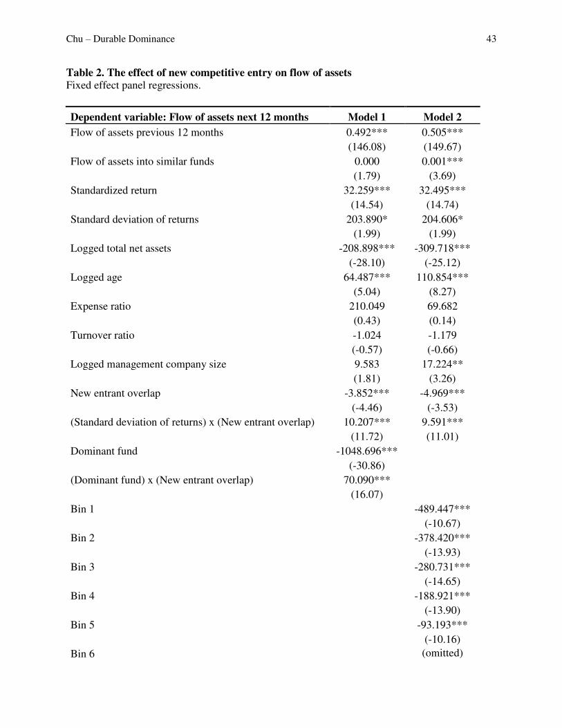
shown in Model 1 of Table 29. As predicted by the proposed theory, the coefficient of the

interaction term was significant and positive. Expected asset flow over the next 12 months

decreased by $3.8 million for each unit increase in new entrant overlap for non-dominant funds.

Dominant funds, on the other hand, benefited from increased competitive entry. Expected asset

9 Including the lagged dependent variable on the right side of the fixed effect panel regression equation can lead to inconsistent and biased results. These errors should not substantively affect the reported results, however, given the current study’s observed levels of residual autocorrelation and the large number of time periods. Additionally, estimates of the effects of non-lagged dependent variables will be biased downwards (Keele and Kelly, 2006), so the reported significant effects are, if anything, under-estimated. In any case, alternative analyses using Arellano-Bond difference and system GMMs also supported the hypothesis.


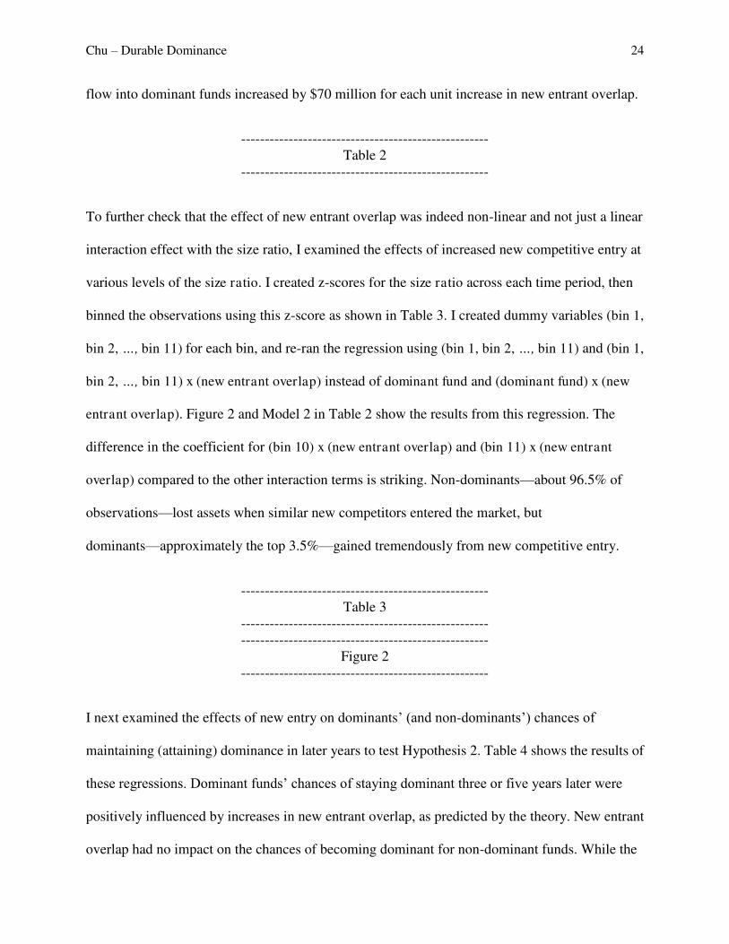
flow into dominant funds increased by $70 million for each unit increase in new entrant overlap.

---------------------------------------------------- Table 2

----------------------------------------------------

To further check that the effect of new entrant overlap was indeed non-linear and not just a linear

interaction effect with the size ratio, I examined the effects of increased new competitive entry at

various levels of the size ratio. I created z-scores for the size ratio across each time period, then

binned the observations using this z-score as shown in Table 3. I created dummy variables (bin 1,

bin 2, …, bin 11) for each bin, and re-ran the regression using (bin 1, bin 2, …, bin 11) and (bin 1,

bin 2, …, bin 11) x (new entrant overlap) instead of dominant fund and (dominant fund) x (new

entrant overlap). Figure 2 and Model 2 in Table 2 show the results from this regression. The

difference in the coefficient for (bin 10) x (new entrant overlap) and (bin 11) x (new entrant

overlap) compared to the other interaction terms is striking. Non-dominants—about 96.5% of

observations—lost assets when similar new competitors entered the market, but

dominants—approximately the top 3.5%—gained tremendously from new competitive entry.

---------------------------------------------------- Table 3

---------------------------------------------------- ----------------------------------------------------

Figure 2 ----------------------------------------------------

I next examined the effects of new entry on dominants’ (and non-dominants’) chances of

maintaining (attaining) dominance in later years to test Hypothesis 2. Table 4 shows the results of

these regressions. Dominant funds’ chances of staying dominant three or five years later were

positively influenced by increases in new entrant overlap, as predicted by the theory. New entrant

overlap had no impact on the chances of becoming dominant for non-dominant funds. While the


focal fund’s size ratio significantly predicted the probability of being dominant up to five years

into the future, currently being dominant was only consequential in determining whether the fund

was dominant the following year.

---------------------------------------------------- Table 4

----------------------------------------------------

These results support the predictions of the proposed theory. Increased entry of similar funds

decreased non-dominant incumbents’ future flows of assets, but increased dominants’ future flows.

Increased competitive entry also increased the probability of dominant funds maintaining

dominance for three or more years. On the other hand, in the absence of new competitive entry, a

fund’s current dominance significantly predicted continued dominance only in the following year.

In sum, increased entry disadvantaged non-dominant incumbents, but benefited and entrenched

dominants.

Robustness checks

A series of robustness checks (some already done, others in progress) provide additional support

for these results. The effects described above are robust to defining competitors in different ways.

Exploratory regressions using CRSP segment codes instead of overlap measures yielded

substantially similar results to those seen in Model 2. CRSP segment codes are used

inconsistently over the years, however, and so I am currently coding social network community

detection algorithms to divide funds into communities. Funds will be considered linked if their

cosine similarity is greater than zero, and the strength of the link defined as the cosine similarity

between the funds. The size ratio is redefined as the ratio of the focal fund’s total net assets to the

average of all other funds in the community, and I will repeat the regressions using this alternate


measure.

Using different definitions of new entry does not substantively change the results. The definition

above counts a fund as a new entrant only if it is a newly-formed fund. An existing fund may

also come into competition with a focal fund when either fund changes its portfolio composition

to be more similar to the other. To examine effects of overall competition increase, I replaced

new entrant overlap with change in competitive overlap in the regression models. Competitive

overlap is calculated for each fund at each time period as the sum of pair-wise cosine similarities

for the focal fund across all other funds existing in the time period (and not just new entrants).

Change in competitive overlap is the net difference between the current value of competitive

overlap and the value 12 months prior.

Regressions using data from 1980 to 1998 yielded the same substantive results for the

independent variables of interest. This is in contrast to Wahal and Wang’s (2011) findings, which

showed no effects of competitive entry on incumbent fund flows before 1998. One possible

reason for their null result is that they were averaging across dominants and non-dominants. The

mutual fund industry grew tremendously from 1980 to 1998. The large number of new entrants

may have resulted (by the mechanisms proposed in this paper) in greatly increased flow to

dominants that offset any decrease in flows to non-dominants, resulting in an average effect that

was not significant. Another possible reason for their null result is that they did not control for

total flows into similar funds. A rising tide may have lifted all boats.

An additional set of regressions tests a hypothesis about the mechanism underlying the observed

main effects:

Hypothesis 3. The effects of new competitive entry on incumbent flows will be mediated


by shifts in the competitive intensity curve, wherein increased new entrant overlap will

lead to a reverse-U shaped increase in the number of similar competitors.

The highest and lowest size ratio funds are predicted to have lower increases in the number of

similar competitors compared to the middle-size ratio funds. I will examine the competitive

intensity curve, and conduct a mediation analysis to see if change in the competitive intensity

curve explains the non-linear relationship between new entrant overlap and future fund flows.

A final set of alternate regressions will attempt to rule out several possible sources of

endogeneity10. One possible alternative explanation for the observed results is that the success of

dominants triggered new entry. Another is that a third factor influenced both new entry in the

current year and disproportionate dominant growth in the following. For example, entrepreneurs

may have recognized that a particular segment was set to grow the next year and founded many

new funds in the segment, but dominants may have benefited disproportionately from increased

investment influx because of their previous investments in scale11. As a first test, I will regress

new entrant overlap in the next year against dominants’ flow of assets previous twelve months to

see if the first alternative explanation holds water. To better rule out more of both types of

alternative explanations, I will use an instrumental variables approach. The number of new

entrants should be correlated with barriers to entry and expected gains from entry. To proxy the

size of barriers and short-term gains from entry, I use average expense fees (expense ratio times

total net assets) accrued during the first three years of fund existence for similar new funds as

my instrument. This measure should not be directly correlated with established fund growth.

Last but not least, I will try to understand the processes underlying the observed regression

10 Including the lagged dependent variable in the regression models already controls for some types of endogeneity. 11 This alternative explanation does not fully explain why near-dominants did not also benefit, however.


results through descriptive explorations of the data. These explorations will look at distributions

and trajectories. I will attempt to confirm that the size distribution of funds within segments is

highly-skewed, and look at how this distribution evolves over time. I will also examine the

distribution of changes in size within segments. This distribution is expected to become

less-skewed compared to the size distribution as more new entrants enter the segment.

I will also visually inspect the dynamics of mutual funds and segments, using 2-dimensional

representations of the mutual fund market. The cosine similarity matrices can be processed with

multi-dimensional scaling techniques or network layout algorithms to create a 2-dimensional plot

of the mutual fund market, with similar funds clustered together (see Appendix 1). This allows a

visual representation of the industry, which can be overlaid with information on community

structure, fund size and dominance. A longitudinal series of maps shows the evolution of

segments and the rise, fall, or continued dominance of funds within segments.

DISCUSSION

Economics, strategy, and sociology have been tremendously successful at generating theories

explaining dominant entrenchment based on exclusion, collusion, and monopolization. This

study is a first attempt at developing and validating theory that explains durable

dominance—dominant entrenchment in the face of mass entrepreneurial entry and decreased

advantages of scale in settings where resources are abundant and widely-available. The proposed

theory suggests that dominants can maintain distinction—competitive advantage—in a world

with no distinctive, monopolizable resources. Durable dominants distinguish themselves by

magnitude rather than exclusivity; more of each resource, not different resources. Elite prep

school students, for example, no longer pride themselves on their access to highbrow culture, but


rather on being able to enjoy a large range of cultural experiences, the scope of which those from

less privileged backgrounds find difficult to emulate (Khan, 2011). An order of magnitude

difference in resources can lead to qualitative differences in capabilities. Those earning $4

million a year travel in private jets, those earning $400,000 in business class, and $40,000

earners in coach.

Easy transposibility and mobility of resources may act to entrench magnitude-based distinction.

Wealth, which is highly scalable, is also increasingly transposable. For individuals, wealth can

buy the “right” type of cultural distinction, which can then be transposed into lucrative careers

(Rivera, 2012). Companies, too, can transpose wealth into and from other needed resources.

High status law firms generate increased profits by attracting partners from lower-status but high

profit firms. Conversely, lower status but high profit firms purchase status by hiring partners

from high status firms with lower profits (Rider & Tan, 2012). Product companies can readily

purchase scalable resources—manufacturing, marketing, distribution, financing, operations—on

the Internet. If all resources are widely available and easily transposable into others, the only

differentiator is who has more, not who has what.

This line of thought forces a shift in how we think about dominant entrenchment. Rather than

considering dominant tactics of exclusion, collusion, and monopolization, we need to consider

the ecological distribution of resources among competitors and the trajectories of these resource

distributions. The proposed theory predicts that durable dominance is contingent on order of

magnitude differences between dominants’ and non-dominants levels of contested resources.

Given such a highly-skewed distribution of resources, if the non-dominant have no way of

accumulating resources an order of magnitude greater than what they currently possess, they

cannot become dominant—and durable dominance occurs.


Analyzing highly-skewed distributions requires separating the analysis of dominants from that of

non-dominants. The “1%” are different from the rest, but averaging or taking the median over

the population obfuscates these differences. Gathering data on dominants often presents an

empirical difficulty, however. Data on the richest Americans, for example, are rarely available in

general social surveys. Nonetheless, this study—along with the related studies in my

dissertation—shows that gathering and analyzing data on highly-skewed distributions is possible,

and necessary to understand durable dominance.

The policy implications of the proposed theory are straightforward but counterintuitive.

Dominants may benefit from a strategy of opening their markets to new entrants and fostering

small competitors. These upstarts will weaken potential challenges to the dominants’ dominance

from large but non-dominant incumbents. Whether guided by altruism or cunning, this seems

precisely the strategy that Google, for example, is executing when it routinely provides funding,

employees, technology, and platform access to startups. An elite business school worried about

losing its elite status could conceivably attempt to entrench its position by investing resources in

democratizing massive open online course (MOOC) creation and distribution. Giving away

access to world-class production and distribution technologies to even small colleges could flood

the marketplace with new entrants, force other schools immediately below elite status to invest

resources in developing their own MOOC capabilities, and ultimately entrench the hypothetical

protagonist’s elite position.

Policy-makers and non-dominants face a more difficult choice. The proposed theory suggests

that currently taken-for-granted measures for loosening dominants’ hold on contested resources

may backfire—unless the measures are executed in tandem with reductions in dominants’ vastly

disproportionate resources to levels near their competitors’ averages. Durable dominance may be


a natural and inevitable consequence of an open society (such as today’s United States) where

wealth is unlimited and eminently transposable, and competition is revered.


APPENDIX 1. COSINE SIMILARITY

Funds are represented as vectors in stock space, and cosine similarity is defined as the cosine of

the angle between two funds. In the simple two-stock example pictured in Figure A1, Fund 1

holds $5 million in Stock A and $0 in Stock B, and is represented by the vector (5, 0). Fund 2

holds $2 million in Stock B and none in Stock A. Fund 3 holds $2 million in stock A and $1

million in stock B. The cosine similarities for fund pairs 1-2, 1-3, and 2-3 respectively are 0,

2/√ , and 1/√ . Similarity values are calculated numerically using the vector inner product:

cos(XY) = | || |.

---------------------------------------------------- Figure A1

----------------------------------------------------

The actual stock space is high-dimensional, with as many dimensions as distinct domestic stocks

held by mutual funds. Multi-dimensional scaling or network layout techniques allow us to

project this space onto a 2- or 3-dimensional map. The nodes in this map are mutual funds, and

similar (in portfolio composition) mutual funds will be clustered together in the map. This map

can then be used to explore the structure of the mutual fund market and its evolution over time

(Figure A2).

---------------------------------------------------- Figure A2

----------------------------------------------------

The models proposed in this paper suggest that the identity of dominants will sometimes change

when the number of funds in a segment is still small, but that the dominant fund at the time of an

explosion in the number of funds in the segment will remain dominant for a long time thereafter.


This intuition can be explored visually, as in Figure A2A.

The cosine similarity measure may be useful for other research studies. The mutual fund

similarity and mapping data is of obvious interest to scholars interested in the industry evolution

of mutual funds. The data can show the creation and growth of new fund types, movement of

groups of funds in stock space, and movement of funds between groups (see Figure A2B). The

dataset may also be of use to researchers studying categories and network communities.


REFERENCES

Bain, J. S. 1968. Industrial organization (2nd ed.). New York: Wiley.

Barney, J. 1986. Strategic factor markets: Expectations, luck and business strategy. Management

Science, 32: 1231–1241.

Barney, J. 1991. Firm resources and sustained competitive advantage. Journal of Management, 17: 99–120.

Bogle, J. C. 2003. Mutual fund industry practices and their effect on individual investors. Statement before the U.S. House of Representatives, Subcommittee on Capital Markets, Insurance, and Government Sponsored Enterprises of the Committee on Financial Services (Mar. 12, 2003). Downloaded from https://personal.vanguard.com/bogle_site/sp20030312a.html.

Bourdieu, P. 1984. Distinction: A social critique of the judgement of taste. Cambridge, MA: Harvard University Press.

Caves, R. E., & Porter, M. E. 1977. From entry barriers to mobility barriers: Conjectural decisions and contrived deterrence to new competition. Quarterly Journal of Economics,

91: 241–262.

Christensen, C. M., & Bower, J. L. 1996. Customer power, strategic investment, and the failure of leading firms. Strategic Management Journal, 17: 197–218.

Christensen, C.M. 1997. The innovator’s dilemma: When new technologies cause great firms to fail. Boston: Harvard Business School Press.

Chu, J. S. G., & Davis, G. F. 2013. Who killed the inner circle? The collapse of the American

corporate interlock network. Working paper, University of Michigan, Ann Arbor, MI. Available at http://ssrn.com/abstract=2061113.

Coates, J. C., & Hubbard, R. G. 2007. Competition in the mutual fund industry: Evidence and implications for policy. Journal of Corporation Law, 33: 151–222.

Cool, K., Costa, L. A., & Dierickx, I. 2002. Constructing competitive advantage. In A. Pettigrew, H. Thomas, & R. Whittington (Eds.), Handbook of strategy and management: 55–71. London: Sage.

Davis, G. F. 2013. After the corporation. Politics & Society, 41: 283–308.

Demsetz, H. 1973. Industry structure, market rivalry, and public policy. Journal of Law and

Economics, 16: 1–9.

Dierickx, I., & Cool, K. 1989. Asset stock accumulation and sustainability of competitive advantage. Management Science, 35: 1504–1511.

DiMaggio, P., & Mohr, J. 1985. Cultural capital, educational attainment, and marital selection. American Journal of Sociology, 90: 1231–1261.

Domhoff, G. W. 1967. Who rules America? Englewood Cliffs, NJ: Prentice-Hall.


Domhoff, G. W. 1970. The higher circles. New York: Vintage.

Fisher, F. M. 1979. Diagnosing monopoly. Quarterly Review of Economics and Business, 7: 671–697.

Freeman, J. P., & Brown, S. L. 2001. Mutual fund advisory fees: The cost of conflicts of interest. Journal of Corporation Law, 26: 610–673.

Gibrat, R. 1931. Les inegalites economiques. Paris: Librairie du Recueil Sirey.

Hunt, M. 1972. Competition in the major home appliance industry, 1960-1970. Ph.D. dissertation, Harvard University, Cambridge, MA.

Katz, M. L., & Shapiro, C. 1992. Product introduction with network externalities. Journal of

Industrial Economics, 40: 55–83.

Keele, L., & Kelly, N. J. 2006. Dynamic models for dynamic theories: The ins and outs of lagged dependent variables. Political Analysis, 14: 186–205.

Khan, S. R. 2011. Privilege: The making of an adolescent elite at St. Paul's school. Princeton, NJ: Princeton University Press.

Khan, S. R. 2012. The sociology of elites. Annual Review of Sociology, 38: 361–377.

Khorana, A., & Servaes, H. 2012. What drives market share in the mutual fund industry?. Review of Finance, 16: 81–113.

Kopczuk, W., Saez, E., & Song, J. 2010. Earnings inequality and mobility in the United States: Evidence from Social Security data since 1937. The Quarterly Journal of

Economics, 125: 91–128.

Lamont, M. 1992. Money, morals, and manners: The culture of the French and American

upper-middle class. Chicago: University of Chicago Press.

Levine, L. W. 1990. Highbrow/lowbrow: The emergence of cultural hierarchy in America. Cambridge, MA: Harvard University Press.

Lippman, S. A., & Rumelt, R. P. 1982. Uncertain imitability: An analysis of interfirm differences in efficiency under competition. The Bell Journal of Economics, 13: 418–438.

Mason, E. S. 1939. Price and production policies of large scale enterprises. American Economic

Review, 29: 61–74.

Merton, R. K. 1968. The Matthew effect in science. Science, 159: 56–63.

Michels, R. [1911] 1962. Political parties: A sociological study of the oligarchical tendencies

of modern democracy. New York: Free Press.

Miliband, R. 1969. The state in capitalist society. New York: Basic.

Mills, C. W. 1956. The power elite. New York: Oxford University Press.

Mizruchi, M. S. 1992. The structure of corporate political action. Cambridge, MA: Harvard University Press.


Mizruchi, M. S. 2013. The fracturing of the American corporate elite. Cambridge, MA: Harvard University Press.

Mosca, G. [1896] 1939. The ruling class: Elementi di scienza politica. New York: McGraw-Hill.

Penrose, E. 1959. The theory of the growth of the firm. London: Basil Blackwell.

Peterson, R. A., & Kern, R. M. 1996. Changing highbrow taste: From snob to omnivore. American Sociological Review, 61: 900–907.

Pfeffer, J. 1995. Mortality, reproducibility, and the persistence of styles of theory. Organization

Science, 6: 681–686.

Piketty, T., & Saez, E. 2003. Income inequality in the United States, 1913-1998. Quarterly

Journal of Economics, 118: 1–39.

Porter, M. E. 1980. Competitive strategy: Techniques for analyzing industries and competitors. New York: Free Press.

Reed, R., & DeFillippi, R. J. 1990. Causal ambiguity, barriers to imitation, and sustainable competitive advantage. Academy of Management Review, 15: 88–102.

Rider, C. I., & Tan, D. 2012. Labor markets as status markets: Organizational trade-offs

between status and profitability. Working paper, Emory University, Atlanta, GA.

Rivera, L. A. 2012. Hiring as cultural matching: The case of elite professional service firms. American Sociological Review, 77: 999–1022.

Samuelson, P. A. 1947. Foundations of economic analysis. Cambridge, MA: Harvard University Press.

Schmalensee, R. 1989. Inter-industry studies of structure and performance. In R. Schmalensee & R. Willig (Eds.), Handbook of industrial organization, vol. 2: 951–1009. Amsterdam: North-Holland.

Schoonhoven, C. B., Meyer, A. D., & Walsh, J. P. 2005. Pushing back the frontiers of organization science. Organization Science, 16: 453–455.

Schumpeter, J. [1942] 1994. Capitalism, socialism, and democracy. London: Routledge.

Sirri, E. R., & Tufano, P. 1998. Costly search and mutual fund flows. Journal of Finance, 53: 1589–1622.

Spitzer, E. 2004. Testimony before the United States Senate Governmental Affairs Committee, Subcommittee on Financial Management, the Budget and International Security (Jan. 27, 2004). Downloaded from http://www.gpo.gov/fdsys/pkg/CHRG-108shrg92686/html/CHRG-108shrg92686.htm.

Stigler, G. J. 1968. The organization of industry. Chicago: University of Chicago Press.

Sutton, J. 1991. Sunk costs and market structure: Price competition, advertising, and the

evolution of competition. Cambridge, MA: MIT Press.


Swensen, D. F. 2005. Unconventional success: A fundamental approach to personal

investment. New York: Free Press.

Tilly, C. 1998. Durable inequality. Berkeley: University of California Press.

Useem, M. 1984. The inner circle: Large corporations and the rise of business political activity

in the US and UK. New York: Oxford University Press.

Wahal, S., & Wang, A. Y. 2011. Competition among mutual funds. Journal of Financial

Economics, 99: 40–59.

Wernerfelt, B. 1984. A resource-based view of the firm. Strategic Management Journal, 5: 171–180.


FIGURES AND TABLES

Figure 1. Revenue distributions (competitive intensity curve)

A (left). With Matthew effect and no entry. Stylized illustration of highly-skewed (power law)

revenue distributions in a market with no exit or entry, and rich-get-richer dynamics. Companies

with higher revenue levels have fewer competitors with similar revenues.

B (right). With Matthew effect and mass entry. Competitive intensity curve (solid line) after

market is opened to entry. Mass entry of new competitors flattens the competitive intensity curve

for those below a threshold, increasing competitive intensity by several orders of magnitude for

firms slightly below the threshold. In the case depicted below, the number of similar competitors

for an incumbent with revenue level Rt increases by almost two orders of magnitude.

log(n)

n = # of

actors

with

revenue

level R

log(R). R = revenue level

Mobility

No

mobility

Mobility

Rt

log(R). R = revenue level


Figure 2. The non-linear effect of new competitive entry on flow of assets

Bars and left axis indicate the predicted effect of a unit increase in new entrant overlap on the focal fund’s flow in the next 12 months. Line and right axis show the percentage of fund-quarter observations within each size ratio bin. See Table 3 and article text for details of the binning.

-3%

0%

3%

6%

9%

12%

15%

18%

21%

-10

0

10

20

30

40

50

60

70

1 2 3 4 5 6 7 8 9 10 11

% o

f o

bse

rva

tio

ns

b(n

ew

en

tra

nt

ov

erl

ap

)

Binned size ratio


Figure A1. A simple two-stock cosine similarity example

Cosine similarity is defined as the cosine of the angle between two funds, when the funds are represented as vectors in stock space.

cos θ = √5

cos θ = 0

cos θ = √5

Stock B

Stock A

Fund 2: (0, 2)

Fund 3: (2, 1)

Fund 1: (5, 0)


Figure A2. Mutual fund structure maps (mockups)

The nodes in the map are mutual funds, and funds with similar stock holdings are placed closer

together on the map.

A. Dominant change within a community. The red dot represents the dominant fund at Time 1.

By Time 2, the yellow dot fund has become dominant, but is replaced by Time 3 by the black dot

fund. The community grows rapidly from Time 3 to Time 5, and the black dot fund maintains its

dominance throughout this growth.

B. Mutual fund industry evolution. Five distinct communities (including one isolate) exist at

Time 1. By time 2: New entrants have increased the number of funds in the top-left community,

while fund exits have decreased the size of the top-right community. The bottom-left community

has broken apart into two communities. Several funds from the central community have joined

the isolate on the bottom right.


Table 1. Data descriptions

Variable Description

Flow of assets next 12

months

The net flow of investments into the focal fund over the next 12 months,

calculated as the net growth in fund assets beyond reinvested dividends

and asset influx from mergers (cf. Sirri and Tufano, 1998). Flows for

four quarters were summed to create twelve month trailing measures.

Dominant in year+ n A dichotomous variable that equals 1 if Dominant fund in year+n, where

n = 1, 2, 4, 5. See below for definition of Dominant fund.

Flow of assets

previous 12 months

The net flow of investments into the focal fund over the previous 12

months. See Flow of assets next 12 months above for measure details.

Flow of assets into

similar funds

Cosine similarity-weighted average of flows into similar funds. Flow

into the focal fund is included in the sum.

Standardized return The focal fund’s z-score (across all funds present in each time period) of

12-month fund returns from CRSP.

Standard deviation of

returns

The standard deviation of the focal fund’s past 12 months’ monthly returns from CRSP.

Logged total net

assets

The base 10 log of the total net assets of the fund from CRSP.

Logged age The base 10 log of the age of the fund in months from CRSP.

Expense ratio The fund’s expense ratio from CRSP.

Turnover ratio The fund’s turnover ratio from CRSP.

Logged management

company size

The base 10 log of the total net assets of the fund’s management company. The management company code from the Thomson database

was used to determine a fund’s management company.

New entrant overlap The sum of pair-wise cosine similarities for the focal fund across all new

entrants.

Size ratio The ratio of the focal fund’s total net assets to the cosine similarity-weighted average of its competitors’ total net assets.

Dominant fund A dichotomous variable that equals 1 when the focal fund’s size ratio is

greater than ten. Dominant fund = 1 for 1,212 observations (1.04% of

total observations). Seventy-six funds are dominant in one or more time

periods. I also use the z-score of the size ratio across contemporary

funds as an alternate measure of dominance.


Table 2. The effect of new competitive entry on flow of assets

Fixed effect panel regressions.

Dependent variable: Flow of assets next 12 months Model 1 Model 2

Flow of assets previous 12 months 0.492*** 0.505***

(146.08) (149.67)

Flow of assets into similar funds 0.000 0.001***

(1.79) (3.69)

Standardized return 32.259*** 32.495***

(14.54) (14.74)

Standard deviation of returns 203.890* 204.606*

(1.99) (1.99)

Logged total net assets -208.898*** -309.718***

(-28.10) (-25.12)

Logged age 64.487*** 110.854***

(5.04) (8.27)

Expense ratio 210.049 69.682

(0.43) (0.14)

Turnover ratio -1.024 -1.179

(-0.57) (-0.66)

Logged management company size 9.583 17.224**

(1.81) (3.26)

New entrant overlap -3.852*** -4.969***

(-4.46) (-3.53)

(Standard deviation of returns) x (New entrant overlap) 10.207*** 9.591***

(11.72) (11.01)

Dominant fund -1048.696***

(-30.86)

(Dominant fund) x (New entrant overlap) 70.090***

(16.07)

Bin 1 -489.447***

(-10.67)

Bin 2 -378.420***

(-13.93)

Bin 3 -280.731***

(-14.65)

Bin 4 -188.921***

(-13.90)

Bin 5 -93.193***

(-10.16)

Bin 6 (omitted)


Bin 7 66.418***

(7.53)

Bin 8 65.410***

(5.19)

Bin 9

-88.697***

(-4.90)

Bin 10

-518.626***

(-18.69)

Bin 11 -1501.781***

(-32.13)

(Bin 1) x (New entrant overlap) 5.207

(0.27)

(Bin 2) x (New entrant overlap) -2.634

(-0.38)


(-0.38)


(0.15)


(-0.01)

(Bin 6) x (New entrant overlap) (omitted)


(0.46)


(0.40)


(1.64)

(Bin 10) x (New entrant overlap) 25.645***

(7.27)

(Bin 11) x (New entrant overlap) 72.114***

(15.26)

Constant 333.164*** 511.850***

(11.18) (15.57)


Table 3. Binning based on standardized size ratios

Bin

number Z-score range

% of

observations

1 < -2.25 1.52%

2 -1.75 - -2.25 3.00%

3 -1.25 - -1.75 6.41%

4 -0.75 - -1.25 11.70%

5 -0.25 - -0.75 16.30%

6 -0.25 - 0.25 18.93%

7 0.25 - 0.75 17.94%

8 0.75 - 1.25 14.35%

9 1.25 - 1.75 6.37%

10 1.75 - 2.25 2.19%

11 > 2.25 1.29%


Table 4. Effect of new competitive entry on log-odds of being dominant in n years

Fixed effect panel logit.

Dependent variable: Dominant in

year+n Year + 1 Year + 2 Year +3 Year + 5

Flow of assets previous 12 months 0.000* 0.000*** 0.000* -0.000

(2.50) (3.52) (2.36) (-0.47)

Flow of assets into similar funds 0.000* 0.000*** 0.000*** 0.000***

(2.01) (4.55) (4.14) (7.85)

Standardized return 0.332** 0.411*** 0.375*** 0.528***

(3.23) (3.91) (3.56) (3.51)

Standard deviation of returns -4.573 -19.837*** -22.034*** 13.269*

(-1.20) (-4.53) (-4.74) (2.09)

Logged total net assets 2.471*** 1.873*** 0.307 -4.850***

(4.51) (3.79) (0.66) (-6.05)

Logged age -7.524*** -8.965*** -10.225*** -7.792***

(-6.89) (-7.69) (-8.30) (-4.42)

Expense ratio 57.236 250.625** 209.917* 395.607**

(0.61) (2.63) (2.18) (2.81)

Turnover ratio -0.536 -0.351 -0.351 -0.845

(-1.59) (-0.96) (-0.92) (-1.57)

Logged management company size -0.728* -0.723* -1.015** -2.623***

(-2.03) (-2.02) (-2.78) (-5.11)

New entrant overlap -0.007 0.026 -0.029 -0.042

(-0.26) (0.77) (-0.93) (-1.05)

Size ratio 0.046* 0.033* 0.034* 0.067**

(2.49) (2.07) (2.20) (2.91)

Dominant fund 1.311*** 0.206 -0.047 -0.060

(6.82) (1.00) (-0.22) (-0.18)

(Dominant fund) x (New entrant overlap) -0.012 0.034 0.114** 0.264***

(-0.44) (0.81) (2.75) (4.97)

Date post:	19-Aug-2018
Category:	Documents
Upload:	lykiet
View:	217 times
Download:	0 times

Durable Dominance: Dominant Entrenchment through...

Documents