336
• • •

Durham E-Theses
Surface composition pro�les in some polymer mixtures
Hopkins, Ian
How to cite:
Hopkins, Ian (1994) Surface composition pro�les in some polymer mixtures, Durham theses, DurhamUniversity. Available at Durham E-Theses Online: http://etheses.dur.ac.uk/5518/
Use policy
The full-text may be used and/or reproduced, and given to third parties in any format or medium, without prior permission orcharge, for personal research or study, educational, or not-for-pro�t purposes provided that:
• a full bibliographic reference is made to the original source
• a link is made to the metadata record in Durham E-Theses
• the full-text is not changed in any way
The full-text must not be sold in any format or medium without the formal permission of the copyright holders.
Please consult the full Durham E-Theses policy for further details.
Academic Support O�ce, Durham University, University O�ce, Old Elvet, Durham DH1 3HPe-mail: [email protected] Tel: +44 0191 334 6107
http://etheses.dur.ac.uk

The copyright of this thesis rests with the author.
No quotation from it should be published without
his prior written consent and information derived
from it should be acknowledged.
October li994
lian Hopkinson
University of Dll.llrlham
Supervisor
Randal W. Richards
University of Durham
A thesis submitted to the University of Durham in partial fulfilment of the
regulations for the Degree of Doctor of Philosophy
~ (R) r\-'j n !,\) f'l'\~~'? U cJ .... l .~ .. J

Surface ComJPOSfitfiollll. !Profnlles n1111. §orne IPoDymer Miduures
][~un l!-noJPlknll1son
!Ph[) Tlhlesis Octolber R994
Albstrad
The surface composition of selected polymer mixtures has been studied to a
depth of circa 4000A with a resolution of up to lOA using neutron reflectometry (NR)
and nuclear reaction analysis (NRA). The effective interaction parameters, x, of several
blends have been measured as a function of both composition and temperature, using
Small Angle Neutron Scattering (SANS) and the incompressible random phase
approximation, in order to understand the surface segregation behaviour of the polymer
blends. No surface segregation was observed in annealed blends of syndiotactic poly
(methyl methacrylate) (h-PMMA) with perdeuterated poly (methyl methylacrylate) (d
PMMA), where the h-PMMA was the majority component with a high molecular weight
and the d-PMMA had lower molecular weights. Values of X for these blends showed a
chain length disparity effect, higher disparity led to a small negative X· Increases in X
were observed at low volume fractions of d-PMMA. Surface segregation of
perdeuterated poly (ethylene oxide) (d-PEO) to the polymer - silicon oxide interface of
an annealed d-PEO/h-PMMA blend was observed, where the bulk volume fraction of the
d-PEO was <0.30. The surface composition profile could not be described by current
theory. Measured X values were small and negative and there was a change in X on
changing the locus of deuteration from PEO to PMMA in a PEO!PMMA blend. These
blends exhibited a decrease in X at low volume fractions of PEO. Polymer brushes were
found at the air - polymer interface of a blend of low molecular weight polystyrene (h
PS) with perdeuterated polystyrene with a single perfluorohexane end group (d-PS(F))
or two perfluorohexane end groups (d-PS(F2)). These results were in good agreement
with a self consistent field theory. Similar blends of high molecular h-PS I d-PS(F)
showed enhanced surface segregation, compared to blends with no perfluorohexane end
groups. NR data showed that the surface of a blend of polystyrene with perdeuterated
dibutyl phthalate (d-DBP) (a model additive) was enriched with d-DBP over a 30A
length scale. The loss of d-DBP from a thin film(- 800A thick) was observed using NR
and attenuated total reflection (ATR) infra red spectroscopy.

AckrrwwHed.gemeHllts
I am grateful to Randal Richards for his persistent and enthusiastic supervision
and for tolerating my scepticism of anything he said even though he was nearly always
right! I'd also like to thank Prof. W.J. Feast our leader, for making the IRC a good place
to work.
A number of people at the IRC in Polymer Science have been directly involved in
this work and I'd like to thank: F.T. Kiff who has synthesised all the polymers I have
used, with a degree of competence I could only dream of emulating. Gordon 'Backup'
Forrest who was responsible for the size exclusion chromatography and J. Say and Dr A.
Kenwright who ran and helped in the analysis of n.m.r spectra. I am also grateful to the
Mechanical Workshop, who have made various oddly shaped bits of metal for me and
the Glassblowers.
I have had the pleasure of working with a number of instrument scientists, these
are: Dr J. Penfold, Dr J. Webster and Dr D. Bucknall (on CRISP at the Rutherford
Appleton Laboratory), Dr S. King and Dr. R. Heenan (on LOQ at the Rutherford
Appleton Laboratory) and Dr A. Clough ( nuclear reaction analysis at Surrey
University), these people have all put up with my incessant questions and have made
useful suggestions in the analysis of data, thanks are also due here to Dr D. Sivia, also at
Rutherford Appleton Laboratory for allowing me to use his neutron reflectivity data
analysis programs.
I'd like to thank Prof. K.R. Shull for allowing me to use LAYERS, his self
consistent field theory program and also for useful discussions.
I have enjoyed many stimulating meetings with my collaborators at Strathclyde
University (Prof. R.A. Pethrick, DrS. Affrossman, M. Hartshorne (also responsible for
the synthesis of perdeuterated dibutyl phthalate)) and at Courtaulds Plc ( Dr H. Munro,
Dr T. Farren, S. Wills, Dr J. Connell). I would like to thank Courtaulds Plc and SERC
for funding this work.
The IRC has been a fun place to work and I'd like to mention specifically my
immediate cohort: Norman 'Sleepwalker' Clough, Neil 'Red shoes' Stainton, Don
'whoops' Davison and Cecilia 'Disk full' Backson and some distinguished others 'Red'
Lian Hutchings, Stella 'Sainsbury's' Gissing, Dave 'The Viking' Parker, Pangiotis 'PD'
Dounis, all otl1er members of the IRC are mentioned implicitly.
Finally I'd like to thank Sharon who has kept me relatively sane over the last
thi-ee years, and has put up with my occasional sanity lapses during writing up and my
parents who haven't seen me very often recently (my fault!).


Abstract
Acknowledgements
Contents
Declaration
~. ~ ~ntll'((»dl!.fl~~o((»!rn
~. ~. SUioiaces
~.2. SUioia~ce All1la~ysos TecrrmnqiUies
~.3. Ove~rvoew oi ~his work
~.4. Reiell'ell1lces foil' Sectio01 1
2. Theory
2.1. Polymer~po~ymell' 'i:hell'modynamocs
2.2. SUirface enll'nchmell1li ~heory
2.3. Polymer !brush ftheowy 2.3.1. SCJF tlheory 2.3.2. §calling 'Jl'lhleory
2.4. IReierences foil' Seciion 2
3. Te c tn11rn u qpUI es
3.1. NeUJ'i:ron TechniqiUies 3.1.1. Small Angle Neutron Scattering 3.1.2. Neutron IR.eflectometry
3.2. Nuclear Reaction Analysis
3.3. Attenuated Total Reflection Spec'i:roscopy
3.4. References foil' Section 3
4. Expe1r8menta~
4.1. Materials ~.1.1. Synthesis 4lJ .. 2. MonecuRar weights arnd distrilbutions 4.1.3. Tadicity
4.2. Smal~ Angle Neutroll1l Scattering 4.2.11. §ample IPreiParatimn 41.2.2. JLOQ 41.2.3. Calibration 41.2.41. lBackgrmmd subtraction 41.2.5. lData analysis metillods
~
~
7
~0
13
16
15
26
34 34! ~3
47
5()
50 52 55
64
67
71
73
73 73 76 78
79 79 79 S.D. 87 88

4.3. INiell.n~D'OI11l Reff!ectomeftll'y 41.3.1. SampH~ jpreparatnollll 41.3.2. CliU§IP 41.3.3. Data arnalysns metlhods
~.4. INUJc~ea~ IReacftooiTU Ana~ysus
~.5. Aftfte1111l.naiieo1 Toia~ IRe~~ectioiTU spectroscopy
4.5. IRe~ell'ernces ~or SecUol11l 4
90 90 91 97
1100
102
105
5. Pe~rdleu.n~ell'a~edl !PJ©~y (me~hy~ m~~hacqJ~tal~~) I [p(Q)~y (meUily~ me~1nltal~Ulf~tal~~) IMelllldls ~ (Q)1
5.~. T~e1Tmodly111amncs 107 5.1.n. Experimentan 107 5.n.z. Results 109 5.ll.3. Discussion 123 5.1.41. Conclusions 132 5.:n..s. References for Section §.1 133
5.2. Su1r~ace euuictnment 135 5.2.1. Experimental ll35 5.2.2. Resll.llDts 138 5.2.3. Discussion 147 §.2.41. Conclusions 153 5.2.§. References for Section 5.2 154
6. P©~Y (etlhrif~ene oxudle) I po~y (mei'hy~ metha~ryh:~te) lbl~ell'ildls ~56
5.1. Thermodynamics 155 6.1.1. ExperimentaB 156 6.ll.2. ResuBts 157 6.L3. Discussion 171 6.1.4. Conclusions 178 6.1.§. References for Section 6.1 179
6.2. Surface enrichment 181 6.2.1. Experimental 181 6.2.2. Results 184 6.2.3. Discussion 198 6.2.4. Conclusions 203 6.2.5. References for Section 6.2 204
7. End cappedlperdeuteratecdl polystyrene I po~ystyrene blends 206
7.1. Experimental 205
7.2. !Results 212
7.3. Discussion 242
7.4. Co111ch.JJsions 259

7.5. 1Reiell'ell1lces ioll' Section 7 260
8. IP\~Il'dlelUitell'a~~e<dl <dlilbiU~Y~ p~~~a.~a~~e I jp)COJ~ys~yll'enJe lb~emdls 262
8.~. Expewimenta! 262
8.2. IResu.nlts 264
8.3. IDliS<CUSSDIOII1 283
8.4. Conc!fi.nsicms 294
8.5. Re1ell'el!1lces ~ow Sectioll1l 8 295
9. (C(Qlll1te~ll.DSDtOirnS a111dl IFlUlrthlell' W!Olll'il{ 296
~OJ. Ap1Pell1dlices 298
1 !0.1. G!ossawy o~ symroo!s 298
10.2. Adlo1itionai data 306
10.3. Pulbiocations, lec~u.ues and Conferences AUell1lded 308
10.4. Computer programs 315

All work contained within this thesis is my own work, unless stated otherwise, and
has not previously been submitted for any other qualification.

1. 1 Surfaces
The arm of this work was to study and understand the smface segregation
behaviour of polymer - polymer blends and a polymer - 'additive' system. The reason
for this interest is that the surface composition of a polymer mixture influences properties
of the mixture. In blends this includes wettability, adhesion, solvent penetration and
weathering. For 'additives' the interest will be in whether certain additives accumulate
preferentially at the smface, in some situations this will be desirable such as when the
additive is used to lubricate the polymer during processing or alternatively such
segregation could be undesirable because the additive is required to modify the bulk
properties of the blend and hence is at best wasted at the surface. Ultimately the hope is
that by understanding the processes and conditions which influence surface segregation
behaviour it will be possible to control the phenomena to produce industrially useful
properties at lower cost than current methods. However this work is not concerned with
such properties, but rather in the near surface composition profile from which the
prope1ties ultimately stem.
Two processes by which the surface composition of a miscible polymer blend can
differ from the bulk composition have been considered. These are surface enrichment
and brush formation, illustrated schematically in Figures 1.1a and 1.1 b. Surface
enrichment is the 'wetting' of the surface of a blend by the component of lower surface
energy, brush formation is driven by end groups on polymers in the blend which will
attach these polymers to an interface.
The study of surface enrichment behaviour in polymer blends has developed
over the past -15 years since the general theoretical work of Calm1, who considered the
smface emichment behaviour of blends in general. This work was followed by
development of a theory specifically for polymer blends by Pincus and Nakanishi2 and
Schmidt and Binder3 . Subsequently these theories have been explored more thoroughly
and in addition Monte Cm·lo4 and Self Consistent Field5 theory models have been
developed.

polymer
lFfigure Lll.a: Schematic of Surface ernrichmernt
air
polymer
Figure Lib: Schematic of brush formation
These theories predict that the variation of volume fraction of the enriching polymer as a
function of depth from the interface occurs over lengths -Rg (where Rg is the radius of
gyration of the enriching polymer). This corresponds typically to distances of the order
-50A to -200A, a typical composition versus depth profile for a blend sustaining surface
enrichment is shown in Figure 1.2. Enrichment may equally occur at the air - polymer or
polymer - substrate interface of a film. The horizontal axis in this figure indicates the
depth, z, from the interface and the vertical axis is the volume fraction, Q>, of the
emiching component. In a binary blend it will be assumed that Q> + (1-Q>) = 1, where (1-
Q>) is the volume fraction of the second component of the blend.
2

-c 0
+-' () 0 .._
'+-
Q)
E :J
0 >
Depth /A
Figure 1.2: Genernc surface enrichment composition versus d!epth profile.
Figure 1.2 also illustrates the definitions of the smface volume fraction, ~air, and the
smface excess, z *, which is given in Equation 1.1. ~B is the bulk volume fraction of the
emiching polymer.
Equation 1.1
The smface analysis techniques that can be used to study near surface structure at the
required length scale will be introduced shortly.
Theories2'3 show that the bulk thennodynamics of the polymer blend are
important in detennining the shape of the near surface composition profile of the
eruiching polymer. When the blend is close to one phase - two phase coexistence the
characteristic decay length of the enrichment profile increases since the free energy cost
of maintaining a region at the smface with a composition different from that in the bulk is
lower closer to the phase boundary. For this reason the bulk thennodyna1nics of the
polymer blends used in this work have been investigated using Small Angle Neutron
Scatteling (SANS) using the theoretical results of de Gennes6, an 'effective' Flory -
3

Huggins interaction parameter is detetmined and hence the thennodynamics of the blend
are revealed in the context of the Flory- Huggins lattice theory of polymer blends7•
Following theoretical predictions there has been an experimental interest in the
surface emichment behaviour of polymer blends. The primary interest, for making
detailed comparisons between theory and experiment, has been in the perdeuterated
polystyrene (d-PS) I polystyrene (h-PS) blend system. It has been found by Bates and
Wignall8 that, rather than being completely ideal such blends of a polymer with its
perdeuterated isomer are characterised by a small positive Flory - Huggins interaction
parameter, XFH, and so at sufficiently high degrees of polymerisation such blends will
exhibit 'upper critical solution temperature' (UCST) phase behaviour, where the one
phase region is found at higher temperatures. Subsequently non-zero values of XFH have
been measured for a range of blends of hydrogenous polymers with their perdeuterated
isomers (see section 5.1.3 for examples). In addition to introducing simple phase
behaviour the deuteration acts as a 'label' for a variety of expe1imental techniques.
The initial work on the surface enrichment behaviour of the d-PS/h-PS blend was
by Jones et at '10 who showed that surface enrichment of the d-PS to the air - polymer
interface occurred in 'symmetric' high molecular weight blends (that is where the
degrees of polymerisation of the hydrogenous, NH, and deuterated, No, components are
approximately equal). The variation of the degree of enrichment as a function of the
bulk volume fraction of d-PS, <J>n, was obtained and from these data it was concluded
that the enrichment was driven by a surface energy difference of 0.078 mJ m-2 in favour
of the deuterated polymer. This difference is small when compared to surface energy
differences that can be measured directly and when compared to the differences in
surface energy typically found between the components of a miscible blend. Because the
high molecular weight of the polymers forces the blend close to the phase boundary tllis
tiny surface energy difference is sufficient to drive ernichment. The work of Jones eta/
culminated in showing that although the surface enrichment behaviour of d-PS/h-PS was
described quite accurately by the theory of Schmidt and Binder, the shape of the near
surface composition profile differed subtly from theoretical prediction. This has been
attributed, at least in part, to the use of the approximation that the surface energy
difference can be assumed to act like a delta function potential at the interface, rather
than acting over a longer range that extends a short distance into the blend.
4

Fmther work by Hariharan et a/11 on d-PSih-PS blends has explored the effect
that a difference in molecular weight between the. d-PS and h-PS has on the surface
enrichment behaviour. Entropy favours lower molecular weight polymers at the surface
and Hruiharan et al were able to force h-PS to the smface of d-PSih-PS blends by
lowering the moleculru· weight of the h-PS to values well below that of the d-PS.
Budkowski et a/12 have shown that in contrast to the work of Jones et al where no
enrichment was observed to the polymer - subsu·ate interface ( the substrate was silicon),
enrichment of d-PS does occur to a silicon surface which retains its native silicon dioxide
layer. The surface energy difference between d-PS and h-PS against silicon dioxide is
rather smaller than that versus air.
In addition to this work on d-PSih-PS there has also been experimental work on
the poly (ethylene oxide) (PEO) I poly (methyl methacrylate) (PMMA)13 and polystyrene
I poly (vinyl methyl ether) (PVME) 14 '15
'16 systems although detailed detenninations of
the near surface composition profile have not been made. There has also been a short
paper on surface enrichment in the perdeuterated PMMA I hydrogenous PMMA blend17
, showing a very nruTow region of surface enrichment of the d-PMMA at the air -
polymer interface although, as will be discussed later, the conclusions in this paper may
well be in enor.
Polymer brushes have typically been studied in the context of brushes fanning
on the surface of particles in solution, the effect of such bmsh fonnation is to stabilise the
fonnation of a colloidal suspension of the particles, there has recently been a general
review of the theoretical and experimental aspects of such systems18• The properties of
brush systems have been studied using Small Angle Neutron Scattering, force balance
experiments and very recently coupled neutron reflectometry I force balance experiments
(see reference 18 and references therein). Again the length scales involved are typically
-Rg. Theoretically the behaviour of brushes in solution has been described using the
scaling theories of de Gennes 19 and Alexander20 and there have also been Monte Carlo
models21 and self consistent field models22•
However the behaviour of polymer brushes in polymer melts has been less well
studied. Scaling theories do not generally apply to the polymer melt case since the
entropy of the 'mauix' polymer becomes important and scaling theories do not account
for this effect. Shull23 has developed a self consistent field theory for brush fonnation in
a polymer matrix. The expected composition profiles for the brush ru-e not dissimilar
5

from those for the surface enrichment profile, and again the variables of interest in the
melt case will be the smface volume fraction of the brush fanning polymer, <Pair, and the
smface excess, z *. Since, in principle, the brush fanning polymer is only attached to the
smface at one end then the expectation is that for the same smface volume fraction a
brush will extend further into the bulk than an equivalent smface enrichment profile
where the polymer is attached to the surface at several points along its length. Some
progress has been made experimentally in the study of butadiene24 and carboxyl25 and
tenninated d-PS brushes in a h-PS manix. The carboxyl and butadiene groups are found
to end attach the deuterated polymer to a silicon substrate to form a brush. The interest
in this work is not the effect that the end groups will have on the smface properties but
the effect that bringing the attached polymer to the smface will have on the surface
properties.
A topic related to that of polymer brushes is the behaviour of A-B diblock 26 27 copolymers at interlaces between A and B homopolymers · , where the homopolymers
are im1niscible. The junctions of the A-B copolymers will locate at the interface between
the A and B homopolymers, this effectively 'grafts' each half of the copolymer in the
identical homopolymer. The profiles of the brushes thus formed can be studied by
deuterating the diblock copolymer. This situation is illustrated schematically in Figure
1.3.
Homopolymer A Homopolymer B
~{;·.-:-:··--.·:·:·:·:·:·:-:·:·:·:·:·
........... ·.··::-:-:-~~-=-=: ~::.:·-:: •• ....,
~;·~--f''·
B part of diblock
A part of di block
Figure ]..3: Schematic diagram of an A-B dilbBock copolymer forming two brushes
at the inter·face between homopoiymers of A ami lB.
6

In practical tenns brush fmmation is probably of more interest than surface
em·ichment, because the relative surface energies of the components of a blend system
are essentially predetennined, whereas the addition of smface active end groups to one
component of a polymer blend to fonn a brush at the smface can be done without
significantly altering the bulk properties of the blend.
1.2 Surface Analysis Techniques
Earlier the subject of techniques which may be used to study the near surface
composition was mentioned. The requirements for such techniques are that they be able
to detennine the surface composition of the polymer blend, here the 'surface' refers to
the top 10-15A, and the shape of the composition profile up to a depth of -lOOOA into
the sample. For polymer - polymer blends the sample environment is relatively
unimportant, however if the behaviour of a blend of a polymer with a low molecular
additive is of interest then there is a problem in the use of high vacuum techniques
because even relatively high boiling point additives will leach out of at least the surface
region of the polymer by evaporation. Outlines of the main techniques used to study the
smface and near surface composition profiles of polymers will follow, the details of the
techniques acmally used in this work can be found in Section 3.1 (theoretical basis) and
Section 4 (expeiimental). The introduction to these analytical techniques will be divided
into two broad areas surface specific techniques and depth profiling techniques.
Surface Specific
X-ray photoelectron spectroscopy (XPS or ESCA)28, this is a high vacuum technique
which provides infonnation on the chemical environment, in tenns of bond types, of
electrons ejected from the surface of the sample. The sample surface is illuminated with
X-rays, causing the excitation of electrons from inner shell orbitals to the continuum
state. These electrons are detected, their energy will vary according to the type and
bonding of the atom from which they originated. The depth probe is limited to the
maximum escape distance for the electrons, which is -40A. XPS can be used on
7

polymer blends where the components <ue chemically distinct, cleuteration is of no use as
a label.
Static Secondary Ion Mass Spectrometry (SSIMS or SIMS/8 provides chemical
infonnation on the near surface ( -1 OA) layers of a polymer blend. Like XPS it is a high
vacuum technique. The sample surface is bombarded with a beam of ions (commonly
Ar+ with energy -2 KeY), this penetrates the sample and causes a degree of chain
scission producing polymer fragments that, if generated close enough to the surface, will
escape. These fragments are collected electrostatically and mass spectrometry is carried
out on them. SIMS is very surface specific because the escape depths for these large
fragments is very small. The masses of the fragments produced are characteristic of the
parent polymer. Deuteration will produce shifts in the masses of fragments used and so
will act as a label, but in a blend of two chemically different polymers deuterium labelling
is not necessary since the fragmentation patterns of the two polymers will be different.
Depth Probing
Forward Recoil Elastic Scattering (FRES)29 this again is a high vacuum technique
which will provide a composition depth profile with a resolution of -800A and a probe
depth of -1jlm (although recent refinements will provide a slightly improved resolution).
Deuterium labelling is necessary. 4He+ are fired into the sample at a low incident angle,
nuclei of, in particulal', 1H and 2H are knocked from the sample by elastic collisions. The
elastically scattered 4He+, 1H and 2H are collected at forward angles. The energies of the
detected 1H and 2H will be characteristic of the depth beneath the sample surface at
which they are produced. This technique is insensitive to chemical environment, but
gives a measure of the 1H I 2H ratio as a function of depth.
Nuclear Reaction Analysis (NRA)30, again a high vacuum technique which relies on
deutetium labelling to produce composition depth profiles with a resolution of up to
150A. The technique relies on the nuclear reaction:
Equation ll.2
where Q = 18.352 MeV. The srunple of interest is bombarded with 3He+ with an energy
of 0.7 MeV. These react with 2H at vru·ious depths within the srunple, 1H+ are then
8
detected at backward angles. The energy of the detected 'H+ is characteristic of the
depth at which the source nuclear reaction occurred. NRA is only sensitive to 2H and so
calibration to obtain absolute concentration is required. The penetration depth and
resolution are related, a greater penetration depth can be obtained by sacrificing
resolution.
Dynamic Secondary Jon Mass Spectrometry (DSIMS)31 this technique is closely
related to SSIMS, but whereas SSIMS is carried out at low ion beam currents to avoid
sample damage, in DSIMS the beam current is increased and controlled sample damage
is produced by rastering the ion beam repeatedly across a small area of the sample
surface, this gradually produces an 'open cast mine' structure. The mass spectrum of the
ejected fragments will vary as a function of time as the bottom of the 'mine' penetrates
deeper into the sample. The composition profile is obtained from the mass spectrum
versus time, the resolution is -150A. Run times are very long since the sample is eroded
very slowly and there are wonies over the degree of mixing that the continuous
bombardment produces in the surface layers.
Attenuated Total Reflection (A TR)32 infra red spectroscopy utilises the evanescent
wave that is found at the surface of a material undergoing total internal reflection. 1l1e
intensity of the evanescent wave decays exponentially over a length scale of microns.
This property can be used to produce infra red specn-a which are heavily weighted with
contributions from the region close to the smface of the material sustaining total
reflection ( -1 f.Un). In principle A TR can be used to produce depth profiles of the near
surface composition profile with a resolution -0.5 flm, i.e. too poor for the work
described here. However there are advantages to A TR, principally that it can be used for
solutions and in ambient conditions and it is a relatively cheap laboratory based technique
which will provide chemical infonnation on thin film samples.
Neutron Reflectometry (NRi3 this is essentially a scattering technique. 1l1e intensity of
a neutron beam reflected specularly (i.e. with incident and reflected angles equal) from
the smface of the sample is measured as a function of the scattering vector (which is
related to both the angle of incidence and neutron wavelength). 1l1e variation of the
reflectivity ((incident/reflected) intensity) with the scattering vector contains information
on the variation of nuclear scattering length density (a property of nuclei) perpendicular
to the smface. The scattering lengths of 1H and 2H are very different and so
determination of the composition profile is through isotopic substitution. The analysis of
9

NR data is not straightforward since the reflectivity is in reciprocal space and there is a
loss of phase infom1ation in the measurement. The analysis of neutron reflectometry
data requires the use of a model fitting procedure, however the resolution approaches
lOA. In this work samples are studied in ambient conditions, however since neutrons are
not readily absorbed the sample can be studied in a wide range of conditions, the neutron
beam passes easily through the sample containment
In practice no one technique is used exclusively, the very high resolution of NR is
highly desirable, but the data analysis is made far easier by the addition of further
infonnation from other techniques. Neutron reflectometry is not readily available, there
are a very limited number of reflectometers in the world and they are typically over
subscdbed. For this reason other techniques are used to 'screen' samples so that
reflectometer time is best utilised. The majodty of this work has been done using
neutron reflectometry, collaborators in this project at Strathclyde University have done
SSIMS work on the same systems as those used here and these results along with NRA
experiments have been used to assist the analysis of the neutron reflectometry data. On
the additive - polymer system A TR spectroscopy wns used in addition to neutron
reflectometry.
1.3 Overview of This Work
There are a number of factors that detennine the systems that can be used in
surface segregation studies of this type. First of all it must be possible to synthesise the
polymers with a controlled moleculru· weight and a narrow molecular weight distdbution,
since a wide molecular weight disuibution will make compruisons with theory more
difficult. This consu·aint obliges the use of anionic polymetisation, which does give good
control of molecular weight and disttibution. Secondly it must be possible (and
financially reasonable) to deuterate at least one component of the blend, preferably the
component that segregates to the smface. The blends that were chosen for study are as
follows:
perdeuterated poly (methyl methacrylate) (d-PMMA) I hydrogenous poly (methyl
methacrylate) (h-PMMA) the miginal intention was to study the effect of tacticity and
chain length disparity on smface emichment and also to study the kinetics of the
enrichment process as a function of molecuiru· weight. It is possible to synthesise
10

PMMA in both isotactic and syndiotactic fonns and the perdeuterated monomer is
relatively cheap. However it was found that it- was not possible to synthesise the
isotactic polymer with a nanow molecular weight disttibution and control of the
molecular weight was poor. PMMA differs from polystyrene in that it contains polar
groups and there was some interest in seeing if this had any influence on the surface
entichment behaviour. In addition to neutron reflectometry work, Small Angle Neutron
Scattering (SANS) work was also required in order to understand the surface enrichment
behaviour and as a separate question whether composition and chain length disparity had
an effect on the effective interaction parameter measured for this system.
poly (ethylene oxide) (PEO) I syndiotactic PMMA this is a mixture of two chemically
different polymers which are both available in perdeuterated and hydrogenous form and
can be synthesised anionically. The blend is semi - crystalline for volume fractions of
PEO above -0.30. This blend represents an opportunity to make a detailed study of the
smface enrichment behaviour in a system that is rather more complex than the d-PS/h-PS
system that has been used previously. Although there has been a considerable amount of
work on the bulk thennodynamics of PEO/PMMA, SANS measurements were made in
order to detennine the effective interaction parameter, in particular the effect of
swapping deuteration from the PEO to PMMA could be studied and the variation of the
effective interaction parameter with composition could be compared with that obtained
for d-PMMA/h-PMMA, the difference being that the expectation for the PEO/PMMA
blend is that there are favourable interactions that drive compatibility.
End capped perdeuterated polystyrene (d-PS(F)) I h-PS a small perfluorinated group
(perfluorohexane) is attached to one or both ends of the perdeuterated polymer. The
intention is that the very low surface energy of this group, when compared to that of the
polystyrene, will end attach the perdeuterated polymer to the air - polymer interface to
fonn a polymer brush. Results from these experiments can be compared to the
theoretical predictions of self consistent field theory. The d-PS(F)/h-PS system was
chosen for tl1is work because the surface emichment behaviour in the 'nonnal' blend
(with no end caps) has been thoroughly investigated and the bulk thennodynmnics have
also been described.
perdeuterated dibutyl phthalate ( d-DBP) I polystyrene this is a polymer - additive
system. The perdeuterated dibutyl phthalate is a 'model' plasticiser, a plasticiser lowers
the glass tTansition temperature of a polymer. Dibutyl phthalate is no longer used
indusuially, since despite its high boiling point it is lost from the polymer substrate
11

during use, the dioctyl phthalates are more commonly used. However for this work
dibutyl phthalate was used because the precursors required to synthesise the
perdeuterated form are relatively cheap and readily available.
The structme of this thesis is as follows: the next two sections are an outline of
the current themies of polymer - polymer thermodynamics, surface enrichment and brush
fonnation followed by the theoretical underpinnings of the surface analysis techniques
used. The general expetimental procedures for all the work are in Section 4. Sections 5
- 8 contain details of the expetiments, results, discussion and conclusions for each of the
blend systems introduced above, divided up by blend system rather than technique.
Where appropriate sections are divided into two parts, covering the bulk
thennodynamics and surface segregation behaviour of an individual system separately,
references are found at the end of each part (this does mean some references are
repeated). The final Section 9, draws together conclusions from all the different blend
systems and contains suggestions for further work.
12

1 A References for Secfion 1
1 . J.W. Calm, Journal of Chemical Physics, 66(8), 1977, 3667.
2. H. Nakanishi, P. Pincus, Journal of Chemical Physics, 79(2), 1983, 997.
3. I. Schmidt, K. Binder, Journal de Physique, 46, 1985, 1631.
4. P. Cifra, F. Bruder, R. Brenn, Journal of Chemical Physics, 99(5), 1993, 4121.
5 . A. Hariharan, S.K. Kumar, T.P. Russell, Macromolecules, 24, 1991, 4909.
6. P.G. de Gennes, 'Scaling Concepts in Polymer Physics', Comell University Press,
1985.
7 . P.J. Flory, 'Principles of Polymer Chemistry', Comell University Press, 1953.
8 . F.S. Bates, G.D. Wignall, Physical Review Letters, 57(12), 1986, 1429.
9 . R.A.L. Jones, E.J. Kramer, M.H. Rafailovich, J. Sokolov, S.A. Schwarz, Physical
Review Letters, 62, 1989, 280.
10. R.A.L. Jones, L.J. Norton, E.J. Kramer, R.J. Composto, R.S. Stein, T.P. Russell,
A. Mansour, A. Karim, G.P. Felcher, M.H. Rafailovich, J. Sokolov, X. Zhao, S.A.
Schwarz, Europhysics Letters, 12(1), 1990, 41.
11. A. Hariharan, S.K. Kumar, T.P. Russell, Journal of Chemical Physics, 98(5), 1993,
4163.
12. A. Budkowski, U. Steiner, J. Klein, Journal of Chemical Physics, 97(7), 1992,
5229.
13 . P. Sakellariou, Polymer, 34(16), 1993, 3408.
14. D.H. Pan, W.M. Prest, Journal of Applied Physics, 58, 1985, 2861.
15 . Q.S. Bhatia, D.H. Pan, J.T. Koberstein, Macromolecules, 21, 1988, 2166.
16. J.M.G. Cowie, B.G. Devlin, I.J. McEwen, Macromolecules, 26, 1993, 5628.
17. S. Tasaki, H. Yamaoka, F. Yoshida, Physica B, 180&181, 1992,480.
18. G.J. Fleer, M.A. Cohen Stuart, J.M.H.M Scheutjens, T. Cosgrove, B. Vincent,
'Polymers at Intetfaces', Chapman & Hall, 1993.
19. P.G. de Gennes, Macromolecules, 13, 1980, 1069.
20. S. Alexander, Journal de Physique, 38, 1977, 983.
21. P-Y. Lai, K. Binder, Journal ofChemical Physics, 97, 1992,586.
22. J.M.H.M. Scheutjens, G.J. Fleer, Journal of Physical Chemistly, 84, 1980, 178.
23. K.R. Shull, Journal (~{Chemical Physics, 94(8), 1991,5723.
13

24 . R.A.L. Jones, L.J. Norton, K.R. Shull, E.J. Kramer, G.P. Felcher, A. Karim, L.J.
Fetters, Macromolecules, 25, 1992, 2359.
25 . C.J. Clarke, R.A.L. Jones, J.L, Edwards, A.S. Clough, J. Penfold, Polymer, 35,
199t:S, 4065.
26 . H.R. Brown, K. Char, V.R. Deline, Macromolecules, 23, 1990, 3385.
27 . D.G. Bucknall, M.L. Fernandez, J.S. Higgins, to be published in Faraday
Discussion, 98, 1994.
28 . D. Briggs in 'Comprehensive Polymer Science Volume 1 ',Pergamon, 1989.
29. P.J. Mills, P.F. Green, C.J. Palmstrom, J.W. Mayer, E.J. Kramer, Applied Physics
Letters, 45(9), 1984, 957.
30. R.S. Payne, A.S. Clough, P. Murphy, P.J. Mills, Nuclear Instruments and Methods
in Physics Research B, 42, 1989, 130.
31 . S.J. Whitlow, R.P. Wool, Macromolecules, 24, 1991,5926.
32. L.J. Leslie, G. Chen, Vibrational Spectroscopy, 1, 1991, 353.
33 . T.P. Russell, Materials Science Reports, 5, 1990, 171.
14

This page left intentionally blank
15

2. TheOBlf
2. 1 !Polymer c poUymer ihermodynamics
The purpose of this section is to introduce Flmy- Huggins lattice theory1, paying
pruticular attention to the polymer-polymer interaction parameter, )(FH, and how this
parameter may be extracted from experimental scattering data by use of the
incompressible random phase approximation (i-RPAi.
In the Flmy - Huggins model the properties of a binary polymer blend, with
components A and B, ru·e calculated by assuming that the blend can be represented by a
cubic lattice in which each lattice site is the same size and contains one repeat unit of
either the A orB polymer. Using the basic Flory- Huggins theory the Gibbs free energy
of mixing, ~G111 , of the blend is given by:
~G~~~ <jl (1- <jl ) --=-ln<jl + ln(l-<jl)+XFH<jl(l-<jl) kBT N A N 8
Equation 2.1
<P is the volume fraction of component A, it is assumed that the blend is incompressible,
hence the volwne fraction of component B is (1 - <jl). NA and Ns are the degrees of
polymerisation of components A and B. The Flory - Huggins interaction parameter is
defined as:
Equation 2.2
where £;j are the nearest neighbour pmr exchange interaction energies between
monomers i and j. Zc is the co-ordination number. Implicit in Equation 2.1 is a clear
division between entropic (the flrst two tenns) and enthalpic (the final tenn)
contributions to the free energy. The entropic tenns represent the purely combinatorial
entropy of the mixture. Ideally XR-I oc 1(f and has no dependence on either molecular
weight or composition. However it is generally found that even in the simplest systems
XR-I is better described by:
16
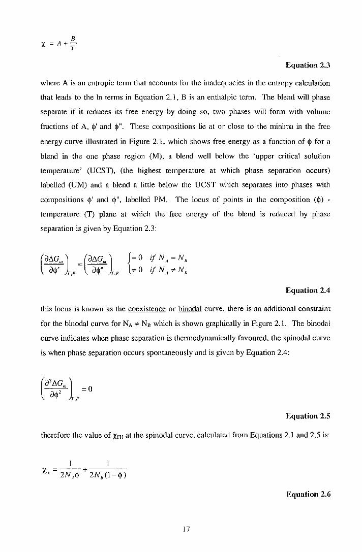
B X = A+
T
Equation 2.3
where A is an entropic tenn that accounts for the inadequacies in the entropy calculation
that leads to the In tenns in Equation 2.1, B is an en thai pic term. The blend will phase
separate if it reduces its free energy by doing so, two phases will fonn with volume
fractions of A, Q>' and Q>". These compositions lie at or close to the minima in the free
energy curve illustrated in Figure 2.1, which shows free energy as a function of Q> for a
blend in the one phase region (M), a blend well below the 'upper critical solution
temperature' (UCST), (the highest temperature at which phase separation occurs)
labelled (UM) and a blend a little below the UCST which separates into phases with
compositions <j>' and Q>", labelled PM. The locus of points in the composition ($) -
temperature (T) plane at which the free energy of the blend is reduced by phase
separation is given by Equation 2.3:
{:~ if NA = NB
if N A~ NB
Equation 2.4
this locus is known as the coexistence or binodal curve, there is an additional constraint
for the binodal curve for NA ~ Nn which is shown graphically in Figure 2.1. The binodal
curve indicates when phase separation is tl1ennodynamically favoured, the spinodal curve
is when phase separation occurs spontaneously and is given by Equation 2.4:
Equation 2.5
therefore the value of :xm at the spinodal curve, calculated from Equations 2.1 and 2.5 is:
1 1 X - +
s 2NA 2N8 (1-$)
Equation 2.6
17

6x1 o-4
Two phase, UM -----.._ Intermediate, PM .,. ....- -...
4 ' One phase, M / ' / ' / ' / ' 2 / ' / ' f- / ' m / ' ..:::L
"- 0 / ' E /
(_') <J
-2 /
/
\ /
/
' /
-4 ' ,./
' -' -
-6 0.0 0.2 0.4 0.6 0.8 1.0
Volume fraction A
Figure 2.:n.: Free ell1ergy of mixirrng for a lbHemD. at varimns JPOnrrnts irn the <!J - 1' phase
diagram. 1'he dD.fferell1t curves are obtairrnedl !by varying Xm· Straight nine is tllle
common tall1gent for <!J' all1dl <!J".
<l.l L
:::J +-' 0 L
<l.l Q_
E <l.l f-
Two Phase ·-...
-·-·-·-·-·-LCST
One Phase
UCST
' ' / '
<P' / ' ' <P'' -~---------------~---
/
/ ' / ' I \
1 Two Phase \ I \
Volume Fraction A
M
PM
UM
\
Figure 2.2: Phase diagram for the situation shown in Figure 2.1, LCST is not
predicted by Flory - Huggins original theory. Solid line - coexistence or binodal
curve, bottom broken line - spinodal curve. l?M, U and M indicated in Figure 2.1.
18

When NA = Nn = N a simple expression is available for XHI at the coexistence curve, xb:
!Equatnon 2.7
The phase diagram of an ideal 'Rory- Huggins' blend is shown in Figure 2.2, this phase
diagram corresponds to the free energy plot in Figure 2.1. Tllis phase diagram exhibits
an upper critical solution temperature (UCST), i.e. the two phase region is found at
lower temperatures. Basic Flory - Huggins theory is only able to predict UCST phase
diagrams, experimentally other behaviours such as lower critical solution temperatures
(LCST), where phase separation occurs at higher temperatures are observed. Note that
the spinodal curve lies inside the coexistence curve.
In the context of the Flory - Huggins theory, de Gennes2 has used the
incompressible random phase approximation to predict the scattering law, S(Q) of a
blend as:
!Equatnon 2.8
where g0 (Rg, Q) is the Debye function3 which describes the intensity of scattering from a
single Gaussian polymer chain with radius of gyration, Rg:
gD (R8 ,Q) = c~2 }exp(-u) + u -1)
u= Q1R1 g
47t Q=-sine
A
Equation 2.9
A is the radiation wavelength and 20 is the scattering angle. The coherent elastic neutron
scatter, I(Q), for a blend, with segment volumes, v A and vn, and scattering lengths bA and
bn, respectively is given b/:
19

Equ.natimn 2.Jl0
Note that the Flory - Huggins interaction parameter, XFH, is replaced by an effective
interaction parameter, x, the reason for this will be discussed shortly. V 0 is a 'reference'
volume:
Equation 2.H
In this situation where the segments have different volumes, the value of Xs is also
modified:
Equation 2.Jl2
If the blend components are not monodisperse but can be described by the Schultz -
Zimm distribution then Equation 2.10 can be used with the substitution of a modified
Debye function5, g'0 (Rg, Q):
Equation 2.13
where u was defined above and:
Mw ( J-1
h= MN -1
Equation 2.14
The complete fom1 of Equation 2.10 can be fitted to scattering data of I(Q), to
obtain X and the radii of gyration of the components. This discussion will continue,
20

concentrating on the scattering structure factor, S(Q). Figure 2.3 shows the effect that
varying the parameters in the mod5.l has on the scattering S(Q), in the fonn of Kratky
plots of Q2S(Q) versus Q. It does appear that the effect of varying the radii of gyration
and the interaction parameter is essentially the same - if this were the case then fitted
values of X would be dete1111ined entirely by the values of the radii of gyration used.
However Figure 2.4 shows that there are in fact differences between the scattering from
a blend with X * 0 and a best fit to the same scattering with X = 0. The discrepancy
between the miginal model data and the best fit with X = 0 is at a maximum for
intermediate values of Q.
0.06
~
a .....___, (f) 0.04 * 0.1
a
0.02
- ·-·-·-· / -- -;. :::. :: -: . - . --:. .
/ ·""' _.... / / -·
I I .· /.
I ,· ... / I i ... · I ,/ I i _.: : // I . : I
I : . /
I i / / I
I i .: . / I ... / I
I . I
I . : I . I : . I
I": . / I : I I
I i ... · : / / ... I I I: : I
/,".·/ / . . ·. /
0.05 0.10 a /A-1
- -·-
0.15 0.20
Figure 2.3a: Scattering for a blends with RgA = Rgn = Rg, tj> = 0.5 and X = 0.
21

-·.:-:-:. :-: .·.-:-:-:.-:--: .·.--;-:-.·.~-·.-:-:- .·.~.-.T"":"
0.06 ... -··-· -· /
----/ ,..--...
/ 0 '-" / (/) 0.04 /
* N / 0 /
X = 0.002 I X = 0.0
0.02 X = -0.002 I X = -0.02
I
0.00 0.00 0.05 0.10 0.15 0.20
Q ;$..-1
Figure 2.31b: ScaUeri111g from blernds with lR.gA = lR.gn = SSA, q> = 0.5 and various X
values.
0.06 ------------,..--... --·---·-·-·-·-·-·-0 '-" (/) 0.04 * N 0
0.02 -- .. -- ..
¢l 0.50 ¢l 0.35 ¢l 0.25 ¢l = 0.10
0 . 0 0 l-<L..L-1-L__L___L__L__j___j__J__J__J__J____J_____J____J___J____J_____J_____J___.J
0.00 0.05 0.10 0.15 0.20 o /A-1
Figure 2.3c: Scattering from blends with RgA = Rgn = 55A, X = 0 and! various ljl
values note for RgA = lRgn blends with composition q> and (.n. - q> ) have the same
scattering function.
22

0.10
0.08
0.06 ,--.... 0 .....__,. (f) 0.04 * N
0
0.02
0.00
Original X = 1 X 1 o-3
Fit to original with X 0 Difference x 1 0
'/ '/
'/ . r·- '
'/
/ /
."V ' ' ."f ' ....
·-·-·-
- 0. 0 2 ,___......__......__......__.L..__.L__.L__....___....___......___.___.__........_........_........_....L..._....L...__L__L___l___J
0.00 0.05 0.10 0.15 0.20 Q ;A.-1
IFUgure 2.4: Scatter from a blend (details in text) with X = .D.x:H.0-3 fitted with an
S(Q) witlh X= 0, along with the difference xlO.
It is possible to approximate Equation 2.8, such that thennodynamic parameters
can be derived from simple linear fits to functions of the scattering data over limited
ranges of the scattering vector Q. For simplicity these approximations will be considered
in the context of a blend with VA = v8 = Vo. At values of Q such that RgQ << 1, the
exponential tenn in the Debye function g0 (Rg, Q) can be replaced by the first tenns of a
series expansion:
Equation 2.15
when this is substituted into Equation 2.8 we obtain:
Equation 2.16
23

where s is the con·elation length for composition fluctuations defined as:
Equation 2.17
a is the statistical segment or Kuhn length of the polymer. To obtain a straight line, s· 1(Q) is plotted versus Q2
, the intercept of this line is 2(Xs- X) and the gradient is 2s2(Xs
X) (or s2 = (gradient/intercept)). This is sometimes known as the Ornstein - Zernike
plot. At high Q, g0 (Rg, Q) becomes small and the -2X term negligible and therefore:
Equation 2.18
hence the statistical segment length can be obtained from the gradient of the high Q
region of the Ornstein - Zemike plot. However if the scatter from a single coil deviates
from the Debye function erroneous values for the statistical segment length will be
obtained.
There are three main assumptions made in these derivations for the scattering
behaviour of a polymer blend:
(i) The blend can be described by the Flory - Huggins lattice.
(ii) The incompressible random phase approximation applies - this assumes that there is
no change in the total volume of the system when the pure components are mixed.
(iii) The chains have a Gaussian distJ.ibution of segments and so the scattering from a
single chain can be described by the Debye function.
In practice all of these approximations are violated to some extent. The Flory _
Huggins theory is known to fail, in that is not able to predict any phase behaviour other
than UCST behaviour. This occurs for a number of reasons; the physical 'un
naturalness' of the lattice, the discounting of specific interactions, the assumptions made
in calculating the entropy of mixing and so fmth. A number of attempts have been made
to modify the Flory - Huggins theory, by taking into account the presence of free
volume6, differing surface areas for the different segment types7
, the presence of
composition fluctuations8, and adding structure to the individual segments by spreading
each segment across several lattice cells (lattice cluster theory)9• Additionally there have
24

also been Monte Carlo simulations 10 '11
, polymer reference interaction site models
(PRISM) 12, Born - Green - Yvon integral equation treatments 13 and equation of state
theories14. These various theories are reviewed and compared by Binder15 and Cui and
Donohue16, it is beyond the scope of this work to desc1ibe these various theories and the
intention is simply to provide a starting point for any further study and give some idea as
to the amount of theoretical activity there is in this important area. The overall
conclusion that can be drawn from these various articles is that the interaction parameter
that is extracted from Small Angle Neutron Scattering (SANS) data is not the simple XH-1
described in Equation 2.2, but is a function of both composition and molecular weight.
However these more recent theories offer no new, straightforward method to analyse
SANS data. For this work the most useful ideas have been those of Kumar10 who has
considered the effect of volume changes on mixing, and found that for 'repulsive' blends
where there is a slightly unfavourable interaction, such as in the blends of a polymer with
it's deuterated isomer, a small increase in volume is expected leading to slight increases
in the effective X parameter at the limits of the composition range. For 'attractive'
blends, on the other hand, a small decrease in volume on mixing is expected and this
leads to a downturn in the effective X parameter at the limits of the composition range.
Examples of 'attractive' blends would include poly (ethylene oxide) I poly (methyl
methacrylate) and polystyrene I poly (vinyl metl1yl ether). These ideas are also
incorporated in tl1e compressible Random Phase Approximation of Tang and Freed17.
Turning finally to the third assumption, that the segment distribution is Gaussian,
this assumption is obeyed moderately well for polystyrene but for other polymers, such
as poly (methyl methacrylate) it does breakdown, generally this occurs at intermediate
and higher values of Q. A better prediction of the segment distribution and thus the
single coil scattering of a polymer chain is obtained using the Rotational Isomeric State
(RIS) model of Flor/ 8 , again the problem is that this gives no simple analytic form for
the single coil scattering function.
25

2.2 Surface Enrichment
Figure 2.5 shows a schematic phase diagram of a simple binary polymer blend, with
components A and B. If we consider such a blend with a bulk composition
corresponding to one of the coexisting phases, X for example, then under certain
circumstances the other coexisting phase Y will be found to be preferentially absorbed at
the 'walls' of the container in which the blend resides. The component with the lower
surface energy will be expected to be found at the smface. Two sorts of wetting
behaviour are expected: firstly the wetting layer may be thick, this will occur close to
the critical point of unmixing and secondly as the blend is moved away from the critical
point of umnixing along the coexistence curve a transition, W, to a much thinner
'partially' wet state will occur. The transition between these two states may be, in
theory, first or second order. A precursor phenomena, often called 'prewetting', will
sometimes be observed in the one phase region close to the coexistence curve. The type
of transition that is observed and its location on the coexistence curve will be detennined
by the thennodynmnics of the blend; the interactions between the component polymers
and the relative strengths of their interactions with the container wall.
One Phase Region
Temperature
Wet
]itical unmixing
0 X Volume Fraction A Y
Figure 2.5: Phase diagram for a simple binary blend
26
1

The surface enrichment behaviour of a blend can be analysed by writing an
expression for the free energy of the blend, incorporating contributions from the bulk, a
smface energy contribution and a contribution accounting for the free energy cost of
maintaining composition gradients in the blend. The general themy for blends was
discussed by Cahn19, a theory for polymers based on the Amy - Huggins lattice
representation of the blend was presented by Nakanishi and Pincus20 and Schmidt and
Binder21• Subsequently Cannesin and Noolandi22 have used an integral representation
of the polymer blend in the same context. Jones and Kramer23 have made
approximations to the theory of Schmidt and Binder that allow some results to be
obtained from simple analytical expressions. The main concem here is the shape of the
near smface composition profile, the derivations presented here are drawn broadly from
all the above references. The form of the transition between partial wet and wet state is
not discussed here, the nature and location of this n·ansition is discussed further by
Jones24•
The expression for the free energy of a two component polymer blend, on a simple
cubic Aory - Huggins lattice, including a surface energy contribution is:
11G J l <j> (1- <j> ) a 2 l k
8 T = fs ( <J> air)+
0 d1 N A ln <J> + N
8 ln(l- <J> ) + X FH <j> (1- <j> ) - 1111<1> + 36<1> (1- <j> ) (V <j> )
2 J
NA ,Nn are the degrees ofpolymerisation of A and B respectively.
a is the statistical segment length.
<1> is the volume fraction of component A
XFH is the Flory- Huggins interaction parameter.
Equation 2.19
1111 is the exchange chemical potential evaluated at the bulk composition.
fs(<J>air) is the surface free energy conuibution, the surface composition is <!>air·
This expression assumes a semi - infinite system with an interface located at z = 0, the
final term in the expression is the contribution to the free energy from concentration
gradients. This term is valid only in the long wavelength approximation:
Equation 2.20
27

where N = NA = N13 • i.e. the concentration gradients in the bulk are not sharp. It is also
assumed that the system is isotropic in the x-y plane, hence:
Equation 2.21
In general it is assumed that the surface free energy contribution is localised at the
surface as a 8 - function and so only depends on the smface composition. This
approximation makes the ensuing maths more manageable and is not umeasonable.
Chen, Noolandi and Izzo25 discuss the effect of a non-8-function surface free energy.
fs(<l>air), can be expressed as the first two terms of a Taylor series in <l>air:
Equation 2.22
!11 is related to the smface energy difference, D..y, between components A and B:
Equation 2.23
Where b is the parameter of the Flory - Huggins lattice. g is known as the 'missing
bond' tenn and is equal to -XFHb. To find the composition profile within the blend we
must minimise the free energy given by Equation 2.19 with respect to <j>. Variational
calculus shows that this free energy minimum is obtained when:
Equation 2.24
This is known as the 'phase portrait'. The boundary conditions at z = 0 and z -7 oo are
used to find <l>air and indicate which solutions of Equation 2.19 aTe acceptable and also
28

gives an indication as to what physical situation they represent. Using these boundruy
conditions Equation 2.24 becomes:
+ th . = + a rli1G"' (<!>air ' X FH) - 11G"' ( <!> lJ ' X FH) - 1111 (<!>air - <!> lJ) ]1/l ll-1 g't'mr -3 th. (1-tl-. . )
'f mr 'f a1r
Equation 2.25
<!>B is the bulk volume fraction of component A (i.e. when z--joo). I1G111 (<J>,XFH) is the
Gibbs free energy per lattice site:
Equatnonll 2.26
By plotting both sides of Equation 2.25 together, as a function of <!>air, the crossing
points give possible values of values <!>air and the areas bisected indicate the physical
situation which will be observed. Figures 2.6 are exrunples of this type of plot, both
figures represent a situation with a blend at the coexistence curve (i.e. 1111 = 0 for a blend
with NA = NB). <J>,;;rl ,<J>,!·r and <J>.~r are possible values for the surface volume fraction, in
fact <J> .:r is at a maximum in the free energy and so is unstable. <j> a~r is the smface volume
fraction in the partial wet case, i.e. the volume fraction decays directly from the surface,
and <j> .~r is the surface volume fraction in the wet case, i.e. with a thick uniform layer at
the surface. The solution which occurs, wet or partially wet, depends on the relative
areas W and PW. If area PW is larger than area W then , the partial wet state, <j> a~r is the
correct solution and if area W is larger than area PW then , the wet state, t~-. c. is the 'i'mr
correct solution. So in this case Figure 2.6a represents a blend where complete wetting
is occurring and Figure 2.6b partial wetting, in this illustration the transition is driven by
a change in the surface energy difference. These diagrams can also be used to work out
the location and type of transition between the wet and partial wet states.
29

0.08
>-.. ~ 0.06 <1)
c <1)
<1) <1) 0.04 L
LL
0.02
0.2 0.4 0.6 0.8 1.0 Surface Volume fraction, ¢air
Figure 2.6a: l?tnase portraut lfor a blend on the coexustence curve exhubiting
compnete wetting, with s11.11rface vo!ume fraction, <j> .~,.
0.08
>-.. ~ 0 06 <1) •
c <1)
<1) <1) 0.04 L
LL
0.02
0.2 0.4 0.6 0.8 1.0 Surface Volume fraction, ¢air
Figure 2.6b: Phase portrait for the same blend as above, in this instance exhibiting
partial wetting, due to a reduction in the surface energy difference, surface volume
fraction, ,~, " . 'f 111r
30
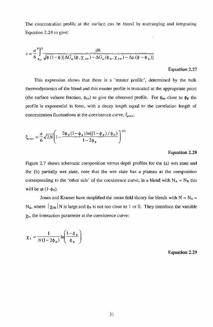
The concentration profile at the smface can be found by rearranging and integrating
Equation 2.24 to give:
Equation 2.27
This expression shows that there is a 'master profile', determined by the bulk
thermodynamics of the blend and this master profile is truncated at the appropriate point
(the surface volume fraction, <Pair) to give the observed profile. For <Pair close to <Ps the
profile is exponential in fonn, with a decay length equal to the correlation length of
concentration fluctuations at the coexistence curve, ~oex:
Equation 2.28
Figure 2.7 shows schematic composition versus depth profiles for the (a) wet state and
the (b) partially wet state, note that the wet state has a plateau at the composition
corresponding to the 'other side' of the coexistence curve, in a blend with NA == Ns this
will be at (1-<J>s).
Jones and Kramer have simplified the mean field theory for blends with N == NA =
Ns, where I XFH IN is large and <Psis not too close to 1 or 0. They introduce the variable
xb, the interaction parameter at the coexistence curve:
Equation 2.29
31

. c 0
:..::; 0 0 L
'+-
<ll
E ::J 0 >
Depth
Figure 2./a: A 'wet' profile, note tlhat the plateau region is at vonume fraction (1 -
cl>n) for a symmetric !blend and! is of indeterminate thickness irn the Sclhmidlt and
Binder formulation.
-c 0
:..::; 0 0 L
'+-
<ll
E ::J
0 >
Depth
Figure 2.7b: A 'partial wet' profile, note that the surface volume fraction is less
than (1 - cpn) for a symmetric blemD, the nength scale of tlh.e decay is of the order of
the radius of gyration of the enriching polymer.
32

The smface volume fraction for the wetting profile is given by:
<l>n + t <Pair = 1 + f
where the parameter, t, is given by:
and the composition profile is obtained from the expression:
EquaHmn 2.30
Equation 2.3]_
Equation 2.32
In addition to these models based on the theory of Calm, there are also self consistent
field theories26 '27 and Monte Carlo simulations28
•29
'30
. (It is possible to use the
LAYERS program, used in section 2.3.1 to do self consistent field calculations for
surface enrichment.)
There is good agreement between Monte Carlo models and the mean field theory,
the small deviations observed can be attributed to the effect of fmite compressibility and
distortion of polymer chains at the surface from the ideal Gaussian chain segment
distribution, the mean field takes no account of these effects.
The self consistent field theory of Hariharan et aP6 has been used to study the
effects of chain length disparity (NA "# NB), a small entropic effect is observed, whereby
the shorter chains are found preferentially at the surface in the absence of a surface
energy difference. For long chains this amounts to a smface composition different from
the bulk by only 1% or so.
33

2.3 Polymer Brushes
A polymer bmsh is fanned when polymer chains 'end absorb' to an interface, this
'bmsh' may significantly alter the properties of the intetface. Commonly such bmshes
have been considered in the context of polymers in solution end absorbing onto some
substrate, in this work the interest is in two component polymer blends where one
component has a low surface energy end group and that is intended to fonn brushes at
the blend I air interface. These two different situations are known as 'wet' brushes,
where the polymer is in solution (or the molecular weight of the manix polymer is less
than that of the brush polymer), and 'dry' bmshes, where the 'solvent' is another
polymer (with molecular weight higher than that of the brush fanning polymer). Two
theoretical methods of n·eating brushes are considered; a self consistent field (SCF)
theory developed by Shull31 '32
, based on the mean field ideas originating from
Edwards33 and the self consistent field methods of Scheutjens and Fleer34 and a scaling
theory developed by de Gennes35.
2.3.1 Self Consistent Field Theory
All the models presented here were obtained usmg the program LAYERS,
written by K.R. Shull.
We will consider a two component polymer blend with components A, a
homopolymer with degree of polymerisation NA and component B a polymer with degree
of polymerisation N8 and a smface active group at one encl. The discussion here
concentrates on a component B with only one smface active end group, for clarity,
however the modifications for a surface active end group at each end are relatively
straight forward and have been included in the program LAYERS. The blend is
characterised by a Flory - Huggins interaction parameter, XFH·
This binary blend exists on a Flory - Huggins like cubic lattice with an
impenetrable interface at x = 0, x is the number of lattice layers from this impenetrable
surface. For the purposes of the calculations in this work the number of layers, Xn, in the
lattice is not important so long as the brush has reached bulk composition well before
(i.e. 5-10 layers) the far edge of the lattice is reached.
34

The interaction of the smface active end is characterised by two parameters, xb~
is the interaction of the ends with the bulk of the blend and Xse is the interaction of the
ends with the surface, so the ends may be found at the smface because they have been
'expelled' by the bulk or because they feel an attraction to the surface. It is the
difference Xbe_Xse that detennines the number of Bends absorbed at the surface.
The quantities of interest are the volume fractions of components A and B as a
function of x, ~A(x) and ~s(x). These values are calculated from the distribution
functions qA(x,j), qsi(x,j) and qs2Cx,j). qk(x,j) is the probability that a chain has reached
position x, after j steps along its length from end k. Two functions are required to
describe the B component because the two ends of the B chains are distinct- one end has
a surface active group (q81 (x,j)) and the other does not (qn2(x,j)). The volume fractions
are calculated from the qk(x,j) thus:
~A (x) = AAtA q A (x,j)qA (x,N A- j)dj 0
Equation 2.33
Equation 2.34
Ak are nonnalisation constants. The distribution functions qk(x,j) are analogous
to concenn·ation, in a modified diffusion equation:
Equation 2.35
Wt(x) is a mean field acting on the polymer segments, ansmg from the
neighbouring segments. In fact Equation 2.35 is based on a continuous fmm for qk(x,j)
35

and not the discrete fonn implied by the lattice on which the polymers are placed. The
discrete fonn for Equation 2.35 is given by the following recursion relations:
EquatUon 2.36
The tenns in qk(x,j) occur by virtue of the chain connectivity, each chain segment
has six nearest neighbours one each in the layers x-1 and x+1 and four in the layer x and
the probability qk(x,j) depends on the probabilities of the previous segment, j-1, being in
any of the neighbouring cells. The exponential is a Boltzmann distribution function,
evaluating the probability of finding a polymer segment in a state with energy wk(x),
from the mean field. The only unknowns in this set of equations are the mean fields,
since all the values qk(x,j) can be calculated using the following initial conditions:
qA (x,O) = 1}
q 81 (x,O) : 1 x = 1 ~ x"
q82 (x,O) -1
qA (O,j) = 0,
qBl (O,j) = 0,
q82(0,j) = 0,
q A (n + 1, j) = 0 }
q81 (n+1,j~=0 j=0~max(NA,N8 )
q 82 (n + 1, J) = 0
Equation 2.37
Equation 2.38
Equation 2.37 is a 'book-keeping' boundary condition, so that the chain
connectivity of the end groups is accounted for properly. Equation 2.38 expresses the
36

fact that no chain segments lie beyond the polymer layer, they are a confinement
condition. In addition the following conditions apply for first segments in the bulk of the
lattice i.e. not in layer 1:
Equation 2.39
Finally there are the conditions for first segments in the surface layer:
(-wA (x)J 1 q A (x,1) = exp kBT
(
s wB(x)Jl qBi (x,1) = exp -Xe - kBT rx = 1
(-w8 (x) J Jl
q B2 (x,1) = exp kBT
The mean fields WA(x) and ws(x) can be divided in two parts:
wA (x) = w~ (x)- w'(x)
w8 (x) = w~ (x)- w'(x)
Equation 2.40
Equation 2.41
The difference between these mean fields lies solely in the Wk0 (x) parts which are
given by:
w~ (x) = XFH<P~ (x)
lV~ (x) = XFu<P~ (x)- wext (x)
Equation 2.42
37

The tem1 Wex1(x) is a field that acts equally on all B segments not arising from A
B interactions, for 'pure' brushes this tenn is zero but it can be used to include a
preferential attraction to the interface of A or B segments. This allows us to study both
surface enrichment where composition gradients are driven by differences between the
surface energies of the chain segments and brushes where composition gradients are
driven by end absorption, in addition it is also possible to consider combinations of these
effects.
w'(x) is given by:
<!>bulk <!>bulk w'(x)=~(l-<!>A(x)-$8 (X))+ ~ + ~
A B
Equation 2.43
s is inversely proportional to the bulk compressibility and <!>Abulk and <l>sbulk are the bulk
volume fractions of components A and B respectively. The procedure to calculate the
equilibrium volume fraction profile is firstly to calculate volume fractions <!>A(x) and <!>s(x)
using an initial estimate for the mean fields based on the assumed bulk volume fractions,
wk(x). These calculated volume fractions are used to detennine a new set of 'image'
mean fields, wkl(x). New values for the mean fields are calculated from a linear
combination of wk(x) and wkl(x), this procedure is repeated until some convergence
critelia is met.
The preceding section outlined the details of the mechanics of the self consistent
field theory calculations. Some results will now be discussed, there are a number of
factors influencing the size and shape of the near surface composition profile these are:
(a) The value of (Xeb- Xe5), this is the enthalpic contribution to the end attachment free
energy, larger values will result in larger values of the surface excess.
(b) Nn and the ratio NAINn, smaller values of Ns will enlumce brush fonnation since the
entropic cost of confining the end of a shorter chain to the interface is smaller than that
for longer chains. Larger ratios of NAf'Ns will also enhance brush formation.
(c) XFH, the Flory- Huggins interaction parameter, all the modelling work done here was
in the one phase region of the phase diagram. Brush fonnation is enhanced in blends that
lie closer to the coexistence curve, i.e. with small positive values of XfH.
(d) The bulk volume fraction, <l>s (= <l>s bulk), of the brush forming polymer.
38

Figure 2.8 illustrates some typical composition versus depth profiles. The data
here are shown versus lattice layer, but the depth z is often nonnalised by the radius of
gyration, Rg, of the brush forming polymer, as part of the procedure used to relate results
obtained theoretically, which for computational tractability are done on polymers with
relatively small values of NA and NB, to the experimental data.
1.0 '-
' p 6.5 ' p 4.5
'\ 0.8 \ ~
2.5 1.5
OJ ' \ p 0.5 ' \ c ' \ 0 ' \ -+-'
() '\ \ \
0 \ \ L. '\ \ 'I- \
' Q) ' \ 0.4 ' E ' ' ' ' ' ::J ' ' ' - " '- ' 0 -- .. - " ·- ~ ~-.-~~~~--=--> 0.2
Lattice layer
Figure 2.8 Example brush profiles for a series of model blends with NA = N8 = 100,
cjl8 = 0.25 and x = 0, the free energy of end attachment, ~' is defined in Equation
2.44.
Throughout this work two parameters will be used to characterise the shape of the
composition profiles - these are the nonnalised surface excess z*/Rg and the difference
between the surface, ~air. and bulk, ~B. composition (~air - ~B). Figure 2.9 shows a plot
of (~air - ~B) vs z*/Rg for two series of calculations, firstly where ~B is fixed and the
enthalpic attachment energy increased (leading to an increasing z*/Rg) and secondly
where the enthalpic attachment energy is fixed and ~B is increased (similarly leading to an
increasing z*/Rg), for small values of z*/Rg the two curves overlay but at higher values the
data with varying ~B 'curl over'. This is because the excess is constrained to be zero
when ~B is one, so there must be a maximum in z*/Rg with respect to ~B. this is illustrated
in Figure 2.1 0.
39

0.4
CD 0.3 -& I .!::: 0
-& 0.2
0.1
-Varying {J 0 Varying ¢>8
0 a
0. 0 "--...J....___L_____L_.L.._....J.___J_---'-.J...._-'-____L-L..._...J....___L_____L_.L.._....J
0.0 0.2 0.4 0.6 0.8
Normalised Excess z'•/R9
Fngu.ure 2.9: ($air - $8 ) versus normalised excess for two series of lbRends: (]_) the
excess is increased by increasing the attachment fr·ee energy and (2) the excess is
increased by increasing the bulk volume fraction of the absorbing polymer.
1.5 I I I I I I
Ol 0 {J= 2.95, x= o.o 0:::: t::. P= 1.45, x= o.oo6 ....._.,__ + P= 1.45, x= o.o .. x P= -o.o5, x= o.o N
u) 1.0 t- -en 0 0
Q) 0
u X 0 0 Q)
A A 0
""0 Q) 0 A A en 0.5 - -+ + A 0 + +
E A + L + 0 z A
+ )(
)( )( )(
)(
0.0 )( i I I I I I
0.0 0.1 0.2 0.3 0.4 0.5 0.6 0.7 Bulk volume fraction, cl>s
Figure 2.10: Normalised excess, z*/Rg, versus cj>8 showing the maximum in z*/Rg
which arises at intermediate $B· Brush formation occurs at f3 < 0, stabilised by
entropy of mixing in the plane of the surface.
40
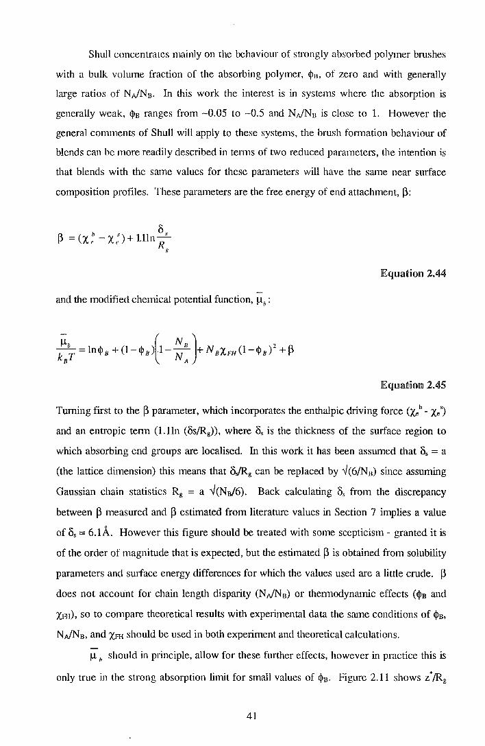
Shull concentrates mainly on the behaviour of strongly absorbed polymer brushes
with a bulk volume fraction of the absorbing polymer, ~B. of zero and with generally
large ratios of NAfN 13 • In this work the interest is in systems where the absorption is
generally weak, ~B ranges from ~0.05 to ~0.5 and NAINB is close to 1. However the
general comments of Shull will apply to these systems, the brush fonnation behaviour of
blends can be more readily described in tenns of two reduced parameters, the jntention is
that blends with the same values for these parameters will have the same near surface
composition profiles. These parameters are the free energy of end attachment, ~:
Equation 2.44
and the modified chemical potential function, ~b:
EqlllatnoHll 2.45
Turning first to the~ parameter, which incorporates the enthalpic driving force (Xeb- XeJ
and an entropic term (l.lln (8s/Rg)), where 8. is the thickness of the surface region to
which absorbing end groups are localised. In this work it has been assumed that 8. = a
(the lattice dimension) this means that 8s!Rg can be replaced by -,J(6/N13) since assuming
Gaussian chain statistics Rg = a -,J(Ns/6). Back calculating 8s from the discrepancy
between ~ measured and ~ estimated from literature values in Section 7 implies a value
of 8. = 6.1A. However this figure should be treated with some scepticism- granted it is
of the order of magnitude that is expected, but the estimated ~ is obtained from solubility
parameters and surface energy differences for which the values used are a little crude. ~
does not account for chain length disparity (NAIN 13) or thennodynamic effects (~13 and
Xffi), so to compare theoretical results with experimental data the same conditions of <j>13 ,
NAfN13 , and XFH should be used in both experiment and theoretical calculations.
11 h should in principle, allow for these further effects, however in practice this is
only true in the strong absorption limit for small values of ~13 • Figure 2.11 shows z*/Rg
41
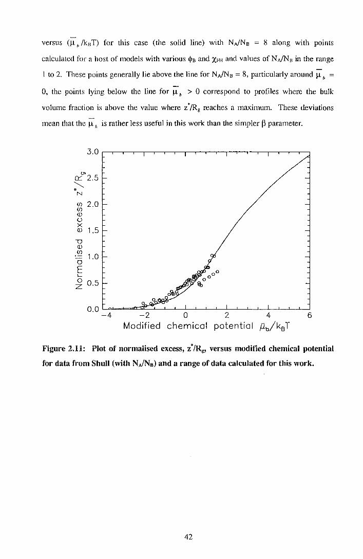
versus (!l h /knT) for this case (the solid line) with N.JNn = 8 along with points
calculated for a host of models with various IJ>B and XH-1 and values of N.JNB in the range
1 to 2. These points generally lie above the line for N.JNB = 8, pruticularly around ll b =
0, the points lying below the line for ll b > 0 correspond to profiles where the bulk
volume fraction is above the value where z*/Rg reaches a maximum. These deviations
mean that the ll h is rather less useful in this work than the simpler p parruneter.
Ol 0:::: 2. 5 ~ * N
(f) 2.0 (f) ())
0 X ()) 1.5
"""0 ()) (f)
0
E L
1.0
~ 0.5
0. 0 L.o.J~=z:st~::::::......___L____..L___i___L_...J..___L__.l_J__l___jc___j____L__L___L._j
-4 -2 0 2 4 6
Modified chemical potential P,b/k8 T
Figure 2.11: Plot of normalised excess, z"/Rg, versus modified chemical potential
for data from Shull (with NA/NB) and a range of data calculated for this work.
42

2.3.2 Scaling 'fheory
The basics of the scaling theory of polymer brushes will be introduced, however
this must be done with the understanding that the results will only give, at best, a feel for
the underlying behaviour of the brushes observed in this work. The reason for this is that
scaling theory is not able to account properly for the entropy of mixing between the
brush fanning polymer NB with the manix polymer NA, when NA > NB. Additionally it is
assumed in scaling theory that the brush composition depth profile is a step function, self
consistent field theories36 and Monte Carlo studies37 '38 show that this is not the case.
This outline of scaling theory draws on the paper by de Gennes35, who considers
the end absorption of polymers with NB repeat units to a solid surface, in a solution of
'mobile' polymers with NA repeat units. So the system consists of absorbed polymers,
mobile polymers and a solvent, in de Gennes paper the mobile polymers are referred to
as P, rather than NA. The notation used here is to remain consistent with the preceding
section on self consistent field theory. The important parameters in the scaling theory
are the dimensionless grafting density, cr, and the volume fraction of mobile chains, ~·
The size of the lattice cell is a and the height of the grafted brush is L. A further
parameter, 0 0 , the distance between graft points is also defined:
Equation 2.46
The results of de Gennes are summarised in Figure 2.12. This figure shows where
sn·etching of the grafted chains from their unperturbed dimensions occurs (US -
unstretched, WS - weakly stretched and SS - strongly sn·etched) and where mixing
between the grafted chains and the mobile chains is predicted (M - mixed and UM -
unmixed). The extreme left of this diagram(~= 0) conesponds to a grafted polymer in a
pure solvent with no mobile chains.
43

1
SS.UM
a
Ns-6/5
US.UM US.M
0 0 --<j>---1> 1
Pure solvent Melt
Figure 2J.2: Schematic representation of de Gennes scaling results for brushes
(from reference 35).
There are two regimes predicted in this case, the unsu·etched regime where chains are
grafted sufficiently far apart that they do not overlap, it can be shown that this is when a
< NB-615
. In this situation the brush height, L ""' Ns315 a, the dimensions of a chain in a
good solvent. When the grafted chains overlap they are stretched out away from the
surface and the brush height is found to scale as:
L- N aa 113 - B
Equation 2.47
Both of these chains are denoted UM because there are no mobile chains to mix with!
The polymer melt case appears on the far right of Figure 2.12, where <1> = 1. The
behaviour in this case is slightly more complex, again at the lowest grafting densities
chains do not peneu·ate and so as long as NA > N81r- they have ideal dimensions and the
length of the brush will be given by L ""' N 8 112a. Clearly the mobile chains can easily
penetrate this brush. The cross over to the stretched regime is different to that for the
44

polymer - pure solvent system, as the grafting density increases the absorbed chains will
start to overlap, however- initially they will not be stretched because the penetration of
the mobile chains screens interactions between the grafted chains. It can be shown that
stretching of the grafted chains starts to occur when:
- N N-312 (J- A B
Equatfimn 2.48
At this point the grafted layer is still mixed with the mobile chains. The final regime is
reached when' mobile chains are expelled from the grafted layer, ultimately as the graft
density reaches one the brush length will be L "" aNB. The cross over to the regime
where this occurs is when:
r<-N-lt2 v- A
Equation 2.49
For NA = NB the stretched mixed regime (WS.M) will not exist since NANB-312 = NA-112•
The free energy of the grafted brush in the melt can be calculated by summing the free
energy of mixing ~Gm and the elastic energy ~Ge1 of the brush, (the equations used here
are those of Brown39, which include a non-zero interaction parameter, XfH). The free
energy of mixing tenn is given by:
Equation 2.50
and the elastic energy is given by:
Eqmation 2.51
45
Minimising ~Gm + ~Ge1 with respect to the volume fraction of NB in the brush, <J>B, gives
Equation 2.52 below. (In the context of the scaling theory the composition of the brush
is unifonn)
EquatioHll 2.52
This relates the volume fraction of the grafted polymer in the brush, <J>B, to the
parameters cr, NB, NA and XHI· The brush height is given by:
Equation 2.53
These expressions fail for NA > NB, because the expression for ~Gm is no longer
accurate. The remainder of Figure 2.12 represents the semidilute regime where there is
absorbed polymer, mobile polymer and solvent present, de Gennes discusses the
behaviour in this region in some detail.
46
2.4 /References io Seciion 2
1. P.J. Flory, 'Principles of Polymer Chemistry', Cornell University Press, 1953.
2. P.G. de Gennes, 'Scaling Concepts in Polymer Physics', Cornell University Press,
1979.
3. P. Debye, Journal of Physical Colloid Chemistly, 51, .lL94l7, 18.
4. M. Shibayama, H. Yang, R.S. Stein, C.C. Han, Macromolecules, 18, 1985,2179.
5. S. Sakurai, H. Hasegawa, T. Hashimoto, I. Glen Hargis, S.L. Aggarwai, C.C. Han,
Macromolecules, 23, 1990, 451.
6. M.G. Bawendi, K.F. Freed, Journal of Chemical Physics, 88(4), 1988,2741.
7. G. Beaucage, R.S. Stein, R. Koningsveld, Macromolecules, 26, 1993, 1603.
8. M. Muthukumar, Journal of Chemical Physics, 85(8), 1986, 4722.
9. J. Dudowicz, K.F. Freed, Macromolecules, 24, 1991, 5074.
10. S.K. Kumar, Macromolecules, 27, 1994, 260.
11. A. Sariban, K. Binder, Macromolecules, 21, 1988,711.
12. A. Yethiraj, K.S. Schweizer, Journal of Chemical Physics, 98(11), 1993,9080.
13 . H.M. Sevian, P.K. Brazhnik, J.E.G. Lipson, Journal of Chemical Physics, 99(5),
1993, 4112.
14. I.C. Sanchez, R.H. Lacombe, Macromolecules, 11, 1978, 1145.
15. K. Binder, Advances in Polymer Science, 112, 1994, 181.
16. Y. Cui, M.D. Donohue, Macromolecules, 25, 1992, 6489.
17 . H. Tang, K.F. Freed, Macromolecules, 24, 1991, 958.
18. D.Y. Yoon, P.J. Flory, Macromolecules, 9, 1976,299.
19. J.W. Cahn, Journal of Chemical Physics, 66(8), 1977, 3667.
20. H. Nakanishi, P. Pincus, Journal of Chemical Physics, 79(2), 1983, 997.
21 . I. Schmidt, K. Binder, Journal de Physique, 46, 1985, 1631.
22. I. Carmesin, J. Noolandi, Macromolecules, 22, 1989, 1689.
23 . R.A.L. Jones, E.J. Kramer, Polymer, 34(1), 1993, 115.
24. R.A.L. Jones, Polymer, 35(10), 1994, 2160.
25 . Z. Y. Chen, J. Noolandi, D. Izzo, Physical Review Letters, 66(6), 1991, 727.
26. A. Hariharan, S.K. Kumar, T.P. Russell, Macromolecules, 24, 1991, 4909.
27 . A. Hariharan, S.K. Kumar, T.P. Russell, Macromolecules, 23, 1990, 3584.
28. P. Cifra, F.E. Karasz, W.J. MacKnight, Macromolecules, 25, 1992, 3895.
47

29. J.-S. Wang, K. Binder, Journal of Chemical Physics, 94(12), 1991, 8537.
30. P. Cifra, F. Bruder, R. Brenn, Journal of Chemical Physics, 99(5), 1993,4121.
31. K.R. Shull, Journal of Chemical Physics, 94(8), R99R, 5723.
32. K.R. Shull, E.J. Kramer, Macromolecules, 23, 1990, 4769.
33. S.F. Edwards, Proceedings of the Physical Society, 85, 1965, 613.
34. J.M.H.M. Scheutjens, G.J. Fleer, Journal of Physical Chemistry, 84, 1980, 178.
35. P.G. de Gennes, Macromolecules, 13, R980, 1069.
36. S.T. Milner, T.A. Witten, M.E. Cates, Macromolecules, 21, 1988, 2610.
37. P-Y. Lai, K. Binder, Journal of Chemical Physics, 97, 1992,586.
38 . T. Cosgrove, T .. Heath, B. van Lent, F. Leermakers, J. Scheutjens,
Macromolecules, 20, 1987, 1692.
39. H.R. Brown, K. Char, V.R. Deline, Macromolecules, 23, R990, 3385.
48

This page left intentionally blank
49

3. 7l /Neutroru Techruiques
All the neutron scattering (small angle and reflectivity) done in this work was
carried out at the Ruthetford Appleton Laboratory, Chilton. At this source neutrons are
produced by 'spallation'. Protons are accelerated to high energies ( -800Me V) in a
synchrotron and then fired at a tantalum or uranium target, neutrons are 'chipped off' or
'spalled' from the target nuclei, the yield is around 25-30 per incident proton. Initially
the neutrons have a high energy ( -40Me V), but they are passed through a moderator
where they are thennalised by repeated collisions to give a Maxwell - Boltzmann
distribution of energies. For this work a liquid hydrogen moderator is used which is at a
temperature of 22K. The most probable neutron energy, Emax, in the Maxwell -
Boltzmann distribution is given by:
Equation 3.1
Where k8 is the Boltzmann constant and T is the absolute temperature. The velocity of
neutrons with such energy is given by:
V = (2£max .Jl/2 max nl
II
Equation 3.2
where 111n is the neutron mass ( = 1. 7 x 10-27 kg). For the 22K hydrogen moderator this
corresponds to a velocity of -7 40 m s-1, the wavelength of a particle I wave such as the
neutron, with velocity, v, is given by the de Broglie relationship:
'A=_!:_ m,.v
Equation 3.3
so

where his Planck's constant. For the most probable energy in the distribution from the
hydrogen moderator this wavelength is -5.4A. The finite velocity of the neutron, which
determines its wavelength, leads to the manner in which neutrons of different wavelength
are discriminated at the Rutherford Appleton Laboratory. The proton beam does not
bombard the target continuously, instead very short pulses are used at a rate of 50Hz.
This means that bunches of neutrons leave the target at known times, they then travel
through the experiment and are detected. Shorter wavelength neutrons travel faster than
longer wavelength neutrons and so the first neutrons to arrive at the detector from any
pulse of neutrons are those of shortest wavelength, i.e. wavelengths are detennined by
time of flight.
A particular wavelength range can be selected by the use of a 'chopper', a
chopper is a disc of material (fairly) opaque to neutrons (see Figure 3.1) that has a
segment cut out of it. This disk rotates at 50Hz and is synchronised with the arrival of
the proton pulse at the target such that when neutrons of the conect velocity arrive the
segment cut out of the disk is in the path of neutron beam, other neutrons with the
wrong velocity, miss the gap and are stopped.
Neutrons
Chopper
······~
Axis of rotation
Figure 3.1: Schematic diagram of a disk chopper, allowing the passage of desirable
neutrons.
A general review of the various experiments that can be performed on polymers
using neutrons is by Higgins and Benoie .
51

3.lt.ll §maiD Angle Neutron Scattering (SANS)
The aim of a small angle neutron scattering experiment 1s to measure the
'normalised' flux of neutrons scattered through scattering vectors Q (= (4n/A)sin 8).
Normalised by both the incident neutron flux and the volume of the sample. The
particular interest in this work is neutrons that have been scattered elastically (i.e. with
no energy loss) and coherently (that is neutrons arising from the interference between
neutrons scattered from two different points in the sample). This elastic coherent scatter
contains information on the 'structural' correlations in the sample. To take a polymer
blend, with components A and B, as an example and imagine standing on a segment of
type A, the segments closest to this 'home' segment will most probably also be of type
A, in the same chain as the 'home' segment. The exact disuibution of other A segments
as a function of distance from the 'home' segment will depend on the conformation of
the polymer chain and so the small angle scattering is sensitive to the chain confonnation.
If, in addition, there are interactions between chains of type A then there will be
an additional structural correlation for distances beyond the polymer chain in which the
'home' segment lies, this inter- molecular correlation will also influence the scattering.
The following paragraphs are an attempt to introduce the principal mathematical
relationships that define the scattering, the details of the scattering arising from polymer
blends are given in Section 2.1. This section is by necessity highly summarised,
Lovesel gives a more in depth presentation of the fundamentals of neutron scattering.
In this section vector quantities will appear in bold type and scalar quantities in nonnal
type.
Neutrons behave as if they are scattered from a so called Fenni pseudo potential,
V(r), which is given by:
h2 V(r) = --b8 (r- R)
2nm"
Equation 3.4
R is the position of the scattering nucleus and r is a position vector. 8(x) is the Dirac
delta function, argument x. b is known as the scattering length of the nucleus and is a
property of nuclei that varies irregularly as a function of atomic weight and is different
52

for different isotopes of the same element. This is at the crux of neutron scattering from
polymers since the scattering lengths of 1 H and 2H are very different, and most polymers
and their solvents contain hydrogen, the polymer or part of a polymer of interest can be
labelled by isotopic substitution. What Equation 3.4 is essentially saying is that the
nucleus which scatters the incident neutron can be considered to be a point i.e. is much
smaller than the wavelength of the neutron.
da The number of neutrons scattered into solid angle dQ per unit time Q from a
d
single nucleus at position R is given by the expression:
da 2nm,
I 1
2
dQ = ~ Jdrexp(-ik'.r)V(r)exp(ik.r)
Equation 3.5
where k is the wavevector of the incident neutron and k' is the wavevector of the
scattered neutron. The exponential terms are the (conjugate) wavefunctions for the
incident and (scattered) neutron. A further quantity, Q, the scattering vector is defined:
Q=k'-k
Equation 3.6
This is illustrated graphically in Figure 3.2.
Figure 3.2: Diagram showing the relationship between the scattering vector, Q,
and the incident and scattered wave vectors k and k'.
To complicate matters, outside this section the magnitude of the scattering vector, Q,
will be used exclusively and referred to as the 'scattering vector', this is technically
incmTect but accepted by custom! Substituting Equations 3.6 and 3.4 into Equation 3.5:
53

da 2rrm - , ( )f ?
dQ= ~ drV(r)exp(-iQ.r) =lbl-
lEqlUlatnollll 3. 7
To calculate the scattering from an ensemble of, N, nuclei at positions ~J. we replace
V(r) with a summation and so:
lE(j[IUlatHOIIll 3.8
where b jbk is the value of bjbk averaged over a random distribution of isotopes. Clearly
the behaviour of b .b will be different for J. = k than for J. -:F k. It can be shown that: J k
JEquatnorn 3.9
The subscripts 'coh' and 'incoh' refer to the coherent and incoherent contributions to the
elastic scatter. When the scattering from polymer chains is being considered it is often
the case that the Q range covered does not extend to high enough values for the internal
structure of the monomers to be resolved and so the scattering from polymer segments
with scattering lengths bH and bo for hydrogenous or deuterated components respectively
are used. In this case the elastic coherent scattering, which will now be referred to as
I(Q) follows the general form:
Equation 3.10
where S(Q) is the scattering structure factor and is derived eventually from the coherent
part of Equation 3.9. de Gennes3 has calculated S(Q) for polymer blends, with an
interaction parameter, using the incompressible Random Phase Approximation. The
behaviour of S(Q) in this situation is discussed in Section 2.1, it contains contributions
from the scattering of a single polymer coil with a Gaussian distiibution of chain
54

segments and a 'correction' tenn allowing for the structure arising from the
thennodynamic interaction.
3.1.2 Neutro!lll!Reflectometry (NIR)
A neutron reflectometry experiment determines the variation of the intensity of a
beam of neutrons reflected from a surface as a function of Q ( = (41t/A) sin 8), the
scattering vector. The reflectivity R(Q), is defined as I (Q)II (Q), where Ir(Q) is the r o
reflected and I (Q) is the incident intensity, A is the neutron wavelength and 28 is the 0
scattering angle. The angle between the plane of the sample and the incident beam is 8.
These terms are illustrated in Figure 3.3.
e
' ' ' ' ' ' '
Air
Sample
Figure 3.3: Schematic diagram of reflectivity experiment.
The reflectivity R(Q) provides infonnation on the variation of nuclear scattering length
density perpendicular to the sample surface, PN(z). The shape of the reflectivity profile,
R(Q) arises from the interference of neutrons reflected from the air - polymer surface and
from scattering length density gradients within the sample. The section that follows is
based principally on the reviews of Penfold4 and Russell5 , a more detailed description of
the mathematics of reflection and optical matrix methods can be found in Lekner6 , Born
and Wole or Heavens8.
55

The nuclear scatteting length density, pN, of a polymer is given by:
Equatiorn 3.H
where pis the physical density of the polymer, m is the monomer mass, NA is Avogadro's
number and 2:b; is the sum of the nuclear scattering lengths of the atoms, i, in the
monomer unit. The scattering lengths of 1H and 2H nuclei are very different and this
means that composition gradients in polymer blends can be obtained from the scatteling
length density gradient if one component of the blend has been selectively deuterated.
This is because scattering length density is additive, i.e. PN(z) = $0
(z)p0
+ (1-<l>0
(z))pH, p
0 and pH are the scattering length densities of the deuterated and the hydrogenous
polymers, respectively, $0
(z) is the volume fraction of the deuterated polymer as a
function of depth, <l>0
(z) will be abbreviated to <!>(z).
Extracting the real space scattering length density depth profile, PN(z) from the
reflectivity data R(Q) is not straightforward. In general there is no direct transform from
R(Q) to PN(z) and a model fitting procedure is generally used. The reflectivity of
neutrons from a smface is entirely analogous to the reflectivity of electromagnetic
radiation from a surface, the optical refractive index is simply replaced by the neutron
refractive index, n:
1 /...2
... pN A (a; +crJ n = -- p +111.
2n: N m4n
Equation 3.12
where cr; and cra are the incoherent cross section and absorption cross section
respectively. This final complex term accounts for incoherent and absorption effects, in
this work the complex tenn has been disregarded since it typically has a very small effect
on the calculated neutron reflectivity profiles of the systems studied here, Penfold9 has
discussed these effects. The neutron refractive index for most matelials is very slightly
less than 1 (1-n is of the order 1x10⁻⁶). Tllis means that most matelials exhibit clitical
external reflection at very small incident angles. The critical angle, ec, below which total
external reflection occurs is calculated from Snell's Law:
56

cosec= n
Equatnolll 3.B
Since ec is small, cosec can be expanded to 1-(e//2), therefore:
Equ.natnm:n 3.]_4
Below the critical angle the reflectivity is one. Above the critical angle the reflectivity,
R, at a single sharp interface between medium 0 and medium 1 is given by:
ko -ki r =
01 k +k 0 I
R = r01 1o•t
Equation 3.]_5
r01 is known as the Fresnel reflection coefficient and rot • is its complex conjugate. ki (Q
= 2k) is the component of the neutron wavevector perpendicular to the surface in
mediumi:
27t k. =-sine. , 'A ,
Equation 3.16
Given the angle of incidence, So, in medium 0, the angle of refraction, St. in medium 1
can be calculated from Snell's Law:
n0 COSS O = fl 1 COSS I
Equation 3.17
where n0 and n1 are the neutron refractive indices of mediums 0 and 1 respectively.
This approach can be extended to calculate the reflectivity from a stack of
unifonn layers, using manix methods. The neutron reflectivity of an arbitrary nuclear
scattering length density profile can be obtained by representing the profile as a stack of
uniform layers, this is illustrated in Figure 3.4.
57
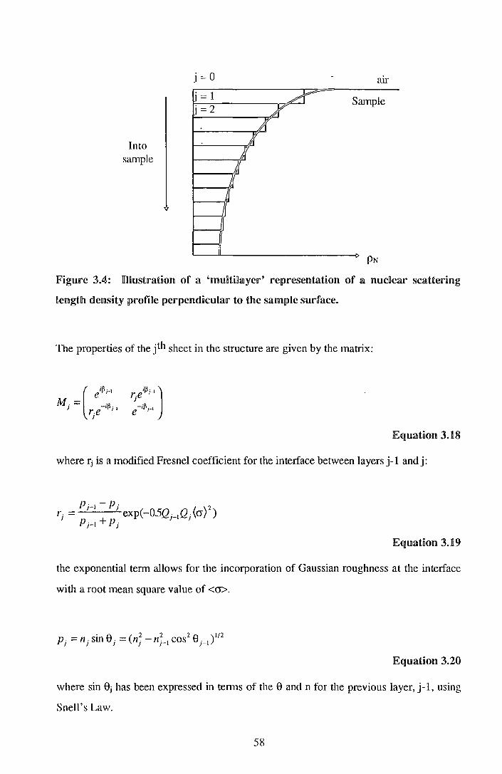
Into sample
i=O
j = 1 j=2
air
Sample
lFfigure 3.4: illllustration of a 'madtillayer' representation of a nuclear scattering
Kell1gtlh density profine perpendicular to the sample surface.
The properties of the jth sheet in the structure are given by the matrix:
Equation 3.18
where ri is a modified Fresnel coefficient for the interface between layers j-1 andj:
Equation 3.19
the exponential term allows for the incorporation of Gaussian roughness at the interface
with a root mean square value of <cr>.
_ . 8 _ < 2 2 2 8 )112 P . - n . sm . - n . - n. 1 cos . 1 1 1 1 1 r r
Equation 3.20
where sin ej has been expressed in tenns of the e and n for the previous layer, j-1, using
Snell's Law.
58

Equation 3.21
nj and Zj are the neutron refractive index and the thickness of the jth layer respectively.
The reflectivity, R, is then given by:
Ecgu.natiorn 3.22
M 11 and M21 are elements of the resultant matrix, MR, obtained as the product of all
the individual matrices for each separate layer, i.e.
Equation 3.23
This system of equations facilitates the extraction of the composition profile via a model
fitting procedure. Figure 3.5 shows some reflectivity profiles for situations that are
typically encountered in this work. The effect of instrument resolution has been included
in these profiles by integrating the reflectivity profile, with no resolution included, over
intervals of the resolution, ~Q, for each data point. Figure 3.5a shows reflectivity
profiles for a series of layers of different thickness, these exhibit 'Kiessig fringes' whose
spacing is inversely proportional to the film thickness. Figure 3.5b shows the effect that
a surface excess of material with higher scattering length density has at the surface of a
film (a two layer profile with a large roughness between the two layers has been used for
these data, the PN at the smface is at a volume fraction equivalent to 0.5 d-PMMA in h
PMMA and the bulk volume fraction is fixed at 0.25, the thickness of the smface excess
layer is varied), these are compared to the reflectivity of uniform films with volume
fractions of 0.25 and 0.5 d-PMMA . Finally, since all samples used in this work were
cast onto silicon oxide substrates which have a layer of native silicon dioxide at the
59
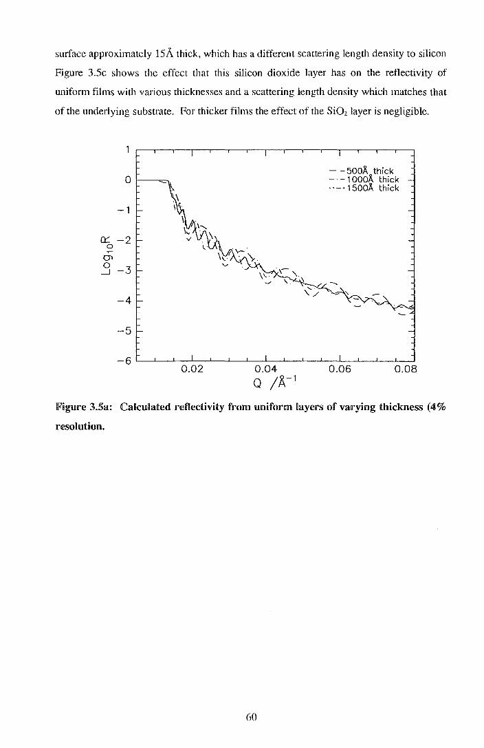
surface approximately 15A thick, which has a different scattering length density to silicon
Figure 3.5c shows the effect that this silicon dioxide layer has on the reflectivity of
unifonn films with vruious thicknesses and a scattering length density which matches that
of the underlying substrate. For thicker films the effect of the Si02 layer is negligible.
0 - - soo..l!.. thick - ·- 1 oooA thick -15001\ thick
-1
0::: -2 0
01 0 -3 _j
-../
-4
-5
-6 0.02 0.04 0.06 0.08
o /A-1
Figure 3.5a: Calculated reflectivity from uniform Bayers of varying thickness (4%
resolution.
60

-1
0:::: -2 0
(J1
0 __j -3
-4
-5
~
'-··. '<··.:.""-. '"' .....
'-... ·· ... .......
0.02
-uniform 0.50 - · · 58)\ excess - · - 33A excess · · · · · · 8)\ excess - -uniform 0.25
--..
0.04 0.06 0.08 Q ;A.-1
!Figure 3.5b: Calculated reflectivity from Dayers with various surface excesses, see
text for detains.
0 -With Si02 layer - -No Si02 layer
-2 0::::
0
(J1
0 __j
-4
-6
0.02 0.04 0.06 0.08 Q ;A.-1
Figure 3.5c: Calculated reflectivity of layers of (top) SOOA and (bottom) 2000A
with and without a 15A Si02 Bayer at the substrate. (2000A data offset by -1 for
cHarity.
61

Even in an ideal world where data can be collected over an infinite Q range with
no resolution effects the- reflectivity, R(Q), is not unique to a single composition profile
because of the loss of phase infonnation 10, furthermore a host of different composition
profiles may all have very similar reflectivity profiles and in a real experimental situation
these profiles will be essentially indistinguishable. On top of this fundamental problem
there is the practical problem of fitting the parameters. Ideally we would like to divide
our model composition profile into a large number of layers so that the model can
accurately represent the composition profile in the sample. Fitting a profile with such a
large number of parameters is difficult and if the usual non-linear least squares methods
are used then a smaller number of parameters are fitted by resorting to the use of
functional fonn models or multilayer models with Gaussian roughness between the layers
where the number of layers is small ( <5).
The preceding paragraph represents the pessimistic side of neutron reflectivity
data analysis, in practice there are reasons to be more optimistic. A substantial subset of
the composition profiles are physically or chemically unreasonable and further to this
additional infonnation can be obtained for the system of interest using techniques which
are sensitive to the surface composition (such as SIMS or XPS) or give a lower
resolution picture of the composition profile (such as NRA) these data can be used to
give starting parameters for the fitting process and discard unreasonable fits.
This section has concentrated on one method of data analysis - the optical matrix
method, which is suitable for the systems studied here. Two further methods are that of
partial structure factors 11 and indirect Fourier transform12 methods. It is also possible to
obtain some infonnation more directly from the reflectivity profile by using the Born or
kinematic approximation which is at the root of the partial structure factor method. The
kinematic approximation is that observed neutrons have undergone only one collision,
i.e. there is no multiple scattering, this approximation breaks done as the region of total
reflection is approached. In the kinematic approximation:
167t 21 I 12 R(Q) =7 2. N(Q)
Equation 3.24
.J;!'N (Q) is the Fourier transfonn of the composition gradients, capN/az), in the sample. In
the limit of large Q, tiN(Q)~:L8(pN(z)), where L{)(pN(z)) is the sum of the 'jumps' in the
62

scattering length density, i.e. at large Q, !).'N(Q) is directly related to abrupt changes in the
scattering length density. Commonly such sharp changes in scattering length density are
only observed at the air I polymer and polymer I substrate interfaces. Fonnally:
R(Q)Q4 = 16n 2 I,(o ( p N (z))) 2
Q~~
Equatnollll 3.25
This means that the air I polymer surface composition of a sample can be obtained
directly from the value of the asymptote of the R(Q)*Q4 vs. Q at large Q, if it can be
arranged that the polymer and substrate have the same scattering length density.
63

3.2 Nuclear Reaction Analysis (NRA)
Nuclear reaction analysis, as applied to polymers, is based on the nuclear
reaction:
Equation 3.26
where Q = 18.352 MeV, the reaction proceeds via the short lived 5Li+. The reaction has
a maximum cross-section at an incident 3He+ energy of 0.7 MeV. The basis of NRA is to
fire 3He + into the partially deuterated sample of interest and measure the energy spectrum
of the resultant 4He (as a particles) or 1H+ (as protons, p). The depth profiling technique
was developed by Dieumegard et a/13 to probe the composition profiles of 2H in silicon.
Only more recently has it been developed by Payne et a/14 and Chaturvedi et a/15 for use
in polymer systems.
Figure 3.6 is a schematic illustration of the NRA experiment, showing the angles
U.~ra and e,lfa, which are the beam I sample angle and the detection angle, respectively.
These angles will influence the depth probed and the resolution.
Figure 3.6: Schematic illustration of the NRA experiment with Unra and 8nra defined
The energies of the resultant p and 4He can be calculated from kinematics, the
situation is illustrated in Figure 3.7. We consider two frames of reference, the laboratory
reference frame (refetTed to using the superscript 'lab') and the centre of mass reference
frame (referred to using the superscript 'em'). The 3He, 4He, 2H and protons (1H) will
64

be refened to using the subsc1ipts 3He, a, D and p respectively. V / and mx will denote
the velocities and masses of the pruticles, respectively.
Figure 3.7: Kinematics ofthe reaction between 3He+ and 2H
In the centre of mass reference frrune the 2H (or D) is no longer stationary but moves
towards the incoming 3He+ with velocity, V0 c111
, such that the net momentum in the
system is zero:
(V I<W V em) V em m3He 3He + D =mD D
m vem 3 . ycm _ 3H,· 3He _ --V'"b • • D - ( ) - 5 3He
m3He +mD
Equation 3.27
After the reaction the net momentum in the centre of mass reference frame is still zero:
m vem = -n1 vem « « I' I'
... 4y~cm = -V em ~ I'
Equation 3.28
This is illustrated schematically in Figure 3.7, the resultant velocities in the
laboratory reference frame are obtained by adding the velocity of the centre of mass,
V0 c111
, to the velocities in the centre of mass reference frame. In the centre of mass frame
of reference the protons will have energy 14.8 MeV and the 4He will have energy 3.7
65

MeV, this means that the signals from the protons, 4He and Rutherford backscattered
3He are all well separated in energy.
As the incident 3He penetrates into the sample it losses energy through electronic
collisions, thus the centre of mass velocity becomes less as the 3He travels deeper into
the sample. This means that protons collected at backward detection angles (8nra>90°)
have an energy in the laboratory reference frame that depends on how deep in the sample
the reaction in which they originated occurred. Protons originating at the surface will
have a lower energy than protons generated deep within the sample. The energy lost by
the proton as it leaves the sample is relatively small, since it travels much faster than the
incident 3He. To maximise the depth resolution the protons should be detected at the
largest Sura available.
NRA experiments have been done on polymers in two modes, with protons
detected at backward angles14 (as was assumed in the discussion above) or with 4He
detected at forward angles 15, in which case 4He or p from the smface have a higher
energy than those from deeper within the sample.
The resolution perpendicular to the sample surface can be improved by tilting the
sample with respect to the incident beam, this increases the path length of the 3He in the
sample for a given depth perpendicular to the surface. Payne et a/14 found a resolution of
300A (Full Width Half Maximum) for samples at 15° to the incident beam and with a
backward detection angle of 165°.
66

3.3 JHtem.oated Total Reflection Dnfrared Spectroscopy (A T!R)
If a material, such as an A TR crystal, is sustaining total intemal reflection then an
evanescent wave will be found 'protruding' from the surface of the matetial. ATR
spectroscopy takes advantage of this by placing the sample of interest in good optical
contact with the A TR crystal such that the evanescent wave penetrates the sample.
Mirabella16 gives a general review of various aspects of total internal reflection
spectroscopy. The notation used here follows that of Fina and Chen17• Total internal
reflection occurs if the angle of incidence§, 8atn is greater than the critical angle, 8c
defined below:
. -1 n,w· ec = sm --nsam
Equation 3.29
where natr is the refractive index of the A TR crystal and nsrun is the refractive index of the
sample placed on the A TR crystal. The intensity of the evanescent wave decays
exponentially away from the smface of the matelial. In the case of zero absorption in the
surrounding medium no energy is radiated away. The intensity of the electric field,
<E .. =2>, in the evanescent wave is given by:
Equation 3.30
where <Eo2> is the electric field intensity at the interface between the ATR crystal and
the sample. dr is the penetration depth, defined below:
A. dp = ----r=2==. =2=8===2=
27t flarr Sln arr - nsam
Equation 3.31
§ The angle of incidence is defined relative to the normal in this section on A TR and relative to the
surface for NR. this is to maintain consistency with the literature.
67

where A is the wavelength of the radiation in free space. Intuitively it can be seen that
the evanescent wave will lead to a depth weighted absorption spectrum of the sample,
with the spectrum dominated by contributions from closest to the crystal surface.
A further parameter, de, is also used in ATR spectroscopy, this is defined as the
thickness of a sample in transmission that would produce the same absorption as the
A TR sample. This is defined by the equation:
nsam(En J ( z } d = exp -- lz e nair cos ea/r 0 d p
Equatiorn 3.32
1/cos Satr is a geometric weighting factor and the term (ns:u,Jnatr)<Eo2> arises because the
intensities of the electric fields in the sample and the A TR crystal are related by the
expression:
Equation 3.33
With a direct analogy to the Beer Law for absorption in the transmission:
Aa,,. = exp(-a~..dJ
Equation 3.34
where Aatr is the measured absorption and Ut.. is the absorption coefficient at wavelength
A, for small aA. the following approximation can be made:
Aatr = 1 - UA.de
Equation 3.35
This is the result of two approximations, that of the exponential term and that of the
exact Fresnel coefficients used in deriving the Beer Law. Combining equations 3.35 and
3.32 gives the equation:
68
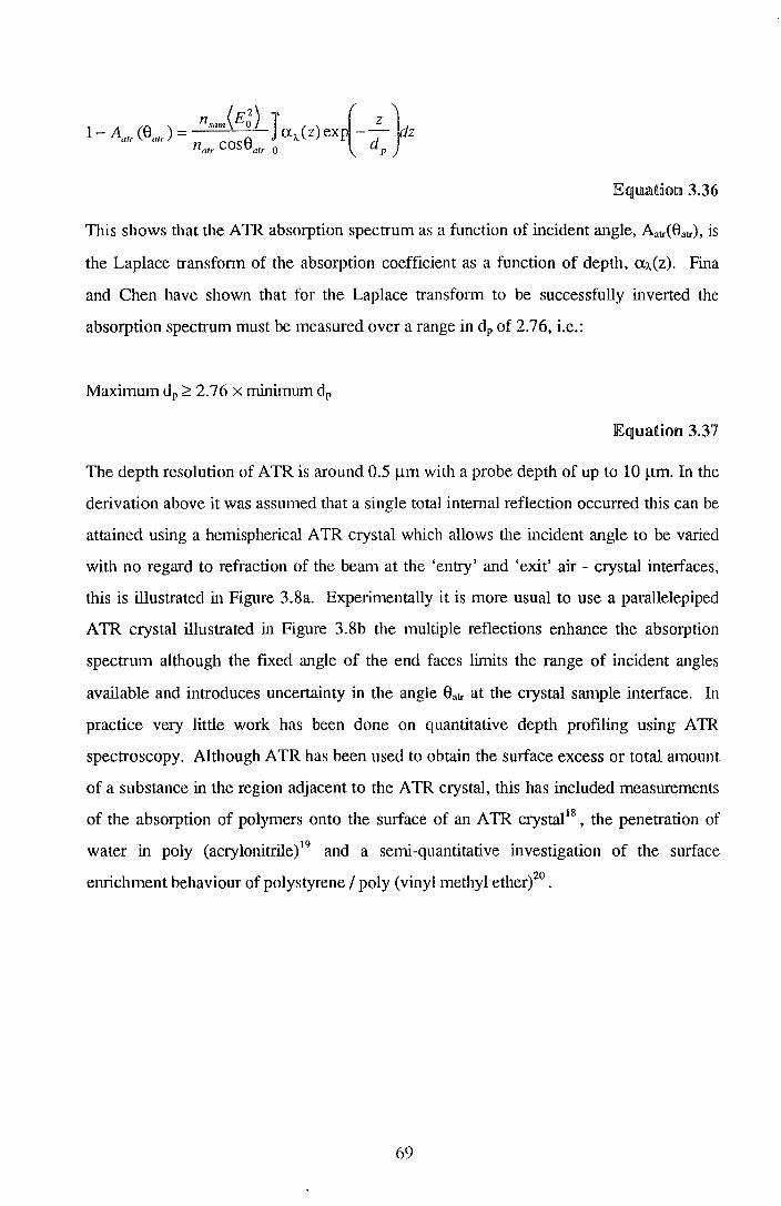
nsam(EJ) J ( ) { Z J / 1- A,1, (8111,) = e a~. z ex - -d cz nair cos atr 0 p
This shows that the A TR absorption spectrum as a function of incident angle, Aatr(Satr), is
the Laplace transform of the absorption coefficient as a function of depth, a~..(z). Fina
and Chen have shown that for the Laplace transform to be successfully inverted the
absorption spectrum must be measured over a range in dr of 2.76, i.e.:
Maximum dr ;::::: 2. 7 6 x minim tun dr
lEquatiorn 3.37
The depth resolution of A TR is around 0.5 f .. .Ltn with a probe depth of up to 10 fJ.m. In the
derivation above it was assumed that a single total internal reflection occun·ed this can be
attained using a hemispherical A TR crystal which allows the incident angle to be varied
with no regard to refraction of the beam at the 'entry' and 'exit' air - crystal interfaces,
this is illustrated in Figure 3.8a. Experimentally it is more usual to use a parallelepiped
A TR crystal illustrated in Figure 3.8b the multiple reflections enhance the absorption
spectrum although the fixed angle of the end faces limits the range of incident angles
available and introduces uncettainty in the angle 8atr at the crystal sample interface. In
practice very little work has been done on quantitative depth proftling using ATR
spectroscopy. Although ATR has been used to obtain the surface excess or total amount
of a substance in the region adjacent to the A TR crystal, this has included measurements
of the absorption of polymers onto the surface of an ATR crystal18, the penetration of
water in poly (acrylonitrile)19 and a semi-quantitative investigation of the surface
enrichment behaviour of polystyrene I poly (vinyl methyl ether)20•
69

(a) ' Sample
(b)
Figure 3.8: Schematic dliagrams of two modes of A 'JI'R spectroscopy
70

3.4 References tor Section 3
1 . J.S. Higgins, H. C. Benoit, 'Polymers and Neutron Scattering', Clarendon Press,
1994.
2. S.W. Lovesey, 'Themy of Neutron Scattering from Condensed Matter, Volume 1 ',
Clru·endon Press, 1986.
3. P.G. de Gennes, 'Scaling Concepts in Polymer Physics', Cornell University Press,
1985.
4. J. Penfold, Rutherford Appleton Laboratory Report, RAL-88-088, 1988.
5 . T.P. Russell, Material Science Reports, 5, ll990, 173.
6 . J. Lekner, 'Theory of Reflection', Martin us Nijhoff Publishers, 1987.
7. M. Born, E. Wolf, 'Principles of Optics 6th ed.', Pergamon, 1980.
8. 0. Heavens, 'Optical Properties of Thin Films', Butterwmth, 1955.
9. J.Penfold, Rutherford Appleton Laboratory Report, RAL-91-023, 1991.
10. D.S. Sivia, W.A. Hamilton, G.S. Smith, Physica B, 173, ll99li, 121.
11 . T.L. Crowley, E.M. Lee, E.A. Simister, R.K. Thomas, Physica B, 173, 199ll, 143.
12 . J. S. Pedersen, Journal of Applied Crystallography, 25, 1992, 129.
13. D. Dieumegard, D. Dubreuil, G. Amsel, Nuclear Instruments and Methods, 166,
].979, 431.
14. R.S. Payne, A.S. Clough, P. Murphy, P.J. Mills, Nuclear Instruments and Methods
B, 42, ll989, 130.
15. U.K. Chaturvedi, U. Steiner, 0. Zak, G. Krausch, G. Schatz, J. Klein, Applied
Physics Letters, 56(13), 1990, 1228.
16. F.M. Mirabella, Applied Spectroscopy Reviews, 21(1&2), 1985, 45.
17. L.J. Fina, G. Chen, Vibrational Spectroscopy, 1, ll991, 353.
18. H.E. Johnson, S. Granick, Macromolecules, 23, 1990, 3367.
19. G.T. Fieldson, T.A. Barbari, Polymer, 34(6), ll993, 1146.
20. J.M.G. Cowie, B.G. Devlin, I.J. McEwan, Macromolecules, 26, 1993, 5628.
71

This page left intentionally blank
72

4J. -u Materials
4U .. n §yntltnesis
All the polymers used in this work were synthesised by F.T. Kiff and the
perdeuterated dibutyl phthalate was synthesised by M. Hartshorne. Outlines of the
synthesis methods used are included here to provide evidence of the provenance of the
polymers used but no expertise in these synthetic methods is claimed. All the deuterated
polymers were prepared by polymerisation of the fully deuterated monomers. In this
work the following abbreviations will be used:
h-PMMA
d-PMMA
h-PEO
d-PEO
h-PS
d-PS
d-PS(F)
d-PS(F2)
h-DBP
d-DBP
hydrogenous poly (methyl methacrylate)
perdeuterated poly (methyl methacrylate)
hydrogenous poly (ethylene oxide)
perdeuterated poly (ethylene oxide)
hydrogenous polystyrene
perdeuterated polystyrene
perdeuterated polystyrene with one end 1H,1H,2H,2H-perfluoro
octyl dimethyl chlorosilane tenninated, this end group will often
be described as 'perfluorohexane' as a short hand.
perdeuterated polystyrene with both ends terminated with
lH, 1H,2H,2H-perfluoro octyl dimethyl chlorosilane.
hydrogenous dibutyl phthalate
perdeuterated dibutyl phthalate
Syndiotactic Poly (methyl methacrylate)
Deuterated and hydrogenous syndiotactic poly (methyl methacrylate) were
prepared by anionic polyme1isation of the purified monomers in tetrahydrofuran solution
73

at 195K using 9-fluorenyllithium as initiator. After tennination by addition of degassed
methanol, the polymers were isolated by precipitation in hot hexane, filtered off washed
and dried under vacuum at 313K for 1 week.
lsotactic Poly (methyl methacrylate)
Deuterated and hydrogenous isotactic poly (methyl methacrylate) were prepared
by the anionic polymelisation of the purified monomers in toluene at 273K using phenyl
magnesium bromide as initiator. After tennination by addition of degassed methanol, the
polymers were isolated by precipitation in chilled hexane. A chilled methanol I HCl
mixture was added to the dried polymer in order to remove magnesium residues from the
initiator. The initial broad molecular weight distribution was narrowed somewhat by re
precipitation.
Poly (ethylene oxide)
Deuterated and hydrogenous poly (ethylene oxide) were prepared by the anionic
polymelisation of the purified monomer in tetrahydrofuran at 340K. The initiator was
diphenyl methyl potassium. The reaction was terminated using degassed ethanoic acid
and the product was then precipitated into hexane, filtered off and dried in a vacuum
oven at 313K.
Polystyrene ((nonnal' andfunctionally end capped)
Deuterated and hydrogenous polystyrene were prepared by anionic
polymerisation of the purified monomer in benzene at room temperature. The initiator
was secondary butyl lithium. To produce 'normal' polystyrene the reaction was
terminated using degassed methanol, the end capped polystyrene was terminated with
1H,1H,2H,2H-perfluoro octyl dimethyl chlorosilane Tllis end capped polymer is
illustrated in Figure 4.1.
74
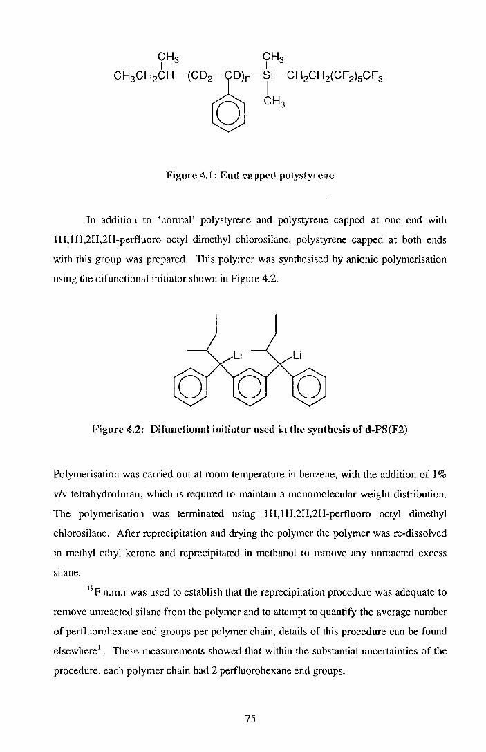
lFfigure <t.li: Eml cajpped polystyrene
In addition to 'normal' polystyrene and polystyrene capped at one end with
1H,1H,2H,2H-perfluoro octyl dimethyl chlorosilane, polystyrene capped at both ends
with this group was prepared. This polymer was synthesised by anionic polymerisation
using the difunctional initiator shown in Figure 4.2.
Figure 4.2: Difunctional initiator used! in the synthesis of dalPS(lF2)
Polymerisation was cruTied out at room temperature in benzene, with the addition of 1%
v/v tetrahydrofuran, which is required to maintain a monomolecular weight distribution.
The polymerisation was terminated using 1H,1H,2H,2H-perfluoro octyl dimethyl
chlorosilane. After reprecipitation and drying the polymer the polymer was re-dissolved
in methyl ethyl ketone and reprecipitated in methanol to remove any unreacted excess
silane. 19F n.m.r was used to establish that the reprecipitation procedure was adequate to
remove unreacted silane from the polymer and to attempt to quantify the average number
of perfluorohexane end groups per polymer chain, details of this procedure can be found
elsewhere1• These measurements showed that within the substantial uncertainties of the
procedure, each polymer chain had 2 perfluorohexane end groups.
75
Dibutyl phthalate
Hydrogenous dibutyl phthalate was purchased from Aldrich Chemical Company
Ltd, Gillingham, Dorset. Perdeuterated dibutyl phthalate was synthesised by M.
Hartshorne at Strathclyde University. Both compounds were used as received.
~.R.2 MoRectdar weights and! distributions
The molecular weights and disuibutions of the polymers produced were
detennined by size exclusion chromatography, the eluting solvent was CHCh, in all cases
the calibration was by polystyrene standards. The results of these analyses are
summarised in Table 4.1. The codes used in this table will be referred to as 'global
codes', and will be used to indicate which polymers were used at the beginning of each
results and discussion section. These codes are the original codes used to designate
these polymers at Durham.
76

Polymer Code - Mw Mw/Mn
syndiotactic h-PMMA TK21 994,000 1.3
TK76 148,000 1.3
syndiotactic d-PMMA TK24 12,400 1.2
TK20 17,900 1.1
TK25 25,200 1.1
TK22 118,000 1.2
TK26 136,000 1.1
TK23 417,000 1.3
isotactic h-PMMA TK118 322,000 9.4
isotactic d-PMMA TK120 65,500 9.1
h-PEO TK74 124,000 1.1
d-PEO TK77 102,000 1.2
h-PS TK79 44,700 1.1
TK58 1,710,000 1.2
TK85 891,000 1.2
TK45* 87,000 1.0
49% d-PS/h-PS copolymer TK47* 80,000 1.0
d-PS TK48* 86,000 1.0
TK93 816,000 1.7
d-PS(F) TK89 31,700 1.1
TK92 658,000 1.1
d-PS(F2) TK145 56,000 1.0
*eluting solvent tetrahydrofuran.
Tabne 4.1: Molecular weights and distributions of polymers used!.
77
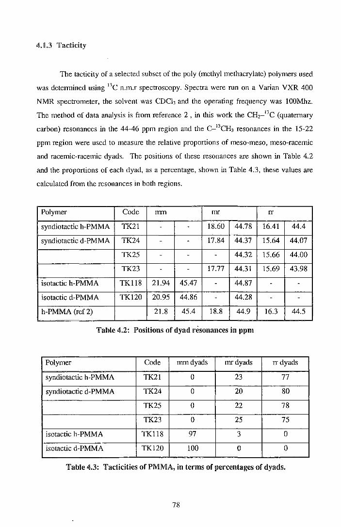
ta.li.3 'lfactndty
The tacticity of a selected subset of the poly (methyl methacrylate) polymers used
was detennined using 13C n.m.r spectroscopy. Spectra were run on a Varian VXR 400
NMR spectrometer, the solvent was CDCh and the operating frequency was lOOMhz.
The method of data analysis is from reference 2, in this work the CH2-13C (quaternary
carbon) resonances in the 44-46 ppm region and the C-13CH3 resonances in the 15-22
ppm region were used to measure the relative proportions of meso-meso, meso-racemic
and racemic-racemic dyads. The positions of these resonances are shown in Table 4.2
and the proportions of each dyad, as a percentage, shown in Table 4.3, these values are
calculated from the resonances in both regions.
Polymer Code nnn till IT
syndiotactic h-PMMA TK21 - - 18.60 44.78 16.41 44.4
syndiotactic d-PMMA TK24 - - 17.84 44.37 15.64 44.07
TK25 - - - 44.32 15.66 44.00
TK23 - - 17.77 44.31 15.69 43.98
isotactic h-PMMA TK118 21.94 45.47 - 44.87 - -
isotactic d-PMMA TK120 20.95 44.86 - 44.28 - -
h-PMMA (ref 2) 21.8 45.4 18.8 44.9 16.3 44.5
Table 4.2: Positions of dyad resonances in ppm
Polymer Code mmdyads tmdyads IT dyads
syndiotactic h-PMMA TK21 0 23 77
syndiotactic d-PMMA TK24 0 20 80
TK25 0 22 78
TK23 0 25 75
isotactic h-PMMA TK118 97 3 0
isotactic d-PMMA TK120 100 0 0
'fabne 4.3: 'facti cities of PMMA, in terms of percentages of dyads.
78

4.2 Small Angle Neufron Scauering (SANS)
~.2.li S3mplle 1Prepar31non
For the SANS work plaques of the polymer mixture 12mm in diameter and
approximately lmm thick were required. These were prepared by, fust, co-dissolving
the appropriate polymers in an approximately 5% total weight polymer solution. This
solution was then poured slowly into a non-solvent (either chilled methanol or hexane),
the resulting precipitate was then filtered off using a sintered glass filter and a Buchner
flask. The precipitate was washed with the non-solvent and allowed to dry in air at room
temperature. Final drying was for 2 days under vacuum at 313K. Plaques were made
from the mixtures prepared in this way using a heated Specac Infrared press, the
appropriate weight of the polymer mixture to be used was placed between the die plates
of the press. Typically a pressure of 2 tonnes was then applied and the temperature of
the die increased to 453K, in the early compression stage a vacuum was applied to the
die although in the later compression stage no vacuum was applied. The die was held at
453K for approximately one hour then it was allowed to cool, this took around 1.5
hours, then the resulting plaque was removed from the die. The plaques were unifonn in
thickness and free of macroscopic air bubbles, when prepared. The thickness of the
samples was detennined using the average of three micrometer readings and the plaques
were then placed in cylindrical brass and ahuninium cells with quartz windows
approximately lnun thick.
4.2.2 ILOQ
All the Small Angle Neutron Scattering (SANS) data presented in this work were
collected using the LOQ diffractometer at ISIS, Rutherford Appleton Laboratory,
Chilton, near Oxford. Figure 4.3 is a schematic diagram of LOQ. The diffractometer
views the liquid hydrogen moderator which is at 22K.
79

-·:
Figure 4.3: Schematic diagram of LOQ, side elevation. Key to symbols in text.
(Not to scale)
The LOQ disc chopper (C) operates at 25Hz, i.e. selecting alternate pulses of neutrons
from the target, this provides a useful wavelength range of 2.0-9.8A. The neutrons are
collimated by three apertures (sl, s2, s3) producing a beam at the sample (X) 8mm in
diameter. Frame overlap mirrors (0) remove long wavelength neutrons (> 13.7 A) which
would otherwise interfere with neutrons from preceding pulses. The Soller bending
mirror (S) deflects all but the shortest wavelength neutrons, this means that the detector
(D) does not have a direct 'view' of the source and reduces the background radiation.
The available Q range on LOQ is 0.006A-1 to 0.22A-1, limited by the size of the beam
stop at low Q and the size of the detector at high Q. The neutron flight path from the
source to the sample position and from the sample position to the detector is evacuated
to minimise neutron losses through air scattering, although the sample position itself is
typically under ambient conditions. Neutrons scattered from the sample are detected by
a 3He-CF4 filled area detector 64cmx64cm, this is encoded as 128x128 pixels. The
detector is arranged such that the direct beam falls in the middle of the detector. The
vacuum tank and the detector are heavily shielded to reduce background.
Samples were placed in an eight position, temperature controlled sample rack
driven by the LOQ CAMAC electronics. The temperature of the rack was monitored by
a single thermocouple at the centre of the rack. At the temperatures used in this work
the thermocouple shows the rack temperature fluctuating in a regular sinusoid with a
petiod of ~5 minutes and an amplitude ±3K, the mid point of this range is within 0.5K of
the temperature set. The positions on the sample rack were aligned using a laser
coincident with the neutron beam. Rack position, rack temperature and sample
80

'exposure' time can be controlled automatically using a command file on the LOQ front
end computer.
For each sample run at each temperature two measurements are made, firstly the
transmission of the sample as a function of wavelength is measured by applying a small
collimation aperture to the incident beam, and placing a scintillation monitor immediately
after the sample position. The sample transmission can be calculated given this
measurement and a similar measurement of the 'direct beam' with no sample in place.
Secondly the total small angle neutron scattering, I,o,(S,<j>,A), is measured using the area
detector. Where 28 is the scattering angle from the direct beam, <1> is the azimuthal angle
and A is the neutron wavelength. The raw scattering data is corrected for incident beam
flux, detector efficiency and sample transmission, in addition the data were converted
from 11o1(8,<j>,A) to I,o,(Q, <j>) where Q = (4n/A)sin 8. Finally because the data were
azimuthally isotropic I10,(Q, <!>) was azimuthally averaged to give I10,(Q). All these
procedures were carried out at the Rutherford Appleton Laboratory using the
COLLETTE program. The output from COLLETTE is nominally in absolute intensity
units (cm-1), but as a further calibration procedure blends of d-PS/h-PS were run at room
temperature on each occasion that LOQ was used. This calibration will be discussed
further in the next section.
41.2.3 Calibration
The absolute calibration of the Small Angle Neutron Scattering is important if
accurate values of x are to be obtained, in principle data from LOQ is in absolute units3 ,
but as a further calibration procedure a d-PS/h-PS blend with 0.47 volume fraction of d
PS was run on each occasion that scattering data were collected. Polymer blends have
been used previously for the calibration of SANS4 •5
, principally because they exhibit
very strong scattering at low Q, this is important because it minimises the time required
to make the calibration measurement. For the calibration procedure in this work two
samples were run at room temperature, a blend containing 0.47 volume fraction d-PS in
h-PS and a random copolymer of h-PS and d-PS with the same volume fraction of d-PS
as the blend. The copolymer is run in order to measure the background scatter· for the
blend, background subtraction is discussed in the next Section 4.2.4. The molecular
weights of the polymers used were measured by size exclusion chromatography (SEC)
81

with either chloroform (CHCh) or tetrahydrofuran (THF) as the eluting solvent, these
values are shown in Table 4.4, along with values of the degree of polymerisation, N,
calculated from these weights.
Solvent Mw Mw/l\.1n N
h-PS CHCh 73,500 1.1 710
CHCh 77,050 1.1 740
CHCb 80,350 1.1 770
THF 86,900 1.0 835
d-PS CHCh 71,100 1.1 635
THF 86,200 1.0 770
Table .:3.41: Molecular weights of poRymers used in calibration
There is a fairly large variation in the molecular weights detennined in this manner, this
will be discussed later. After background subtraction, the scattering was fitted using the
Random Phase Approximation (see Section 2.1). Polystyrene is known to scatter in an
ideal manner according to the Debye function6• The constants used were as follows: bH
= 2.328x10⁻¹² em-', bo = 10.660xl0-12 em-', the average value of the segmental volume7,
V = 1.725x10⁻²² cm-3 , the average degree of polymelisation N = 800, X was fixed at
zero. The data were fitted using the FORTRAN program BANTAM (listing in
Appendix 10.4) which is based on the interactive fitting library FITFUN, statistical error
weighting was used. The radii of gyration of the two polymers were allowed to vary but
the constraint RgH = Rgo was applied. Figure 4.4 shows a representative fit to the data,
there are small deviations from the ideal scattering at high Q. This may be due to a slight
over subtraction of the background scatter. Table 4.5 shows values of the normalisation
constant, kN, and Rg (= RgH, Rgn) fitted to the calibration sample on the four occasions on
which the SANS data were collected.
82

100
+ Data -fit
80
~
I 60 E
()
"---....---....
40 0 '---/
20
0.05 0.10 0.15 0.20 Q ;A.-1
!Figure 4!.41: !Fnt to the JuRy li993 caHibratimu sampne llisnng the lRamllom JP!hase
Approximation. lError lbars from Poisson statnstics.
Rg/A kN
September 1992 68.8(2) 0.940(3)
December 1992 68.3(2) 0.841(3)
June 1993 72.5(2) 0.948(3)
July 1993 71.1(2) 0.952(3)
Table 4.5: Values fitted for the radlii of gyration and tlhe normalBsatnon constant
The nonnalisation constant, kN, is the amount by which the model function must
be multiplied in order to fit the data - the data must be multiplied by 1/kN to convert to
absolute units. Figure 4.5 shows the scattering from the calibration sample runs in the
Kratky mode following multiplication by the normalisation factor (1/kN), Figure 4.6 is a
detail of the low Q region. These data are, in ptinciple, on an absolute scale and so
should be identical. The overlap at low Q is good, but at higher Q values (0.05A-1 to
0.1 OA-1 there are discrepancies. There is a difference between data collected in 1992 and
that collected in 1993, this is probably due to an adjustment of the detector electronics
between the end of 1992 and mid-1993.
83

0.030
~
I 0.025 E u
N 0.020 I
0<( ~ 0 0.015
* 0 o.o1o
0.005
0.05
0 September 1992 6. December 1992 + June 1993 x July 1993
0.10 0.15 Q ;A.-1
0.20
Figure ~.5: Kratlky pBots of data coll!ectedllfrrom callilbration samplles and normalised
by calibration constant
I
E
0. 0 2 5 .--..,.--.------y-,.---,l,-..,.----,-----y-,.---,1;---,----,-----y-,.--,
0.020 - 0 September 1 992 6. December 1992 + June 1993 x July 1993
-
() 0.015-N I
0<( ~ r-... 0 0.010- -
* N
0 0.005- -
0. 000 '---_..j____...____._~-'---l_.____.____._.....__--'1'--...._____.____.._....._____. 0.005 0.010 0.015 0.020
Figure 4.6: DetaiB of Figlllre 4.§ (above) showing the low Q region of the Kratlky
plots.
84

There are several sources of error in this calibration procedure: the uncettainty in
the molecular weights of the polymers and hence inN, the influence of non-zero X values
and the uncertainty in the density and hence the segmental volume and the possibility that
the copolymer is not a sufficiently good measure of the background scatter. Segmental
volumes for d-PS and h-PS were calculated from values for the density of d-PS and h-PS
in Russell7 (a general review of neutron reflectometry). Davidson8 has measured values
for the density of h-PS and d-PS, the average value for the segmental volume is lower
(1.653xl0-22 cm3 compared to 1.725x10⁻²² em\ Davidson's value for the density of h
PS is in agreement with the value for h-PS in Brandrup and Immergut9 • This difference
in segmental volumes results in a 4% reduction in the fitted value of kN.
The N used were the average of values obtained using THF SEC, using the
average of NH and Nn makes a small difference to the value of kN fitted, but values of N
obtained using the CHCh SEC are rather lower than those measured by THF SEC.
Using the average of the values obtained using CHCh SEC to calculate N produces a
20% increase in the fitted value of kN. Finally there is the influence of X on the fitted
value of kN, Wignall et at states that the influence of X on the scattering from low
molecular weight polymers is negligible, thus X was initially set to zero. However, if X is
fixed at values indicated by Bates et a/10 then values of kN fitted are up to 10% lower
than for X= 0, the normalised X2 parameter is slightly lower for X'* 0 than for X = 0.
Table 4.6 is a compendium of kN values that have been obtained by fitting the data from
the July 1993 calibration measurements.
NH Nn Rg/A V /cm3 X kN ·x2/Np'
1 800 800 71.1 1.725x10⁻²² 0 0.952 2.12
2 835 770 71.1 1.725x10⁻²² 0 0.989 2.12
3 835 770 71.2 1.653xl0-22 0 0_948 2.12
4 740 635 71.1 1.653xl0-22 0 1.149 2.12
5 740 635 69.5 1.653x10⁻²² 1.6xl04 1.092 2.12
6 740 635 68.9 1.653xl0-22 2.1xl04 1.074 2.09
7 740 635 67.3 1.653xl0-22 3.7xl04 1.016 2.06
Table 4.6: ComiPen<llium of fitted lkN values. Average value of kN = 1.03(7)
85
Items 1 and 2 in this table show the effect of averaging N1-1 and N0 , 2 and 3 show the
effect of using values of V calculated from Davidson rather than Russell, 3 and 4 show
the effect of using values of NH and No from CHCb rather than THF SEC and finally
items 4-7 show the effect of non-zero values of X· The values of X are those calculated
at the measurement temperature (2.lxl04) and the temperatures at which the sample
was pressed (3.7x10⁴). 'X21Nr' is the nonnalised X2 parameter of the fit, the values in
this table represent good fits.
The conclusion from this calibration work is that uncertainty in the molecular
weights of the polystyrenes used in the calibration sample limit the accuracy of the
calibration procedure to ±10%, this accuracy could be improved by measuring the
molecular weight of the polymers using light scattering and by running this calibration
sample on other neutron sources. Despite the uncertainty in the absolute accuracy of the
calibration procedure all the data in this thesis should be on the same relative scale.
86

~.2A lBaclkgmwndl Su.nbtmctnorn
The scattering function of interest in this work is the elastic coherent scattering,
I(Q), of the polymer blend. What was initially measured was the total scattering of the
sample and the sample cell which is a sum of elastic coherent, elastic incoherent, and
inelastic incoherent scattering from the sample and the sample cell. The sum of all of the
scattering that is not elastic coherent scattering will be referred to as the 'background'
scatter. To correct for the background scatter pure hydrogenous and pure deuterated
samples of the polymers in each blend were run at each temperature at which the blends
were run. A weighted sum of the scattering from the pure components was made such
that it matched the composition of the blend. These pure polymers produce no elastic
coherent scattering but will provide a measure of all the incoherent and inelastic
processes that the blend exhibits. Subtraction of the sample cell scattering is implicit
because both blend and pure polymer samples are held in identical cells and the weighted
sum of scattering from the pure polymers will contain contributions from the equivalent
of one sample cell. Figure 4. 7 shows representative scattering from various pure
hydrogenous and deuterated polymers and the scatter from a sample cell.
1.5
I
E u
"'-.. 1 .0
0.5
0.05 0.10 0.15 0.20 Q ;A.-1
JFigure 4.7: Scattering from pure hydrogenous and dleuterated ponymers, and the
empty sample cell.
87

It is clear that the background scattering arises substantially from the hydrogenous
polymers, this is due to the much larger incoherent scattering power of hydrogen
compared to deuterium. This method of background subtraction has been used
extensively in SANS work of this type. Comparisons of the scattering from pure
hydrogenous polymers with scattering predicted solely from the bound atom incoherent
scattering cross-sections of the constituent atoms show that there are considerable
contributions to the background scattering from inelastic processes. This has been
commented on in the literature11 '12
'13
, these inelastic processes cannot be evaluated
theoretically and so an a priori calculation of the background scattering is not possible.
41.2.5 J[)ata Aum!ysis Methods
The equations used to analyse the Small Angle Neutron Scattering (SANS) were
presented in Section 2.1, in this section the 'mechanics' of the fitting process are
described. A series of FORTRAN programs were written to perform non-linear least
squares to the scattering data, using the Random Phase Approximation. These programs
were based on the FITFUN14 interactive fitting routine, which uses a Marquardt -
Levenson15 fitting algorithm, in this work the fit was weighted by the error in I(Q). Four
programs were used in the analysis of the scattering data:
Pullet
Pullet2
Pullet3
Pullet4
the most basic version, which assumes that both blend components are
monodisperse and have equal segment volumes, V.
mondisperse blend components with different segment volumes.
blend components with a Schultz - Zimm distribution of molecular
weights and different segment volumes.
monodisperse blend components with different segment volumes and a
residual background.
Listings of these programs are in Appendix 10.4. All the programs display the data in
Kratky form, Q2I(Q) vs Q, in this form the differences between the fit and the data are
more apparent, particularly at higher Q. Values for the volume fraction of deuterated
polymer, <j>, degrees of polymerisation, N;, segment volumes, V;, and scattering lengths,
b;. were all fixed. Values for V; were calculated from literature values for the polymer
densities (see Table 4.7), values for the nuclear scattering length were calculated from
the literature, values of N; were calculated from the weight average moleculm· weight of
88

the polymers (measured by size exclusion chromatography) and the monomer masses. It
was assumed that there was no volume change on deuteration. RgH, Rgo and X were
fitted, after an initial attempt the 'step size', i.e. the amount by which parameters were
varied during each iteration of the fit, was reduced. FITFUN generates estimates of the
uncertainty in the fitted parameters, based on the shape of the local fitting minimum. It
was found that X rapidly reached a well defined value, i.e. with a small uncertainty, the
radii of gyration of the blend components were fitted rather poorly because the scattering
is sensitive to the combination of the radii of gyration rather than the individual values.
Straight line fits to the Ornstein - Zernike plot were carried out using
GENPLOT16• No statistical error weighting was used, so the points at low Q where the
error due to the subtraction of the direct beam is large were excluded from the fit.
Polymer Scattering length /cm-1 Segment volume /cm3
isotactic d-PMMA 3 9.821xl0"12 c1.359xl0-22
isotactic h-PMMA 3 1.493xl0"12 c1.361x10-22
syndiotactic d-PMMA 39.821x10"12 d1.446xl0-22
syndiotactic h-PMMA 3 1.493xl0"12 d1.444xl0-22
d-PEO b4.58xl0-12 e0.716x10"22
h-PEO b0.41xl o-12 e0.718xl0-22
Table 4.7: Segment volumes, V~, and scattering lengths, bb of the polymers used in
this work. Values from (a) T.P. Russell, Material Science Reports, 5, (1990), 171, (b)
J.R. Henderson, PhD Thesis, 1992, (c) 'Polymer Handbook 3rd edition pp V/19', J.
Brandrup, E.H. Immergut, John Wiley & Sons, 1989. (d) ibid, V/77, (e) S.
Cimmino, E. Martesculli, C. Silvestre, Polymer, 30, (1989), 393.
89

4.3 Neutron !Reflectometry
4!.3.R §amjpne JPrejparatnon
Thin film samples for neutron reflectometry and nuclear reaction analysis were
prepared by spin casting. In both cases polished silicon substrates were used with
orientations <100> and <110>, no attempt was made to remove the silicon oxide layer
that is found on such substrates. Substrates for neutron reflectometry were disks 50mm
in diameter and Smm thick, for the nuclear reaction analysis similar disks 1.25mm thick
were used. The silicon was used as received or if re-used the following cleaning
procedure was applied: washing in chloroform followed by wiping using optical tissue,
soaking overnight in AR toluene followed by 15 minutes in an ultrasound bath, whilst
immersed in fresh toluene, and a final wipe with optical tissue.
Spin casting was done using a Dynapert Precima Ltd photoresist spinner. An
aliquot of the required polymer solution was placed on the silicon substrate, typically
circa 0.5cm3 was used and this covered 75% of the polished surface, the substrate was
immediately spun for 30-60 seconds. The thickness of films prepared in this way can be
controlled by varying the concentration of the casting solution or the spinning speed. It
was found that varying the casting solution concentration was the more flexible method
of controlling the film thickness. A discussion of the film formation process during spin
casting can be found in reference 17 .
After spin casting all but the dibutyl phthalate/polystyrene films were allowed to
dry overnight under vacuum at room temperature. Any annealing procedure was further
to this initial treatment.
The thicknesses of films were measured using contact profilometry. This is a
mechanical measurement achieved by measuring the displacement of a stylus as it is
drawn across small scratches made in the film, exposing the substrate. The precision of
this technique is of the order of 50 to 100A.
90

4.3.2 CllUSl?
All the neutron reflectometry results presented in this work were carried out
using the CRISP reflectometer on the ISIS pulsed neuu·on source at the Rutherford
Appleton Laboratory. The aim of the neutron reflectometry experiment is to measure
the neutron reflectivity, R, as a function of the scattering vector Q where:
4rc . Q=-sm8
A
and
Equation 4.1
Equation 4.2
where A is the neuu·on wavelength and 28 is the scattering angle ( the angle between the
plane of the sample and the incident beam is 8). Ir is the reflected intensity and Io is the
incident intensity of the neutron beam. CRISP is a variable wavelength instrument,
where the principle method of covering the Q range is by variation of A.
Figure 4.8 is a schematic of the CRISP instrument. Neutrons travel from the
moderator, which lies to the left of the region shown in this figure through the sample
position (X) to the detector (D) on the right. CRISP uses neutrons from the hydrogen
moderator and utilises every pulse generated (i.e. has an operating frequency of 50Hz).
The disc chopper (C) selects a wavelength range circa 2A - 6.4A. This gives the Q
ranges shown in Table 4.8, for the incident angles 8 of 0.25°, 0.6° and 1.2° used in this
work.
91

!Figure 4.8: §ctnematnc mustration of CIR.ll§IP, SRde elevatiollll. IKey to symlboRs ns fin
text
Incident Angle (8/2) o I
Q/A- range
0.25° 0.009 0.027
0.60° 0.021 0.065
1.20° 0.041 0.132
'falbUe 41.8: Q ranges prolbed by Cl!USIP using various n~rnddent ~mgHes.
The neutron beam is crudely collimated between the moderator and the region shown in
this figure. It is subsequently collimated more fmely by slits, s1 and s2, the aperture
height of these slits determines the geometric resolution, 11Q/Q, given by the equation
below:
lEquation 4.3
s1 and s2 are the heights of the two collimation slits, ds is the sample to detector distance
and e is the incident angle. The slit widths are generally fixed at 30mm, these widths do
not effect the resolution in Q. The collimated neutrons are reflected from the sample at
X and then pass through further slits, s3, and the funnel, F, to the detector which is either
a single detector or a 1-dimenional multidetector.
92

The function of the funnel, which is covered in boron impregnated resin - a
strong absorber of neutrons - is to reduce the level of background radiation impinging on
the detector. The detectors are also heavily shielded with boron impregnated resin. A
number of other measures are taken to reduce background count rates; when the protons
strike the tantalum or uranium target a pulse of high energy neutrons and y-rays is
produced, a proportion of the neutrons are not moderated and these along with the y
rays, will contribute to the background. The nimonic chopper, N, is timed such that it
blocks the view of the target during the period of the proton pulse and the supermirror,
S, will reflect neutrons in the useful wavelength range but high energy neutrons and y
rays will pass straight through. This means that the sample position and detectors are
offset from a direct line view of the target and a major source of background counts.
The frame overlap mirrors, 0, reflect long wavelength (slow) neutrons originating from
previous pulses, the shorter wavelength pass straight through. In addition to these
measures further procedures in the data analysis are used to measure background counts
and correct for them in the output data.
The beam monitor, M, is used to measure the incident beam flux, 10 , this and a
further beam monitor are also used for diagnostic purposes to ensure useable neutrons
are reaching the sample position.
The function of the sample position is to present the samples to the neutron beam
at the appropriate angle, in addition provision for the automatic changing can be made.
Since the samples used here are reflective to light the sample is aligned with a laser
coincident with the neutron beam. In this work the sample position was used in two
configurations:
(1) Single sample, (automatic) angle control.
(2) Multiple sample, manual angle control.
In the frrst configuration a single sample is run at all the required incident angles
and the sample is then changed manually. The second configuration is a four position
sample changer which moves the samples horizontally and perpendicular to the neutron
beam. The samples are attached, by suction, to four separate manual goniometers. The
four samples are aligned and can then be run in sequence under automatic control. Some
problems were experienced with the goniometers shifting during movement of the sample
rack, this is particularly worrying when the single detector is used because if the sample
angle changes the specularly reflected beam misses the detector.
93
Two detectors are available for use on CRISP:
(1) 1 dimensional position sensitive multidetector, this is a BF3 gas filled detector with a
sensitive area 250mm high, this area is encoded as horizontal strips with a spatial
resolution of around lnun. The advantages of the multidetector are that it is flexible -
able to measure specular and off specular reflectivity in a single measurement and the
alignment is less demanding since there is a large detector area to aim at and the position
of the specular reflection can be detennined precisely. The background level can be
measured quickly and directly from the signal collected away from the specular peak in
the plane of the detector.
(2) Single detector, this is a single scintillation detector element providing no
information on the vettical position of the detected neutrons. The single detector is used
with additional slits, s4, immediately before the detector position. The advantage of the
single detector is that it has a higher sensitivity and lower intrinsic background than the
multidetector.
For this work the preference was to use the multidetector, however this is not a
critical decision since the specular reflectivity, R, is identical regardless of the detector.
On each occasion that experiments were done a direct beam measurement was
made in order to provide a reference position for detennining the angle of reflection.
Data were then obtained for each sample in tenns of counts versus time (for the single
detector or counts versus (time, position) for the multidetector. Where the time is the
time of the last proton pulse and is directly related to the wavelength of the detected
neutron. The initial data reduction was carried out using a suite of programs in the
GENIE environment. Single detector data was reduced in a single step to un-normalised
R(Q) using the program @g:norm which corrects for detector efficiency and incident
beam flux, as measured by the beam monitor, M. Multidetector data was reduced in a
two stage process, firstly a plot of total counts versus position on the multidetector, x,
was obtained using @g:multidet. A typical example of such a plot is shown in Figure
4.9. The exact angle of incidence was calculated from the centre of the specular peak,
which is found either by eye or using a Gaussian peak fitting routine. The second stage
of the reduction was done using the program @g:nonn_md2. The reflectivity, R, at each
value of Q was obtained by integrating over x. At this point a background subtraction
can be made by assmning that the background under the specular peak can be obtained
by interpolating the background level either side of the specular peak and subtracting this
from the specular peak.
94

6
5
>, ~4 en c Q)
-~--'3 c
2
1
Specular peak
Background
110 120 130 140 150
Position /mm
!Figure .:8.9: 'JI'ypical o8.lltput. frrom the program @g:mu.dtndlet of totan lllleu.ntron
intensity versus position on neutron detector, showing the specular reflection peak
and some background counts.
Using either the single or multidetector, data was produced in the fonn of up to
three separate datasets per sample of R(Q), covering different overlapping Q ranges,
arising from the different incident angles. This is illustrated in Figure 4.10.
The reflectivity, R, may be on different scales, and this scale will not be an
absolute scale. Nonnalisation was carried out by multiplying the data collected at the
lowest angle by a factor such that the reflectivity in the region of total reflection,
observed for all the samples in this work, is one. Data collected at higher angles were
normalised by eye to this lowest angle dataset using the region of overlap.
After nonnalisation the data from different incident angles were 'rebinned' into
the same Q interval and Q resolution and then combined into a single dataset using either
the program @g:combine or the program WELDER written at Durham. @g:combine
will crash if there are negative values of R in any of the datasets to be combined,
negative values of R arise in multidetector detector at high Q values where there may be
slight over-subtraction of the background.
95

0
0::: -2 0
CJl 0 _j -4
-6
0.02 0.04 0.06 a /A-1
0 0.25° data .6. 0.60° data + 1.2° data
+ +
0.08 0.10
lFigure 41.10: JRe1fllectivity data coRRected from the same sampHe at three dlnfferernt
in"ncidernt aHllgles. 0.25° data normalnsecll to ll nHll regnoHll of total refllectnvity, otltner data
un-normanised.
If the single detector was used then the reflectivity was measured up to a Q value
where R is independent of Q. This value is taken to be the background level and is then
subtracted from the whole Q range. For the samples used here the background for the
single detector was very small and the subtraction of this background had little effect on
the fitted composition profile.
The result of this data reduction was to produce a single file of R(Q) data, with
errors in R calculated from Poisson statistics, for each sample run. Before continuing
two comments will be made:
(1) For the purposes of combining data collected at different angles the presence of
Kiessig fringes in the reflectivity can be very useful because they provide a rigorous
check on the incident angles e used in the data analysis, if the values are wrong then
there will be a mismatch in the fringes in the overlap regions.
(2) Throughout this work data collected at different angles has been combined to fonn
one large dataset. There may be some merit in keeping the data collected at different
angles separate and analysing the separate datasets as a group.
96

41.3.3 Data Analysis Methods
The principles by which the neutron reflectivity of a model profile can be
calculated were outlined in Section 3.1.2. Model composition profiles were fitted to the
reflectivity data using two methods:
(1) The FORTRAN program PHOENIX, written at Durham. PHOENIX utilises the
FITFUN14 routine, which is itself based on a Marquardt-Levenson 15 algorithm. A listing
of this program can be found in Appendix 10.4. The program includes multilayer
models, with Gaussian roughness, for up to 4 layers, in addition there are also functional
fonn models based on the modified exponential function:
lEquation ~A
and a Tanh profile:
lEquation .:a.s
Where ~(z) is the volume fraction of the deuterated component as a function of
depth, z, from the air- polymer interface. These profiles are approximated using layers
of equal thickness - generally 15A thick -although this thickness is under user controL
These functional fonn profiles can be placed either at the air - polymer, polymer
substrate or both interfaces. Resolution effects are accounted for by convoluting the
model reflectivity with a box function of the appropriate width. PHOENIX uses the Fit
Index (F.I) as the measure of the fit quality. The Fit Index is given by:
Equation ~.6
97
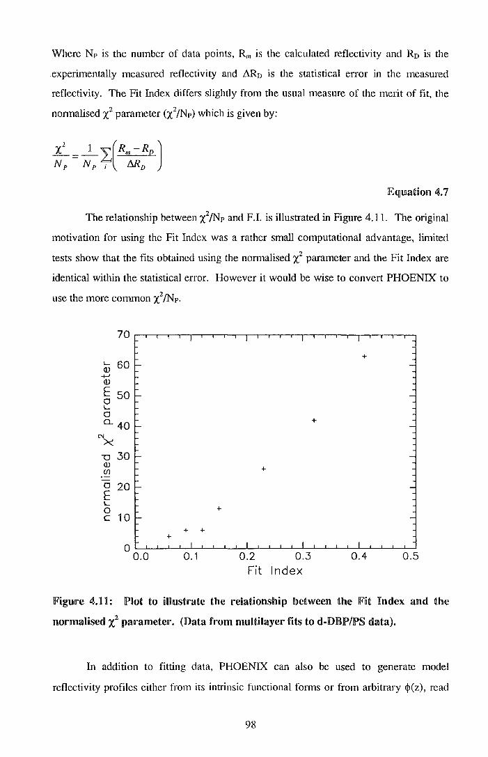
Where Np is the number of data points, Rm is the calculated reflectivity and R0 is the
experimentally measured reflectivity and ~Ro is the statistical error in the measured
reflectivity. The Fit Index differs slightly from the usual measure of the merit of fit, the
normalised X2 parameter (X2/Np) which is given by:
Equ.natiollll 4.7
The relationship between X2/Np and F.l. is illustrated in Figure 4.11. The original
motivation for using the Fit Index was a rather small computational advantage, limited
tests show that the fits obtained using the nonnalised X2 parameter and the Fit Index are
identical within the statistical error. However it would be wise to convert PHOENIX to
use the more common X2/Np.
L 60 (J)
+-' (1.)
E so 0 L
0 0... 40
N>< "'0 30 (J) (fJ
0 20 E L 0 c 10
0
+ +
0.0 0.1
+
+
+
+
+
0.2 0.3 0.4 0.5 Fit Index
Figuure 4l.U: IPBot to mustrate the reBatnonship betweellll the Fnt Index alllld the
normalised ·l parameter. (Data from multilayer fits to dl-DBP/PS data).
In addition to fitting data, PHOENIX can also be used to generate model
reflectivity profiles either from its intrinsic functional fonns or from arbitrcu·y <j>(z), read
98

in from an ASCII file. Fmthennore 'maps' of the Fit Index as a function of 1 or 2 model
parameters can be made.
(2) The program VOLFMEM, written by D. Sivia currently at the Rutherford-Appleton
Laboratory. VOLFMEM is based on a maximum entropy algorithm, the principles of
which are outlined in reference 18 . Briefly, in addition to the merit parameter x2/Np, the
'entropy' of the current model is also evaluated. The 'entropy' of a model corresponds
crudely to how 'reasonable' a model looks, without reference to the experimental data.
Models with high entropy will be favoured over models with low entropy even if both
models have the same normalised X2 parameter. The entropy of the model can be
measured relative to a unifonn profile (as was done in this work) or some sort of
preferred prior model. Using the additional entropy constraint it is possible to fit the
composition profile with a 'free fonn' where the composition profile is divided into a
large number of layers (up to 255) of equal thickness and the composition of each layer
is allowed to vary. This can lead to unphysical profiles, in particular sharp changes in the
composition profile - which in general are unphysical because of the size of the polymer
chain - are observed. So as an additional constraint a so called 'intemal correlation
function (ICF)' is applied to the composition profile, tl1is smoothes out sharp changes in
composition, typically an ICF of scale 75A - 100A was required to obtain composition
profiles with the minimum of sharp changes in composition.
In both these programs the composition profile data is presented in terms of the
volume fraction of the deuterated component as a function of depth, it is the scattering
length densities, pN, that are actually used in the calculation of the reflectivity. Table 4.9
(overleaf) is a compendium of the values of PN for pure polymers used in this work.
99

Component PNIA-2 x10⁶
h-PMMA 1.034
d-PMMA 6.792
h-PS 1.399
d-PS 6.409
h-PEO 0.652
d-PEO 7.062
d-DBP 6.186
Si 2.095
Si02 3.676
'falble ~.9: Nu.ndear scattering llengtlh dlensaties used inll this work.
4.4 Nuclear Reaction Analysis (NRA)
Samples for NRA experiments were prepared in a manner very similar to that
used for the NR experiments, but instead of spin casting onto thick silicon blocks, thin
silicon wafers were used. After the film had been cast the wafer was broken up into
pieces, ideally 30mmx10mm, using a diamond tipped glass knife, in practice the pieces
varied in size.
Figure 4.12 is a schematic illustration of the instrument used in this work, the
SERC Device Fabtication Facility at the University of Suney, Guildford. 3He+ are
accelerated by a Van der Graaf generator to energies of up to 3 MeV. The bending
magnet, B, guides the 3He+ down the appropriate beam line. The slits s1 and s2 are used
to guide the beam to the target via a feedback loop, if the beam falls preferentially on
either the left or right hand side of the slits then a small cunent is produced and this is
used to steer the beam back to the centre of the slits The entire beam path is held under
high vacuum, to maximise the flux of 3He + to the sample. The beam then strikes the
sample at X, in this work the sample was generally fixed at an angle of 15° to the
incident beam, in order to optimise the resolution perpendicular to the sample surface.
The srunple holder can be cooled with liquid nitrogen, if the sample is susceptible to
100
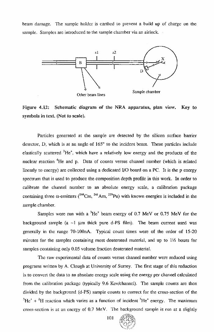
beam damage. The sample holder is earthed to prevent a build up of charge on the
sample. Samples are introduced to the sample chamber via an airlock. ·
sl s2
Other beam lines Sample chamber
Figure 4.12: Schematic diagram of the NRA apparatus, plan view. Key to
symbols in text. (Not to scale).
Particles generated at the sample are detected by the silicon srnface barrier
detector, D, which is at an angle of 165° to the incident beam. These particles include
elastically scattered 3He +, which have a relatively low energy and the products of the
nuclear reaction 4He and p. Data of counts versus channel number (which is related
linearly to energy) are collected using a dedicated 1/0 board on a PC. It is the p energy
spectrum that is used to produce the composition depth profile in this work. In order to
calibrate the channel number to an absolute energy scale, a calibration package
containing three a-emitters e44Cm, 241 Am, 239Pu) with known energies is included in the
sample chamber.
Samples were run with a 3He+ beam energy of 0.7 MeV or 0.75 MeV for the
background sample (a -1 ~m thick pure d-PS film). The beam current used was
generally in the range 70-100nA. Typical count times were of the order of 15-20
minutes for the samples containing most deuterated material, and up to 1 ~ hours for
samples containing only 0.05 volume fraction deuterated material.
The raw experimental data of counts versus channel number were reduced using
programs written by A. Clough at University of Surrey. The first stage of this reduction
is to conve11 the data to an absolute energy scale using the energy per channel calculated
from the calibration package (typically 9.6 Kev/channel). The sample counts are then
divided by the background (d-PS) sample counts to correct for the cross-section of the 3He+ + 2H reaction which varies as a function of incident 3He+ energy. The maximum
cross-section is at an energy of 0. 7 MeV. The background sample is run at a slightly
101

higher incident beam energy than the sample so that the front edge of the p energy
spectrum (corresponding to protons produced in reactions at the very surface of the
polymer film) lies at a slightly lower energy than the front edge for the sample of interest.
This reduces the risk of a slight mismatch in beam energies leading to a poor background
correction at the front edge.
Following the background correction the data are converted to counts versus
depth scale using the known stopping powers of 3He + in polystyrene and the theory of
elastic collisions. The counts are nonnalised to a composition scale by multiplying the
data by a nonnalisation constant such that the integral of the data over the sample
thickness matches the nominal volume fraction of the deuterated component in the film.
Statistical errors are calculated from the counts using Poisson statistics.
4.5 AUenuafed Tofal Reflec~iora (A TR) infraared specfroscopy
Samples for A TR spectroscopy were prepared by spin casting the polymer
solution directly onto the A TR crystal, which in this case was a silicon parallelepiped
(lOmm x 5mm x 50mm) with an angle 45°. No attempt was made to remove the native
silicon oxide layer that will be present on this substrate. The casting procedure was
virtually identical to that used to cast fihns for NR and NRA; a special adapter was
designed to facilitate the attachment of the A TR crystal to the chuck of the spin caster.
No problems were encountered, in terms of damage to the A TR crystal, for spinillng
speeds up to and above 4000 rpm. The shape of the A TR crystal - a narrow rectangle as
opposed to a disk - means that the film cast on the crystal is uneven in thickness towards
the ends of the crystal. For this reason the polymer fihn was removed from the frrst -1
em from each end (as well as from the entry and exit faces of the crystal) using an optical
tissue moistened with AR toluene.
All the A TR data presented in this work were obtained using a Perkin Elmer
1600 with a Specac variable angle A TR unit, which is illustrated in Figure 4.13.
102

Sample
ATRCrystal
Figu.n~re ~.B: Schematic illustration olf the §pecac VadalbRe A'f!R amnt, JPllarrn view.
lKey to symbols in text (Not to scale)
The infra red beam enters at the left and passes through the entry face of the A TR
crystal, where it undergoes multiple internal reflections. The stage on which the A TR
crystal is mounted can be rotated, however in this work it was fixed such that the
incident beam past through the entry face of the crystal normal to its surface. The
minors M 1 and M2 are used to couple the infra red beam leaving the A TR crystal to the
detector, which lies to the right of the region illustrated in the figure. The first step in
each measurement is to take an 'empty beam' spectrum without the ATR unit in the
optical path, this spectrum is used to coiTect data for absorption by atmospheric water
and carbon dioxide and for the variable energy output of the infra-red source across the
wavelength range. All spectra are automatically ratioed by this empty beam
measurement. The A TR unit is then placed in the optical path and the energy throughput
is maximised by adjusting the mirrors ml and m2. Before any measurements are made
on a polymer sample, the A TR spectra of the bare silicon crystal is obtained, this is done
so that the absorption of the silicon crystal can be accounted for. The spectrum of the
polymer film alone is obtained by subtracting the absorption spectrum of the bare silicon
from the spectrum of silicon crystal with polymer film.
The water and carbon dioxide absorption bands are not exactly subtracted,
because the concentration of water vapour and carbon dioxide varies as a function of
time (particularly if the experimenter breathes too close to the sample position!) and also
because the fine structure of the water band valies as a function of pressure and so the
bands will not subtract exactly if collected at different atmospheric pressures. These
effects contribute to the random enor found in Section 8.
103

All the spectra used in this work were the average of 64 scans (acquisition time -
5 minutes) and run at a resolution of 4.0cm-1• Some use was made of the intrinsic
spectrometer functions to give background subtracted spectra a flat baseline - this is a
cosmetic alteration. Absorption peak areas were calculated using the intrinsic peak area
function of the spectrometer. If necessary data can be obtained in the fonn of an ASCII
file of wavenumber versus absorption by converting the data to Lotus 1-2-3 format using
the Perkin Elmer 1720 spectrometer software and then reading the Lotus 1-2-3 data into
Microsoft Excel.
104

4J.6 /References tor Seciion 4J
1 . T. Kiff, unpublished results.
2. I. R. Peat, W. F. Reynolds, Tertrahedron Letters, 14, ]_1!)72, 1359.
3. R.K. Heenan, S.M. King, ISSI Conference, Dubna, September 1992.
4. G.D. Wignall, F.S. Bates, Journal of Applied Crystallography, 20, ]_1!)87, 28.
5 . J. Schelten, reported in reference 4
6. M. Rawiso, R. Duplessix, C.Picot, Macromolecules, 20, 1987, 630.
7 . T.P. Russell, Materials Science Reports, 5, 1990, 173.
8 . Neil Davidson, PhD Thesis, University of Strathclyde, 1984.
9. J. Brandrup, E.H. Immergut, 'Polymer Handbook 3rd ed. ', J. Wiley & Sons 1989, pp
V/82.
10. F.S. Bates, G.D. Wignall, Physical Review Letters, 57(12), 1986, 1429.
11 . A.R. Rennie, R.K. Heenan, ISSI Conference, Dubna, September 1992.
12. R.E. Ghosh, A.R. Rennie in 'Neutron Scattering Data Analysis 1990', ed. M.W.
Johnson, Institute of Physics Conference Proceedings.
13. A. Maconnachie, Polymer, 25, 1984, 1068.
14. FITFUN, R.E. Ghosh, Institut Laue Langevin, 1989.
15. W.H. Press, S.A. Teukolsky, W.T. Vetterling, B.P. Aannery, 'Numerical Recipes in
FORTRAN 2nd ed.', Cambridge University Press, 1992.
16. GENPLOT, Computer Graphics Service Ltd, Ithaca, New York, 1991.
17 . D. Meyerhofer, Journal of Applied Physics, 49(7), 1978, 3993.
18. J. Skilling in 'Maximum Entropy in Action' ed. B. Buck and V.A. Macaulay,
Oxford University Press, 1991.
105

This page left intentionally blank
106

The scattering data for blend I collected at temperatures 408K to 473K was
analysed using the RPA modified for polymers with a Schultz - Zimm distribution of
molecular weights. Fitting was carried out using the FORTRAN program Pullet3.
Fitting was carried out over the range 0.0 < Q < O.L.\-1, the Q range was limited because
deviations from the RP A expression were observed at higher Q values for all three blends
(B, D and I), these deviations will be discussed later. Three variables were allowed to
vary in the fitting process: x, Rgo and RgH. Values fitted for RgH varied over a wide
range, because the scattering was relatively insensitive to this parameter. Fits were
generally rather poor, see Figure 5.3, with consistent 1nis-fitting in the low Q region,
where the scattering is most sensitive to X·
N
0 * ,---....
0
0.04
0.03
'::::::' 0.02
0.01
~ ll [] c []
0.05 0.10
0/A
0 363K t::.. 383K + 408K X 435K
0.15 0.20
Figure 5.2: !Kratky plots of blend I cj> = 0.725 data as a function of temperature,
error bars from Poisson statistics.
111

I
E u
"' I
0.03
~ 0.02 .,.--..... a '---""
* "' a o.o1 + data -fit
0 . 0 0 LL..._L___L___i_i_i_i_i_i-1-L--L--L---'------'------'------'-----_l___J__~ 0.00 0.05 0.10 0.15 0.20
o;A-1
!Figure 5.3: Sample fit of the modified JRJ? A to the IO!emll X dlata, <j) = 0.478 at ~53K,
experimentaR error from Poisson statistics.
Figure 5.4 shows the variation of X with reciprocal temperature and composition. Error
bars are those calculated from the fitting procedure and do not include uncertainty
derived from errors in input parameters such as the degrees of polymerisation of the
blend components and their polydispersities. The X values for the blends at 473K are
rather more negative than the values obtained at lower temperatures. This may be
caused by sample degradation at higher temperatures, at the end of the experiment the
samples had turned brown and had a strong acrid odour. Aory - Huggins theory
suggests a X parameter which varies linearly with reciprocal temperature, for this reason
fits of the form shown in Equation 5.1 were made to the X data:
B x=A+
T
IEquatiorn 5.1
The parameters of these fits can be found in Table 5.3, the 473K data were excluded
from these fits.
112

Composition (<!>d-PMMA) A B
0.253 -0.016(3) 2(1)
0.478 0.010(5) -7(2)
0.725 0.002(2) -3(1)
l'abne 5.3: Parameters fntted to bBernd ! x data accordnrng to Equation s.:n.
l11ere is a fairly large variation of X with composition, in particular values for the <!> =
0.253 blend are rather more negative than for<!>= 0.478 and<!>= 0.725. Figure 5.1 shows
that the scattering from the <!> = 0.253 blend is considerably weaker than for the other
two compositions, one would expect that at higher Q values the scattering from the <!> =
0.253 and <!> = 0.725 would be similar, having corrected properly for background
scattering. This behaviour could be explained by an inappropriate transmission
correction arising from the presence of macroscopic air bubbles in the sample.
0.01
0.00
>< -0.01
-0.02 )(
0
0 )(
¢d-PMMA
0 408K D. 435K + 453K X 473K
-spinodal
Figure 5.4a: x vs <!>d-PMMA for biend ][, with Xs calculated from measured molecular
weights, error bars on 453K. data from fitting statistics
113

0.000
-0.005
>< -0.010
-0.015
-0.020
-0.025 0.0020
I
0
0.0021
0 0
0.0022 0.0023 T-1 /K-1
cpd-PMMA
0 0.253 6 0.478 + 0.725
0.0024
0
0.0025
Figure SAb: x vs ]_/T for !blend li, error bars on q, = 0.725 from fatting statnstncs
The average value for Rgn fitted for these data is 105±20A this compares with
68A calculated from literature1 values of <So/Mw12 > and the weight average molecular
weight.
Turning to the syndiotactic blends B and D, it is apparent from Figure 5.1 that
the scattering from blend B varies rather more with composition than for blend D. This
is because the deuterated polymer in blend B has a smaller radius of gyration and so
more of the scattering law is probed using the available Q range of LOQ. To use the low
Q limit of the Debye expression QRgn must be rather less than 1, using the literature
values to calculate the radii of gyration for the deuterated polymers the low Q limit for
blends B and D fall in the following regions:
Blend B
Blend D
Rgn z40A
RgD z 150A
0.0 < Q < 0.025k1
0.0 < Q < 0.0066k1
These values imply that the low Q limit may be used for the blend B data but for blend D
the low Q limit lies below the Q range available on the LOQ diffractometer.
Figure 5.5 shows data from blend B plotted in the Ornstein - Zernike mode (1-1 (Q) vs Q2)
suggested by the low Q limit of the Debye expression, the error bars are calculated from
Poisson statistics. The fluctuation correlation length ~ is calculated from the slopes and
114

intercepts of these plots and X is obtained from the intercept (given the value of Xs
calculated from the degrees of polymerisation of the blend components and the volume
fraction of the d-PMMA). In general the data are linear over the Q2 range 0.0002 < Q2
<O.OOOSA-2 but the data collected at 408K all show strong downward deviation from
linearity at low Q (this corresponds to excess scattering at low Q), for this reason data
collected at this temperature were fitted over the range 0.0004 < Q2 < 0.0008k2• lllis
downturn in the Ornstein - Zemike plot may be due to phase separation2 or the presence
of voids that are subsequently annealed out at the higher measurement temperatures. If
this is the case then X and ~ values calculated at this temperature may well be
meaningless. Data collected at 435K, 453K and 473K were fitted over the range 0.0002
< Q2 < 0.0008k2, the first few points, (below Q2 < 0.0002k2
) were not used because of
difficulty in subtracting the remnants of the straight through beam not masked by the
beam stop in this region. The straight line fit has been extended a little higher in Q2 than
the calculations of Rgn would seem to allow because the data remain linear in this slightly
extended region.
0.15
E u
"-...... 00.10
0 0.094 d-PMMA ~ 0.286 d-PMMA + 0.486 d-PMMA X 0.696 d-PMMA
0 . 00 ..__._,__,__..___..___..___..___..____,____,____,____.____.____.____.____.____.____.____.__.....____, 0.0000 0.0002 0.0004 0.0006 0.0008 0.0010
02/A_-2
Figure 5.5: Scattering from blend IB plotted in Ornstein- Zernike mode with linear
fits, errors from Poisson statistics (473K data)
115

Figure 5.6 shows X as a function of composition obtained from blend B, an
upturn in X is observed at low d-PMMA concentrations. Figure 5.7 shows X and ~-2 as a
function of reciprocal temperature (in K 1), extrapolating these plots to X = Xs and ~-2 =
0, respectively, for each composition gives the spinodal temperature, T,, at that
composition.
0.020
0.015
0.010
0.005 0
>< 0.000
A
+ +
-0.005 I
-0.010 .. -0.015
0.0 0.2
0
A
+
..
0.4 0.6
ci>d-PMMA
0 408K ~ 435K + 453K X 473K
-spinodal
0 ];
I
0.8 1.0
Figure 5.6: x vs «P data for bBend JB, with Xs caBculated error bars on 473K dlata
dlerived purely from fitting erron·.
116

0.020
0.015 <jld-PMMA 0
0 0.094 b. 0.286
0.010 + 0.486 X 0.696
0.005 A
>< 0 +
0.000 .. .. 6 0
lC ~ -0.005
0
-0.010 + A
-0.0~~0020 0.0021 0.0022 0.0023 0.0024 0.0025 T-1 /K-1
Figure 5.7a: X vs 1/T for blend B, error bars on cp = 0.486 from fitting statistics.
0.0025
0.0020 ~ I
<><( "--. 0.0015 ~ I oJ...J...I'
0.0010
0'008?oo2o 0.0021 0.0022 0.0023
T-1 /K-1
¢d-PMMA
0 0.094 A 0.286 + 0.48 X 0.696
0.0024 0.0025
Figure 5.7b: ~-2 vs 1/T for blend B, with straight line fits to 435K-473K data, error
bars on cp = 0.696 from fitting statistics.
117

For all four blend compositions the values of ~-2 at 408K are very similar and
deviate from the trends indicated by the values measured at 435K, 453K and 473K,
phase separation may be occurring in these blends and for this reason data collected at
408K has not been used in the spinodal temperature calculations. The data for blend B
with <1> = 0.094 are anomalous showing ~-2 increasing with increasing reciprocal
temperature, the data from the other three compositions show ~-2 decreasing with
increasing reciprocal temperature. The spinodal temperatures extracted in this manner
are shown in Table 5.4. The error bars shown are calculated from the fitting errors and
do not include contributions from other sources, most significant of which is the
unce1tainty in the detem1ination of the molecular weight of the deuterated polymer.
Assuming an uncertainty in this value of 10% a composition dependent systematic error
occurs in x. this error is -lxl0-3 for <1> = 0.094 and -2xl04 for the other compositions.
The calculated spinodal temperature is not affected by this error.
Within the experimental error the spinodal temperatures calculated from X and ~-2
are in agreement and show values of Ts that vary little over the composition range,
although it should be emphasised that the experimental error is large due to the limited
number of temperatures at which data were collected. Parameters to fits of the X data of
the fonn shown in Equation 5.1 can be found in Table 5.5.
Spinodal temperature (in K)
Blend Composition ( <l>d-PMMA) from X= Xs from~-2 = 0
B 0.094 370 ± 20 690 ±250
0.286 410 ±50 310 ± 60
0.486 420 ±20 370 ± 180
0.696 520 ±huge 360 ±huge
D 0.096 400 -
0.287 380 -
0.480 430 -
'fable SA: Spinodal temperatures calculated for ll>Rends lB and ]])
The blend B data were also analysed by fitting the full RPA expression using the
FORTRAN analysis program Pullet- the data were fitted over the Q range 0.0 < Q < 0.1
118

A-1, x. RgH and Rgo were allowed to vary. The fit was not extended over the full Q range
because the data clearly deviates from the RPA expression at high Q, this is observed for
both the blends B and D and will be discussed later.
Blend Composition (<!>d-PMMA) A B
B 0.094 -0.11(3) 49.3(5)
0.286 -0.13(4). 60(16)
0.486 -0.12(3) 53(12)
0.696 -0.03(3) 15(12)
D 0.096 0.40xl0-2 1.84
0.287 -0.20xl0·2 0.98
0.480 -0.32x10⁻² 1.86
'll'able 5.5: Values of A and! 13 JParameteu-s for tlhle aemJPeratu.nu-e dlependelllce of x
Values of X obtained were the same as those calculated using the Ornstein - Zernike
plots, within the experimental error. The average value of Rg0 fitted using this procedure
was 44±6A, which is consistent with the values calculated from literature values of
<So/Mw~ > and the measured molecular weight of the polymer which give radii of
gyration in the range 33A - 40A.
Moving on to the blend D data, the results from blend B and data in the literature
indicate that the low Q limit of the Debye expression is not probed by the LOQ
diffractometer for this blend. For this reason the data were only analysed by fitting the
RPA expression using the FORTRAN program Pullet. Fitting was over the Q range 0.0
< Q < O.lA-1 (the fitting range was limited for the reasons mentioned in relation to blends
I and B) and the parameters Rg0, Rgl-1 and X were allowed to vary. The average value of
Rg0 was 120 ± 50A which compares with values calculated from literature data of 130A
- 170A. Scattering was relatively insensitive to Rg1-1 and this was reflected in a huge
range of Rg1-1 values. Figure 5.8 shows typical fits obtained using this procedure, the
Kratky plot is used to emphasise the deviations from the RP A at higher Q values.
Figure 5.9 shows fitted values of X as a function of composition and reciprocal
temperature, in common with the data from blend B there is an upturn in X at low
volume fractions of d-PMMA. Uncertainty in the molecular weight of the deuterated
119

polymer leads to systematic errors approximately one order of magnitude smaller than
those for blend B. Within these errors the size -of the upturn in X at low d-PMMA
volume fractions is the same for both blend D and blend B. The variation of X with
reciprocal temperature is interesting, the X values measured at room temperature and at
408K are quite similar and coupled with the behaviour observed in blend B this would
indicate that phase separation was present in the samples at room temperature and that
this persisted at 408K but was absent in the blend at temperatures above 408K
0.04
IE 0.03
0 "-....
<'-1
9 0.02 ,----.... a '---/
0.01
0.481
0.287
0.096
% 30
d-PMMA
* % 30 d-PMMA
$ * = :E
d-PMMA
:E ! f
% :E I
% :E I
+data -fit
I I
I I
I I
0. 00 ..__..__..__.._.._.L_.L_.L_.L_.L_.L_.L_..L--'---'---'---'---'---'---'----'
0.00 0.05 0.10 o;.A.-1
0.15 0.20
Figure 5.8: Typical fits to lblemll D data (453K) olbtairned using PuiKet plotted in
Kratky mode, error bars from Poisson statistics.
120

0.0010
0.0005
+
+ 6 0
0 298K A 408K + 435K X 453K
-spinodal
0. 0 0 0 0 L___L____JL____JL--J---l---l--1---1.--L--'--L-L-___.__.__.__.___.___.__,____.
0.0 0.2 0.4 0.6 0.8 1.0
¢d-PMMA
!Fngure 5.9a: X vs <!> data for IIJHend IDl, wntln Xs cakllnlated from mo!ecu.nlar wenglilts,
error bars on .:a53K data from Poisson statistics.
0.0015 I I
cj> d-PMMA
0 0.096 A 0.287
0 + 0.481 0.0010 - 0 -
0 0
><
0.0005 r- -
<:> I I 6
~ 6
6
o.oo8?oo2o I I
0.0025 0.0030 0.0035 T-1 /K-1
Figure 5.9b: X vs 1/T data for lbDend IDl, error bars on <1> = 0.481 calculated using
Poisson statistics.
121

It is interesting to note that the errors purely from the fitting procedure are larger
for the data collected at room temperature and 408K than for data collected at 435K and
453K. Spinodal temperatures calculated from the X values measured at 435K and 453K
can be found in Table 5.4 and parameters of the fits to these data of the fonn shown in
Equation 5.1 are in Table 5.5. Clearly both these parameters and the spinodal
temperatures that have been calculated for this blend are somewhat tentative because
they are derived from data collected at only two temperatures.
122
5.li.3 Discussion
Two issues arise from the analysis of the scattering data from the isotactic blend
I: firstly the existence of crystallinity in the blends at 363K and 383K and secondly the
reliability of the X values extracted.
To recap the sample preparation and measurement procedure, which will have a
bearing on any crystallisation behaviour observed; powdered blends were held under two
tonnes of pressure at 373K for -1 hour and then allowed to cool for 1-2 hours before
being removed from the sample press, typically samples resided in the heated rack on the
LOQ diffractometer for periods of several hours at any particular measurement
temperature, pure h-PMMA and pure d-PMMA were run first at any particular
temperature and lower temperatures were run before higher temperatures. de Boeret aP have measured crystal growth rates, G, and melting points, Tm for hydrogenous isotactic
PMMA (Mv = 213,000) crystallised from the melt at a range of crystallisation
temperatures, Tc. For Tc = 373K de Boer et al observed a growth rate of -3A min-1,
producing crystals with melting temperatures of around 413K. This behaviour broadly
matches that observed in this work, the characteristic length scale of -215A calculated
from the position of the peak in the Kratky plots at low Q corresponds to crystal growth
times of -1 hour and the disappearance of the peak between 383K and 408K for the ~ =
0.725 blend and between 363K and 383K for the other two blends suggests melting
temperatures a little lower than those measured by de Boer, this lower melting
temperature could be due to the lower molecular weight of the isotactic d-PMMA -
work on polyethylene4 shows that Tm decreases with decreasing molecular weight
Crystallisation appears to be predominantly in the deuterated component. Given the
limited data collected from the crystalline samples in this work no further conclusions can
be drawn about the crystallisation behaviour of isotactic PMMA.
The validity of the X data extracted from the scattering from blend I relies on the
modified RPA that was used to analyse the data. The isotactic polymers used are clearly
highly polydisperse and the modified RPA was used in order to make some allowance for
this polydispersity but this modified RPA is based on a Schultz - Zimm distribution of
molecular weights. The reason that this distribution was used is that a simple analytical
expression for the scattering from this distribution is available, for general distributions
such a simple expression is not available. Figure 5.10 shows the actual distributions of
123

the isotactic polymers vs Log M measured usmg SEC and the Schultz - Zimm
distribution5 calculated from the polydispersity and molecular weight parameters derived
from the SEC.
0 measured -theoretical
0.004
en 0 ~ c 0.003 0 ~ 0
c 0
0 0 L 0 +-' 0.002
...0 0 L <( 0
0 0 00
0.001 0 OOOCXJ
0 CXJ
00 ooooooooco
0.000 1 03 104 105 106 107
Log1o M
Figm:e 5.10a: Mo!ecll.lllar wenght dlnstributnon for nsotactnc d-l?MMA, wnth
'tllleoretkan' §clunltz - Zimm dlistrnbution calculated using parameters from SEC.
en ........ c ~
0.003
c 0.002 0 L
+-'
...0 L <(
0.001
0
0
0 0
0 0
0 0
CXJ <XXXD
0 0
<D
0 0
0 0
0 0
0
CXJ CXJ 0
0 0 0
0
0 measured -theoretical
0
0 0
0
0
0
0
0
0 0
0
0 0
0
0 0
0
0 . 0 0 0 L----'---'-L.r-L-......._._._.______.__.__.....__._.L..L..L.Ju..____J._---L--'--'-...L...L...L.L.L.-----"'__,_--'--'~u.J
103 105
Log 10 M
Figure S.iOb: Molecular weight distribution for isotactic h-IPMMA, (see above)
124

The equation for the Schultz- Zimm distribution is:
w(M x) = PMx "-+I exp(-tM x)
where P is an arbitrary scaling constant and :
Mw h=--1
Mn
'A=l-h h
'A+l 't=--
Mn
lEqpuatnollll 5.2
lEquatnon 5.3
The shapes of the experimentally measured distributions and the 'theoretical'
distributions are quite different and for this reason the X values extracted using the
modified RPA are at best tentative. In addition there is some possibility that, even at
temperatures above 383K there is some crystallinity which even if not obvious could
effect the values of X calculated using the RP A, this may explain the rather poor fits to
the low Q region.
In summary: the results from the isotactic blend are tentative for two reasons: the
broad molecular weight distribution of the polymers and the presence of crystallinity. It
would be possible to fractionate broad molecular weight distribution isotactic PMMA to
give narrow molecular weight distributions, but the yield would be poor and this would
be particularly expensive for the deuterated polymer. Polymerisation at low temperature
to produce narrower molecular weight distributions is also possible but to produce high
molecular weight polymers reaction times are prohibitively long. Once narrow
distribution polymers have been obtained the crystallinity could be investigated using
SAXS or DSC. The X values measured for the isotactic blends will be discussed further
in the context of results from the syndiotactic blends and values for other hydrogenous I
deuterated blends found in the literature.
Isotopic blends of a single polymer have been used as simple model systems in a
number of studies, these include work on polystyrene6'7
, 1,4-polybutadiene2,
polydimethylsiloxane8, poly(ethylene-propylene)9 .to, poly(ethyl-ethylene)11
, poly(vinyl
125
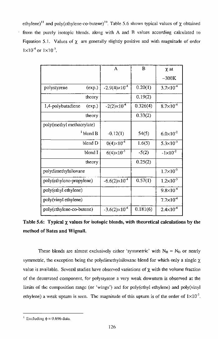
ethylene) 11 and poly(ethylene-co-butene) 10. Table 5.6 shows typical values of X obtained
- from the purely isotopic blends, along with A and B values according calculated to
Equation 5.1. Values of X are generally slightly positive and with magnitude of order
1x10⁴ or 1xl0-3.
A B X at
-300K
polystyrene (exp.) -2.9(4)x104 0.20(1) 3.7xl04
theory 0.19(2)
1,4-polybutadiene (exp.) -2(2)x104 0.326(4) 8.7xl04
theory 0.33(2)
poly(methyl methacrylate) 1 blend B -0.12(1) 54(5) 6.0x10⁻²
blend D 0(4)x104 1.6(5) 5.3xl0-3
blend I 6(4)xl0·3 -5(2) -lxl0-2
theory 0.25(2)
polydimethylsiloxane 1.7xl0-3
poly(ethylene-propylene) -6.6(2)xl04 0.57(1) 1.2xl0-3
poly( ethyl ethylene) 9.8xl04
poly(vinyl ethylene) 7.7xl04
poly( ethylene-co-butene) -3.6(2)x104 0.181(6) 2.4xl04
Table 5.6: Typical x values for isotopic blends, with theoretical calculations by the
method of Bates and Wignall.
These blends are almost exclusively either 'symmetric' with NH = N0 or nearly
symmetric, the exception being the polydimethylsiloxane blend for which only a single X
value is available. Several studies have observed variations of X with the volume fraction
of the deuterated component, for polystyrene a very weak downturn is observed at the
limits of the composition range (or 'wings') and for poly(ethyl ethylene) and poly(vinyl
ethylene) a weak upturn is seen. The magnitude of this upturn is of the order of 1x10·3•
1 Excluding <j> = 0.696 data.
126

These values for X and the magnitude of the upturn in the 'wings' of the composition are
in accordance with the values obtained for blend- D in this work, but the low molecular
weight blend B exhibits rather larger, more negative values for X than have previously
been observed in other isotopic blends. Although the size of the upturn in the 'wings' of
the composition range is similar to that seen in other isotopic blends. Both the A and B
parameters for blend B are far larger than are measured for any other isotopic blend.
The X value for blend I in Table 5.6 is negative because the temperature coefficient of X
is negative (unlike any other of the isotopic blends), at the measurement temperatures
values of X for blend I are broadly similar to those for blend B.
The range of X values measured exists in the context of a range of theoretical
work. Bates and Wignall12 have estimated X for isotopic polystyrene and polybutadiene
blends. They consider the mixing of two components as a two stage process, firstly
compressing or expanding each component to the segmental volume of the mixture and
then mixing the components at constant volume. Hence X is the sum of two terms, Xv,
from the volume change and xd from the mixing. It can be shown that:
Equation 5.4
where K is the compressibility of the polymers, VH, V0 and V are the segmental volumes
of the two components and of the mixture, k8 is the Boltzmann constant and T is the
temperature in K. Xd can further be divided into two, an enthalpic tenn Xdc and an
entropic tenn Xds:
Xd = Xdc - X,ts
lEquation 5.5
Xds is cannot be easily calculated but they state that it is small and positive and is
independent of temperature:
lEquation 5.6
127
aH and a0 are the segmental polarisabilities for the hydrogenous and deuterated
monomers and I is the segmental ionisation potential estimated from literature values 13•
Comparing these expressions with Equation 5.1:
A= -x,fs B = (Xv +xd£)T
lEqu.at8on 5. 7
Table 5.6 shows the values that Bates and Wignall calculate for the B parameter for
polystyrene and 1 ,4-polybutadiene along with a value calculated for poly(methyl
methacrylate). The calculated values for PMMA are very similar to those for polystyrene
and polybutadiene, these values being close to the experimentally measured values B for
the two polymers.
Freed and Bawendi14 have solved, exactly, the Amy-Huggins lattice model
(rather than using the mean field solutions) and they provide corrections for X as a
function of <1> and the degree of polymerisation of the blend components.
x= e(z-2) + Zc£2
+/ 2 _ 1 l+(_1 ___ 1_J2
(zc :4]-2 4 l N D + 1 N H + d N D N H zc
r 1 1 l 3zc£2
3e<J>lN + 1- N + 1J--2-<j>(l-<j>) D II
Equation 5.8
where £ is an effective interaction energy parameter and Zc is the lattice co-ordination
number, <1> is the volume fraction of the deuterated polymer. These calculations show
relatively large entropic corrections to X as the degree of polymetisation of one
component is reduced relative to the other, but the absolute size of this correction is far
smaller than that observed here. Similarly calculations using Equation 5.8 show upturns
in the 'wings' of the composition range, but again the absolute magnitude of these
variations is far smaller than those measured here.
Several models have been developed which are appropriate to describe these
simple isotopic blends, these include Monte Carlo lattice models15 •16
, polymer reference
interaction site models (PRISM) 17 and Flory-Huggins mean field theory, modified by
Muthukumar to allow for concentration fluctuations 18• (note equation 14 in reference 11,
128

based on this theory is incorrect19 as it is when repeated in relation to this work in
reference 20 ) generally thDugh the affect of asymmetry (No :f. NH) has not been
commented upon. Monte Carlo lattice models and PRISM do suggest a weak upturn in
X at the wings of the composition, but these upturns are typically small and indicate
downturns for negative X values. These calculations are all essentially aimed at
correcting or replacing the Flory-Huggins lattice stage of modelling.
Kumar16 has suggested that additionally contributions to effective X values arise
from failures of incompressible random phase approximation in particular non-ideal
volume changes on mixing. The size of the volume change required to produce the
observed upturn in X is very small (of the order of 0.05%). The data for blends B and D
are characteristic of 'repulsive' blends where there is a slight increase in the volume on
mixing, leading to upturns in X at the extremes of the composition range. Tang and
Freed21 have developed a compressible RPA theory, but its application to experimental
data is difficult.
In summary: for the 'high' molecular weight blend D the X values measured in
this work are very much in line with the X values measured for other isotopic systems,
both in magnitude and in the upturn in the 'wings' of the composition. The X values
measured for blend B, on the other hand, are negative and larger in magnitude than
values measured in any other isotopic blend. This striking difference in behaviour is
attributed to entropic contributions arising from chain length disparity. It is interesting to
note that the size of the upturn in blends B and D is very similar, this upturn is due
largely to failures in the incompressible RPA.
When using the RP A to extract X parameters from small angle neutron scattering
data the fitting range has been limited to lower Q values, this is because polymer chains
are known to deviate from the ideal; Gaussian distribution of chain segments upon which
the RPA is based. This behaviour has been known in PMMA for a long time, and has
been discussed by Yoon and Flory22• In addition to the non-Gaussian distribution of
chain segments, at higher Q values the 'rigid rod' nature of the chain at the level of the
monomer becomes apparent in the scattering. In order to further investigate this
behaviour the BIOSYM Polymer modelling software suite23 has been used to perfonn
Monte Carlo rotational isomeric state(RIS)24 theory calculations on PMMA chains.
Several model molecules were studied, in all cases the model molecule had 470 main
chain bonds and the scattering from 400 chain configurations was calculated at a
129

simulated temperature of 450K. Polymer molecules with 100% isotactic or 75%
syndiotactic dyads were used. For the 100% isotactic models only the backbone
scattering was calculated, but for the 75% syndiotactic blends the monomer units were
divided into scattering centres of the methylene groups on the main chain backbone, the
a methyl groups and the ester methyl groups. The total scattering from this molecule is
the sum of connibutions between scattering centres of the same type and cross tenns of
scattering from pairs of different types.
Figure 5.11a shows a comparison between the scattering calculated for a 100%
isotactic chain and the scattering from blend I, <P = 0.478 at 453K. In principle it should
be possible to scale the data by fixing 1(0) = 1 for both model and experiment, but the
excess scattering at low Q for the experimental data renders this impossible so the data
have been multiplied by an arbitrary scaling constant. The match is relatively good at
intermediate Q values. At low Q values the scattering is strongly influenced by the
molecular weight of the deuterated polymer and given that the molecular weight
distribution is broad the poor correspondence is unsurprising. Figure 5.11 b shows the
scattering from blend B, <j> = 0.486 at 453K, along with various scattering functions
calculated for a 75% syndiotactic chain, in this case it was possible to scale the model
successfully and experimental data by setting 1(0) = 1. The scattering from the ester
methyl groups appears to be dominant in the observed experimental scattering. These
model scattering profiles all show an upturn at Q values above -0.2A-1, this corresponds
to the scattering from a chain consisting of short 'rigid rods'. Unfortunately the available
Q range of LOQ does not extend far enough to test this behaviour in the experimental
system.
130

en +-'
c ::J
>-.0.0010 L
0 L
+-'
...0 L
<(
""-a o.ooo5
* N a
+ data -theoretical
0.05 0.10 0.15 Q/ ,&.-1
0.20 0.25
Figure 5.Ua: Comparison lbetweeHll scattering from bllend ][, <jl = OA/8 at 453K and
a JlUS calculation for the !backbone scaUernng from a ]_00% isotadnc cinann.
CIJ :t: c ::J
>-. 0.0010 L 0 L
+-'
...0 L <(
""-a o.ooo5
* N a
+ data -a methyl - -ester methyl -·-backbone methylene
-· -·-· .-·-
/ ~------------------
0.05 0.10 0.15 0.20 0/ ,&.-1
0.25
Figure 5.Hb: Comparison between scattering from blend B, <jl = 0.486 at 453K
and RH.S calculations from the scattering centres of the MMA monomer.
131

5. RA Conclusnons
l11e effective interaction parameter, x. of three d-PMMA/h-PMMA blends has
been measured. For the isotactic blend I the results are rather tentative because of the
large polydispersity of the polymers used, in addition clear signs of crystallinity were
observed at lower temperatures and at higher temperatures unusual scattering is
observed at low Q that may indicate the continued presence of crystallinity, possibly
invalidating the use of the RPA.
The values of X measured for blend D (an intermediate molecular weight d
PMMA blended with a high molecular weight h-PMMA) are comparable in magnitude to
values of X obtained for other isotopic blends. Blend B, where the molecular weight of
the d-PMMA is low, exhibits relatively large negative values of X and a much larger
temperature coefficient than has been observed for other isotopic blends. This behaviour
is attributed to entropic contributions arising from the strong asymmetry of the blend.
This conclusion is supported qualitatively by theory, although the magnitude of the
theoretical prediction is far smaller than the effect seen. Both blend B and blend D
exhibit an upturn in X at low volume fractions of d-PMMA. This upturn has the same
magnitude for both blends and is comparable to that observed in other isotopic blends.
The cause of such behaviour is not entirely clear, but it may well be a result of the failure
of the incompressible RPA caused by non-ideal volume changes on mixing.
Some RIS molecular modelling has been done to examine the deviation of the
observed scattering from that expected from polymers obeying Gaussian statistics.
These models show the importance of the substituent groups of PMMA in detennining
the observed scattering.
132

5.li.5 Refere111ces for Sect1o][] 5.li
1 . J. Brandrup, E.H. Immergut, 'Polymer Handbook 3rd ed.', (New York: John Wiley
& Sons, 1989), pp VII/36.
2. F.S. Bates, S.B. Dierker, G.D. Wignall, Macromolecules, 19, li986, 1938.
3 . A. de Boer, G.O.R Alberda van Ekstein, G. Challa, Polymer, 16, li976, 930.
4. C. Booth, C. Price, 'Comprehensive Polymer Science (val. 2)', (Oxford: Pergamon
Press, 1989) pp385.
5 . C. Booth, C. Price, 'Comprehensive Polymer Science (val. 1)', (Oxford: Pergamon
Press, 1989) pp294-296.
6. F.S. Bates, G.D. Wignall, Macromolecules, 19, 1986,932.
7 . D. Schwann, K. Hahn, J. Streib, T. Springer, Journal of Chemical Physics, 93(11),
1990, 8383.
8 . A. Lapp, C. Picot, H. Benoit, Macromolecules, 18, 1985, 2437.
9. M.D. Gehlsen, J.H. Rosedale, F.S. Bates, G.D. Wignall, L. Hansen, K. Almdal,
Physical Review Letters, 68(16), 1992, 2452.
10. W.W. Graessley, R. Krishnamoorti, N.P. Balsara, L.J. Fetters, D.J. Lohse, D.N.
Schulz, J.A. Sissano, Macromolecules, 26, 1993, 1137.
11 . F.S. Bates, M. Muthukumar, G.D. Wignall, L.J. Fetters, Journal of Chemical
Physics, 89(1), 1988, 535.
12. F.S. Bates, G.D. Wignall, Physical Review Letters, 57(12), 1986, 1429.
13. R.C. Weast, 'CRC Handbook of Chemistry and Physics 68th ed.', CRC Press, 1988.
14. M.G. Bawendi, K.F. Freed, Journal of Chemical Physics, 88(4), 1988, 2741.
15. A. Sariban, K. Binder, Macromolecules, 21, 1988, 711.
16. S.K. Kumar, Macromolecules, 27, 1994,260.
17. A. Yethiraj, K.S. Schweizer, Journal of Chemical Physics, 98(11), 1993, 9080.
18 . M. Muthukumar, Journal of Chemical Physics, 85(8), 1986, 4722.
19 . F.S. Bates, personal communication.
20 . I. Hopkinson, F.T. Kiff, R.W. Richards, S.M. King, H. Munro, Polymer, 35(8),
1994, 1722.
21 . H. Tang, K.F. Freed, Macromolecules, 24, 1991, 958.
22. D.Y. Yoon, P.J. Flory, Macromolecules, 9, 1976,299.
133

23 . Computational results obtained from Biosym Technologies (San Diego) Polymer
Module, version 5 .1.
24. P.R. Sundararajan, P.J. Flory, Journal of the American Chemical Society, 96(16),
ll974l, 5025.
134

5.2 Surface Enrichmenf
5.2.ll. ExJPernmeRlltaR
The aim of this set of experiments was to study the surface enrichment behaviour
of syndiotactic d-PMMA/h-PMMA blends as a function of the molecular weight of the
d-PMMA and the annealing time. To this end four blends were prepared, in each case
the h-PMMA 'matrix' had a molecular weight of 994,000 and the volume fraction of d
PMMA in the blend was ~0.17. This volume fraction of d-PMMA was chosen because
such a blend will have a nuclear scattering length density equal to that of the silicon
substrate, the intention was that this would make the presence of surface enrichment
more apparent in the reflectivity profiles. The molecular weight of the d-PMMA was
varied between 12,400 and 417,000. The exact volume fraction of d-PMMA in each
blend and the glass transition temperatures, T 8, of the five polymers used are shown in
Table 5. 7. Further details of the polymers used can be found in the section 4.1, the
'global' labels for the five polymers used are also given in Table 5.7. The blends will be
referred to in this section as blend A for the blend containing the lowest molecular
weight d-PMMA through to blend D containing the highest.
·' Mw <l>d-PMMA TJK
h-PMMA (TK21) 994,000 0 397.6
Blend A (TK24) 12,400 0.174 392.6
Blend B (TK25) 25,200 0.171 376.7
Blend C (TK26) 136,000 0.178 403.1
Blend D (TK23) 417,000 0.174 403.7
Table 5.7: ]J)etails of polymers and blendls
Thin films of each of these blends were spun cast onto silicon blocks from 5% w/w
toluene solution, the spinning speed was 4000 rpm. No attempt was made to remove the
native silicon oxide layer from the surface of the silicon. The thicknesses of the films
obtained were measured using contact profilometry, the variation in thickness over the
135
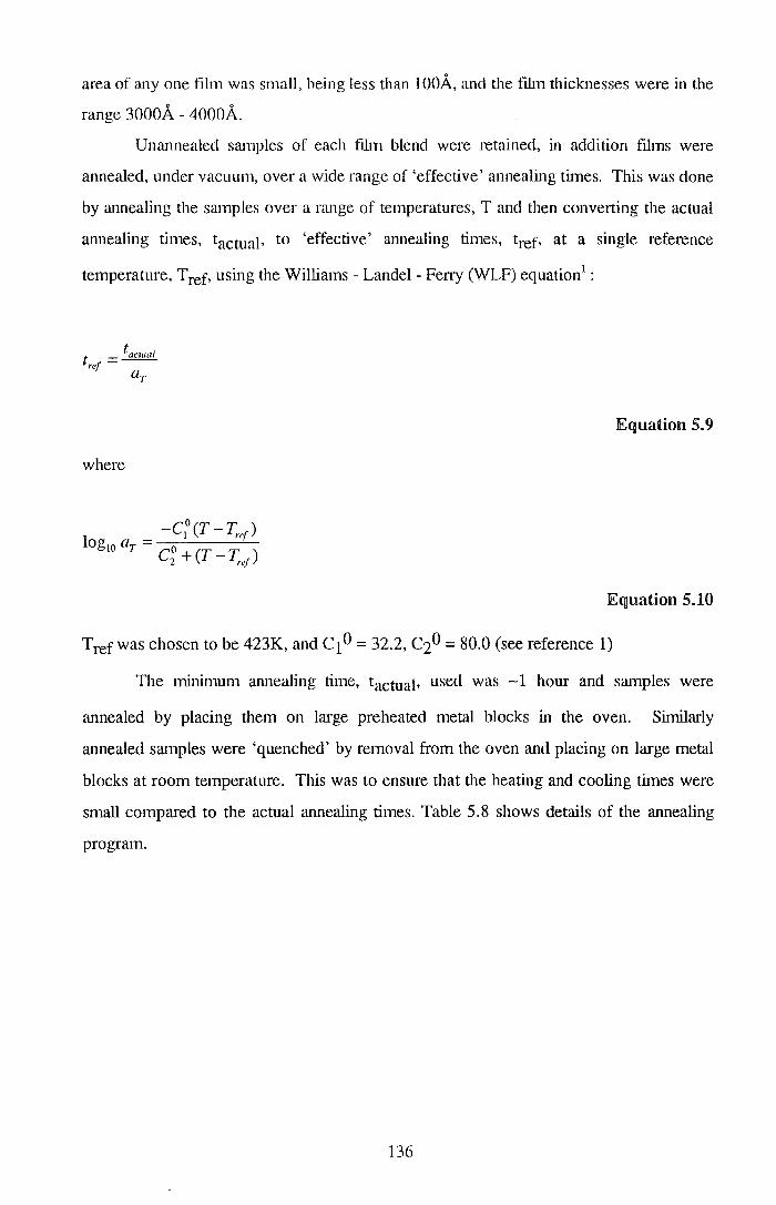
area of any one film was small, being less than IOOA, and the film thicknesses were in the
range 3000A - 4000A.
Unannealed samples of each film blend were retained, in addition films were
annealed, under vacuum, over a wide range of 'effective' annealing times. This was done
by annealing the samples over a range of temperatures, T and then convetting the actual
annealing times, tactual• to 'effective' annealing times, tref• at a single reference
temperature, Tref• using the Williams- Landel- Feny (WLF) equation1:
f _ f.zcwal ref-
ar
Equation 5.9
where
-clo (T - T,.,.,) log a = ·
10 T co + (T - T ) 2 ref
Equation 5.10
Tref was chosen to be 423K, and C1 0 = 32.2, C20 = 80.0 (see reference 1)
The minimum annealing time, tactual• used was -1 hour and samples were
annealed by placing them on large preheated metal blocks in the oven. Similarly
annealed samples were 'quenched' by removal from the oven and placing on large metal
blocks at room temperature. This was to ensure that the heating and cooling times were
small compared to the actual annealing times. Table 5.8 shows details of the annealing
program.
136

Actual Effective
Temperature/K Annealing time/min Annealing time/min Blends
411 1585 3.3x10⁻³ A,D
418 140 0.1 B,C
418 270 1.9 A,D
418 1390 9_9 A,D
418 1430 10 A,B
423 60 60 A,D
423 100 100 A,B,C,D
423 500 500 A,D
423 800 800 A
423 1000 1000 A,B,C,D
423 3000 3000 A,D
428 64 5000 A,D
428 102 8000 A,D
428 191 15000 A
428 255 20000 D
428 640 50000 D
428 1420 1.1x10⁵ B
433 270 l.Ox106 A,B,C,D
438 80 l.Oxl07 c 438 1030 1.3x10⁸ A,B,C,D
443 360 9.9x10⁸ c 448 207 9.6x10⁹ B,C,D
457 4230 1.7xl013 A,B,C,D
Table 5.8: Annealing program for d-PMMA/h-PMMA blends
137

5.2.2 Results
A representative selection of the reflectivity profiles obtained are shown in Figure
5.12, for clarity only the data from the unannealed samples are shown as points with
error bars, the number of points has also been reduced. The errors are calculated from
Poisson counting statistics. The reflectivity profiles were all very similar, they were all
smooth, all had very similar critical edges and only small differences were observed at
higher Q.
The reflectivity data were analysed in two ways: firstly the values for the
air/polymer intetface volume fraction of d-PMMA were calculated from the asymptote at
high Q of the RQ4 vs Q plot; this was done for all the data collected. Figure 5.13 shows
a typical RQ4 vs Q plot, the asymptote was calculated over the Q range 0.03-0.048A-1,
and over this range the data appears to have reached a constant value. The data in the
region 0.048-0.06A -1 were excluded due to the larger statistical error seen in this region.
Statistical error in the surface volume fraction calculated from such asymptote values
was in the range of 0.01-0.03. To evaluate the influence that surface roughness and the
silicon/polymer interface have on the values of surface volume fraction calculated in this
way, apparent smface volume fractions were calculated using the asymptote method
from simulated data derived from the optical matrix methods. Model profiles were
calculated for a series of volume fractions in the range 0.17-0.18 and the asymptotic
values were measured for these profiles using the same procedure that was used for the
experimental data. These measurements showed that there was a systematic over
estimation of the surface volume fraction of 0.014, but this over estimate was constant
over the range of bulk volume fractions used. This error probably arises from the Q
range used to calculate the asymptote being slightly too low, i.e. the RQ4 vs Q plot has
not yet reached its asymptote value, but increasing the Q range to higher Q leads to a
larger statistical error.
138

0
-2
(jl -4 0
__J
-6
0.02 0.03 0.04 0.05 0.06 o;.z.-1
lFngure 5.12a:Refledivnty pmfnles (lLogto(R) vs. Q) for !blend C Samples. (top)
unannealed sampUe, (middle) annealed for 3000 minutes effective tame and
(bottom) lxW13 minutes (effectnve time). 'fhe BaUer have been offset lby -1 and a2
units, for darity. lError bars are those arising from JPoisson counting statistics.
0
-1 ,-..... D:': ....__, ~ -2
(jl
0 _j
-3
-4
+ t=O min -t=3000 min - -t=1E13 min
0.02 0.03 0.04 0.05 0.06 o;.z.-1
Figure 5.121b: Reflectivity profiles (Log10(R) vs. Q) from blend D samples. Over
laid to show high degree of similarity !between data.
139

0.8
1 o.6 <X( '-...... '<t o ~ 0.4
0.2
0.02 0.03 0.04 o;'A-1
0.05 0.06
Figure S.B: JRQ4 vs. Q plot for blend! C sampHe, armeaHed for Jlxll013 minutes
(effective time) broken line shows value of asymptote, used! to calculate surface
volume fraction of d-.IP'MMA. JError bars show error arising from Poisson
statistics.
The effect of surface roughness is rather larger, increasing the surface roughness at the
air/polymer interface from OA to lOA causes the surface volume fraction obtained from
an RQ4 vs Q plot to fall below that used to simulate the data, a surface volume fraction
of 0.158 is obtained for a film with nominal bulk volume fraction of 0.187 and an air
surface roughness of lOA. The surface roughness of spun cast PMMA films was
measured using X-ray reflectivity and it was found that the air surface root mean square
roughness is around sA. The combined effect of the silicon/polymer intetface, surface
roughness effects and the slight over-estimate due to the Q range used on the measured
value of the smface volume fraction obtained from RQ4 vs Q plots is likely to be a slight
(<0.01) over estimate of the surface volume fraction. Figure 5.14 shows the values of
the surface volume fraction calculated using the asymptote method, values for the
unannealed films are shown at effective time = I0-4 minutes. Clearly for blends A, B and
C no enrichment of d-PMMA to the air surface is observed. It would seem possible that
a very small amount of smface enrichment is observed in blend D, using the asymptotic
method of calculating the surface volume fraction of the d-PMMA, but the 'enriched'
140

surface volume fraction observed is only slightly outside the error range derived from the
sources discussed.
Secondly a large subset of the data were analysed via optical mat.Iix methods
utilising a maximum enU'opy procedure2 to fit a free fonn model of 150 layers of fixed
thickness. Figme 5.15 shows examples of composition profiles obtained in this way, the
data have been offset by a factor of 0.1 for clarity. Figure 5.16 shows a selection of the
fits obtained using maximum enU'opy. Mis-fitting is almost exclusively in the critical
edge region. Figure 5.14 shows the values of the minimum and maximum volume
fraction of d-PMMA found in the top 250A, obtained from these free fonn fits. The
uncertainty in the minimum and maximum volume fraction d-PMMA in the top 250A,
arising purely from the Poisson counting statistics of the data, is in the range 0.005-0.01.
0.30 .----,,------.,----r,---.--,-----,,.------.,-----.
~ 0.25 r-2 Q_
I u 0.20 r- e
c 0
+-' 0.15 r-0 0 L
4-
Q) 0.10-E :::J
g 0.05-
. 0 0
a 0
0 a
0 a cif 0
" 0
Q a 0
. 0
0
0
"' a
0
o RQ~ vs. Q IJ MaxEnt
-
-
-
-
-
0. 00 L--__.1 ___ ..._ I _ __JI.__ _ ____~_I ___ L__I _ ____..LI __ --'
10-3 10° 103 106 109 1012 1015
Effective Time/min
Figure 5.14a:Air surface volume fraction for blend A. Open circles are data from
RQ4 vs. Q asymptotes. Closed squares are from maximum entropy fitted profiles
and indicate the range of volume fractions of d-PMMA found in the top 250A of
the profile. Data from unannealed samples is placed at Log( effective time)= -4.
141

0.30 I I I I I T
<( 0.25 1- -2
2 Q__
I 0.20 f- a -"D
c Q a 0 ~
0 v a a a a 0
a e e -+--' 0.15 1- e -u 0 8 a 0
a a 0
a
L 0 4-
<!) 0.10 ~ -
E 0 RQ4 vs. Q :J El MaxEnt -0 0.05 f- ->
0.00 I I I I I I
1 o-3 10° 103 106 109 1012 1015
Effective Time/min
Figure 5.14b: Air surface volume fractions of d-PMMA for blend B. For details
see Figure 5.14a above.
0.30 I I I I I I
<( 0.25 -2 -
2 0
Q__ • q
I 0.20 0
"D 1- -
a u II Q -c e " • .. " •
0 • " s B • -+--' 0.15 1- 0 • • 0 0 0 -u " 0 e
8
0 0 0
L 0 4-
<!) 0.10 1- -
E 0 RQ4 vs. Q :J II MaxEnt -0 0.05 1- ->
0.00 I I I I I I
1 o-3 10° 103 106 1 09 1012 1015
Effective Time/min
Figure 5.14c: Air surface volume fractions of d-PMMA for blend C. For details see
Figure 5.14a above.
142
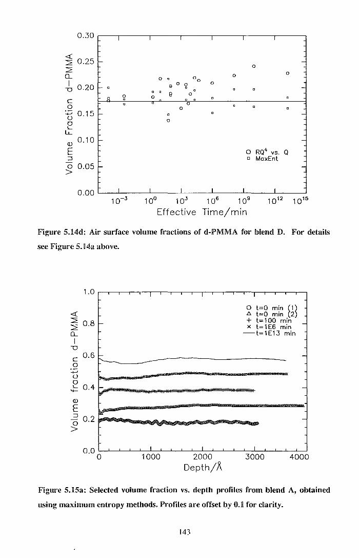
0.30
<( 0.25 2
2 D... I 0.20 -o
0 c 0
0
0
.......... 0.15 u 0 L.
LL
(1) 0.10
E :::J -0 0.05 >
0 0
0 0 g 0
0 0 g 0 0
0 0 0
0 0
0
00 0
0
0 0
0 0
0
0
0
0
0
0
0 0
0 RQ4 vs. Q o MaxEnt
1 0° 1 03 1 0 6 1 09
Effective Time/min
Figure 5 . .ll_4d: Air surface volume fractions of d.-IPMMA for !blend D. For details
see Figure 5 . .ll_4a above.
1.0 I
<( 2 0.8 2
r-
D... I
-o c 0.6 0
r-~
.......... u No. 0 L. 0.4 4--
r-l!f'"'
(1)
E :::J 0.2 -0
~ .-. ...... - ..... ->
0.0 I
0 1000
I
w.
-- -
I
2000 Depth/A
I
0 t=O min ~1 ~ t:. t=O min 2 + t=100 min x t=1E6 min -
-t=1E13 min
--
-
-~
I
3000 4000
Figure 5.15a: Selected volume fraction vs. depth profiles from blend A, obtained
using maximum entropy methods. Profiles are offset by 0.1 for clarity.
143
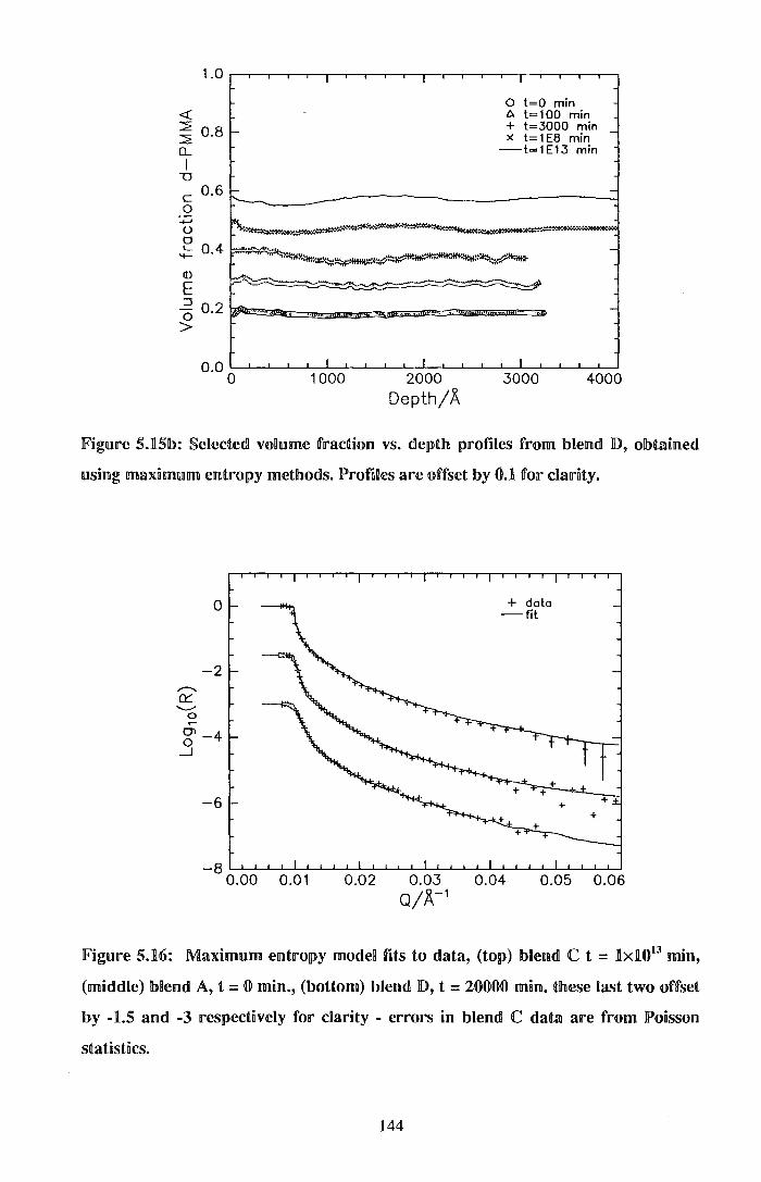
1.0
<{
~ 0.8 Q__
I -o c 0.6 0
+-' 0 a
.;: 0.4
Q)
E ::J 0 0.2 >
0.0
-
~~
~
be.~ ....
~
......
0
I
---
I
1000
I
I
2000
Depth/A
I
0 t=O min 1::. t=100 min + t=3000 min _ x t=1E8 min
-t=1E13 min
-
-Alt!s.
"""" "'"
- ..... ~
-
I
3000 4000
!Figure 5.:D.51b: §elected! voll"u.Bme 1fractio111 vs. dleiPth profn!es from lblHemll D, olbtanned
using maxim1Uim elllltropy metlllodls. l?rofnnes are offset by o.:n. Jfor cla~rnty.
+ data -fit
0.02 0.03 0.04 0.05 0.06 o;,&.-1
!Figure 5.16: Maximum entrOJPY model fits to data, (top) blellll(n C t = :D.x:D.013 min,
(middBe) lbBend A, t = 0 mnllll., (bottom) bBend D, t = 20000 mirn. tltnese last two offset
by -LS and! -3 ~respectnvely for clarity - errors in blend! C data are 1from l?onsson
statistics.
144
These maximum entropy fits appear to show weak concentration gradients in all the
films, even the unannealed films. The variation in the volume fraction profile between
the two different unannealed blend A films is as large as the variation between an
unannealed film and an annealed film. There are two explanations for this behaviour,
either these composition gradients really exist in the films and they arise during the spin
casting process or they are an artefact of the data analysis. If the gradients arose from
the spin casting it would be expected that during annealing the gradients in the bulk of
the sample would be removed. Free energy is required to maintain concentration
gradients and so the free energy of the system is reduced by removing the bulk
concentration gradients. Several of the composition profiles show very similar variations
in composition through the bulk of the specimen, characterised by a small amplitude, low
frequency spatial variation in volume fraction. A similar pattern appears in different
blends and for different annealing times which would suggest that it is an analysis artefact
rather than actual structure, such a low spatial frequency artefact could arise from a small
systematic mis-fitting near the region of total reflection. Model reflectivity profiles
incorporating absorption effects show that, even if the absorption term for h-PMMA is
1 Ox the predicted value, the effect of absorption is negligible. However if model
reflectivity data are generated using a range of 'simulated' resolutions (8-13%) and these
data are presented to the maximum entropy analysis program which in this case assumes
a fixed value for the experimental resolution of 7% then structures similar to those seen
in the fitted profiles are seen in the volume fraction profiles (see Figure 5.17). The
artefacts in the volume fraction profiles are thus explained by an experimental resolution
rather poorer than that calculated from the nominal slit geometry. This poorer resolution
could be due to alignment of the samples, sample quality (i.e. macroscopically uneven
samples) or slit setting. The most probable source of the reduced resolution is the slit
setting, the data presented here were collected before the new computer controlled slit
packages were installed on the CRISP beam line, the previous slit packages were
showing signs of physical deterioration. In conclusion, both asymptote and maximum
entropy analysis are in agreement and show no clear evidence for surface enrichment in
any of the blends over a wide range of annealing times and temperatures. This
conclusion is supported by SIMS work on blends A and D done by collaborators at the
University of Strathclyde.
145

<C 2 0.25 2 Q_
I -o 0.20
c 0 +' 0.15 0 0 L
4-
Q) 0.10 E ::J
g 0.05
+ t=1 E6 min -Simulation
0. 0 0 l___JL-JL..-JL.._j____L____.l____.L___J____L_...L.._...L..--L.-......L.-l...---'----'----'-....J...._....J.........J
0 1 000 2000 3000 4000
Depth/A
!Fngllllre 5.17: Volume fractUon vs. dleplth JProfille extracted! usang maximum enltropy
methods. 'fllne crosses are from reai data and! ltllne line is from simLillatedl data -
dlesigned to show !the effect of u.maccou.mtedl resohu.tion reductions.
146

5.2.3 Discussion
There are a number of possible explanations as to why no smface emichment was
observed in the d-PMMA/h-PMMA systems studied here:
(1) insufficient annealing time was allowed for the surface enriched layer to form.
(2) Flory-Huggins interaction parameter, x, is such that the blends are too distant from
the coexistence curve for enrichment to occur.
(3) there is insufficient surface energy difference between the d-PMMA and h-PMMA to
drive surface enrichment.
The WLF equation has been used by other workers3 '4 to increase the 'effective'
annealing time domain. Use of the WLF equation (i.e. annealing at different
temperatures) implies the belief that the polymer specimen under consideration is
effectively ideal i.e. there are no excess thennodynamic interactions. It was shown
earlier in this chapter (reference) that the interaction parameter, x, for h-PMMA/d
PMMA blends is not zero and varies with temperature, this will be discussed further
when item 2 is considered.
An altemative method of nonnalising the annealing data is by consideration of
self diffusion coefficient, Ds, of the low molecular weight component. Recently Liu et
a/5 published such data for blends of a series of d-PMMA molecular weights in a matrix
of h-PMMA (Mw = 980,000). These polymers were -40-50% syndiotactic and as such
had glass transition temperatures consistently lower than those of the polymers we used,
which are 70-80% syndiotactic. Liu eta/ find that:
D =kM -" s w
where k = 1.8x1o-6 cm2 s-1 g-1 mol
a=2.0
Equation 5.11
The data from which this expression was derived was collected at 418K, the temperature
dependence of the diffusion coefficient is described by an Anhenius type expression:
Equation S.U
147

where En is an activation energy, Van Alsten and Lustig6 have measured this to be 109
- kJ moi-l, combining these two expressions for the diffusion coefficient we find:
Equatnmn 5.B
where k' = 7.14xlo6 cm2 s-1 g-1 mol.
This expression allows us to estimate the diffusion coefficient for a probe d-PMMA in a
h-PMMA matrix with Mw "" 106 Mw over a range of temperatures and d-PMMA
molecular weights. In an attempt to allow for the effect of the differing tacticities of the
polymers used in Liu's work and in this work the diffusion coefficients will be calculated
using T g as a reference. Table 5. 9 shows variation of the diffusion coefficients, over the
range of temperatures used in the annealing program, estimated using Equation 5.13.
Diffusion coefficients/cm2s-1 Diffusion length range/ A
Blend 418K 433K 457K Low High
A 4.7xw-15 1.5x1Q-14 7.8xlo-14 520 14100
B l.lxlo-15 3.6x1Q-15 1.9x1Q-14 310 6940
c 3.9xw-17 1.2x1o-l6 6.5x1Q-16 60 1290
D 4.1xio-18 1.3x1Q-17 6.9xlo-17 15 420
Table 5.9: Diffusion coefficients and diffusion lengths
The quantity of interest when detennining how far towards equilibrium the
system has been annealed is the diffusion length (Dst)Y'l, where t is the actual annealing
time, these diffusion lengths are also included in Table 5.9. By this measure the range of
'effective' annealing times used is far smaller than the range calculated by the WLF
equation and shown in Table 5.8.
Jones and Kramer7 have studied the kinetics of enrichment for the d-PS/h-PS
system and they derive several approximate expressions for the rate of growth of the
smface excess z *, in particular the characteristic time, tc. of the approach to equilibrium
is given by:
148
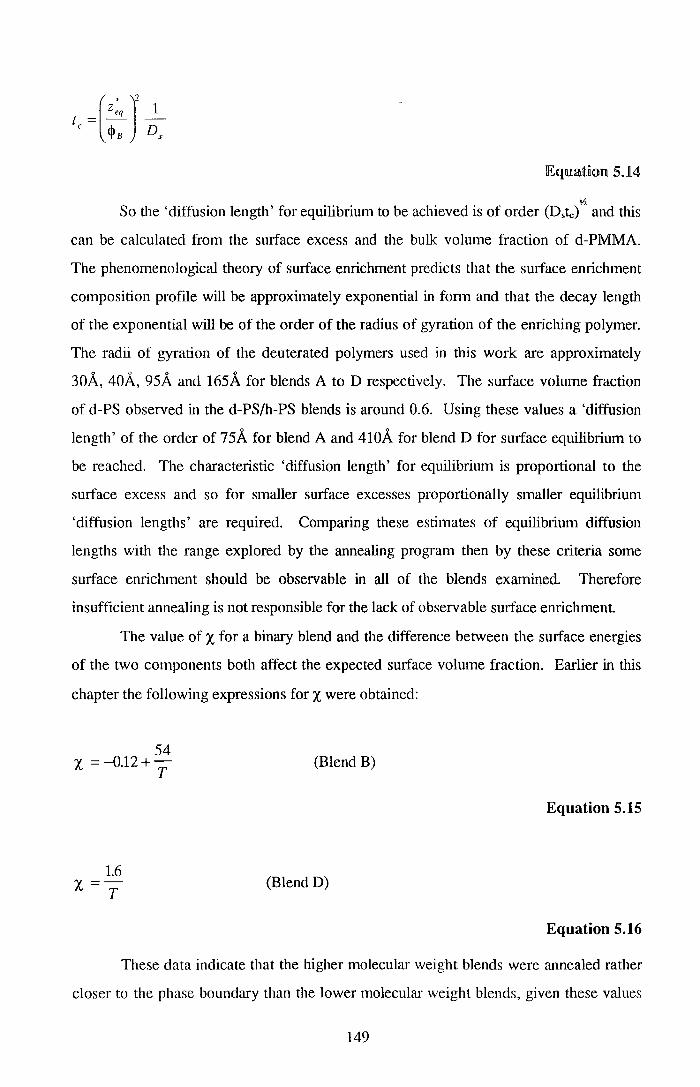
t =(z;q )2 _1 c IJls Ds
lEqltllatnmu 5.]_4
Yl So the 'diffusion length' for equilibrium to be achieved is of order (D,tc) and this
can be calculated from the surface excess and the bulk volume fraction of d-PMMA.
The phenomenological theory of surface enrichment predicts that the surface enrichment
composition profile will be approximately exponential in fonn and that the decay length
of the exponential will be of the order of the radius of gyration of the enriching polymer.
The radii of gyration of the deuterated polymers used in this work are approximately
30A, 40A, 95A and 165A for blends A to D respectively. The surface volume fraction
of d-PS observed in the d-PS/h-PS blends is around 0.6. Using these values a 'diffusion
length' of the order of 75A for blend A and 410A for blend D for surface equilibtium to
be reached. The characteristic 'diffusion length' for equilibrium is proportional to the
surface excess and so for smaller surface excesses proportionally smaller equilibrium
'diffusion lengths' are required. Comparing these estimates of equilibrium diffusion
lengths with the range explored by the annealing program then by these criteria some
surface emichment should be observable in all of the blends examined. Therefore
insufficient annealing is not responsible for the lack of observable surface enrichment.
The value of X for a binary blend and the difference between the surface energies
of the two components both affect the expected surface volume fraction. Earlier in this
chapter the following expressions for X were obtained:
54 X =-012+-. T
1.6 x=T
(Blend B)
Equation 5.15
(Blend D)
Equation 5.16
These data indicate that the higher molecular weight blends were annealed rather
closer to the phase boundary than the lower molecular weight blends, given these values
149

for X and assuming that the smface energy difference between h-PMMA and d-PMMA is
the same as that between d-PS and h-PS (i.e. 0.078mJ m-2) insignificant amounts of
enrichment for the low molecular weight blends (A and B) are expected but significant
amounts of enrichment for the highest molecular weight blend (D) and possibly blend
(C). Surface enrichment profiles for blend D, calculated using the expressions derived by
Jones and Kramer are shown in Figure 5.18, these expressions assume that the two
components of the blend have the same degree of polymerisation. The X parameters
used in Figure 5 .18a are the extremes of the range of values calculated for the annealing
program, this figure shows how the surface enriched layer becomes much thicker as the
coexistence curve is approached i.e. X increases. The differences in surface tension, used
in Figure 5.18b, range from the value found in the d-PS/h-PS system downwards. For
the systems modelled here the surface enrichment is virtually zero when the surface -2
energy difference is 0.02 mJ m . Entropic forces, favouring the low molecular weight
species at the surface, will enhance the surface enrichment slightly, this effect will be
largest for blend A an smallest for blend D.
150
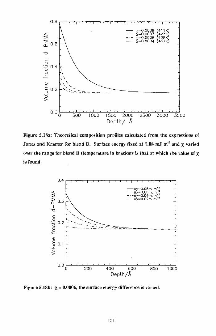
<( 2 2 Q_ 0.6 I
-o
c 0
Q)
~ 0.2
0 >
x=o.oooa !411 Kl x=o.ooo7 423K x=o.oooe 428K x=o.ooo4 457K
o.o 0 500 1 000 1500 2000 2500 3000 3500
Depth/ A
lFngure 5.].8a: Theoretical composition promes calculated from tlhle expressions of
Jones and Kramer for bRend D. Surface energy fixed at 0.08 mJ m·2 am! x varned
over the range for lbBend [) (temperature nn braclkets is that at whncll:n tll:ne value of x ns found.
<( 2 2 o_ 0.3 I
-o
c 0
-+-' 0.2 () 0 l-4-
Q)
~ 0.1 0 >
200
-~')'=0.08mJm - 2
- -~-y=0.06mJm-2
- · -~')'=0.04mJm-~ - · · ~')'=0.02mJm-
400 600 800 Depth/A
lFngure 5.].8b: X== 0.0006, the surface energy difference is variedl.
151
1000

Surface enrichment can be driven by surface energy differences too small to
measure directly. Experiments on the competitive adsorption8 of d-PS and h-PS from
solution onto Si02 show an isotope effect (with the d-PS adsorbing preferentially), in
contrast similar experiments9 using PMMA show no isotope effect. Granick attributes
this difference to the fact that PMMA interacts with the SiOz surface via the carbonyl
bond, which is not subject to the effects of deuterium isotope substitution. An attempt
was made to calculate the surface energy of d-PMMA relative to that of h-PMMA using
the parachor10• The parachor predicts surface energy by adding tenns from the atomic
composition and structural features such as double bonds and rings together. No data
are available for the contribution of the deuterium atom. The deuterium contribution was
estimated from the known difference in surface energy between h-PS and d-PS and then
this deuterium tenn was used to calculate the surface energy of d-PMMA, the surface
energy for h-PMMA was also calculated using the parachor. The difference between
these calculated surface energies is 0.06mJ m-2, about 75% of the difference between d
PS and h-PS. Clearly tl1is is a fairly crude calculation, but it does indicate that the
expected surface energy difference between d-PMMA and h-PMMA is rather less than
that between d-PS and h-PS. The neutron reflectivity data presented here suggest that
the surface energy difference between d-PMMA and h-PMMA is in the range 0.0 to
0.04mJ m-2.
Tasaki et a/11 have published neutron reflectivity data that indicate enrichment of
d-PMMA does occur in blends of d-PMMA and h-PMMA, where Mw (h-PMMA) z
330,000 and Mw (d-PMMA) varies from 12,000 to 330,000. The degree of enrichment
is very high (almost 100% d-PMMA at the surface), but the surface excess is very small
because the characteristic length of the enriched layer is very small (-lOA). The authors
make no mention of the background subtraction they have used and the reflectivity
profiles they show are characteristic of data from which no background has been
subtracted, the enrichment they observe may well be an artefact arising from incorrect
background subtraction. In addition the authors do not state the tacticity of their
polymers, but the annealing temperature used was 120°C, approximately 10°C below the
glass transition temperature of the polymers used here, but slightly above that of the
polymers used by Liu et al.
152

5.2A Conch.nsions
The surface enrichment behaviour of various low molecular weight probe d
PMMA in a high molecular weight matrix h-PMMA has been studied; over a range of
probe molecular weights and annealing times. Neutron reflectometry has been used to
determine the surface and near surface composition. No significant enrichment of either
the h-PMMA or the d-PMMA to the air interface has been observed, this is attributed to
an insufficient surface energy difference between the hydrogenous and deuterated
polymers. This is in contrast to the behaviour observed by other workers in the d-PS/h
PS system where deuteration does produce a large enough change in surface energy to
drive considerable amounts of d-PS to the air surface.
153

5.2.5 lRefereBllces for Section 5.2
1 . J.D. Ferry, 'Viscoelastic Properties of Polymers 3rd ed.', Wiley, 1980.
2. D. S. Sivia, W. A. Hamilton, G. S. Smith, Physica B, 173, li~~], 121.
3 . T.P. Russell, Material Science Reports, 5, ]_~90, 171.
4. G. Reiter, U. Steiner, Journal de Physique /I, 1, ].99:ll., 659.
5. Y. Liu, G. Reiter, K. Kunz, M. Stamm, Macromolecules, 26, ].993, 2134.
6. J. G. Van Alsten, S. R. Lustig, Macromolecules, 25, ].992, 5069.
7. R. A. L. Jones, E. J. Kramer, Philosophical Magazine B, 62(2), :ll.990, 129.
8 . P. Frantz, D. C. Leonhardt, S. Granick, Macromolecules, 24, ].99]., 1868.
9. H. E. Johnson, S. Granick, Macromolecules, 23, ].990, 3367.
10. D.W. Van Krevelen, 'Properties of Polymers 3rd edition', Elsevier, 1990.
11 . S. Tasaki, H. Yamaoka, F. Yoshida, Physica B, 180 & 181, 1~92, 480.
154

This page left intentionally blank
155
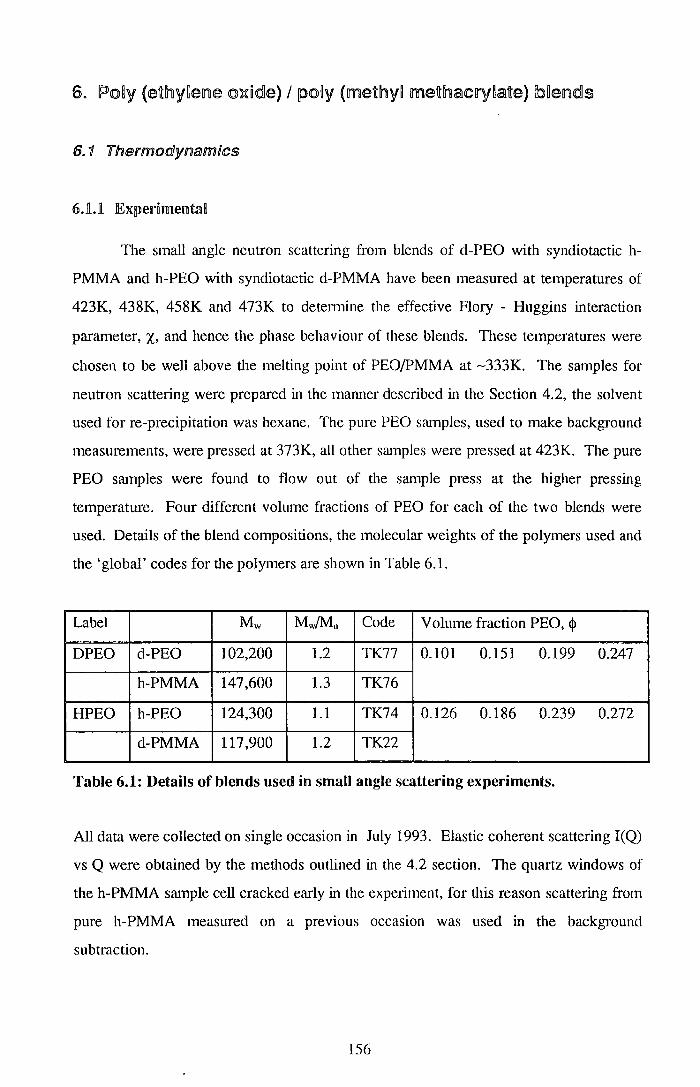
6. 1 Thermodynamics
6.:t1 lExpernmeJrntal
The small angle neutron scattering from blends of d-PEO with syndiotactic h
PMMA and h-PEO with syndiotactic d-PMMA have been measured at temperatures of
423K, 438K, 458K and 473K to detennine the effective Flory - Huggins interaction
parameter, x, and hence the phase behaviour of these blends. These temperatures were
chosen to be well above the melting point of PEO/PMMA at -333K. The samples for
neutron scattering were prepared in the manner described in the Section 4.2, the solvent
used for re-precipitation was hexane. The pure PEO samples, used to make background
measurements, were pressed at 373K, all other samples were pressed at 423K. The pure
PEO samples were found to flow out of the sample press at the higher pressing
temperature. Four different volume fractions of PEO for each of the two blends were
used. Details of the blend compositions, the molecular weights of the polymers used and
the 'global' codes for the polymers are shown in Table 6.1.
Label Mw Mw/Mn Code Volume fraction PEO, <1>
DPEO d-PEO 102,200 1.2 TK77 0.101 0.151 0.199 0.247
h-PMMA 147,600 1.3 TK76
HPEO h-PEO 124,300 1.1 TK74 0.126 0.186 0.239 0.272
d-PMMA 117,900 1.2 TK22
Table 6.1: Details of blends used in small angle scattering experiments.
All data were collected on single occasion in July 1993. Elastic coherent scattering I(Q)
vs Q were obtained by the methods outlined in the 4.2 section. The quartz windows of
the h-PMMA sample cell cracked early in the experiment, for this reason scattering from
pure h-PMMA measured on a previous occasion was used in the background
subtraction.
156

6.L2 !Resullts
Figure 6.1 shows examples of the elastic scattering, I(Q), for both the DPEO and
HPEO blends. At 423K the data show the trends in overall intensity that would be
expected for such blends, i.e. scattering increases as the volume fraction of PEO is
increased. The <1> = 0.126 HPEO blend exhibits much higher scattering at very low Q
values than the other HPEO blends, which show a downturn in this region. This is
probably caused by incorrect subtraction of the direct beam, at higher Q values the
relative intensities are as expected. There is generally no regular trend in the scattering
intensity for a single blend as a function of increasing temperature. Broadly the intensity
drops as the temperature increases, but the decrease between consecutive measurements
is not unifonn. For the <1> = 0.101 and <1> = 0.151 DPEO blends negative apparent
scattering is observed at high Q values for the higher measurement temperatures (458K
and 473K), clearly this is unphysical and must arise from the over subtraction of the
incoherent background. The <1> = 0.199 DPEO blend exhibits scattering considerably less
intense at 458K and 473K than at 423K and 438K, this may well indicate a less extreme
manifestation of the over subtraction of the background. The background scatter from
the blend is not necessarily the simple sum of the scatter from the pure components of
the blend, as has been commented upon in the section 4.2.4. Table 6.2 gives a broad
indication of the 'quality' of the I vs. Q data obtained, three categories have been used to
classify the data: ( ..1') the data conform with expectation in tenns of the shape of the I vs
Q profile and the overall intensity compared to the scattering of the same sample at
lower temperatures, ( x) the data exhibit negative apparent scattering in some parts of the
Q range. (?) the data do not exhibit negative apparent scattering, but the overall intensity
is low in comparison with scattering from the same sample at lower temperatures. It was
noted that air bubbles fanned in nearly all the samples during the course of the
experiment, an estimate of the degree of bubble fonnation at the end of the experiment is
shown in Table 6.3. The extent of the bubbles increased with increasing temperature.
The presence of air bubbles in the sample will have two consequences, firstly the flat
incoherent background will be over subtracted because more material will have been
accounted for in the background calculation than is 'seen' by the neutron beam, this
effect will be independent of Q. Secondly the intensity of the elastic coherent scattering
will be reduced, again because the amount of matetial 'seen' by the neutron beam is
157

reduced from the expected value; this will result in an observed elastic scatter that is
some fraction of the actual elastic scatter. The data will initially be analysed assuming -
only a correction in the incoherent background, subsequently an attempt will be made to
account for the expected scaling of the elastic scatter caused by the presence of air
bubbles.
Blend 423K 438K 458K 473K
DPEO (<j> = 0.101) ../ ../ j( j(
DPEO (<j> = 0.151) ../ ./ j( j(
DPEO (<j> = 0.199) ../ ../ ? ?
DPEO (<j> = 0.247) ../ ../ ./ ../
HPEO (<j> = 0.126) ../ ? ? ?
HPEO (<j> = 0.186) ../ ? ? ?
HPEO (<j> = 0.239) ./ ./ ? ?
HPEO (<!> = 0.272) ../ ? ? ?
'fabne 6.2: lEvahnatnon of tlhe quaHity of the I vs Q obtained for the bKends
Blend Rank Comments
DPEO (<!> = 0.101) 4 A number of large bubbles
DPEO (<j> = 0.151) 2 Several small bubbles near edges
DPEO (<j> = 0.199) 3 Several large bubbles
DPEO (<j> = 0.247) 1 No bubbles
HPEO (<!> = 0.126) 4 A number of large bubbles
HPEO (<!> = 0.186) 2 Several small bubbles near edges
HPEO (<j> = 0.239) 4 A number of large bubbles
HPEO (<j> = 0.272) 4 A number of large bubbles
'fable 6.3: IRanlknng of samples, as regards bubble formation, at ex.IJ1eriment end.
158

8
2
0.05 0.10 o;.A.-1
0 0.101 d-PEO b. 0. 151 d -PEO + 0.199 d-PEO X 0.247 d-PEO
0.15 0.20
Wiguure 6.1a: .IT(Q) vs Q for the [)JPEO lb!end at .:323K with ermrs fmm Ponsso~rn
statistics, as a function of composition.
30
.-I
E ~20 ,..-......
CY .....___.,
10
0.05 0.10 o;.A.-1
0 0.126 h-PEO 6. 0.186 h-PEO + 0.239 h-PEO X 0.272 h-PEO
0.15 0.20
Figure 6.1lb: I(Q) vs Q data for the HPJEO blend! at 423K, as a function of
composition
159

10
8
~
I 6 E 0
""'-,--...... CJ 4 '--"
2
0.05 0.10 o;A.-1
0 423K D. 438K + 458K X 473K
0.15 0.20
Figure 6.1c: I(Q) vs Q data for the DPEO blend cjl = 0.151, as a function of
temperature.
30
25
.-I E 20 0
""'-,--...... 1 5 CJ
'--"
10
5
0 423K D. 438K + 458K X 473K
Figure 6.ld: I(Q) vs Q data for the HPEO blend cjl = 0.239, as a function of
temperature.
160

Values in the literature1 for <SJMwv.,> indicate that the low Q limit of the Debye
function is not probed by the LOQ diffractometer for these blends. For this reason the
data were fitted using the FORTRAN program Pullet4, which fits the random phase
approximation allowing for the different volumes of the PEO and PMMA repeat units,
also included is a flat 'residual' background to allow for possible enors in the initial
background subtraction procedure. The data were fitted over the full Q range 0.008A-1
< Q < 0.21A-1• x, the 'residual' background and the radii of gyration of both blend
components were fitted. The X data obtained using these fits are shown in Figure 6.2.
There are quite large variations in X with temperature and composition, in the HPEO
blends these trends are fairly uniform, whereas for the DPEO blend there is a
discontinuity between values obtained for the samples at 423K and 438K (the 'good'
samples) and those obtained at 458K and 473K (the 'poor' samples). Representative fits
to the data are shown in Figure 6.3, in the fonn of Kratky plots. The fits to the data
were generally of a high quality and replicated the negative scattering at high Q observed
for some of the blends. The fit to the low Q region of the <P = 0.126 HPEO blends,
which exhibited unusual scattering at low Q compared to the other HPEO blends, was
rather poor. It was found to be impossible to fit the radii of gyration of both components
of the blends simultaneously, the scattering is not sensitive to both of these parameters
but rather the combination of the two.
Figure 6.4 shows values of the residual background fitted for the HPEO and
DPEO blends. The residual background fitted to the DPEO conelate well with the
evaluations of the data in Table 6.2, those samples deemed to be of the expected
intensity are fitted with a positive residual background and those with lower than
expected intensity are fitted with a negative residual background. The positive values
could indicate either that the incoherent background is initially under subtracted or the
residual background could be fitting deviations from the Debye function exhibited by the
scattering polymers. The HPEO blends were all fitted with negative values for the
residual background. The residual backgrounds fitted were up to 20% of the measured
incoherent background in magnitude, because the 'best' samples are fitted with positive
values and the worst with negative values of the residual background the incoherent
background subtracted could be as much as xl.4 the conect magnitude in the worst
case.
161

0.00
0 423K 6. 438K
-0.01 + 458K X 473K
0 A ~ A
A 0 + -0.02 0 =
+ >< :it
-0.03 +
:n:
-0.04
+ 1'{
-0.05 0.00 0.05 0.10 0.15 0.20 0.25 0.30
¢d-PEO
JFngUire 6.2a: x vs cjl for the IDPEO blend, fitted! using fixed Bllormalisation constant
and varying radii of gyration of the blend components.
0.00
0 42.3K 6. 438K
-0.01 + 458K I& 0
X 473K 0 A
0 + A
A +
-0.02
>< + X
+ -0.03
-0.04 X
- 0 . 0 5 '--L--'--'-''--'---'--.I........L-'-...l-''--'---'--.I........L--'-_.__'--'--'-..__.--'---'--.I........L--'--'--'--'
0.00 0.05 0.10 0.15 0.20 0.25 0.30
¢h-PEO
Figure 6.2b: X vs cjl for the HPEO blend, fitted using fixed normalisation constant
and varying radii of gyration of the blend components.
162

~
I
E 0.01 o u
N I
~ .,..--.. 0 .....__, * 0.005
N
0
0 423K 6. 438K + 458K X 473K
0. 00 0 b..£,L.......L-...JL-...JL-J~___j___j___j___j___j___j___j___j___j___j___j___jl-J..I--l...J
0.00 0.05 0.1 0 0.15 0.20 0/A- 1
Figure 6.3a: Representative fits to the DPEO data ($ = 0.151), using the Kratky
pRot Q2I{Q) vs Q. JDiata fatted using fixed rnormanisation cornstant and! varynng mdii
of gyration.
0. 0 2 0 .---.---.---.---.---.---.--.---.--.--.---.---.---.---.---.---.---.---.---.---.
~ 0.015 I
E u
N I ~ 0.010 ~
0 '---"
* N
0 0.005
0.000 0.00
0 423K 6. 438K + 458K x 473K
0.05 0.10 0/A- 1
0.15 0.20
Figure 6.3b: Representative fits to the HPEO data ($ = 0.186), using the Kratky
plot Q2I{Q) vs Q. Data fitted using fixed normalisation constant andl varying radii
of gyration.
163

0.3
0 423K -
0.2 ~ 438K A
+ 458K """0 X 473K 0
c + :::J " " 0 0.1 " L 0 {J) 0
0 ..Y u ~
0 0.0 ..0 +
0 + :::J -0.1 I """0 (/) lC
Q) L
-0.2
~
-0.3 0.00 0.05 0.10 0.15 0.20 0.25 0.30
¢d-PEO
Figure 6.4la: Values fntte<ll for the residual lbackgroun<ll to the Jl)JP'EO blend data,
normalisation constant fnxed, num of gyratimn of Uue !blend com!Poll1lents varied!.
0.3
0 423K
0.2 6. 438K + 458K
""D X 473K c :::J 0 0.1 L {J)
..Y u 0 0.0 _Q
0 .. 0 0 + " ::l -0.1
:i ""D + (/) + Q) L
-0.2 I
-0.3 0.00 0.05 0.10 0.15 0.20 0.25 0.30
¢h-PEO
Figure 6.4lb: Values fnttedl for the residual background to the JDl?EO blend data,
normalisation constant fixed, radii of gyration of the blend components varied.
164

This over subtraction of background should be associated with an equally large fractional
change in the coherent scatter, this would result in apparent X values that were
considerably more negative than the actual X values. To account for this reduction in the
coherent scattering the data were fitted using a varying value for the nonnalisation
constant. This was done using Pullet4, the values for the radii of gyration of the
components were fixed at the values calculated from the molecular weights of the
polymers and literature values for <SJM/'>. These were for the d-PEO = 98A, 108A
for the h-PEO, 86A for the d-PMMA and 104A for the h-PMMA. x, the residual
background and the nonnalisation constant were allowed to vary. Clearly the fitting of
the nonnalisation constant is somewhat undesirable and results obtained in this way
should be considered as tentative. The values of X fitted using this procedure are shown
in Figure 6.5. The tlu·ee parameters fitted were found to reach well defined values quite
rapidly. The quality of the fits was good, in fact the fit index's generated by Pullet4 were
identical for both methods of data analysis for any patticular sample, this would suggest
that the model profiles ru·e identical using these two fitting methods it is simply the
parameters used to generate the fit that are different. The expected value of the
nonnalisation constant for these data, in the absence of bubbles is 0.95, fitted values
ranged from very slightly above this value down to around 0.5 for some of the data
collected at 473K.
Comparing the values of x obtained using these two different methods of data
analysis, it was found that for the 'good' DPEO samples the fitted values of X are very
similar, see Table 6.4. Given this agreement for the 'best' satnples and the fact that the
analysis fitting the nonnalisation constant represents a solution to an expected
inadequacy in measured data the remaining analysis a11d discussion in this section will be
centred on the X values obtained using the method involving the fitting of the
normalisation constant.
There are several possible sources of error in the X values presented, excluding
the relatively small error that is indicated by the fitting procedure. Firstly there is the
possibility of a calibration error, this will effect both DPEO and HPEO blends equally
and so will not effect the conclusions drawn from the data. Secondly there is the
uncettainty arising from the values of the radii of gyration that have been calculated from
literature values of <SJMwv.,> and the moleculru· weights of the polymers. The
uncertainty in <SJMwy;,> is around 4% for PEO and 10% for PMMA. The uncettainty in
165

the molecular weights is around 10%, the square root of Mw is used in the calculation of
the radii of gyration and-so the error from this source is around 5%. Errors in <SJMw'h>
will effect both DPEO and HPEO blends equally, so relative differences in the X values
for these two sets of blends should be preserved, if this is the only source of error.
Uncertainties in the molecular weight may result in changes in the relative differences in
X between the DPEO and HPEO blends. In summary, the systematic error in the
absolute value of x, arising from uncertainties in <SJMw'h> and the calibration constant
are of the order of 10-15%. Relative statistical errors in X between the D PEO and
HPEO blends are of the order of 10%.
X X
(normalisation constant (nmmalisation constant
<J> (DPEO) T/K fixed) fitted) Difference
0.101 423 -0.0166 -0.0169 0.0003
0.151 423 -0.0195 -0.0181 -0.0014
0.199 423 -0.0185 -0.0181 -0.0004
0.247 423 -0.0162 -0.0188 -0.0026
0.101 438 -0.0182 -0.0178 -0.0004
0.151 438 -0.0173 -0.0182 0.0009
0.199 438 -0.0168 -0.0175 0.0007
0.247 438 -0.0160 -0.0178 0.0018
0.247 458 -0.0178 -0.0184 0.0006
0.247 473 -0.0200 -0.0200 0.0000
Table 6.4: Comparison of the 'good' DPEO data fitted using the two methods
presented in the text.
166

-0.005
-0.010
0 42.3K ~:> 4.38K + 458K X 47.3K
><-0.015
-0.020
-0.025
0 1:1.
+ I
- 0 . 0 3 0 L_.L.__.__L_.L.__.__L_.L.....L.....I--"=-....L.....I--'-...L.-L-'-...L.-L-'-...L.-L--'-.I..-1.--'--.I..-1.--'--"--l
0.00 0.05 0.10 0.15 0.20 0.25 0.30
¢d-PEO
JF'igure 6.5a: x vs cp for the Dl?EO !blend, fiUed using a varynng normanisation
constant and fixed radii of gyration for the blend components.
><
-0.020-! 0
+
-0.025-
0
0
0 0.101 d-PEO ~:> 0.151 d-PEO + 0.199 d-PEO X 0.247 d-PEO
-
-
I I I I I -O.OJ.8o21 0 0.00215 0.00220 0.00225 0.00230 0.00235 0.00240
Reciprocal temperature/K-1
Figure 6.5b: x vs ]_J'f for the DPEO blend, fitted using a varying normalisation
constant and fixed values for the radii of gyration for the blend components.
] 67
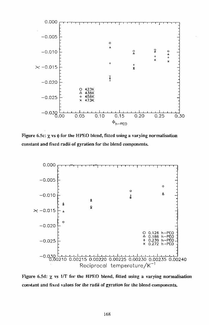
0.000
-0.005 0
6
-0.010 0 6
~ 0 6
+ + X
X + + >< -0.015 iK
-0.020 I
0 423K .6 438K
-0.025 + 458K X 473K
-o.o38.oo 0.05 0.10 0.15 0.20 0.25 0.30
¢h-PEO
Figure 6.5c: x vs cp for the lH!IPEO Tolendl, fnUed using a varying normalisation
constant and fixed radii of gyration for the blend components.
0.000
-0.005
-0.010
:!
>< -0.015 6
0
-0.020
-0.025
0
i
~
0
0 0.126 h-PEO .6 0.186 h-PEO + 0.239 h-PEO X 0.272 h-PEO
-0 038 . 0. 0210 0.00215 0.00220 0.00225 0.00230 0.00235 0.00240
Reciprocal temperature/K- 1
Figure 6.5d: x vs lt/T for the HPEO blend!, fitted using a varying normaBisatnon
constant and fixed values for the radii of gyration for the OJBend components.
168

<j>(PEO) A B/K-~- T.!K
DPEO 0.101 -0.12(4) 44(18) 360(190)
0.151 -0.034(4) 7(2) 190(60)
0.199 -0.04(2) 11(8) 240(240)
0.247 -0.03(1) 5(5) 150(150)
HPEO 0.126 -0.12(2) 47(8) 390(90)
0.186 -0.068(8) 25(4) 360(70)
0.239 -0.041(3) 14(1) 320(30)
0.272 -0.040(3) 13(1) 310(30)
'fable 6.5: A and lB parameters fnUed to the JDIPJEO and 11-HIPEO blend data
according to Equation 6.1
Table 6.5 shows parameters of fits of the form shown in Equation 6.1 along with the
spinodal temperature calculated from these fits.
B x=A+
T
Equation 6.1
A is the entropic contribution to X and B is the enthalpic contribution to X· The
reciprocal temperature dependence of the X values for the DPEO blends is non-linear,
this is reflected in the large errors in the fitted parameters. The variation in X with
composition is quite weak, except for the <!> = 0.101 blend where the X value measured at
473K is rather more negative than the values measured at lower temperatures. The
variation of X with reciprocal temperature for HPEO is rather more linear as is indicated
by the smaller values for the errors in the fitting parameters. There is a weak decrease in
X as <!> is decreased, again the <!> = 0.136 data are anomalous when compared to the data
at higher<!> values.
Although literature values of <SJMw~> indicate that the low Q limit of the Debye
function is not reached for these blends, when the data are plotted in the Ornstein -
Zemike mode (see Figure 6.6), they are found to be linear at low Q which is the
behaviour expected in the low Q limit of the Debye function. When linear fits to this
169

region are made and X values extracted from the intercept at Q = 0 the values of X
obtained are very similar to those obtained using the full random phase approximation.
There are larger deviations where negative values for the residual background have been
fitted using Pullet4, this is expected because this linear fit takes no account of errors in
the background subtraction.
E 1.0 0 ~
~ 0.5
0 0.101 d-PEO t::. 0.151 d-PEO + 0.199 d-PEO X 0.247 d-PEO
0.004 0.006 0.008 0.010 Q2 ;'A-2
Figure 6.6: Ornstein - Zernike plots for lDPEO blends at 423K, mustratnng the
linearity at low Q.
170

6.:t3 Discussnollll
The values of X detennined in this work can be compared to those which have
been obtained for other polymer blends. This discussion will concentrate on X values
determined using small angle neutron scattering, the systems for which X values have
been measured in this way can be divided into three categories:
(1) The very simplest 'homopolymer' blends, where a hydrogenous polymer is blended
with its deuterated counterpart, these systems have been discussed in this thesis in
relation to the h-PMMNd-PMMA blends.
(2) Systems where the two blend components are chemically very similar, such as
deuterated polystyrene (dPS) I poly (a. methylstyrene) (Pa.MS)2, poly (ethylene-co
propylene)(PEP) I poly (ethylene -co-butene-l)(PEB)3, polystyrene (PS) I Poly (bromo
styrene) (PBrSt § and blends of poly (ethylene-co-butene/ with various proportions of
ethylene and butene (dPEBx/dPEBy).
(3) Blends of chemically quite different polymers, these include deuterated polystyrene
(dPS) I poly (vinyl methyl ether) (PVME)5 •6
'7
, deuterated poly (methyl methacrylate)
(d-PMMA) I poly (styrene-co-acrylonitrile) (PSAN)8, deuterated polystyrene (dPS) I
poly (butadiene) (PB/, partially deuterated methoxylated poly (propylene glycol) (d 9 PPGM) I methoxylated poly (propylene glycol) (PEGM) , deuterated polystyrene (d-PS)
I poly (phenylmethylsiloxane) (PPMS)7, the interaction parameter for PEO/PMMA has
also been measured by Ito et a/10• Table 6.6 shows values of X obtained for systems in
these second two categories, in addition to small angle scattering measurements X has
also been measured for some of these blends using equation of state (PVT)
measurements (PEO/PMMAu, d-PSIPVME7, d-PS/PPMS7
) or by cloud point
measurements (PS/Pa.MS 12, PS/PVME12
). Values of the interaction parameter, from all
sources, for PEO/PMMA blends can be found in Table 6. 7
Examining the values of X in Table 6.6, it can be seen that the blends of
chemically similar components are characterised by a small ( -10-3) positive interaction
parameter. For the blends of more dissimilar components, d-PS/PVME has a relatively
large negative interaction parameter, this arises from specific interactions between the
styrene ring and the PVME13• Other systems (d-PS/PPMS, d-PS/PB, d-PPGM/PEGM),
§ Small Angle X-ray Scattering
171

exhibit equally large positive values of X suggesting unfavourable interactions between
the blend components.
X Temperature 1K Composition
d-PS/PaMS 0.005 503 0.5
PS/PBrS 0.003 403 0.5
DPEB!PEP 0.0013 353 0.5
dPEBx/hPEBy 0.001 440 0.5
d-PS/PVME5 -0.0368 298 0.5
d-PS/PVME6 -0.0359 298 0.5
d-PS/PVME7 -0.0598 298 0.31
d-PMMA/PSAN -0.0164 413 0.5
PEO/PMMA10 -0.0010 353 0.3
PEO/d-PMMA -0.004(6) 353 0.272
d-PS/PPMS 0.099 353 0.13
d-PSIPB 0.076 353 0.5
d-PPGM/PEGM 0.064 353 0.5
'fable 6.6: Values of x obtained for various blends using smaln angle scattering,
key to abbreviations and Hiteratuure sources in the text above.
Finally, there are the values of X from the d-PMMA/PSAN and PEO!PMMA blends,
these values are negative and not as large in magnitude as the values obtained for d
PS/PVME. These relatively small X values are probably the result of a combination of
favourable and unfavourable interactions, PMMA and PS are known to be incompatible
and are characterised by a positive interaction parameter14 of around 0.03. This
unfavourable interaction must be balanced and indeed exceeded by the dipole-dipole
interactions that would be expected to exist between PMMA and poly (acrylonitrile) in
the d-PMMA/PSAN system. Similarly it has been proposed that in the PEO/PMMA
system favourable interactions between the electronegative oxygen in PEO and the
electropositive carbonyl carbon in PMMA are opposed by repulsive forces between the
electronegative oxygens in both PEO and PMMA 15, leading to a weak overall
interaction.
172
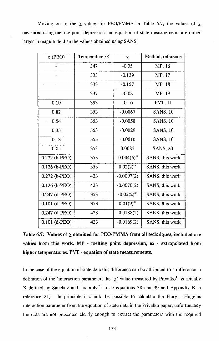
Moving on to the X values for PEO/PMMA in Table 6.7, the values of X
measured using melting point depression and equation of state measurements are rather
larger in magnitude than the values obtained using SANS.
<!> (PEO) Temperature /K X Method, reference
- 347 -0.35 MP, 16
- 333 -0.139 MP, 17
- 333 -0.157 MP, 18
- 337 -0.08 MP, 19
0.10 393 -0.16 PVT, 11
0.82 353 -0.0067 SANS, 10
0.54 353 -0.0058 SANS, 10
0.33 353 -0.0029 SANS, 10
0.18 353 -0.0010 SANS, 10
0.05 353 0.0083 SANS, 20
0.272 (h-PEO) 353 -0.004(6tx SANS, this work
0.126 (h-PEO) 353 0.02(2tx SANS, this work
0.272 (h-PEO) 423 -0.0097(2) SANS, this work
0.126 (h-PEO) 423 -0.0070(2) SANS, this work
0.247 (d-PEO) 353 -0.02(2tx SANS, this work
0.101 (d-PEO) 353 0.01(9tx SANS, this work
0.247 (d-PEO) 423 -0.0188(2) SANS, this work
0.101 (d-PEO) 423 -0.0169(2) SANS, this work
'fable 6.7: Values of X obtained for l?EO/PMMA from all techniques, included are
values from this work. MIP' - melting point depression, ex - extrapolated fmm
higher temperatures. IP'VT - equation of state measurements.
In the case of the equation of state data this difference can be attributed to a difference in
definition of the 'interaction parameter, the 'X' value measured by Privalko11 is actually
X defined by Sanchez and Lacombe21 • (see equations 38 and 39 and Appendix B in
reference 21). In principle it should be possible to calculate the Flory - Huggins
interaction parameter from the equation of state data in the Privalko paper, unfortunately
the data are not presented clearly enough to extract the parameters with the required
173

accuracy. Although melting point depression measurements give an indication of the
degree of polymer-polymer miscibility, through the medium of an interaction parameter,
there are both expelimental and theoretical difficulties22 which make the values of X
obtained somewhat inaccurate when compared to the absolute values measured using
small angle neutron scatteling.
Tuming to the other SANS data on the PEO/PMMA blends there are areas of
agreement and disagreement between this work and the work of Ito et a/10•
Extrapolating the values of X obtained in this work to the temperature at which Ito et a/
made their measurements (353K), it is found that the values of X obtained are the same,
within the substantial error which arises from the extrapolation. In addition the variation
in x over the composition range used here is the same as that measured by Ito. The only
difference this work and that of Ito is the measured temperature dependence of x; Ito et
a/ report that there is no temperature dependence in X over an 80K range for a <!>PEo =
0.54 blend, this is not in agreement with the behaviour observed here for blends with a
lower volume fraction of PEO. It is not clear from Ito et al which temperatures the 80K
range covers, but the implication is that Ito et al would expect values of X at 423K
considerably smaller than those measured here. There are a number of expelimental
differences between the work of Ito et at and this work, fiiStly the system being
measured is somewhat different, Ito et al studied blends of PEO/h-PMMA/d-PMMA,
varying the ratio of h-PMMA to d-PMMA in order to calculate the particle scattering
function, rather than assuming the Debye function used in t11is work. This approach
ignores any differences in X for h-PEO/d-PMMA and h-PEO/h-PMMA and assumes that
x for h-PMMA/d-PMMA is zero, other results in this work indicate that this second
assumption is invalid and work in this section strongly suggests that the first assumption
is also invalid. In discussing the influence of these effects on their measured X values Ito
et al do quote values for PEO/d-PMMA calculated using the apparent radius of gyration
for <l>h-PEo = 0.25, tl1ey find x = -9.5x10⁴, again this is within the error of the values
obtained here extrapolated to 353K, this suggests that the effect of deuteration on is
exceedingly small. Ito et a/ do not take account of the different segmental volumes of
PEO and PMMA in calculating x. re-calculating their values using the expelimental
values for the segment volumes leads to small conections, typically -0.0002.
The final observation to make of the work of Ito et al is the proximity of the
temperature at which measurements were made to the melting point of the blend;
174

measurements were made only 20K above melting point of these blends and were started
a relatively short time (20 minutes) after the measurement temperature was achieved, this
may mean that the samples had not reached equilibrium.
Deuteration is known to effect the phase behaviour of polymer mixtures, this is
shown in blends of hydrogenous polymers and their deuterated counterparts, the effect of
deuteration is to change X from zero (for a homopolymer) to -104. Graessley et aP
have studied the effect of swapping the locus of deuteration in blends of poly (ethylene
co-butene) with differing proportions of ethylene, this leads to changes in X of (2-S)xlo-
4, it should be noted that the polymers used by Graessley et aP were only partially
deuterated (30-50%). Russell23 has reported values of X for poly (styrene(S)-b-methyl
methacrylate(MMA)) block copolymers with either the styrene or the methyl
methacrylate or both partially deuterated (-50%), differences in x as large as 5x10·3
were observed between poly (d-S-b-MMA) and poly (d-S-b-d-MMA) and differences as
large as 9x10⁻³ when compared to values of x for poly (S-b-MMA) calculated from
cloud point curves14• Shifts in the cloud point of 30K between d-PS/PVME compared
with PS/PVME12, imply a change in X of -5xl0-3
, estimated using expressions for X as a
function of lj> and T that Han et af have calculated for d-PS/PVME, and simply
calculating the X values at 433K (the cloud point for h-PS/PVME) and 463K (the cloud
point for d-PS/PVME). This is a crude estimate that assumes that the change in X is due
entirely to changes in the entropic part of x. ( the parameter A in fits of the form of
Equation 6.1). Over the range of temperatures and conditions used in this work the
mean change in X between d-PEO/h-PMMA and h-PEO/d-PMMA blends was 8(2)x10-3,
this compares well with values from the poly (S-b-MMA) and PS/PVME systems.
Examining the values of A and B fitted to the X values according to Equation 6.1,
it can be seen that for the lowest volume fraction of PEO (either deuterated or
hydrogenous) A and B are rather larger than for higher volume fractions of PEO. This
behaviour arises from the downturn in X observed for the lowest volume fraction PEO
data, Kumar24 has pointed out that simply allowing for a non-ideal volume change on
mixing will lead to a downturn in X at the limits of the composition range. The
behaviour of this blend is characteristic of an attractive blend, i.e. where there is a
decrease in volume on mixing the components, the size of the effect observed is in
general agreement with the results in Kumar's paper. The relationship between X and the
175

'true' Flory- Huggins interaction parameter is given in Kumar's paper by Equation 6.2,
but attempts to replicate the effect quantitatively using this equation have failed:
!EqUiatnmn 6.2
(this is equation 29 from Kumar's paper). V o and V 11 are the partial volumes of the two -
components, N is the degree of polymerisation. p is the molar density. Equation 6.2
suggest that a plot of X versus 1/( <P (1 - <1>) should be linear and Figure 6. 7 shows that if
the data for the DPEO and HPEO blends are plotted in this manner there is indeed some
evidence for linearity (the symbols on this plot are the experimental data and the lines
least squares fits). It is interesting to note that the gradient of these lines changes from
positive to negative as the temperature increases. Clearly this analysis is rather tentative
given the limited <P range over which X values were measured. It is not clear why the
HPEO X data should be fitted relatively well using Equation 6.1 whilst the DPEO data
are fitted rather poorly, this could be due to the DPEO blend being further from a phase
boundary than the HPEO blend or a result of the air bubble formation that was observed
for these samples. For both blends the A and B parameters fitted to X for the blends with
the lowest volume fraction are the same, for the other compositions it appears that the A
parameters (the entropic part of X) approximately the same, but the B parameters (the
enthalpic part) are different, with the DPEO blend having significantly lower values forB
than the HPEO blend. The implication of this is that swapping the locus of deuteration
has changed the measured X values through the enthalpic contribution whilst the entropic
contribution remains unaltered, this result could be anticipated because simply reversing
the labelling in a blend should not change the entropy, but it is known that deuteration
changes the polarisability of the C-D bond (relative to the C-H bond) and this could lead
to changes in the enthalpic interactions, most probably via a change in the partial charge
of the ether oxygen in PEO.
176

-0.020 X ' " --'4-
' X ' ' >< ' ' ' -0.025 0 423K '
' t:. 438K ' ' + 458K ' ' X 473K
X
-0.030 4 6 8 10 12
1/¢(1-¢)
Figure 6./a: DPEO X data (symbols) plotted versus 1/ <j)(l - <j)), along with linear
fits (lines) to these data.
0
-0.010 ---tr"- b.
+ t...-. -·->< ........ X -·- ·-·-X ....... ·-·- ·-·-........ -·- +
........ + -0.015 0 423K .......
x·....._
!:> 438K ...... ........
........ + 458K ........
...... X 473K ......
·x
-0.020 4 5 6 7 8 9 10
1/¢(1-¢)
Figure 6.7b: HPEO data (symbols) plotted versus 1 I <j)(l- <j)), along with linear fits
(lines) to these data.
177

6.li.4l Conclusions
This work on d-PEO/h-PMMA and h-PEO/d-PMMA blends has emphasised the
need to exclude air from samples rigorously in order to detennine X with the minimum of
known parameters. In spite of the flaws in the expetimental procedure X values were
obtained, these values are negative and of intermediate magnitude, indicating that there
are weak attractive interactions in the blends, leading to 1niscibility over a wide
temperature range. Values of X for the DPEO blend lie in the range -0.017 to -0.029,
values for the HPEO blend lie in the range -0.007 to -0.019. These values are in
agreement with values measured by Ito et a/10, using small angle neutron scattering, for
PEO/PMMA. The change in X on switching the deuteration from PEO to PMMA is
8(2)x10-3 and is similar in magnitude to the change seen in other systems on changing the
locus of deuteration.
The variation of X with composition ts small except for the lowest PEO
concentration for which X is often significantly more negative than for the higher volume
fractions of PEO, this phenomenon can be attributed to non-ideal volume changes on
mixing. Fitting the X data for each blend and each composition with functions of the
form X = A + B/T, where A and B are entropic and entl1alpic contributions to X
respectively, it is found that the HPEO data are fitted well with functions of this form,
whereas the DPEO data are not. The values for the entropic part are broadly similar for
the two blends whilst the values fitted for the enthalpic part differ between the DPEO
and HPEO blends. This can be attributed to changes in the partial charges of ether
oxygen in the PEO, arising from the difference in polarisability between C-H and C-D
bonds.
178

6.1.5 !References for Section 6.1
1 . J. Brandrup, E.H. Immergut, 'Polymer Handbook 3rd ed.' (New York: John Wiley
& Sons, 1989), pp VII/36.
2 . A. Rameau, Y. Gallot, P. Marie, B. Farnoux, Polymer, 30, 1989, 386.
3. W.W. Graessley, R. Krishnamoorti, N.P. Balsara, L.J. Fetters, D.J. Lohse, D.N.
Schulz, J.A. Sissano, Macromolecules, 26, 1993, 1137.
4. T. Koch, G.R. Strobl, Journal of Polymer Science Part B: Polymer Physics, 28,
1990, 343.
5. M. Shibayama, H. Yang, R.S. Stein, C.C. Han, Macromolecules, 18, 1985,2179.
6. C.C. Han, B.J. Bauer, J.C. Clark, Y. Muroga, Y. Matsushita, M. Okada, Q. Tran
cong, I.C. Sanchez, Polymer, 29, 1988, 2002.
7 . S. Janssen, D. Schwahn, K. Mortensen, T. Springer, Macromolecules, 26, 1993,
5587.
8. K. Hahn, B.J. Schmitt, M. Kirschey, R.G. Kirste, H. Salie, S. Schmitt-Strecker,
Polymer, 33(24), 1992, 5150.
9. P.E. Tomlins, J.S. Higgins, Macromolecules, 21, 1988, 425.
10. H. Ito, T.P. Russell, G.D. Wignall, Macromolecules, 20, 1987, 2213.
11 . V.P. Privalko, K.D. Petrenko, Y.S. Lipatov, Polymer, 31, 1990, 1277.
12. J-L. Lin, R-J. Roe, Macromolecules, 20, 1987, 2168.
13. F. Ben Cheikh Larbi, S. Leloup, J.L. Halary, L. Monnerie, Polymer
Communications, 27, 1986, 23.
14. T.A. Callaghan, O.K. Paul, Macromolecules, 26, 1993,2439.
15. G.Ramana Rao, C. Castiglioni, M Gussoni, G. Zerbi, E. Martuscelli, Polymer, 26,
1985, 811.
16. E. Martuscelli, M. Pacella, W. P. Yue, Polymer, 25, 1984, 1097.
17 . M.M. Cortazar, M.E. Calahorra, G.M. Guzman, European Polymer Journal, 18,
1982, 165.
18. S.A. Liberman, A. deS. Gomes, E.M. Macchi, Journal of Polymer Science:
Polymer Chemistfy, 22, 1984, 2809.
19. P. H. Richardson, Ph. D. Thesis, Durham University, 1993.
20. J.M. Lefebvre, R.S. Porter, G.D. Wignall, reported in reference 10.
21 . I.C. Sanchez, R.H. Lacombe, Macromolecules, 11(6), 1978, 1145.
179

22. J. Runt, K.P. Gallagher, Polymer Communications, 32(6), lil!}l!}li, 180.
23. T.P. Russell, Macromolecules, 26, .lll!}93, 26.
24. S.K. Kumar, Macromolecules, 27, .ll.99~, 260.
180

6.2 Surface Enrichmenf
6.2.]_ lExjpernmellltal
The surface composition profiles of thin films of d-PEO/h-PMMA and h-PEO/d
PMMA were studied using neutron reflectometry and nuclear reaction analysis, where
the PMMA was syndiotactic. Table 6.8 shows the molecular weights and global codes
for these polymers, these are the same polymers that were used for the SANS work in
the previous section.
Mw Code
d-PEO 102,200 TK77
h-PMMA 147,600 TK76
h-PEO 124,300 TK74
d-PMMA 117,900 TK22
Table 6.8: Molecular weights and global codes for the poBymers used nn this
section.
The blends were each co-dissolved in chloroform and then spun cast onto silicon
substrates, the total weight percentage of polymer in the solutions was fixed at 2%. The
films were cast with a spinning speed of 4000rpm for 60 seconds, this produces films
around 2000A thick.
Three sets of experiments were done:
'NRA' experiments on two d-PEO/h-PMMA blends, containing different volume
fractions of d-PEO. These blends were annealed for a series of times at 423K. Details
of the bulk volume fractions of d-PEO in these blends, <!J8 , the annealing times, t, and the
labels used to designate these blends are shown in Table 6.9 (overleaf). PMMA is
sensitive to damage by the incident 3He + in the NRA experiment and for this reason the
samples were cooled with liquid nitrogen during the experiment. The NRA data were all
collected on a single occasion in March 1994.
181
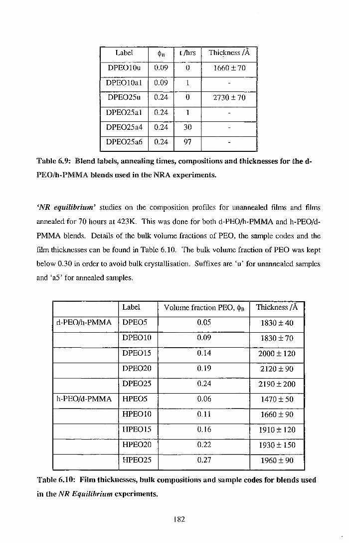
Label ~B t /Ius Thickness I A
DPE010u 0.09 0 1660 ± 70
DPE010a1 0.09 1 -
DPE025u 0.24 0 2730 ± 70
DPE025al 0.24 1 -
DPE025a4 0.24 30 -
DPE025a6 0.24 97 -
TabBe 6.9: IBlend Dall>els, anneaHing times, compositions and thicknesses for the da
PEO/h-PMMA blends used in the NRA experiments.
'NR equilibrium' studies on the composition profiles for unannealed films and films
annealed for 70 hours at 423K. Tlus was done for both d-PEO/h-PMMA and h-PEOid
PMMA blends. Details of the bulk volume fractions of PEO, the sample codes and the
film thicknesses can be found in Table 6.10. The bulk volume fraction of PEO was kept
below 0.30 in order to avoid bulk crystallisation. Suffixes are 'u' for unannealed samples
and 'a5' for annealed samples.
Label Volume fraction PEO, ~B Thickness I A
d-PEOih-PMMA DPE05 0.05 1830 ± 40
DPE010 0.09 1830 ± 70
DPE015 0.14 2000 ± 120
DPE020 0.19 2120 ± 90
DPE025 0.24 2190 ± 200
h-PEOid-PMMA HPE05 0.06 1470 ±50
HPE010 0.11 1660 ± 90
HPE015 0.16 1910 ± 120
HPE020 0.22 1930 ± 150
HPE025 0.27 1960 ± 90
Table 6.10: Film thicknesses, bulk compositions and sample codes for blends used
in the NR Equilibrium experiments.
182

These experiments were done on a single occasion in December 1992. The multidetector
was used and data were collected at incident angles of 0.25° and 0.6°, giving a Q range
of 0.005-0.06k'. Details of the experimental procedure can be found in Section 4.3.
(NR Kinetics' experiments were carried out to study the development of the
composition profiles with annealing time, t. This was done for d-PEO/h-PMMA blends
with bulk volume fractions d-PEO 0.19 and 0.23. Table 6.11 shows the annealing
program used. These blends will be referred to as DPE020 and DPE025 followed by
the suffixes shown in Table 6.11. Experiments were carried out on a single occasion in
March 1994, and the procedure was identical to that for the NR equilibrium studies.
Suffix Annealing time /hours
u 0
a1 1
a2 5
a3 16
a4 30
a5 70
a6 99
Table 6.11: Annealing program for the samples used in the NR Kinetics
experiments.
183
6.2.2 lResuUs
Before presenting the results of the NR and NRA experiments some brief
comments will be made on the thin film samples prepared for this work. The films of h
PMMNd-PMMA and h-PS/d-PS used elsewhere in the this work were very smooth; the
root mean square roughness over length scales of lOO's of microns was around 20A- as
measured by contact profilometry, X-ray reflectivity results show that over smaller
length scales the roughness is even less (- SA). The PEO/PMMA films prepared for tlus
work are far rougher, with root mean square roughness of between 50A and 170A. A
comparison of typical contact profilometry profiles of distance across sample versus
height are shown in Figure 6.8 for the annealed and unannealed DPE025 blends and an
annealed d-PS/h-PS blend. There is no reduction in the roughness of the DPE025 blend
on annealing the sample. It was noted that before annealing films of the DPE020 and
DPE025 blends exhibited an iridescent violet hue when viewed at a low angle. This
coloration was quite different to the colours normally seen in thin polymer films on
optically polished silicon substrates, which arise from interference effects. On annealing
the samples the iridescence disappears.
NRA
Figure 6.9 shows composition profiles derived from the NRA data for the
DPEOlO and DPE025 blends. These show a unifonn distribution of DPEO in both the
unannealed and annealed fiJms. The air-polymer interface is broader than that observed
in the polystyrene films, this is due to the larger roughness of these films. The apparent
thicknesses of the films are rather smaller than the values measured by contact
profilometry, tl1is is because the stopping distances for polystyrene were used in the
analysis of the data, instead of those for PEO/PMMA. It would be relatively
straightforward to re-analyse the data using the correct stopping distances but since this
would not effect the shape of the profiles this has not been done.
184

KA
04 1· •· : · · · · ·r ·1
0.21····· ··!··················· ················· .... , ....................... : ..... •'' ''' ·······!····J .. . . . . . .I
1: : : : : : ·:,
o o l!.i\.:.: .L ... : : . :.:.:...... . ... ·. : .... ··: :: . :: ····· ··!···· ·r ,. . . . . . ..
-o. 2 r' .·.'''' ''''.'.'.'' .. '' '.' .. ' '' ...... '.'.'.' ''' '' '.'.'' '' .. ' '.''' ''.'.' '.'' ... ' '''' - '.:' '.' j ;. . . . . . .I ,. . . . . ~ ..
-o. 4[' · · ·· · · 1 .................................................................................. : ~:J i· . · . . . .I
1 c,.. ............. : ...... ·····················r·d·o··········································zbri·························;···············Jb-o-······················ .. ijil) .. : ....... :.!l KA . ·Ill .
r·························T····················~·····································i···········~························.························=················································::,,
0.4r············:·······,;o/\···············:·············· ················•········ ···············r lj· . / : ', ~ ~ ~ -:,
- ~ . I . I . : . . u. z c............ . .. ·t .... ~ ... <.:.:.:1· ....... 'l' .... /:.:
1:.:.:.:1· ............. : .. ~ ....................... ··:,
1
.. I . I .. ······. . .. ·······1 Ill . .
: I : :,~· : I I 11 : .. ·:, : ••• I • I 'I . II I 11: II II ····. , ....
0 0 ,~··········1' . .11 .• ,1 .••.•... : .....•.... 1 ....... ,• ..... : .............. 1····1·· 1.1 '~ ~~· ~~ I ····~:. . :II I I I : I , .... .,.1, : I . ··:···· I;•. ···~~· ...... 1 ..... :1 : l I ..... : l,.o' : : I : 11 t I :
~~-~ (·) j ~ j ~ II ,I ~ \ / -~~ -o. 2 11 t ...... :' ........•........... ' ...... :.' ...• ' ... ' ..... ' .. ' .. :· ..... ' .•.. '.' .. ' .. '' ... :· ....... J '
-0.4 r'': .. ~::.1:: .I ~. :! .: :.······ .···········.······ ................. J KA 0 luu 200 ................................... 3(io}"""""'"""'• ..... ,JiO""""""··j
0 • 41::·:·:·:·. ,.,:::·:· .···:·:·:·:···:· :·. :·:·. :··.·:·.·.···:·:·.·.···:·:·.·.·:·:·:·:·:·.·:·:·.·.·.·.·:·:·.·:·.···········.·:·:·:·.:.·:·.···.·:·:·:·:·:·:·.·:·.·:·.·.···:·.· .I
0.21:·· .:···!·························· !······ ...... , ........................ : ..... /\·············j I;· lit, : ; ~··~ : ; ; II II .,,, . I • . I I • • • I I .
0. 0 j[··/ ... ~·~·~·:\1:.:.:·1.:-:·~\ ... j/ .. \,\. + ............ j. ·1:.- .............. )\ .. j. ·1:/· .... ·1,· ......... ·./l, :. ; 1, 11. I ; :
11 I 1,.1 11 11 : 11 ,.' ·
1
: . '·•. I • . I I •.,• I.. I I .; . . : : ·~.j.... 1 .. 1 ) ', II 1,!1 I I ., -0.2 r ..... .. ~· .............. ; ........... , .. \:.:.,/ ... , ... ! ..... '····"·:·:·:· ............ ; ............ \·· .. / ......
1
:
-o
4
/h 1. !6~ I. 2L . ;,)0 . "": il
1
IF'ngure 6.8: Plots of height versus horizontal displacement (from contact
pmfilometry) for (top) polystyrene, (middBe) ummnealed DPE025 and (!bottom)
DPE02Sa5- armeaDed 70 hoUirs. Vertical axes in kA, horizontal axes in J.Lm.
185

0.20
+ OPE010u t:,_ OPE010o1
0 w Q_ 0.15 I !1 6 """0 I 6!II± 66 6 c 6 I A 0 IIA H 6
+-' 0.10 0 I 0 II 66 I._
4-- :fAA (])
II E !6 :::l 0.05 ~A - A 0 > ~
~ ~
0.00 -500 0 500 1000 1500 2000
Depth /'A
Figure 6.9a: DPEOllO composition profiles obtained using nmdear reaction
analysis.
0 w 0.4 Q_
I """0
c 0.3 0
+-' 0 0 I._
4-- 0.2 (])
E ::J
0 0.1 >
+ OPE025u 0 OPE025a1 t:>. OPE025a6
0 500 1000
Depth /A 1500 2000
Figure 6.9b: DlPE025 composition profnles obtained using nudear reaction
analysis.
186

NR Equilibrium
Figure 6.10 shows sample reflectivity data for the DPEO and HPEO blends,
before annealing and after annealing at 423K for 70 hours. For the blends with volume
fractions of PEO 0.15, 0.20 and 0.25 there is an increase in the reflectivity on annealing,
this increase is largest for the DPE025 blend. These blends exhibit more off specular
scatter than the h-PS/d-PS and h-PMMA/d-PMMA blends, there is more off specular
scatter in the 0.6° data than in the 0.25° data. This off specular scatter is illustrated in
Figure 6.11, these are graphs of incident total neutron intensity versus position on the
multidetector. The data have been normalised such that the maximum of specular peak
has the same value and small shifts ( + 1 or +2) have been applied such that the specular
peak positions are identical, these are essentially cosmetic changes. As well as data from
d-PEO/h-PMMA Figure 6.11 includes data from a typical d-PS/h-PS sample which
exhibits virtually no off specular scatter, these data were all collected on a single
occasion. This implies that the behaviour observed for the DPEO blends is a property of
the blends rather than an artefact arising from, for example, inadequate shielding of the
straight through beam. The reflectivity data were analysed using two methods:
(1) Free fonn fits using the VOLFMEM program with a pixel size of 15A and
incorporating a 15A Si02 layer.
(2) Two layer fits using the PHOENIX program, also incorporating an Si02 layer.
A resolution of 6% was used in both these analysis methods, the reflectivity data is
essentially smooth and thus contains no information on the film thickness, for this reason
the film thickness was generally fixed at 2000A in the analysis programs except where
there was evidence for fringes arising from the film thickness.
Initially VOLFMEM fitted the annealed DPEO blend with an excess of d-PEO at
the air - polymer interface, this excess was quite large for the DPE025 blend and rather
small for the other blends, volume fraction profiles <j>(z) for this initial fit are shown in
Figure 6.12. However this excess of DPEO at the air- polymer interface is at odds with
SIMS data' collected from this system by collaborators at the University of Strathclyde
and XPS data2 for blends containing higher fractions of PEO, these workers both show
an excess of PMMA at the air-polymer interface.
187

0
-2
,---.... 0:: '---" 2-4
01 0
__j
-6
-8
OPE025
OPE01
0.00
:
... •.,
-Annealed 70 hours 0 Unannealed
0.02 0.04 0.06 0/A-1
Figure 6.10a: Neutron reflectivity data for selected DPEO blends. Symbols or
error bars - unannealed, lines annealed for 70 hours. DPE015 and DPEOS data
offset by D2 and -4 respectively for clarity.
-Annealed 70 hours 0 Unannealed
-8
0.00 0.02 0.04 0.06 o;'A-1
Figure 6.10b: Neutron reflectivity data for selected HPEO blends. Symbols or
error bars - unannealed, lines annealed for 70 hours. HPEO 15 and HPEOS data
offset by -2 and -4 respectively for clarity.
188

4x1 o-4
+ DPE020u 6 DPE025u
-DPE025a1
3 - -DPE020a6 - - Polystyrene
~ +-' (JJ
c 2 Q)
-l-' c .#-
+ .jtr+ t :.(-1~+
+-++- + +
~~ '!:# Mt>.
b-..~ ++ +
0 0 50 100 150 200 250
Position /mm
Figure 6.Ha: lPftot of intensity versus !POSition on muntidetector for a tyJPncaH
polystyrene blend and a selection of DPEO blends. Xncident angle ns 0.60°. Jl)ata
have been normalised to the same height at the specula&· peak.
0.000100 110 120 130 140 150 Position /mm
Figure 6.11b: Plot of intensity versus position on multidetector for a typical
polystyrene blend and DPE025u and DPE025a6. Incident angle is 0.25°. Data
have been normalised to the same height at the specular peak.
189

0.8
-DPE025a5 g~ 0
- -DPE025a5 - ·- DPE020a5 w -·· DPE010a5 " Q_ 0.6 I I
I I ~
-o I
c I 0
I +-' 0 0.4 I 0
I L 4-
I Q) I E
.....-....._ __ I
::l 0.2 / - '·,t.. ·-.-·-·-·-0 .,- . -·-·-·-.-·~·-· .- .. ---- \ > ___ .~,-- _.,/ .-·
\ I \ \ I
0.0 0 500 1000 1500 2000
Depth /A
Figure 6 . .ll.2: Composition versus depth profiRes for selected a11meaHed JDJPIEO
lbDends, obtained using VOLFMIEMI. For the JI)PJE025 blend! models witlhl am excess
of dl-PEO at the CR.) air or (2) substrate interface are obtained.
In addition it has already been observed that the surfaces of these blends are very rough
and the effect of this will be to reduce the apparent volume fraction of d-PEO at the air
polymer interface fitted by the program VOLFMEM, which does not explicitly include
the effects of surface roughness. Retuming to the data it was found that another model
could be fitted to the annealed DPE025 data using VOLFMEM, in this case there is a
depletion of d-PEO from the air-polymer interface (corresponding to surface roughness
and possibly an enrichment of PMMA) and an excess of d-PEO at the Si02-polymer
inte1face. This profile is also illustrated in Figure 6.12. The nonnalised X2 parameters
for these fits are 0.8 and 3.0 for d-PEO excesses at the air-polymer and Si02-polymer
interfaces respectively. The fits of these two models to the reflectivity data are shown in
Figure 6.13. The model with an excess of d-PEO at the air-polymer interface gives the
better fit, although the model with the d-PEO excess at the Si02-polymer interface also
gives a very good fit. However given the XPS and SIMS data and the likely effect of a
large surface roughness it is probable that the model with a d-PEO excess at the Si02-
polymer interface is the correct physical desc1iption. Attempts were made to encourage
VOLFMEM to fit similar compositions to the other <mnealed DPEO data, but these
190

proved unsuccessful. However two layer models, with an excess of d-PEO at the SiOr
polymer interface and a large- air-polymer interfacial roughness, were fitted to all the
annealed DPEO data using PHOENIX.
······data - · · Excess at air (VOLFMEM) - · -Excess at substrate (VOLFMEM) - -Excess at substrate (two layer model)
0.02 0.03 0.04 0.05 0/A- 1
0.06 0.07
Figure 6.13: Neutron reflectivity data for DPE025a5, with fits using VOLFMEM
models with d-PEO excesses at the air or substrate interface and a two layer model
with daPEO at the substrate interface.
The parameters of these fits ru~e shown in Table 6.12, where Zt~> <l>n and crn are the
thickness, volume fraction d-PEO and roughness of the nth layer, the air-polymer
interfacial roughness is cr0 • Also included in Table 6.12 is the fit index, which is not
identical to the nonnalised X2 parameter more commonly used to indicate fit quality.
Tables of the correspondence between fit index and nonnalised X2 parameter can be
found in Section 7.2 (Table 7.7) and Section 8.2 (Table 8.3). Briefly fit indices of 0.06,
0.12 and 0.16 correspond to nonnalised X2 parameters of 4, 8 and 19 respectively. The
smface excesses at the polymer - Si02 intetface z*s; = z2*C<I>r <!>I), are also shown in
Table 6.12.
191

Go/A <!>I Zj ;A crdA <1>2 Z2/ A Fit Index excess,-z*sJA
DPE05a5 429 0.05 1870 55 0.42 41 0.18 15
DPE010a5 660 0.10 1700 78 0.41 61 0.12 19
DPE015a5 641 0.15 2000 108 0.48 80 0.13 27
DPE020a5 336 0.16 2000 88 0.51 82 0.13 29
DPE025a5 674 0.24 2000 56 0.72 95 0.06 46
Table 6.12: Fit parameters for two layer PHOENIX fits to the annealed DPEO
blend data.
Figure 6.14 shows a selection of the composition profiles shown obtained using these
parameters. The polymer- Si02 interface is at the left of this graph.
0 w 0.8 Q_
I -o
c 0
-+-' u 0 L
4-
Q)
E ::::::1
-0 >
0.6
0.4
0.2
0.0
-DPE025a5 - -DPE015a5 -· -DPE05a5
' -------------'
0 100 200 300 400 500 Depth (from Si)/A
Figure 6.14: Selected composition vs depth profiles for the annealed DPEO blends,
obtained using two layer model fits with roughness. Horizontal axis has substrate
interface on the left.
The air-polymer inteifacial roughness fitted to these data is very large, larger even than
the value obtained from the contact profilometry data, but the reflectivity profile is
192
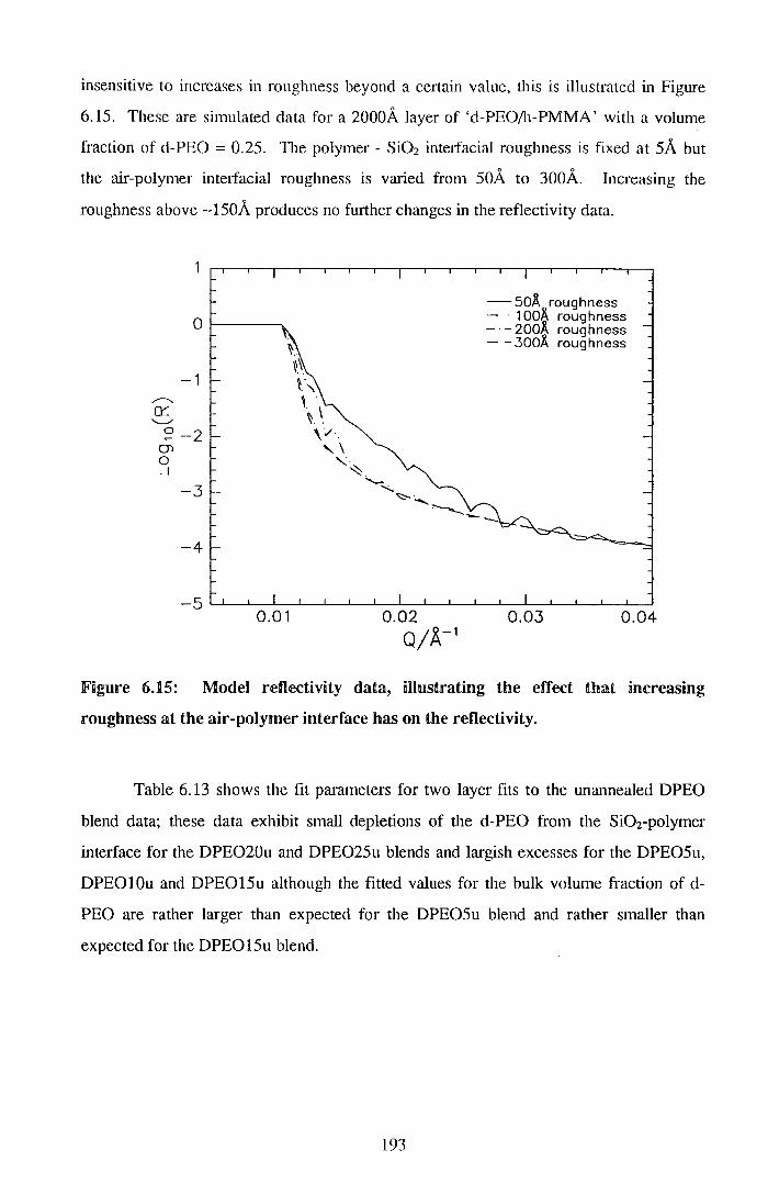
insensitive to increases in roughness beyond a certain value, this is illustrated in Figure
6.15. These -are simulated data for a 2000A layer of 'd-PEO/h-PMMA' with a volume
fraction of d-PEO = 0.25. The polymer - Si02 interfacial roughness is fixed at sA but
the air-polymer intetfacial roughness is varied from soA to 300A. Increasing the
roughness above -150A produces no further changes in the reflectivity data.
01------,.
-1 ,-----... 0:::: '----" 2-2
Ol 0 _J
-3
-4
0.01 0.02 o;,&.-1
-so.&. roughness - .. 1 oo.&. roughness - ·- 200.&. roughness - -300.&. roughness
0.03 0.04
Figure 6.15: Model reflectivity data, illustrating the effect that increasing
roughness at the air-polymer interface has on the reflectivity.
Table 6.13 shows the fit parameters for two layer fits to the unannealed DPEO
blend data; these data exhibit small depletions of the d-PEO from the Si02-polymer
interface for the DPE020u and DPE025u blends and largish excesses for the DPE05u,
DPEOlOu and DPE015u although the fitted values for the bulk volume fraction of d
PEO are rather larger than expected for the DPE05u blend and rather smaller than
expected for the DPE015u blend.
193
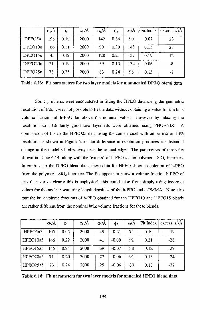
Go/A <!>I Z] ;A GdA <l>z zz/A -Fit Index excess, z*;A
DPE05u 198 0.10 2000 142 0.36 90 0.07 23
DPEOlOu 166 0.11 2000 90 0.30 148 0.13 28
DPE015u 145 0.12 2000 128 0.21 137 0.19 12
DPE020u 71 0.19 2000 59 0.13 134 0.06 -8
DPE025u 73 0.25 2000 83 0.24 98 0.15 -1
'fable 6.13: Fit parameters for two layer models for unanmeaBedllOJIP'EO lbnend data
Some problems were encountered in fitting the HPEO data using the geometric
resolution of 6%, it was not possible to fit the data without obtaining a value for the bulk
volume fraction of h-PEO far above the nominal value. However by relaxing the
resolution to 13% fairly good two layer fits were obtained using PHOENIX. A
comparison of fits to the HPE025 data using the same model with either 6% or 13%
resolution is shown in Figure 6.16, the difference in resolution produces a substantial
change in the modelled reflectivity near the critical edge. The parameters of these fits
shown in Table 6.14, along with the 'excess' of h-PEO at the polymer- Si02 interface.
In contrast to the DPEO blend data, these data for HPEO show a depletion of h-PEO
from the polymer- SiOz interface. The fits appear to show a volume fraction h-PEO of
less than zero - clearly this is unphysical, this could adse from simply using incorrect
values for the nuclear scattering length densities of the h-PEO and d-PMMA. Note also
that the bulk volume fractions of h-PEO obtained for the HPE010 and HPE015 blends
are rather different from the nominal bulk volume fractions for these blends.
Go/A <!>I Zt ;A GdA <l>z zz/A Fit Index excess, z*/A
HPE05a5 105 0.05 2000 49 -0.21 71 0.10 -19
HPE010a5 166 0.22 2000 41 -0.09 91 0.21 -28
HPE015a5 145 0.24 2000 39 -0.07 88 0.12 -27
HPE020a5 71 0.20 2000 27 -0.06 91 0.13 -24
HPE025a5 73 0.24 2000 29 -0.06 89 0.13 -27
Table 6.14: Fit parameters for two layer models for annealed HPEO blend data
194

0.5
.------.. 0::: '---./
9-0.5 01 0 _j
-1.0
-1.5
0.015 0.020 o;,&.-1
······data -6% resolution - - 13% resolution
0.025 0.030
Figure 6.16: Two layer model fits to HPE025 data, these are the same model with
two different resolutions ( 6% and 13% ).
NR Kinetics
Figure 6.17 shows reflectivity data collected from the blends DPE025(u-a6) and
DPE020(u-a6). There is no trend in the reflectivity data with increasing annealing time ,
although the unannealed samples exhibit the lowest reflectivity the reflectivity does not
increase monotonically for the subsequently annealed samples. These reflectivity data
were analysed in the same way as the NR Equilibrium data, again it was found that for
the DPE025 blends VOLFMEM fits with an excess of d-PEO at the air-polymer or Si02
- polymer interface could be obtained.
195

······ DPE020u - ·· DPE020a1 - · - DPE020a2 - - DPE020a.3 -DPE020a4 - - · DPE020a5 -- DPE020a6
IF'igure 6.Jl7a: !Refllectivity dlata for the DIPE020 lbllends, as a fmuction1 of anrnealing
time. Error bars from Poisson statistics irndu..ndled 1for the u.maumealled data.
······ OPE025u -·· OPE025a1 - · - DPE025a2 - -OPE025a3 -DPE025a4 - - · OPE025a5 -- DPE025a6
0.02 0.03 0.04 0.05 0.06 0.07 0/A- 1
Figure 6.Jl7b: Reflectivity data for the DPE025 !blends, as a function of annealing
time. Error bars from Poisson statistics incBuded for the unannealed data.
196

Two layer models were fitted to the data, using PHOENIX, with an excess of d-PEO at
the Si02 - polymer interface and a large air-polymer interfacial roughness. The
parameters of these two layer fits can be found in Table 6.15 along with fit index and the
surface excess, z*si, of d-PEO at the SiOrpolymer interface. For the DPE020 blends the
value of the Si02-polymer surface excess reaches an equilibrium value of 32(5)A. after 1
hour annealing. There surface excess for the DPE025 varies rather more as a function
of annealing time but there seems to be no pattern in the variation, so this may be the
result of unusually large errors in these values. The average value of the surface excess
for the annealed DPE025 is 45(6)A..
0
Zt ;A. adA. Z2/ A Fit Index excess, z * sJ A ao/A 1\lt 1\12
DPE020u 71 0.19 2000 59 0.13 133.6 0.06 -8
DPE020a1 322 0.19 2000 89 0.52 88 0.08 29
DPE020a2 82 0.19 1764 60 0.77 70 0.08 41
DPE020a3 148 0.19 1773 63 0.62 74 0.11 31
DPE020a4 134 0.19 1773 62 0.63 72 0.10 31
DPE020a5 336 0.16 2000 88 0.51 82 0.13 29
DPE020a6 346 0.19 1773 101 0.52 89 0.05 30
DPE025u 73 0.25 2000 83 0.24 98 0.15 -1
DPE025a1 300 0.25 2000 77 0.67 102 0.13 43
DPE025a2 324 0.24 2000 66 0.88 82 0.05 53
DPE025a3 231 0.24 2000 70 0.83 82 0.07 48
DPE025a4 298 0.28 2000 72 0.69 86 0.09 35
DPE025a5 674 0.24 2000 56 0.72 95 0.06 46
DPE025a6 400 0.25 2000 90 0.68 100 0.13 43
Table 6.ll5: Fit parameters for two Bayer models obtained using PHOENIX for the
NR Kinetics data.
197

6.2.3 lDnscussiorn
Although it is possible that swapping the locus of deuteration changes the relative
surface energies of PEO and PMMA to Si02 sufficiently to reverse the enrichment
behaviour. The expectation must be that the effects of deuteration would be far smaller
than the chemical effect. This leads to the conclusion that the composition profiles
obtained from either the DPEO or HPEO blends are inconect. Tentatively it will be
assumed that the DPEO results are conect for the following reasons:
(1) More data has been collected for the DPEO blends and the results are all consistent.
(2) It was not necessary to relax the resolution for DPEO in order to obtain good fits.
(3) The NR data for the HPEO blends intrinsically contain less infonnation than for the
DPEO blends because the critical edge fall at higher Q.
(4) The negative values for the volume fraction of h-PEO at the polymer - Si02
interface.
Clearly this discrepancy also casts some doubt on the validity of the DPEO data and the
solution to this would be to collect more data using other techniques.
Figure 6.18 shows the variation of the excess of d-PEO at the Si02 - polymer
inte1face, z*si. as a function of the bulk volume fraction of d-PEO. The thickness of the
adsorbed layer is of the order of the radius of gyration for the d-PEO ( -lOOA). This is
far thicker than the thickness predicted by mean field theory, using the values of X
obtained in Section 6.1 of this thesis. A selection of theoretical predictions of the surface
composition profile are shown in Figure 6.19, these were calculated using the Jones and
Kramer approximation to the theory of Binder with a value of cJ>s = 0.25 and a range of
values for ~y and X· Data in the literature indicates that ~y, relative to air is quite small
for PEO and PMMA3, around 2 mJ m-2
, and it would seem reasonable to assume that the
difference relative to Si02 would also be small. However even if the surface energy
difference were much larger than that used for the calculations shown in Figure 6.19 the
predicted surface enrichment profile would still be thin compared to the experimental
measurement.
198

0<( "'-.. 40
* N
u) 30 (/) <1) u X
w 20 <1)
u 0 't ::J 10
(f)
+ Data -Linear fit
I
0 ~-L~~~~~~-L~~~~~~~~~~-L~~~~ 0.00 0.05 0.10 0.15 0.20 0.25 0.30
Bulk Volume Fraction DPEO
Figure 6.18: Surface excess of d!-l?IEO at the polymer D Sn02 nnterface as a function
of the lbulk voUume fraction of dl-l?IEO.
0 w o__ I
-I:J:y = 1 mJ m-2, x = -0.018
- -h:y = 1 mJ m~2 • x = -0.009 -·-I::J.-y = 2.5 mJ m-
2, x = -0.018
-··I::J.-y = 2.5 mJ m-, x = -0.009 x DPE025 data
-o
c 0.6 0
+-' u 0 I.....
0.4 4-
<1)
E ::J
-0 0.2 >
50 100 150 200 250 300
Depth /A
Figure 6.19: Model composition versus depth profiles calculated using mean field!
theory, with a selection of X and Ay values.
199

There are two explanations as to why the layer enriched with d-PEO at the Si02 interface
is so much thicker than predicted:
(1) There is a failure in the mean field theory such that it does not predict the thickness
of the surface enriched layer accurately for all systems, there is already some evidence
that this may be the case - it has been observed4 that the shape of the near surface
enrichment profile in d-PS/h-PS deviates slightly from the mean field prediction near the
surface. Deviations from the profile shape predicted by a mean field theory have been
observed in this work for brush formation in d-PS(F)/h-PS blends. Kramer5 reports that
in the d-PEP/h-PEP system a shallow plateau, -50A wide, is observed in the near surface
composition profile.
(2) There may be physical processes that occur in PEO/PMMA blends that are not
accounted for by the mean field theory used here, such as a difference in segmental
volume between the blend components or surface induced crystallisation. However the
blends used in this work were deliberately chosen such that there was no bulk
crystallisation of the of the PEO. The volwne fraction of d-PEO at the Si02 does rise to
values rather higher than those required for bulk crystallisation, but x-ray diffraction
measurements6 show no signs of crystallinity in these thin film samples. However this
absence of observed crystallinity may be because x-ray diffraction is not sensitive enough
to detect the very small fraction of crystallisation that would be required to produce the
observed effect.
One would expect both the PEO and PMMA to interact with the Si02 surface via
hydrogen bonding to silanol groups on the surface7 '8
, the PMMA interacting via the
carbonyl oxygen and the PEO via the ether oxygen. The fact that the PEO is found in
excess at the Si02 surface implies that the ether oxygen has a more negative partial
charge than the carbonyl oxygen.
The large smface roughness of these blends has rendered the analysis of these
data difficult, since it introduces a further unknown parameter in the data analysis and
removes the Kiessig fringes that are useful in fitting the data. Ideally it would be
desirable to repeat these experiments with smoother samples. It was observed during
preliminary experimental work that spun cast films of h-PMMA/d-PMMA were rougher
when cast from chloroform than those cast from toluene, changing the casting solvent
could improve the s<unple roughness, although the blends are still quite rough even after
annealing. This would suggest that the roughness arises when the films make the
transition from being in the melt or solution state - where the sample would be smooth -
200

to the glassy state, whether it arises from further loss of solvent or from cooling to below
the glass transition temperature of the blend. Therefore it may be possible to produce
smoother samples either by slow cooling from the melt or by using a less volatile casting
solvent - the difficulty here is to find a suitable solvent for both PEO and PMMA.
Alternatively these blends could be studied in the melt state using neutron reflectometry,
in order to detennine the composition profile near the air-polymer interface, the
assumption being that in the melt state the blends will be smooth. This would need to be
done under an inert atmosphere to prevent sample oxidation, at present equipment is not
available to do this at CRISP, however there are no difficulties in principle with such an
experiment. An experiment of this sort offers a new line of study; the surface energies of
PEO and PMMA are reported3 to vary at a different rate with temperature, this is
illustrated in Figure 6.20. Tlris means that the difference in surface energy between the
two components of the blend varies as a function of temperature, it would be interesting
to study the surface enrichment behaviour of these blends and probe the effect of this
varying smface energy difference.
45
' N I
E 40
-:l
E ""35 >-01 L Q) c
30 w Q)
u 0
'+- 25 L ::l '
Ul '
20 250 300 350 400 450 500
Temperature /K
Figure 6.20: Values of surface energy (from the literature) for PEO and PMMA,
as a function of temperature.
201

Another advantage of a study at elevated temperature is that, provided the
temperature is kept high enough, bulk Ciystallinity can be avoided even at higher volume
fractions of d-PEO.
The blends used in this work exhibited a substantial amount of off specular
reflectivity, it is possible that this arises from the large roughness of the samples however
the expected off specular reflectivity for such a situation would tend to be more
symmetric about the specular peak9 , in addition the length scale of the roughness - as
measured by contact profilometry is probably rather larger than the coherence length of
the neutrons. Another source of off specular scattering is Yoneda scatter10 which occurs
when incident neutrons although not totally reflected at the sample surface are refracted
on entering the sample such that they are totally reflected just below the sample surface,
again this would tend to lead to an off specular scattering pattern somewhat more
symmetric about the specular peak. The most likely explanation is that the behaviour
observed is due to small angle scattering!! . Tllis must arise from composition
fluctuations, however it is not due to the crystallisation of the d-PEO since no
characteristic peaks are seen in the x-ray diffraction from these films. The violet
iridescence observed in the unannealed DPE020 and DPE025 could also be attributed
to scattering from composition fluctuations, although in this case the length scale of the
composition fluctuations must be much larger (since light has a longer wavelength than
the neutrons used in this work). These concentration fluctuations are much smaller in
the annealed blends, since after annealing the off-specular scatter is much reduced,
although still present and the violet iridescence has gone.
202

!li.2.4l Col!lldusions
The surface composition profiles of annealed d-PEO/h-PMMA blends have been
studied as a function of the bulk volume fraction, <!JB, of d-PEO (with <!>B < 0.30 to avoid
bulk crystallisation). NRA indicated that the distribution of d-PEO in thin films of d
PEO/h-PMMA was unifonn, within the resolution of the technique (-300A). Neutron
reflectometry showed an excess of d-PEO at the Si02-polymer interface. The surface
composition reached a maximum value of 0.70 d-PEO for a blend with <!>B = 0.25, the
characteristic length scale of the profile was around 80A, which is similar in size to the
radius of gyration of the d-PEO. The equilibrium surface excess was reached in less than
one hour annealing at 423K. The fonn of the enrichment profile could not be described
accurately by mean field theory, the theory predicts a vety thin region of smface excess
for blends such as this, with large negative X parameters which are measured elsewhere
in this work for these blends.
The analysis of the neutron reflectometry data was made substantially more
difficult by the presence of a large amount of surface roughness at the air-polymer
interface ( -lOOA), for this reason no definitive statement can be made on the surface
composition profile of these blends at the air-polymer intetface.
This system also provided an excellent practical example of the non-uniqueness
of neutron reflectometry data, initially a model with an excess of d-PEO at the air
polymer interface was fitted, but this model was discounted on the basis of SIMS results
on the same system and the fact that the extreme roughness of the air-polymer interface
will produce a large reduction of the apparent surface volume fraction of d-PEO.
Neutron reflectometry experiments were also done on analogous h-PEO/d
PMMA blends, but it is was not possible to fit the data with physically reasonable
models.
203

6.2.5 !References for Section 6.2
1 . M. Hanshorne, S. Affrossman, unpublished data.
2. P. Sakellariou, Polymer, 34(16), 1993, 3408.
3 . J. Brandrup, E.H. Immergut, 'Polymer Handbook 3rd ed.' J. Wiley & Sons, 1989.
4. R.A.L. Jones, L.J. Norton, E.J. Kramer, R.J. Composto, R.S. Stein, T.P. Russell, A.
Mansour, A. Karim, G.P. Felcher, M.H. Rafailovich, J. Sokolov, X. Zhao, S.A. Schwarz,
Europhysics Letters, 12(1), ll990, 41.
5 . E.J. Kramer, unpublished data.
6. R.W. Richards, unpublished data.
7 . J. Rubio, J.A. Kitchener, Journal of Colloid and InteJface Science, 57(1), 1976,
132.
8 . H.E. Johnson, S. Granick, Macromolecules, 23, 1990, 3367.
9. C.A. Lucas, Faraday Disscussion, 89, ll990, 928.
10. Y. Yoneda, Physical ReviewB, 131,1963,2010.
11 . C.J. Clarke, private communication.
204

This page left intentionally blank
205

7. 1 Experimen~al
The composition depth profiles, <j>(z), of a series of mixtures of end functionalised
deuterated polystyrene with hydrogenous polystyrene have been detennined. The
deuterated polystyrene was end capped with a small perfluorinated group at one (d
PS(F)) or both (d-PS(F2)) ends or had no fluorinated end caps (d-PS). Details of the
end group can be found in Section 4.1.1. The molecular weights and 'global' sample
codes of the polymers used in this section can be found in Table 7.1. Both Nuclear
Reaction Analysis (NRA) and Neutron Reflectometry (NR) were used in this work,
details of the experimental procedure can be found in sections 4.3 and 4.4 respectively.
NR data were collected using the multidetector (April 1994) and the single detector
(November 1993).
Global Code Mw
d-PS(F) TK92 658,000
h-PS TK58 1,710,000
d-PS TK93 816,000
d-PS(F) TK89 30,700
h-PS TK79 44,700
d-PS(F2) TK145 56,000
Table 7.1: Details of the polymers used in this section.
The experiments carried out on these blends can be divided into six parts, these can be
summarised as follows:
(1) High Mw d-PS(F)/h-PS blends, equilibrium behaviour- 'Equilibrium (1)'
(2) High Mw d-PS/h-PS blends, equilibrium behaviour- 'Equilibrium (2)'
(3) Low Mw d-PS(F)/h-PS blends, equilibrium behaviour- 'Equilibrium (3)'
(4) Low Mw d-PS(F)!h-PS blends, influence of casting solution concentration on initial
composition gradients- 'Casting Concentration'
206
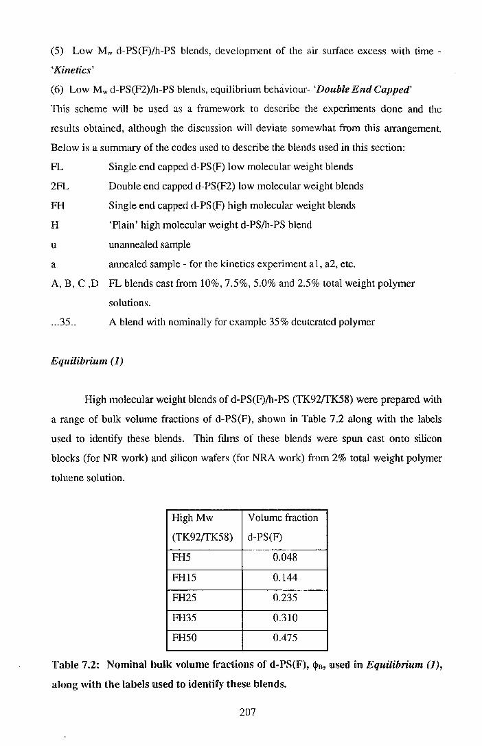
(5) Low Mw d-PS(F)/h-PS blends, development of the air surface excess with time -
'Kinetics'
(6) Low Mw d-PS(F2)/h-PS blends, equilibrium beluiviour- 'Double End Capped'
This scheme will be used as a framework to describe the experiments done and the
results obtained, although the discussion will deviate somewhat from this arrangement.
Below is a summary of the codes used to describe the blends used in this section:
FL Single end capped d-PS(F) low molecular weight blends
2FL Double end capped d-PS(F2) low molecular weight blends
FH Single end capped d-PS(F) high molecular weight blends
H 'Plain' high molecular weight d-PS/h-PS blend
u unannealed sample
a annealed sample - for the kinetics experiment al, a2, etc.
A, B, C ,D FL blends cast from 10%, 7.5%, 5.0% and 2.5% total weight polymer
solutions .
... 35.. A blend with nominally for example 35% deuterated polymer
Equilibrium (1)
High molecular weight blends of d-PS(F)/h-PS (TK92{fK58) were prepared with
a range of bulk volume fractions of d-PS(F), shown in Table 7.2 along with the labels
used to identify these blends. Thin films of these blends were spun cast onto silicon
blocks (for NR work) and silicon wafers (for NRA work) from 2% total weight polymer
toluene solution.
HighMw Volume fraction
(TK92{fK58) d-PS(F)
FH5 0.048
FH15 0.144
FH25 0.235
FH35 0.310
FH50 0.475
Table 7.2: Nominan bulk volume fractions of d-PS(F), ljln, used in Equilibrium (1),
anong with the labels used to identify these blends.
207

The average thickness of the films used for NRA was 2000±250A and for NR samples
the average thickness was 1400±100A, measured by contact profilometry. l11is
difference in thickness arises from a difference in the spinning speed used in casting
(2000 rpm ancl4000 rpm respectively). Thinner films were prepared for the NR work in
order that Kiessig fringes, characteristic of the sample thickness, could be seen in the
reflectivity data. Slightly thicker films were prepared from for the NRA work in order
the air and silicon intedaces could be clearly resolved. Unannealed films were retained
and films annealed under vacuum for 10.8 days at 428K were also prepared. Secondary
ion mass spectrometry (SIMS) by collaborators at Strathclyde University has shown that
after this annealing programme the smface volume fraction of d-PS(F) has reached an
equilibrium value1• NRA measurements were made on blends FH5, FH15, FH25, FH35
and FH50 on a single occasion in November 1993, NR measurements were made on
FH5, FH25, FH35 and FH50 on a single occasion in November 1993.
Equilibrium (2)
High molecular weight blends of d-PS/h-PS (TK93/TK58) were prepared with
compositions shown in Table 7 .3. Thin films of these blends were spun cast onto silicon
wafers from -4% total weight polymer toluene solution (spinning speed 4000 rpm). The
average film thickness measured by contact profilometry was 2500±500A. These
samples were annealed for 9.9 days at 428K. NRA measurements were made on a single
occasion in March 1994. The intention of these experiments was to obtain a measure of
the contribution that sutface enrichment made to the behaviour seen in 'Equilibrium
(1)'.
High Mw Volume fraction
(TK93/TK58) d-PS
H5 0.045
H15 0.141
H25 0.233
Table 7.3: Nominal bulk volume fractions of d-PS, <l>n, used in Equilibrium (1),
along with the labels used to identify these blends.
208

Equilibrium (3)
Low molecular weight blends of d-PS(F)/h-PS (TK89{fK79) were prepared with
a range of bulk volume fractions of d-PS(F), see Table 7 .4. Thill films of these blends
were spun cast onto silicon blocks (for NR) and silicon wafers (for NRA), from 7.5%
solution of total polymer in toluene (spinning speed 2000 rpm). The average thicknesses
of the films produced were 3900±200A and 3750±250A respectively, measured by
contact profilometry. Thicker films were used for the low molecular weight blends in
this experiment than the high molecular weight blends in Equilibrium (1) because it was
found that for thinner films (annealed at higher temperatures) the film completely
dewetted from the silicon substrate, such dewetting behaviour has been investigated by
other workers2• Unannealed films were retained and films annealed under vacuum for 2
days at 403K were also prepared, SIMS results have shown that after this annealing
programme the surface volume fraction of d-PS(F) has reached an equilibrium value.
LowMw Volume fraction
(TK89{fK79) d-PS(F)
FL5 0.046
FL10 0.091
FL15 0.138
FL20 0.190
FL25 0.248
FL35 0.331
FL50 0.504
Table 7.4: Nominal bulk volume fractions of d-PS(F), <!Jn, used in Equilibrium (3),
along with the labels used to identify these blends.
NRA measurements were made on a single occasion in November 1993. NR
measurements were made on two occasions, in November 1993 (FL5, FL25, FL50) and
April 1994 (FL10, FL15, FL20 and FL35).
209

Casting Concentration
To observe the effect that the concentration of the casting solution had on the
near surface composition profile of unannealed samples four solutions of a low molecular
weight d-PS(F)/h-PS (TK89!fK79) blend were prepared. The volume fraction of d
PS(F) was fixed at 0.331, solutions with weight percentage of total polymer 10%, 7.5%,
5% and 2.5% were made. These samples will be refened to as A35u, B35u, C35u and
D35u respectively. These solutions were spun cast onto silicon blocks, spinning speed
was 2000rpm. Film thickness for these samples, measured using contact profllometry
were: 5820±30A, 3870±20A, 1430±10A and 620±30A respectively. NR experiments
were cruried out on these films on a single occasion in April 1994.
Kinetics
To evaluate the kinetics of the fonnation of the air surface excess of d-PS(F)
observed for the low molecular weight d-PS(F)/h-PS (TK89!fK79) a series of samples
were prepared, all with bulk volume fraction of d-PS(F) of 0.331. The sample
preparation procedure was identical to that used in Equilibrium (3). Average film
thicknesses for these sample was 3870±20A. An unannealed sample was retained and
srunples annealed under vacuum at 403K were prepared, the annealing times used and
the corresponding sample labels ru·e shown in Table 7.5.
Annealing time /hours
FL35u 0
FL35a1 0.33
FL35a2 1
FL35a3 3
FL35a4 5
FL35a5 48
Table 7.5: Annealing times and! sampDe labels for the low molecular weight blends
used in the Kinetics.
NR measurements were made in April 1994, one sample (FL35a2) was measured on a
different date by the CRISP instrument scientists using the single detector.
210

Double End Capped
Low molecular weight blends of the double end capped d-PS(F2) with h-PS
(TK145{fK79) were prepared, the compositions of the blends used can be found in
Table 7.6.
LowMw Volume fraction
TK145{fK79 d-PS(F2)
2FL10 0.094
2FL35 0.335
2FL50 0.486
Table 7.6: Nominal buUk volume fractions of d-IPS(F2), <j>8 , used in Double End
Capped, aHong witlh the Ualbels u.nsed to idlentify tlhese !blends.
Thin films of these blends were spun cast onto silicon blocks (for NR) from 5% total
weight polymer toluene solution (spinning speed 2000 rpm). The average thickness of
these blends, measured using contact profilometry, was 2220±40A. An unannealed
sample (2FL35u) was retained, in addition samples of all three blends were annealed
under vacuum for 2 days at 403K. NR data were collected on a single occasion in April
1994.
211

7.2 ResuUs
Before presenting the results a number of general observations regarding data
analysis will be made.
Comments on Neutron Reflectometry
Three methods of data analysis were used on the reflectivity data:
(1) VOLFMEM, described in Section 4.3.3., was used to fit 'free form' composition
profiles, <j>(z), with a pixel resolution in the range lOA - 15A and internal smoothing of
lOOA.
(2) PHOENIX, described in Section 4.3.3., was used to fit multilayer models (up to 3
layers) with Gaussian roughness between the layers.
(3) PHOENIX was used to fit profiles with a Tanh function (see Equation 7.1) to
describe composition profiles at the air and/or silicon interface.
Equation 7.1
<j> 1 corresponds crudely to a 'surface composition', Zoff and w approximate to the offset of
the decay to bulk composition, <J>s, and the sharpness of the decay, respectively. For the
fits using PHOENIX the roughness at the air and silicon interfaces was fixed at 5A and a
15A Si02 layer was included, although this improved the quality of the fits for the thinner
samples (in line with the calculation presented in section 3.1.2), the parameters fitted
were essentially the same as those obtained with no SiOz layer. The experimental
resolution used in the fitting procedures was fixed at the geometric value (3.5% and
4.4% for the November 1993 and April 1994 experiments respectively). The fit
parameters from the PHOENIX fits are quoted along with the 'Fit Index', which is not
identical to the nonnalised X2 parameter traditionally used. The Fit Index is defined in
section 4.3.3. As a guide the nonnalised X2 parameter was calculated for a limited
number of multilayer fits to the reflectivity data, compruisons of these values with the
equivalent fit index can be found in Table 7.7.
212

Blend Fit Index nonnalised X2
2FL10a 0.06 4
FL35u 0.10 8
FL50a 0.16 17
FH35a 0.15 19
1l'albDe 7. 7: Corresponullence between the Fit mdex and the no~rmallnsed X2
parameteir for sellededl bllend.s (muRtiHayer fits).
The <)l(z) profiles generated using VOLFMEM all show a sharp decrease in the
volume fraction of d-PS(F) in the top 30A of the films (see Figure 7.1). This behaviour
was particularly noticeable in the low molecular weight blends. This decrease in <)l(z) is
an artefact of the maximum entropy data analysis.
1.0 ,........._ N LL
L 0 0.8
LL ......__., (/) ()_
0.6 I -a c 0
+-' 0.4 u 0 L
'+-
E o.2 ::J
0 >
oo
0 0
0
0
+
0
0
0 2FL35a 1:!. FH25a + FL35a
0
+
++++++++++++++++++++++++++
o.oW-~~~~~~~~~~~~~~~~~~~~
0 100 200 300 400 500 Depth /A
Figure 7.].: A selection of <jl(z) profiles, generated using VOLIFMEM, inlustrating
the downturn in <)! at the surface.
Firstly VOLFMEM does not include a value for the air/surface roughness. To
compensate for this it would be expected that the maximum entropy algorithm would
213

reduce the volume fraction of the surface layers to mimic the effect of roughness.
Secondly the tnmcation of the R(Q) data at finite values of Q introduces further
artefacts. To evaluate the influence of these effects 'simulated' R(Q) data were created
from a Tanh profile (<j>1 = 0.63, <l>B = 0.25, Zoff = 33.5 and w = 120, film thickness 4000A,
'experimental' resolution = 4.4% ), with air- polymer and polymer - silicon roughness' of
5A, simulated error values were included. The simulated reflectivity data were analysed
by VOLFMEM in a manner identical to that used for real data. A comparison of the
'real' profile and the profiles extracted using VOLFMEM and PHOENIX (Tanh model)
are shown in Figure 7 .2.
0.6
0.5
c 0 0.4
-+-' u 0 L
'+- 0.3 Q.)
E ::l
0.2 0 >
0.1
0.0 0 200
-Original 0 VOLFMEM
- -PHOENIX (Tanh
400 Depth /A
600 800
Figure 7.2: Comparison of composition profiles produced by PHOENIX (Tanh
model) and VOLFMEM from simulated data.
The simulated data were also fitted with multilayer and Tanh models. A comparison of
the smface excess, z*, (given by Equation 7.2) and surface volume fraction of d-PS(F),
<Pair. obtained using these three methods and from the original <J>(z) profile are shown in
Table 7.8.
Equation 7.2
214
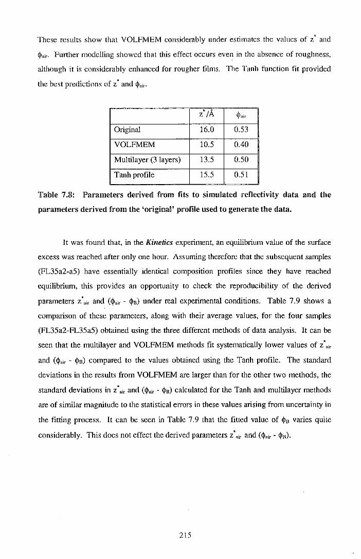
These results show that VOLFMEM considerably under estimates the values of z* and
<l>air· Further modelling showed that this effect occurs even in the absence of roughness,
although it is considerably enhanced for rougher films. The Tanh function fit provided
the best predictions of z * and <l>air·
z* /A <I> air
Original 16.0 0.53
VOLFMEM 10.5 0.40
Multilayer (3 layers) 13.5 0.50
Tanh profile 15.5 0.51
'fable 7.8: Parameters derived! from fits to snmuHatedl reflectivity data allldl the
parameters derived from the 'original' profile used to generate the data.
It was found that, in the Kinetics experiment, an equilibrium value of the surface
excess was reached after only one hour. Assuming therefore that the subsequent samples
(FL35a2-a5) have essentially identical composition profiles since they have reached
equilibrium, this provides an opportunity to check the reproducibility of the derived
parameters z • air and ( <l>air - $B) under real experimental conditions. Table 7. 9 shows a
comparison of these parameters, along with their average values, for the four samples
(FL35a2-FL35a5) obtained using the three different methods of data analysis. It can be
seen that the multilayer and VOLFMEM methods fit systematically lower values of z*air
and ($air - $13) compared to the values obtained using the Tanh profile. The standard
deviations in the results from VOLFMEM are larger than for the other two methods, the
standard deviations in z\ir and (<l>air- $B) calculated for the Tanh and multilayer methods
are of similar magnitude to the statistical errors in these values arising from uncertainty in
the fitting process. It can be seen in Table 7.9 that the fitted value of <I>B varies quite
considerably. This does not effect the derived parameters z*air and ($air- $B).
215

FL35a2 FL35a3 FL35a4 FL35a5 Average
VOLFMEM * 40 27 23 30 30 ± 7 Z air
<!>B 0.36 0.35 0.36 0.35 0.36 ± 0.01
<!>air- <J>B 0.48 0.38 0.35 0.40 0.40 ± 0.06
Multilayer * 32 29 31 28 30 ±2 Z air
<j>B 0.37 0.32 0.29 0.36 0.34 ± 0.04
<!>air- <J>B 0.39 0.41 0.43 0.35 0.40 ± 0.03
Tanh * 35 36 33 38 36 ±2 Z air
$n 0.35 0.28 0.28 0.30 0.34 ± 0.03
<!>air- $B 0.45 0.52 0.43 0.47 0.47 ± 0.04
'fable 7.9: Comparison of parameters obtained! using the tlhree methods of data
analysis, from four identical sampRes. lErrors are standard deviations.
The average volume fraction of d-PS(F), $av. is defined below:
<j> av = 7 J $ (z)dz
Equation 7.3
(where 1 is the film thickness).
<l>av was calculated using all three methods of data analysis for all the films used and it
was found that the values obtained were up to 0.05 below the nominal value of $av.
calculated from the masses of d-PS(F) and h-PS used in making the blends. The cause of
this discrepancy is not clear, but it may be due to enors in the values of the nuclear
scattering length densities used for h-PS and d-PS or to a mixture of systematic and
random enors in detennining Q. Since the effect is small and does not effect the values
of z*air and ($air- $n), which will be used in the discussion, it was not investigated further.
The data were initially analysed using VOLFMEM, and Tanh profiles were
subsequently fitted to the reflectivity data using starting parameter values derived from
the <j>(z) profiles generated by VOLFMEM. It is the parameters derived from the Tanh
profiles that most accurately represent the probable distribution of d-PS(F) in the films
and will be used in the discussion. The exception to this is the analysis of the unannealecl
216

samples, where a depletion layer was seen below the smface excess, see Figure 7.3 for a
schematic illustration, in this case multilayer fits were used to evaluate the extent of the
depletion z * dep· Statistical errors in the surface excess (measured by neutron
reflectometry) and the surface volume fraction are ±2A and ±0.02, respectively.
c 0
+-' 0 0 L
LL
Q)
E ::J
0 >
---------------------------------------------------- $air
Depth
Figure 7.3: Schematic diagram of structure observed in unanneaBed films, with
definntions of terms used!.
Comments on Nuclear Reaction Analysis
The surface excesses z* were calculated from the NRA data using GENPLOT;
the average bulk volume fraction, $s, was subtracted from the normalised data. This
'bulk subtracted' data was then numerically integrated to give the surface excess. This
value of the excess was found to be significantly lower than the value measured using
neutron reflectometry, this discrepancy arises from resolution effects, which will be
discussed here. Figure 7.4 illustrates the effect of convoluting a Gaussian resolution
function (Full Width Half Maximum (FHWM = 350A), with a series of step functions.
217

0.7
0.6
c 0.5 0
+-' u 0 0.4 L ...__
(]) 0.3 E
::::J -0
0.2 >
0.1
0.0 --400-200 0 200 400
Depth /A
-300..&. layer - - 200.&. layer - . - 1 oo.&. layer · · · · · · 75'A layer -··50.&. layer
600 800 1000
!Fig!Ure 7.4: Severan step fu.mctnol!lls wfiUn varying thickness (cpa~r = 0.7) convoRuded
with a Gaussian resoDution function (IFWIHIM = 350 A).
These step functions have a thin layer with a volume fraction 0.7 sandwiched between
'air' and a thick layer with bulk volume fraction = 0.2. The thickness of the overlayer is
varied from 50A - 300A, i.e. 0.15 FWHM to 0.85 FWHM. The values of z* and the
'surface volume fraction', cpair measured for these simulated profiles using the methods
applied to the experimental data are shown in Table 7.1 0, along with the excess
calculated for the original step function. For the NRA data cpair is taken to be the
maximum measured value of cp in the region near the surface.
Overlayer thickness/ A original z*/A measured z*/A measured cpair
300 150 113 0.51
200 100 65 0.41
100 50 20 0.28
75 38 10 0.24
50 25 3 0.22
'falble 7.TI.O: !Reduction in tille value of z* measured by NRA comJPared to the
original z*.
218

The resolution effect causes decreases in the measured z * and <Pair that are of the
magnitude required to explain the differences in values obtained using neutron
reflectomet:ry and nuclear reaction analysis. In real experiments the measured value of z*
would also depend to a cettain extent on the shape of the near surface composition
profile. There are a number of procedures which could be adopted in order to extract
the 'true' z * from the NRA data:
(a) In principle Fourier transform deconvolution of the NRA data could be performed,
this would involve Fourier transfonning the measured <)l(z) and dividing by the Fourier
transform of the resolution function and then Fourier transfonning the resulting function
to obtain a deconvoluted <)l(z) from which the 'true' z* could be extracted. More details
of this procedure can be found in reference 3 . Tins procedure would be sensitive to
statistical eiTors in the measured <)l(z) and inadequate knowledge of the resolution
function.
(b) The experimental data could be fitted with a model <)l(z) convoluted with a resolution
function. This would be computationally demanding, but rather more robust than (a).
(c) The measured z* could be multiplied by a 'correction factor' derived from data such
as that in Table 7.10, although the correction factor would be somewhat arbitrary
because it depends on the profile shape.
Rather than using these procedures on the NRA data, it can be shown that the
NR and NRA data are comparable by taking the Tanh function profiles fitted to the NR
data and convoluting them with a Gaussian resolution function and then comparing these
convoluted NR data with the NRA data. The compruisons between <Pair and the surface
excess, z*, obtained in this way can be found in Figure 7.5 for the FH (Equilibrium (1))
blends and Figure 7.6, the FL (Equilibrium (3)) blends. The Gaussian resolution
function for these data had a FWHM of 300A for both sets of data, this value was found
to give the best fit and is in line with the expected value. The agreement between the <Pair
obtained using NRA and convoluted NR is very good, but there is rather more scatter in
the z* values. Tills is because the z* calculated using NRA is .quite sensitive to the value
of <)!B chosen when making the integration. (These data will be fully introduced shortly).
219

.~ 0
-e-
0.8
0.6
0.4
0.2
0 Convoluted NR data ~ NRA data
0
0 A
0 A
lFigure /.Sa: Comparnsolll !between cpair values obtained for the JFJH[ lblends IUISnng
NJRA allld NJR l'anlll profnles convohntedl witlhl a Gaussian resollutfion fullllctnmn
(lFWJHIM = 300A).
100 I I I I
0 Convoluted NR data ~ NRA data
80 1- -
A 0 0
60 1- -A
0<( A
~ .. N 0
40 t- -
20 It> -A
lFigure 7.51b: Comparison between z* values obtained for the FH blends using NRA
and NR. Tanh profiles convoluted with a Gaussian resolution function (FWHM =
300A).
220

0.6
0 Convoluted NR dota 6. NRA data d 0
0.5
0.4 d
0
'-
~60.3 d
0.2 0 d
0
0.1 ~~.o
0.0 0.0 0.1 0.2 0.3 0.4 0.5 0.6
cPs
Figure 7.6a: Comparison between $a1r vanues obtained! for tlhe FlL blendls using
NRA and NR 'fanh profnles convonuted with a Gaussian resolution function
(FWHM = 300A).
30
0 Convoluted NR data
25 6. NRA data
20 A
ex(
~ 15 * N
d
10 0
0 A
0
A
5 a 0
0 0.0 0.1 0.2 0.3 0.4 0.5 0.6
cPs
Figm·e 7.5a: Comparison between z• values obtained for the FL blends using NRA
and NR Tanh profiles convoluted with a Gaussian r·esolution function (FWHM =
300A).
221

Equilibrium (1)
Composition versus depth profiles for the high molecular weight d-PS(F)/h-PS
blends were obtained from the NRA data using the methods outlined in section 4.4. The
average value for the film thickness, calculated for all these films is 1980±160A, which is
in good agreement with the value obtained by contact profilometry. Figure 7.7 shows
these profiles for samples (a) before annealing and (b,c) after annealing.
0.7
'G:' 0.6 .....___., (f) Q_ I 0.5
-o
c 0.4 0
+-' u 0 0.3 L
4-
([)
0.2 E :::J -0
0.1 >
0.0 0 500 1000
Depth /A 1500 2000
Figure 7.7a: Compositions profiles cjl(z) for tmannealed F.IHI. blends, obtained using
NRA, error bars from Poisson statistics.
These data show that before annealing the d-PS(F) is distributed unifonnly in the
films. After annealing d-PS(F) is found to segregate to both the air and silicon interfaces.
The values of z\ir, z*si and c!>B calculated from the NRA data using GENPLOT are shown
in Table 7.11, the experimental error in the surface excesses is lOA.
222

r---. lL 0.5 ~
(/) Q_
I -o 0.4
c 0
+..J 0.3 0 0 L 4-
Q) 0.2 E :J
.g 0.1
0 0
0
0
0
0
00
0 0
500
0 FH35a D. FH20a + FH5a
1000 Depth /A
0 0 0 0
0 0
0 0 0 0 o o0
0
1500 2000
!Figure 'i.'ib: Composntion profiles for anneaBed IFJHI blends, obtained using NRA.
Enor !bars from Poisso~rn cmmting statistics for a representatnve dataset.
0.8
r---. 0 LL ~
(/) 0.6 Q_
I 0
-o c 0
0 +..J 0.4 0 0 L 4-
Q)
E 0.2 :J -0 >
0.0 0
0 0
0
0
0 0
500
0 FH50a b. FH25a + FH15a
1000 Depth /A
0
0
r::j::Po
0 0 0
0
1500 2000
Figure 'i.'ic: Composition profiles for annealed FH blends, obtained using NRA.
Error bars from Poisson statistics for a representative dataset.
223

Blend <!>n z*air/A z*,J A <Pair <Psi
FH5a 0.04 10 5 0.08 0.06
FH15a 0.14 15 9 0.20 0.18
FH20a 0.18 54 12 0.35 0.49
FH25a 0.22 58 22 0.38 0.31
FH35a 0.28 65 28 0.51 0.40
FH50a 0.45 67 44 0.69 0.60
Table 7.11: Parameters for the FH annealed blends from NRA measurements
The ratio z\i I z*air is 0.5 ± 0.2 for these blends. Values of the maximum volume fraction
of d-PS(F) observed at air (<!>air) and silicon (<!>si) interfaces are also shown in Table 7.11,
the ratio <Psi I <!>air is 0. 9 ± 0.2.
Turning to the NR data, examples of the reflectivity data, R(Q), are shown in
Figure 7 .8a along with fits obtained using PHOENIX (Tanh model), the data exhibit
Kiessig fringes which give an indication of the film thickness. For the blends FH25,
FH35 and FH50 there is a significant increase in the overall reflectivity on annealing, the
FH5 blend shows only small changes in reflectivity on annealing. This is illustrated in
Figure 7.8b. The average value of the film thickness fitted was 1430±100A which is in
good agreement with the values obtained using contact profilometry. Figure 7.9a shows
the composition profiles obtained for the unannealed FH blends using VOLFMEM,
Tanh function profiles were not fitted to these data. Figure 7.9b shows the <j>(z) profiles
obtained for the annealed blends using VOLFMEM and PHOENIX (Tanh model) fits.
The blends FH50u and ~H25u showed a small depletion of d-PS(F) from the air interface
and the blends FH35u and FH5u showed a small excess of d-PS(F) at the air interface.
These deviations from uniformity are very small when compared with the excesses
observed after annealing. The annealed blends all show substantial excesses of d-PS(F)
at both the air and silicon interfaces, the film thickness is small so these excesses lead to a
significant reduction of the volume fraction of d-PS(F) in the middle of the film from the
nominal 'bulk' value. For the NRA experiments the films were thicker and so a weaker
effect of this sort was observed.
224

-6 -
-8
0.00 0.02 0.04 0.06 o;A.-1
··· ·· FH50o 0 FH35a 6. FH25a x FH5a
0.08 0.10
lFngmre 7.8a: Neutron reflectivity data for anneaHedl lFlHI lbRenuls (symbols), wWh fits
from IPHOlENlfX (Tanlh modeR). Error bars for lFH5a from !Poisson statistics.
Successive profiles offset by -1 for clarity.
-2 ,.........._ 0::: ..........-8-4
(J'l
0 __j
-6
-8
0.00
-FH50a - ·· FH50u - -FH5a - · -FH5u
0.02 0.04 0.06 0.08 0.10 o;A.-1
Figure 7.8b: Neutron reflectivity data for umumealed and annealed lFH5 and
lFHSO data, FR-IIS data offset by -1 for clarity.
225

0.6
,........... LL 0.5 .......__, (/) Q_
I """0 0.4
c 0
+-' 0.3 0 0 L 4-
<1) 0.2
E ::::l -0 0.1 >
0.0
)( )( )( )(
0 500 1000
Depth /A
0 FH50u t:::. FH35u + FH25u x FH5u
1500
Figure 7.9a: Composition profiles for umanmealed FH lbiends obtained using
VOJLFMJEM analysis of 1t11eutron reflectivity data.
,.....--.. LL .......__, (/) Q_
I """0
c 0
+-' 0 0 L
4-
<1)
E ::::l -0 >
0.8
0.6
0.4
0.2
0.0 0 500 1000
Depth /A
0 FH5a t:.. FH25a + FH35a x FH50a
1500
Figure 7.9b: Composition profiles for annealed FH blends, calculated from
reflectivity data, VOLFMEM (symbols) and PHOENIX (Tanh model) (solid lines)
fits.
226

Table 7.12 shows the values of the smface excesses z*air and z\i and surface
volume fractions of d-PS(F), <!>air and <l>si, obtai.ned using Tanh profile fits. The ratio z*si I
z*air is 0.75 ± 0.07 and the ratio <!>,i I <!>air is 0.7 ± 0.2. The parameters for the Tanh profile
fits are in Table 7 .13.
Blend <I>B z*air ;A z*,i ;A <I> air <l>si
FH5a 0.01 29 23 0.16 0.08
FH25a 0.13 73 51 0.44 0.38
FH35a 0.16 97 67 0.60 0.48
FH50a 0.32 109 90 0.77 0.62
1'able 7.12: Parameters dernved for the FH annealed blends from Tanh profile fits
to NR data.
Air Silicon
Sample <I>B l!A <I> I Zoff /A w/A <1>1 Zoff /A w/A Fit Index
FH5a 0.01 1600 0.20 129 386 0.095 241 591 0.19
FH25a 0.13 1400 0.54 142 500 0.5 89 489 0.13
FH35a 0.16 1380 0.67 175 387 0.59 120 464 0.13
FH50a 0.32 1304 0.84 214 445 0.63 326 304 0.15
Table 7.13: Parameters for Tanh fits to FH annealed blends.
Equilibrium (2)
Figure 7.10 shows composition profiles obtained from NRA data for the blends
H5a, H15a and H25a. The average thickness measured from these data is 1900±200A,
which is lower than the average value obtained from contact profilometry, this
discrepancy is due mainly to the H5a sample. In common with the high molecular weight
d-PS(F)/h-PS blends segregation is observed at both the air and silicon interfaces.
Values z*5;, z*air, <!>air and <l>si for these blends can be found in Table 7.14. The ratio z*si I
z*air is 0.5 for these data and <l>si I <!>air is 0.5 (excluding the H5a blend). The surface
excesses for these blends are approximately half that of the equivalent end labelled (FH)
blends.
227

Blend QlB z*air ;A z*si /A $air Qlsi
H5a 0.05 2 0 0.06 0.05
H15a 0.15 11 5 0.44 0.19
H25a 0.25 21 12 0.60 0.32
'falblle 7.14: Parameters dernved for tlhe aBllneafied lHI lbiernds lfrom NJRA dlata
,.-.... lL '--"' (f) 0... 0.3 I
\J
c 0
:;::; 0.2 ()
0 L -<1)
~ 0.1 0 >
0 1000 1500 2000 Depth /A
!Figure 7.10: Compositions profiles for annealed! lHl blends, obtained using NRA,
error bars from Poisson statistics.
228

Equilibrium (3)
Figure 7.11 shows <j>(z) profiles for the low molecular weight d-PS(F)/h-PS
blends, obtained using NRA (a) before and (b) after annealing. The average film
thickness indicated by these data appears to be around 2500A, this is significantly less
than the 3750±250A measured using contact profilometry, but there is no clear 'back
edge' visible in the data as there was for the thinner films used for the high molecular
weight blends. This suggest that the incident 3He+ did not penetrate to the silicon
interface, the path length to the silicon interface for the incident angle used is around
1.5~-tm, which is similar in magnitude to the expected stopping distance for 3He+ in
polystyrene. This means no infonnation is available on the composition profile at the
silicon interface.
The NRA data shows the d-PS(F) to be distributed unifonnly in the unannealed
films, in the annealed films there is a small excess of d-PS(F) at the air interface. The air
surface excess, z*air, and the surface volume fraction of d-PS(F), <!>air. for these blends can
be found in Table 7 .14.
0.7
L2' 0.6 '--"' (f)
9- 0.5 -o c 0.4 0
+-' u 0 0 . .3 L
'+-
Q)
0.2 E :J -0
0.1 >
0.0 0 500 1000 1500 2000
Depth /A 2500 .3000
Figure 7.11a: Composition profiles for unannealed FL blends, obtained using
NRA, error bars from Poisson statistics for representative datasets.
229

0.7
l2 0.6 "'----" (!)
9- 0.5 ""0
c 0.4 }++ 0 ++
-+-' u + 0 0.3 "-
'+-
Q) 0.2 E
::J -0
0.1 >
0. 0 L-1.......1.-J'--'--'--''--L..-'--''--L.....I.--J.'--L....L-.L-'-.1-J..--l-.I.-.L.--l-.L......L.--L
0 500 1 000 1500 2000 2500 3000
Depth /A
Figunre 7.Hb: Compositiolll profnles for anmeaRedl FlL blends, obtained using NIRA.
Error bars from !Poisson statistics for representative datasets.
~B z*air ;A ~air
FL5a 0.04 6 0.07
FL15a 0.14 9 0.19
FL25a 0.21 11 0.26
FL35a 0.33 20 0.40
FL50a 0.48 8 0.52
Table 7.14: Parameters derived! for annealed FL blends from NRA data
Figure 7.12a shows examples of the reflectivity data obtained for these samples
along with fits obtained using PHOENIX (Tanh model). For all but the FL5 blend there
is an increase in reflectivity for the annealed samples, this is shown in Figure 7 .12b.
None of the data exhibit fringes characteristic of the film thickness, because the film
thickness is sufficiently large that the fringes are too closely spaced to be resolved. This
means that the reflectivity is insensitive to the film thickness and for this reason the
thickness of the films was set at the value indicated by the contact profilometry.
230

0
-2
,--.... 0:::
"----" ~ -4
Ol 0 _j
-6
-8
0.00 0.02 0.04 0.06 a;fi.-1
······ FL50a 0 FL20a £:. FL1 Oa x FL5a
0.08 0.10
Figure 7.:R.2a: Neutron reflectivity profiles for selected anBlleaHed IF'IL bHendls.
Experimental data (symbols) and J?JHIOJENKX (Tanh modleH) (solid Hine) fnts.
Successive datasets offset by -1 for clarity. lError bars for JFIL5a from l?onsson
statistics.
0
-2
,........., 0:::
-..___;
~ -4 01 0
__j
-6
-8
0.00
-FLSOa -·· FLSOu -- FL35a - -· FL35u - -FL5a - · -FLSu
0.02 0.04 0.06 0.08 0.10 o;A.-,
Figure 7.12b: Neutron reflectivity profiles for the FLS, FJL35 and JFLSO blends
before and after annealing, JFL5 and IF'IL35 data offset by -2 and -1 respectiveny.
231

Figure 7.13 shows composition depth profiles, cjl(z), extracted from the reflectivity data
using VGLFMEM and PHOENIX (Tanh model). Table 7.15 shows values for z*air and
cJlair obtained using the Tanh profile fits, (both before and after annealing). Table 7.16
shows the parameters of the Tanh profile fits.
0.8
..........._ LL .....__.. (/) 0.6 Q_
I u
c 0
+-' u 0 L.
'+--
<1)
E :::)
0.2
0 >
0.0 0 100 200 300
Depth /A
0 FL5a 6. FL1 Oa + FL20a x FL35a ¢ FL50a
400 500
Fngmre 7.13: ComposiHon profi!es for annealed FL blends, obtained from NR.
Symbols a VOLFMEM fits, solid lines- corresponding PHOENIX (Tanh model) fit.
Unannealed Annealed
$s z*air!A $air $s z*arr/A $air
FL5 0.05 9 0.21 0.05 9 0.21
FL10 - - - 0.08 20 0.36
FL15 - - - 0.11 21 0.46
FL20 - - - 0.17 27 0.56
FL25 0.18 15 0.43 0.18 30 0.54
FL35 0.29 17 0.60 0.30 36 0.77
FL50 0.50 12 0.63 0.50 26 0.75
Table 7.15: Parameters derived for FL blends using Tanh models to NR data.
232

<l>s 1/A <!J, Zoff/A w/A Fit Index
FL5u 0.05 4000 0.21 58 50 0.13
FL5a 0.05 4000 0.21 56 49 0.15
FL10a 0.08 4000 0.37 68 55 0.13
FL15a 0.11 4000 0.49 55 85 0.10
FL20a 0.17 4000 0.57 64 78 0.08
FL25u 0.18 3818 0.45 52 79 0.15
FL25a 0.18 3822 0.57 119 73 0.11
FL35u 0.29 4000 0.61 54 41 0.09
FL35a 0.30 4000 0.80 76 96 0.10
FL50u 0.50 3892 0.64 81 93 0.19
FL50a 0.50 3748 0.76 99 99 0.13
1'able 7.16: Fit parameters lfor 1'anlhlprofines for title JFIL !blends
There were no signs of an excess of d-PS(F) at the silicon interface using the
VOLFMEM analysis or the three layer models and for this reason no attempt was made
to fit a Tanh profJle at the silicon interface. The reflectivity is relatively insensitive to the
volume fraction of d-PS(F) at the silicon interface for such thick films and these results
do not rule out the possibility of an excess of d-PS(F) at the silicon interface. Three
layer (multilayer) model fits were used to calculate the near surface depletion, observed
only in the unannealed films. The derived parameters z"ain z*dep, <!>air, <!>dep and <l>s for these
multilayer models can be found in Table 7.17 and the parameters of the three layer fits
can be found in Table 7 .18. The parameters <!>n, Zn and 0"11 refer to the volume fraction d
PS(F), thickness and intetfacial roughness of the nth layer respectively. The air/polymer
intetfacial roughness, cr0, and polymer/silicon interfacial roughness, 0"3, were fixed at 5A.
Fitting was relatively insensitive to cr2 and so the value of 0"2 was fixed at 40A. The
excesses z*air and z*dep were calculated as (<!>, - <!>z)*z, and (<!>3- <!>2)*z2 respectively. In
contrast to the high molecular weight d-PS(F)/h-PS blends these low molecular weight
blends show consistent smface segregation behaviour in the unannealed films. For the
FL5 blend the equilibrium composition profile is apparently reached in the unannealed
films.
233

cl>air Z•air/A Qldep z*der!A QlB
FL5u 0.20 9 0.05 0 0.05
FL25u 0.50 15 0.17 3 0.19
FL35u 0.77 22 0.27 4 0.29
FL50u 0.68 12 0.49 6 0.53
'fable 7.1l7: !Parameters dlerivedl from muUiiayer fits for mml!l!lllleaRedllFlL lblel!lldls
QlJ zdA crdA Ql2 Z2/A cr2/A Ql3 Z3/A Fit Index
FL5u 0.20 58 22 0.05 170 40 0.05 3672 0.16
FL25u 0.50 45 31 0.17 125 40 0.19 3730 0.10
FL35u 0.77 44 18 0.27 155 40 0.29 3701 0.06
FL50u 0.68 65 25 0.49 130 40 0.53 3705 0.13
Table 7.1l8: !Parameters for mu.RtiBayer fits to u.mmnealed FlL bRend NIR dlata
Figure 7.14 shows the effect that the interfacial roughness has on the composition profile
for the three layer model.
1.0
,.--... LL
-With interfacial roughness --Without interfacial roughness
(;) 0.8 (l..
I -o c 0.6 0
+-' u 0
.!::: 0.4
Q)
E ::::J 0 0.2 >
0.0 0 50 100 150 200 250 .300
Depth /A
Figure 7.14: Three layer model profile for the FL35u data, with and without
interfacial roughness.
234

Casting Concentration
Figure 7.15 shows the reflectivity data collected from the samples A35u, B35u,
C35u and D35u, the series of samples cast from solutions with different total
concentrations of polymer, also included in this figure are the fits obtained using
PHOENIX (multilayer model). The reflectivity profiles of C35u and D35u show the
fringes characteristic of the film thickness. The thickness' fitted to these two films are
1579A and 678A respectively, slightly larger than the values measured contact
profilometry. The VOLFMEM fits to these data showed the existence of a depletion
zone below the initial surface excess (see Figure 7.16), as would be expected from the
results of Equilibrium (3). Since the Tanh profiles do not model this depletion and are
computationally intensive only three layer multilayer fits (which allow for the depletion
layer) were made to the data. The values for the z*air. z*dep• <!>air, <l>dep and <l>s calculated
from these models are shown in Table 7.19. The parameters of these multilayer fits can
be found in Table 7 .20. The results from the multilayer fits indicate small decreases in
z *air and <!>air as the casting solution concentration is decreased and a simultaneous small . . * mcrease m z dep·
(J\
0
0
_j -4
-6
0.00 0.02 0.04 o;.&.-1
······A35u 0 B35u A C35u x D35u
0.06 0.08
Figure 7.ll5: Reflectivity data for A35u, IB35u, C35u and ][)35u blends (symbols)
with fits using Pli-I!OENIX (multilayer models). Error bars for A35u data from
JP'oisso111 statistics.
235

~
LL. (;) 0.8 CL. I
-o
(})
E ::J 0 0.2 >
100 200 300 400 500
Depth /A
Figure 7.16: Composition profiles for the lblendls A35u, lB35u, C35u and D35u,
obtained using VOLFMEM fits to NIR data.
<Pair z*air/A <J>dep z*dep/A <l>s
A35u 0.64 20 0.27 3 0.29
B35u 0.61 19 0.27 3 0.29
C35u 0.64 19 0.25 4 0.29
D35u 0.50 16 0.22 6 0.27
Table 7.19: Parameters derived from multilayer fits for unannealed A35, B35, C35
and D35 data.
<j>, z1 /A adA <1>2 zdA cr2/A <1>3 Z3/A Fit Index
A35u 0.64 55 18 0.27 160 40 0.29 5700 0.09
B35u 0.61 56 23 0.27 140 40 0.29 3700 0.10
C35u 0.64 50 32 0.25 134 40 0.29 1315 0.10
D35u 0.50 58 10 0.22 131 40 0.27 489 0.04
Table 7.20: Parameters for three layer fits to A35, 835, C35 and D35 data.
236

Kinetics
Figure 7.17 shows the reflectivity data collected for the samples FL35u, FL35a1,
FL35a2 and FL35a5, measured to detennine the kinetics of the fonnation of the surface
excess, also included are selected fits to the data obtained using PHOENIX (Tanh
model). The parameters z*air and ~air extracted from the Tanh profile fits can be found in
Table 7.21.
~B z*air/A. $air
FL35u 0.29 17 0.60
FL35al 0.28 23 0.63
FL35a2 0.35 35 0.80
FL35a3 0.28 36 0.80
FL35a4 0.28 33 0.71
FL35a5 0.30 38 0.77
'fable 7.21: Parameters fmm Tanlh profine fits to FlL35u-lFlL35a5 dlata.
Figure 7.17:
.-0'1 0
0
_j -4
-6
0.00 0.02 0.04 o;,&.-1
······ FL35u 0 FL35a1 t:. FL35a2 x FL35a5
0.06 0.08
Reflectivity data (symbols) for selected FlL blends (kinetics
experiments). Unes are fits using PHOENIX ('fanh model). Error bars for FL35u
are fmm Poisson statistics.
237

Parameters of the Tanh fits to these data can be found in Table 7 .22. Table 7.23 shows
the values of z*ai,-, z*dep, <!>air. <l>dep and $n obtained for these blends using multilayer fits, the
parameters of which can be found in Table 7.24.
<l>n vA <j>, Zorr/A w/A Fit Index
FL35u 0.29 4000 0.61 54 41 0.09
FL35a1 0.28 4000 0.63 65 53 0.10
FL35a2 0.35 4000 0.82 75 67 0.09
FL35a3 0.28 4000 0.87 58 110 0.05
FL35a4 0.28 4000 0.72 75 78 0.05
FL35a5 0.30 4000 0.80 76 96 0.10
Table 7.22: lFfit jpatrameters for Tanlhjprofnles for ttne lFlL ll:>Rendls
<I> air z*air/A <l>dep z*dep/A <l>n
FL35u 0.61 19 0.27 3 0.29
FL35a1 0.63 26 0.25 4 0.28
FL35a2 0.76 32 0.37 - 0.33
FL35a3 0.73 29 0.32 - 0.26
FL35a4 0.72 31 0.29 - 0.26
FL35a5 0.71 28 0.36 - 0.26
Table 7.23: Parameters derived from multilayer model fits to FL35u-FL35a5 data
<j>, zdA cr,/A <1>2 Z2/A O"z/A <1>3 Z3/A Fit Index
FL35u 0.61 56 23 0.27 140 40 0.29 3700 0.10
FL35a1 0.63 68 32 0.25 135 40 0.28 3700 0.10
FL35a2 0.76 82 12 0.37 108 40 0.33 3700 0.09
FL35a3 0.73 71 27 0.32 107 40 0.26 3700 0.08
FL35a4 0.72 73 31 0.29 116 40 0.26 3700 0.08
FL35a5 0.71 80 15 0.36 101 40 0.26 3700 0.08
Table 7.24: Fit parameters to multilayer fits to FIL35u-FL35a5 data
238
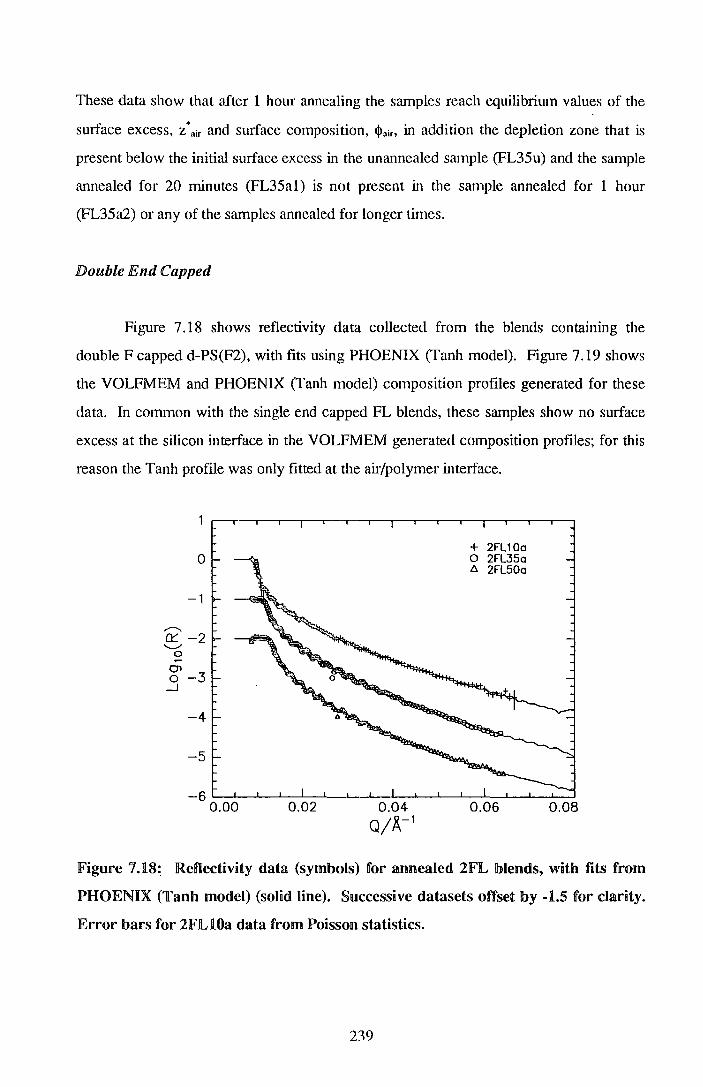
These data show that after 1 hour annealing the samples reach equilibrium values of the
surface excess, z*air and smface composition, G>au-, in addition the depletion zone that is
present below the initial surface excess in the unannealed sample (FL35u) and the sample
annealed for 20 minutes (FL35al) is not present in the sample annealed for 1 hour
(FL35a2) or any of the samples annealed for longer times.
Double End Capped
Figure 7.18 shows reflectivity data collected from the blends containing the
double F capped d-PS(F2), with fits using PHOENIX (fanh model). Figure 7.19 shows
the VOLFMEM and PHOENIX (fanh model) composition profiles generated for these
data. In common with the single end capped FL blends, these samples show no surface
excess at the silicon interface in the VOLFMEM generated composition profiles; for this
reason the Tanh profile was only fitted at the air/polymer interface.
0
-1
0'1 0 -3 _J
-4
-5
0.02 0.04 o;.z.-1
+ 2FL10a o 2FL35a t:. 2FL50a
0.06 0.08
!Figure 7.18: Reflectivity data (symbols) for annealledl 2FlL blends, with fits from
PHOENIX (Tanh model) (solid Dine). Successive datasets offset by -1.5 for clarity.
Error bars for 2FlL10a data from Poisson statistics.
239
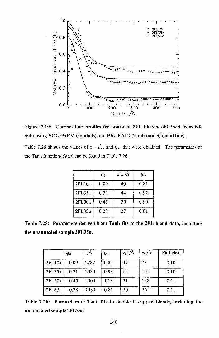
............ lJ..._
(;) 0.8 Q_
I u
c 0
....... 0 0 .t: 0.4
Q)
E :::J 0 0.2 >
100
0 2Fl10a l:l. 2Fl.35a + 2FL50a
oa00000ooooo0000oooooooooooooooooo
200 300 400 500
Depth /A
lFngure 7.19: Compositnon pmfiDes for anneaned 2JFL blel!lldls, obtained fmm NJR
data using VOLJFMEM (symlbolls) al!lld !PHOENIX (Tanh modlel) (solidi nine).
Table 7.25 shows the values of <J>s, z *.,ir and <Pair that were obtained. The parameters of
the Tanh functions fitted can be found in Table 7.26.
<Ps z*air/A ~air
2FL10a 0.09 40 0.81
2FL35a 0.31 44 0.92
2FL50a 0.45 39 0.99
2FL35u 0.28 27 0.81
Table 7.25: Parameters derived from Tanh fits to the 2FL blend data, including
the unannealed sample 2FL35u.
0 0
w/A Fit Index <Ps 1/A <!>I Zorr/A
2FL10a 0.09 2787 0.89 49 78 0.10
2FL35a 0.31 2380 0.98 65 101 0.10
2FL50a 0.45 2000 1.13 51 138 0.11
2FL35u 0.28 2380 0.81 50 36 0.11
Table 7.26: Parameters of Tanh fits to double F capped blends, including the
ummnealed samplle 2FL35u.
240

Only one unannealed sample was run (2FL35u), multilayer fits were carried out on this
blend and the values of z *air, z • der, <Pair, <Pdep and <Ps obtained can be found in Table 7.27,
the parameters of the multilayer fit can be found in Table 7 .28.
<Pair z*air!A <J>dep z*dep/A <Ps
2FL35u 0.89 32 0.22 6 0.29
1I'albHe 7.27: Parameters dlerivedl from a mQJilltnlayer fnt to tlhe 21FIL35Ull dlata.
<j>l zdA CJ1/A <1>2 zdA cr2/A <1>3 Z3/A Fit Index
2FL35u 0.89 48 30 0.22 95 40 0.46 2679 0.10
1I'albHe 7.28: lFit !Parameters of mllllBtinayer model for ttlh.e 2lFIL35Ull data.
241

7.3 Discussion
It has been shown4 that smface enrichment occurs in high molecular weight
blends of d-PS/h-PS, driven by a surface energy difference of, l'ly = 0.078 mJ m-2,
between the hydrogenous and deuterated polymers. The theory of Schmidt and Binder5
gives a good description of the surface enrichment behaviour observed such in high
molecular weight polymers blends. Using this theory it can be shown that virtually no
surface enrichment is expected in the low molecular weight d-PS(F)/h-PS (FL) blends
studied here. This prediction has been confinned by workers at the University of
Strathclyde1 using Secondary Ion Mass Spectrometry (SIMS), the absence of surface
enriclunent in the low molecular weight d-PS/h-PS arises because the phase boundary in
the low molecular weight system is at a much lower temperature than in the high
molecular weight blend and surface enrichment is strongly enhanced close to the phase
boundary. Therefore the substantial surface excesses observed in the low molecular
weight d-PS(F)/h-PS must be caused by the perfluorohexane end group end attaching the
d-PS(F) to the air interface, fonning a brush. The self consistent field (SCF) theory of
polymer brushes in polymer matrices, developed by Shull6, was outlined in section 2.3.1.
The predictions of this theory will be compared to the results described above.
In order to compare the results of theoretical calculations made using relatively
small 'polymers' with the experimental results, a number of procedures will be adopted
to normalise the results of both theory and experiment. Firstly the normalised surface
excess z*/Rg will be used, where Rg is the radius of gyration of the d-PS(F), this will also
facilitate comparisons between high and low molecular weight blends. The radii of
gyration of the d-PS(F) used in this work are 46A and 212A for the FL and FH blends,
respectively. These values are calculated from the molecular weights of the polymers
measured by size exclusion chromatography and literature values of <SJMw'h>7 • These
radii of gyration will also be used to normalise the depth into the sample nonnal to the
surface, z/Rg. Values of the Flory- Huggins interaction parameter, x. used in the model
were fixed such that the value of xN was equal to the value of xN calculated for the
experimental system, where N is the geometric mean of the degrees of polymerisation.
This ensures that the model system is the same 'distance' from the phase boundary as the
experimental system, for the low molecular blend xN is effectively zero ( and so X was
set to zero for these models). The degrees of polymerisation of the two components in
242

the Shull model were set to 160 and 100 for the non-adsorbing (= h-PS) and absorbing
(= d-PS(F)) polymers. This preserves the ratio NHINo = 1.6, found in the low molecular
weight blends. Finally the surface free energy difference, p, defined below, is used.
JE.qpu a 1i on 7 .4l
where Xeb is the energy of interaction between the perfluorohexane end group and the
bulk blend and Xes is the difference in surface energy between the end group and the bulk.
Model calculations were made with values of the bulk volume fraction of d-PS(F), <(>B,
fixed at the values detennined experimentally using PHOENIX (Tanh model). The only
variable that is available to fit is (Xe b- Xes), the model is only sensitive to the combination
of Xeb and XeS. not separately. The aim of this modelling was to fit the fonn of the
composition profile, <(>(z/Rg). the quality of this fit can be evaluated by comparing z */Rg
vs <!>Band ($air- $B) vs <I>B· The fit of predicted values of z*/Rg to experimental val\}es of
z*/Rg will be the principal criterion because z*/Rg is less susceptible to experimental error
than ($air - $B). The nature of the SCF theory calculations means it is not possible to
perform an automatic least squares fit of the theoretical prediction to the experimental
data. So the best fit value of (Xe b- Xe5) was obtained by eye, this value corresponds to p
= 1.9. The fitted value of (Xeb- x/) is for a system where No= 100, in the experimental
system Nn = 274, putting this value and P = 1.9 into Equation 7.4 we find that (Xeb- Xes)
= 4.0 in the experimental system. Figure 7.20 shows a comparison of selected
experimental <(>(z/Rg) profiles with theoretically predicted <(>(z/Rg). To obtain units of
z/Rg in the lattice model, z in lattice units is divided by 4.082 (this is because Rg =
a>J(No/6), and a = 1 for the model and ..J(No/6) = 4.082 for N0 = 100). Figure 7.21
shows the theoretical calculations for z*/Rg vs <(>s, with P = 1.9, compared to the
experimental values. The broken lines are the theoretical values calculated using p = 1. 7
and P = 2.1. Similarly Figure 7.22 is a comparison of the ($air - <(> 8 ) vs <(> 8 values. These
fits were all done using the values of <!>B obtained from the PHOENIX (Tanh model) fits,
if the nominal values were used then a slightly lower value of P would be obtained.
243
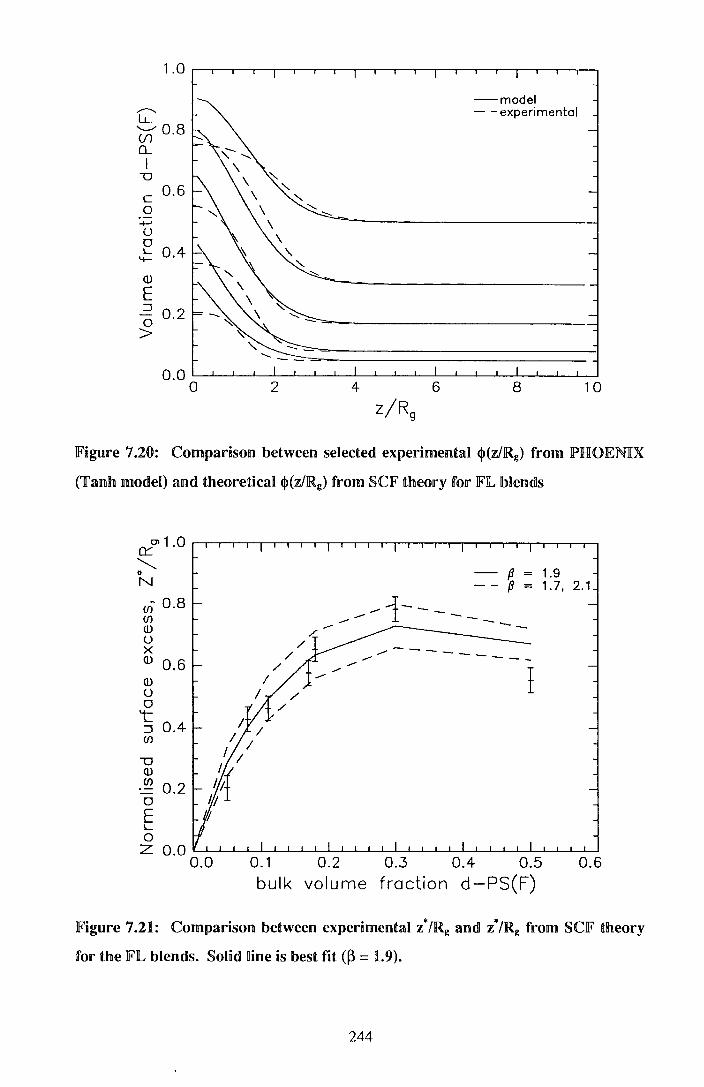
1.0
-model ,..---.._ - -experimental LL (;)0.8 Q_
I -o c 0.6 0
-1-' u 0
0.4 L 4--
Q)
E ::l 0.2 -0 >
0.0 0 2 4 6 8 10
z/R9
Figure 7.20: Compar!son between selected experimental cp(z/lRg) lfrom lP'JH!OlEMX
(1I'anllln moden) anun theoreticaH cp(z/Rg) from SCF theory for JFIL lblemns
n:::O'I 1 . 0 ~
~ 1.9 * N 1.7, 2.1 u) 0.8 -i---(f) - --- --Q) -- -u X ---- ---Q) 0.6 - ----- I Q)
u / 0 / 4--L
0.4 I ::l I (f) I I
-o I I Q) ~~± (f)
0.2 0 /,'f
E If L
0 z 0.0
0.0 0.1 0.2 0.3 0.4 0.5 0.6 bulk volume fraction d-PS(F)
Figure 7.21: Comparison between expedmental z*/Rg andl z"/Rg from SCF theory
for the FIL blends. Solid Dine is best fit (~ = 11.9).
244

,..--.... CD
-e-
0.5
0.4
1._ 0.3 ·c;
-& ......._,
0.2
0.1
-----........ - (3 // ................ --(3
........ --L...___ ....................
-- I ...._ ........... /,.-- ------ .......... --
1.9 1.7, 2.1
..._ --
I
0.1 0.2 0.3 0.4 0.5 0.6 bulk volume fraction d-PS(F)
lFngure 7.22: Comparison !between experimental (lj>alr - lj>8) and theoretical
prednction from SCF theory. SoiRd Bine ns fmm best fit to z*/Rg (j3 = li.9).
The fit to z*/Rg vs cJ>B is good, the only significant deviation from the theory is for the
blend with cJ>B = 0.50, however Figure 7.22 shows that the theory systematically over
estimates the surface volume fraction, «<>air. this is also apparent in the composition
profiles shown in Figure 7.20. Such deviations have been observed8 between theoretical
predictions based on mean field theories and the surface enrichment in high molecular
weight d-PS/h-PS and can be explained by assuming that the surface attraction is not
limited solely to the first layer of segments at the surface.
In principle it should be possible to estimate j3 using data in the literature and the
measured value of N0 for the low molecular weight d-PS(F) . Xeb is the interaction
parameter of perfluorohexane I styrene for a single lattice cell, in units of kB T. This can
be estimated from the solubility parameters of polystyrene, Ors, and poly
(tetrafluoroethylene), ~. making the assumption that the perfluorohexane can be
treated as a short piece of PTFE. Xeb is calculated as follows 9:
245
lEqa.natnoll11 7.5
Where VL is the volume of a lattice cell, in Shull's program VL = a3, where a is the
statistical segment length, for polystyrene a= 6.7 A, hence VL = 3.01xl0-22 cm3• Values
of brs and brTFE can be found in reference 7, they are Ors = 20.2 J cm-3 and 8rTFE = 12.7 J
cm-3• Using Equation 7.5 (T = 400K) this gives a value of Xeb = 3.1. Xes is the surface
energy difference per lattice cell, again in units of kB T. Values for the surface energies of
polystyrene and a short chain perfluorinated hydrocarbon (C21F44) can be also be found in
reference 7, these values are 32.8 rnJ m-2 and 14.4 mJ m-2 for PS and C21F44, respectively
- interpolated to 400K. The difference in surface energies, ,'),:y = 18.4 mJ m-2• This
corresponds to a value of x/ = -1.50, calculated using Equation 7 .6, below:
1Equatnoll11 7.6
where nL is the number of lattice cells per metre square, the area of one lattice cell= a2 =
45A2• Positive values of ~ favour brush formation, hence the sign of Xes is negative
because it occurs as -xe" in Equation 7.4. The value of (Xeb -Xes) calculated using these
estimated values is 4.6 which compares with a value of 4.0 which is obtained
experimentally, i.e. by using data readily available in the literature a good estimate of the
~ parameter and hence the brush fonnation behaviour of this blend could be obtained.
The scaling theory, outlined in section 2.3.2, can be used to gain a physical
insight into the behaviour of the d-PS(F) polymers which are end attached at the air
surface. The parameter of interest is the dimensionless grafting density, cr, defined as the
product of the area occupied by one segment, b2, multiplied by the number of end
attached chains per unit area, for polystyrene b = 5.5A. It can be shown that a is given
by:
246

lEqUJation 7. 7
This gives values of cr in the range 0.006 - 0.022 for the low molecular weight FL blends,
the average distance between graft points, Do, can be calculated from:
lEquatiollll 7.8
For this system Do ranges from 37 A to 71 A. These values of cr lie above the limit cr =
No-615 (=0.0012) which is where chains change from being independent 'mushrooms' to
overlapping brushes, but the values are below the limit cr = NHNo-312 (= 0.095) where the
brush becomes strongly stretched. In this case the chains are in the 'screened brush'
regime where the end attached chains are only weakly stretched and the brush is still
penetrated by the h-PS matrix chains. Scaling theory will fail to predict the form of the
near surface composition profile, because for brush systems such as those studied here
where the matrix is a relatively high molecular weight (when compared to the solvent
molecules typically used in scaling theory) the loss in entropy that the matrix polymer
suffers on being confined to the surface is not accounted for so that scaling will predict a
maximum in the concentration of the end attached polymer at a finite distance from the
surface, with matrix polymers 'filling in' the near surface region to maintain constant
density. SCF theory accounts for this reduction in matrix entropy and shows a maximum
in the end attached polymer density at the surface which decreases monotonically into
the bulk.
Turning to the blends, containing d-PS(F2) where there are perfluorohexane end
caps at both ends of the deuterated polymer, for which N0 = 500 and Rg = 61A. Again
mean field calculations show that the amount of surface enriclunent occmTing in these
blends is negligible. SCF theory calculations can be used to predict the degree of brush
fonnation, in common with the single end capped low molecular weight blends X = 0 was
used in the model because the product xN is effectively zero for these blends. The ratio
Nw'No = 0.86 for the 2FL blends so the degrees of polymerisation for the non-adsorbing
(=h-PS) and absorbing (=d-PS(F2)) polymers were set to 86 and 100 respectively. The
247

results from the FL blends show that (Xeb- x/) = 4.0, insetting this value and N0 = 500
into Equation 7.4 a value of~ = 1.5 is obtained. This is the free energy of sticking for
each end of the d-PS(F2) polymer. Model profiles with (Xeb- xe') = 3.1 were generated
using SCF theory, this value conesponds to ~ = 1.5 in a model with N0 = 500. A
comparison of the model and experimentally detennined <J>(z/Rg) are shown in Figure
7 .23. Figure 7.24 shows a comparison of theoretical and experimental values of z •'!Rg vs
<l>n for the 2FL blends, similarly Figure 7.25 shows a comparison of ($air- <l>n) vs <J>8 •
1.0
r-.... N
-model - -experimental
~0.8 (j) Q_
I -o
0.6 c 0
-+-' u 0 0.4 L
'+-
Q)
E ::J 0.2 -0 >
0.0 0 2 4 6 8 10
Figure 7.23: Comparison of experimental cjl(z/Rg) from PHOENIX (Tanh model)
and theoretical cjl(z/Rg) from SCF theory model for 2FL blends.
It is apparent that, with the parameters extracted from the single end capped FL blends
an accurate prediction of the z*/Rg vs cjl8 behaviour in the 2FL blends can be obtained.
However, in contrast to FL blends, the SCF theory under estimates (rather than over
estimates) the values of ($air - <l>s) that are observed in the experimental system.
Examining Figure 7.23 it can be seen that this corresponds to the experimental system
exhibiting near surface composition profiles that are 'taller' and 'thinner' than the
modelled profiles.
248

cr: (Jl 1 . 0 ,-.----,-.,....,---,--.--.--r--r-.-.--.-...,...,-,---.--.--r--r-.-.--.-,...--,-,--..-,..,..--,----,
"--.. " N
(I)~ 0.8 (I) Q)
0 X Q) 0.6 Q) 0 0 4-L ::J 0.4 (I)
-o Q) (I)
0.2 0
E L 0 z 0.0
0.0
_ ....... __ {3 {3
1.5 1..3, 1.7
0.1 0.2 0.3 0.4 0.5 0.6 bulk volume fraction d-PS(F2)
Figure 7.24: Comparison of experimental z•/Rg and z•/Rg from SCF theory model
for the 2FL blends. Solid line is fit using the value of (Xeh- Xe5) from the FL blends
equivalent to p = 1.5.
I ~ = 1.5 1.3, 1.7
0.6 --- ------l
,.......... Q)
-e-1._ 0.4
0
-a-'-../
0.2
o.o~~~~~~~~~~~~~~~~~~~~~
0.0 0.1 0.2 0.3 0.4 0.5 bulk volume fraction d-PS(F2)
0.6
Figure 7.25: Comparison between experimental C<Pair - <jl8 ) and theoretical
prediction from SCF theory model. Solid line is from best fit to z•/Rg for the FL
blends equivalent to P = 1.5.
249

Further calculations with the SCF themy show that this difference is not driven by the
tiny difference in surface energies (= 0.006k8 T) between d-PS and h-PS segments, i.e.
this is not opportunistic surface enrichment arising in chains that have been brought close
to the smface by being attached at both ends. An insight into this behaviour can be
obtained by examining the grafting densities, cr, for these blends. For the 2FL blends
each polymer absorbed at the air surface represents up to two graft points. Therefore:
2z* cr:::;;
Nb
Equation 7.9
The values of cr calculated for these blends lie between 0.028 and 0.030, which is in the
same 'screened brush' regime as the single end capped FL blends. The limits of this
regime are at N0 -615 (=0.0006) and N1-1N0 -
312 (= 0.038), so the 2FL blends lie rather closer
to the stretched brush limit than the FL blends. Calculating the average separation of
graft points, Da, we find values >32A. This is substantially less than the root mean
square end to end distance(= Rg..J6) for the d-PS(F2) polymer, which is 115A. It may be
that the initial distribution of end groups in the plane of the air - polymer interface is not
at equilibrium and that over a period of time the surface volume fraction of d-PS(F2) will
relax to the expected value, however one would expect the relaxation to occur relatively
rapidly since the attachment energy of the end group to the surface is quite small.
The high molecular weight d-PS(F)/h-PS blends exhibited surface excesses at
both the air and silicon interfaces, the 'normal' high molecular weight d-PS/h-PS blends
also exhibited smface excesses at both interfaces. On the whole surface emiclunent has
not been observed at the polymer-substrate interface for d-PS/h-PS blends, the difference
with this work would appear to be because this work was done using silicon with it's
native silicon dioxide layer intact. This conclusion is supported by the work of Frantz et
a/10 on the competitive absorption of d-PS and h-PS, from cyclohexane solution onto a
silicon attenuated total reflection (A TR) ctystal with a silicon oxide layer and the work
of Budkowski et a/11 on d-PS/h-PS blends on silicon with an intact oxide layer.
The results from the NRA measurements on the 'nonnal' d-PS/h-PS blends show
an excess at the silicon inteiface around half that observed at the air intetface, this
suggests that the difference in surface energy between ci-PS and h-PS versus silicon
250

oxide is -0.04 mJ m-2, this is at the low end of the wide range of values that Frantz eta/
have observed but is larger than the value obtained by Budkowski eta/. This difference
is smaller than the difference of 0.078 mJ m-2 that is observed between d-PS and h-PS at
the air interface.
In principle it should be possible to predict the parameters, z */Rg and (<!>au- - <j> 8 ), of
the near surface composition profiles observed in the high molecular weight blends by
adding together the contributions from surface enrichment and brush fonnation.
Calculations of the expected surface enrichment behaviour were done using the Jones
and Kramer12 simplifications to the mean field themy of Schmidt and Binder. The values
of the parameters used were: f):y = 0.078 mJ m-2, X = 1.77x10⁴ (from Bates and
Wignall13) and the degree of polymerisation, N = 9800. The calculations were done
assuming a symmetric blend with NH = No and the value of N used here is the geometric
mean of the values NH and No of the polymers used, this is the scheme suggested for
asymmetric blends in reference 12. These calculations produce values for the surface
excess that are significantly larger than the measured values, where it is suspected that
both surface enrichment and brush formation are taking place. One explanation for this
could be that the blends have had insufficient annealing time to reach equilibrium,
although this is unlikely because SIMS data on these polymers has shown that an
equilibrium in the surface volume fraction of d-PS(F) has been reached. Putting aside
this possibility a further attempt to calculate the expected surface excess from theory was
made, collaborators at the University of Strathclyde have found, using SIMS, that the
surface volume fraction of d-PS in a d-PS/h-PS blend with similar molecular weights to
those used here is 0.45 for a blend with <j> 8 = 0.15. The molecular weights of the blend
components were 816,000 and 1,710,00 for the d-PS and h-PS respectively. Using the
parameters 11y = 0.078 mJ m-2, and N = 10950 (the geometric mean of the degrees of
polymerisation), the value of X was adjusted until the theoretical prediction of the surface
volume fraction matched the experimentally measured value. This was found to occur
when X = 0.58xl04. This value of X was then used to calculate the nonnalised surface
excess and the smface volume fractions expected in the high molecular weight FH
blends. The justification for this modification of the X value is that the asymmetry (i.e.
NH * No) in the blend changes the value of X from the value measured for symmetric
high molecular blends of d-PS/h-PS. Such a change in the X value has been shown in this
work for the d-PMMA/h-PMMA blend. This change in X will change the position of the
251

blend on the phase diagram in relative to the phase boundary and hence change the
surface enrichment behaviour. Moving on to the brush fonnation predictions: the value
of~ calculated for these blends, using Equation 7.4, is 0.16. The ratio of NHIN0 is 2.8
and to maintain this ratio values of NH = 140 and N0 = 50 were used in the model
calculations, this means that value of (Xeb- Xes) required in the model is 1.3. The value of
X used was 0.007, corresponding to a value of xN = 0.64, where N is the geometric
mean of NH and N0 , this is equal to the value of xN used in the surface enrichment
calculations. Figure 7.26 shows the experimental values of z */Rg vs <l>s and the values of
z*/Rg obtained from the theoretical calculations of both brush formation and surface
enrichment- the sum of these contributions is also included. Similarly Figure 7.27 shows
the experimental behaviour and the theoretical predictions for (<!>air - <l>s) vs <l>s-
0>0.6 0:::::
---........ .. N
0.5 (/) (/) Q)
0 0.4 X
Q)
Q) 0
0.3 0 '+-L. :J (/)
0.2 -o Q) (/)
/' /'
-·-·-·-·-·/·~·-·-
/ /
/
/' /'
/
I
0 0.1 / / + Experimental E / -Brush + Enrichment L. / - -Brush (theory) 0 / / -·-Enrichment ttheory) ~ 0.0 ~/~~~~~--~~~~~~~--~~~~~~--~
0.0 0.1 0.2 0.3 0.4
Bulk volume fraction d-PS(F)
Figure 7.26: Comparison between experimental z*/Rg and theoretical predictions
from the combination of SCF theory models (brush) and mean field theory
(enrichment).
252

.........--. m
-e-
0.5 .
0.4
1.._ 0.3 0
-e-..........,.
0.2
0.1
,-" /
-·-·-·-. ·-·-·-·
--------_.... _.... + Experimental
_.... _.... -Brush + Enrichment _.... _.... - -Brush (theory)
_.... -·-Enrichment ttheory) 0.0 ~/~~-L~~--L-~~_L~~L-L-~-L-L~--L-~~~
0.0 0.1 0.2 0.3 0.4
Bulk volume fraction d-PS(F)
Figure 7.27: Comparison between experimental («JlaJr - ljl8) and theoretical
predictions from the combination of SCIF' theory models (brush) and mean fneld
theory (enrichment).
The fit of the combined surface enrichment plus brush fonnation to z*/Rg vs «JlB is very
good and in common with the low molecular weight FL blends («Pair - «JlB) is slightly over
estimated by the theory. Clearly the use of the modified X parameter makes this result a
little less conclusive, but nevertheless it appears that using a single parameter extracted
from the low molecular weight FL blends, (Xeb- Xe'), it is possible to predict the brush
fonnation behaviour in the FL blends, the double F capped 2FL blends and the high
molecular weight FH blends.
The final area to cover in this discussion is the non-equilibrium and approach to
equilibrium behaviour of these blends. Unannealed films of all the blends exhibit some
sort of non-unifonn structure. For the FL5 and FH5 blends, structure is essentially
unchanged by annealing. The structures in the unannealed FH blends, as revealed by the
VOLFMEM fits, are not consistent across the range of bulk compositions, «JlB, i.e. the
FH25u and FH50u blends exhibit depletion of d-PS(F) from the surface whilst the FH5u
and FH35u blends exhibit a surface excess of the d-PS(F). The behaviour in the FL
blends, both for varying «JlB and varying casting solution concentration, is more unifonn.
This is despite the fact that these samples were prepared on three separate occasions, as
253

opposed to the single occasion on which the FH blends were prepared. This suggest that
the FH blends are more sensitive to the casting conditions than the FL blends. The same
procedure was used to cast films of all the blends: a large aliquot of the casting solution
was placed onto the silicon substrate and then the substrate was spun for 60 seconds.
However the details of this process are not precisely controlled, i.e. the exact amount of
solution, the time between placing the solution on the substrate and starting the spinner,
the temperature, the amount of solvent vapour in the immediate vicinity of the forming
film, all of these factors could influence the structures observed in the unannealed film.
To probe the influence of these factors experiments need to be repeated to establish the
degree of variability in unannealed cast in a nominally identical manner. Since the FL
blends seem less sensitive to these effects the remainder of this discussion will
concentrate on the FL blends.
The three layer models used to fit the composition profiles in the unannealed
films indicate a depletion layer below the initial srnface excess, but the size of this
depletion, z • der, is considerably smaller than the corresponding surface excess. This
implies that the model is not accurately describing the composition profile in the sample,
because if it were then the conservation of mass would force z"air = z"dep, the reason for
this discrepancy probably lies in the relative insensitivity of NR to structures that vary
slowly over a long length scale. The measured z*dep is more an indication of how
localised the depletion is to the surface than an accurate measure of the 'true' z * dep·
Figure 7.28 shows the variation of z *air as a function of cJ>B, for both unannealed
and annealed FL blends, the measured z*dep is also included. The surface excess in the
unannealed blends has the same behaviour with <l>n as the surface excess in the annealed
film, but with values of a lower magnitude. The measured z * dep shows a small increase
across the composition range. All these values were calculated from the PHOENIX
(multilayer model) fits for consistency. Figure 7.29 shows the variation of z*air and z*dep
as a function of casting solution concentration for the series of blends A35u, B35u, C35u
and D35u. There is a small decrease in the surface excess as the casting solution
concentration is decreased accompanied by a small increase in the measured z*dep. the
decrease is largest between the blends cast from 0.05 and 0.025 weight fraction polymer
solutions.
There are two stages to the process by which the srnface excess develops in the
unannealed films:
254

(1) The equilibrium structure in the casting solution as it lies on the substrate. It has
been observed that in polystyrene I toluene solutions 14 that there is a region at the
surface of the solution that is depleted in polystyrene. This is driven by two forces, the
toluene has a lower smface energy than the polystyrene and it also loses less entropy on
being confined to the surface than the polystyrene.
(2) After the spinning process starts the solvent will evaporate until a point is reached
where the polymer is the dominant species at the surface.
liN
L
0
-~ 20 0
en en Q) 10 u X
w
0 annealed z•air 6. unannealed z• air + unannealed z•dep
0.1 0.2 0.3 0.4 0.5 Bulk volume fraction d-PS(F)
0.6
Figure 7.28: The surface excess z .. a1r for both unanrnealedl and annealed FlL !blends,
along with measured z*dep· Calculated from PHOENIX (multilayer fits).
255

25
0 .
z.air 0<( 1'1. Z dep
"-..20 ,..--.... 0.. Ql
"U
* N
L 15 0
.!:::: 0
* ~ 10
(/)
I (/) Q)
u 5 I X
I I w
0 ~~~~-L~J-~L-~~~~-L~J-~~~~~~ 0.00 0.02 0.04 0.06 0.08 0.10 0.12
Weight fraction polymer
lFigure 7.29: The surface excess z*alr and measured z*dep for the sernes of FIL lblends
cast fmm so!utions of different concentration.
The blend will still be mobile, plasticised by the presence of the toluene and the polymer
in the film will start to move towards the solid state equilibrium structure. This process
will be arrested when still more solvent has left the film and the Tg of the blend rises
above the casting temperature. The time which this second stage lasts will depend on the
thickness of the final film, a thin film will lose a larger proportion of solvent than a
similar thicker film and so structure will be frozen into a thin film more rapidly.
These two processes are linked in this experiment because the casting solution
concentration, which will have some influence on the equilibrium structure in the casting
solution, also controls the film thickness and hence the time it takes for structure to
freeze into the flhn. Surface tension measurements carried out by Wills15 show that the
surface tension of a solution of the pure low molecular weight d-PS(F) polymer was very
slightly lower than that of pure toluene, suggesting that there is some excess of the
fluorinated end group at the smface of the polymer solution. However there was no
measurable change in the surface tension as a function of the solution concentration over
the range 2.5% w/w to 10% w/w d-PS(F). Given the very small size of the effect it
would be difficult to draw any fmther conclusions from these data.
256

An estimate of the self diffusion coefficient, D,, for the low molecular weight d
PS(F) in h-PS can be made from the surface excesses obtained in experiment (5), where
blends containing 0.35 bulk volume fraction d-PS(F) were annealed for periods of up to
2 days. Figure 7.30 shows the development of the surface excess as a function of
"-'(annealing time, t), the equilibrium surface excess is reached after only one hour
annealing at 403K. The diffusion coefficient can be obtained from these data using a
modified version of the scheme used by Jones and Kramer16• The conservation of mass
dictates that:
Equation 7.10
where z*0 is the surface excess in the unannealed blend, z*o + z*(t) is the smface excess at
time t, <j>d(t) is the volume fraction of d-PS(F) in the depletion zone immediately below
the surface excess, in this analysis it is assumed that the smface excess is always in
equilibrium with this value.
ex( ~40 r-
L
·c; * N
(fJ 30 -(fJ Q) u X Q)
Q) ()
0 '+L
20 -
::::J 10 -(f)
I -
-
I -
I -
Figure 7.30: Development of the surface excess in FL35 as a function of annealing
time. Values are from PHOENIX (Tanh model).
257

(Dst) 112 is the diffusion length and it is assumed that the size of the depletion layer is of
order (D,t) 112• For the d-PS/h-PS system studied by Jones and Kramer it was found that
z*eq = K <!>B, where z*eq is the equilibrium value of the surface excess for bulk volume
fraction d-PS, <)>B, K is a constant. This means that z\t)=K <j>d(t) for d-PS/h-PS. In this
system the relationship between z • and <!>B is better described by:
Equation 7.U
where A and B are constants. Using this expression would complicate the analysis
considerably and so the approximation z*eq = K <!>B will be used. Substituting for <)>d(t) in
Equation 7.10 we find:
Equation 7.12
The characteristic time tc is defined as the time when the smiace excess has reached a
value half way between z*0 and z*eq· Substituting this into Equation 7.12 and re
arranging:
Equation 7.13
For the FL blend used z*eq = 36A, z*o = 17A, <)>B = 0.30 and the halfway point at z* = 27A
is reached after around 30 minutes, hence D.""" 3xl0-15cm2s·1• Wool and Whitlow17 have
measured the diffusion coefficient of d-PS in h-PS for approximately symmetric blends
with molecular weights > 100,000 over a range of temperatures spanning the annealing
temperature used here. Extrapolating these values to the molecular weights used here
using the relationship Ds oc Mw-2 a value for the diffusion coefficient of -lx10-15 cm2 s·1 is
obtained. Given the numerous approximations in this analysis used here and the paucity
of data available between the unannealed and equilibrium state this value is in agreement
with the value calculated here.
258

7.4 Conclusions
The smface composition profiles in a series of d-PS(F)/h-PS blends where the d
PS has been end functionalized with perfluorohexane were detennined using NRA and
NR. It was found that a SCF theory of polymer brushes could accurately describe the
behaviour in low molecular weight single end capped (FL) blends, low molecular weight
double end capped (2FL) blends and high molecular weight single end capped (FH)
blends. The enthalpic interaction driving the brush fonnation, (Xeb- Xe5), was fitted with
a value of 4.0, using the data from the FL blend. Using this value for the enthalpic
interaction and no other free parameters it was possible to obtain good predictions of the
behaviour in the 2FL and FH blends. It was found that the SCF theory over estimated
the value of (~air - ~B) for the FL and FH blends but under estimated (~air - ~B) for the
2FL blends, a possible explanation for this is that the end groups in the 2FL blends not
reaching their equilibrium distribution in the plane of the air intetface. An estimate of
(Xeb - Xe5) = 4.6 was obtained from literature values of surface energy and solubility
parameters, this value is close to the experimentally detennined value. It should be noted
that the value of (Xeb- xe') = 4.0 is likely be the largest that can be obtained for a small
end group at the air interrace. Crude calculations show that for the FL blends the
perfluorohexane end groups produce a surface excess that is equivalent to that produced
by a smface energy difference -0.5 mJ m·2, which is small when compared to the
differences in smface energy generally observed between different polymers.
A diffusion coefficient, D,"" 3xl0-15 cm2 s·1 was obtained for the d-PS(F) in the
FL blends, this value of Ds is in broad agreement with values in the literature. It was
found that the FL blends reached an equilibrium value for the surtace excess after around
one hour annealing at 403K.
259

7.5 !References for Secfion 7
1. S. Affrossman, M. Hartshorne, T. Kiff, R.A. Pethrick, R.W. Richards,
Macromolecules, 27(6), 1994, 1588.
2. G. Reiter, Langmuir, 9(5), 1993, 1344.
3. W.H. Press, S.A. Teukolsky, W.T. Vetterling, B.P. Flannery, 'Numerical Recipes in
FORTRAN 2"d ed. ', Cambridge University Press, 1992.
4 . R.A.L. Jones, E.J. Kramer, M.H. Rafailovich, J. Sokolov, S.A. Scharwz, Physical
Review Letters, 62(3), 1989, 280.
5. I. Schmidt, K. Binder, Journal de Physique, 46, 1985, 1631.
6. K.R. Shull, Journal of Chemical Physics, 94(8), 1991, 5723.
7. J. Brandrup, E. H. Immergut, 'Polymer Handbook 3rd ed. pp VII/36', J.Wiley &
Sons, 1989.
8. R.A.L. Jones, L.J. Norton, E.J. Kramer, R.J. Composto, R.S. Stein, T.P. Russell, A.
Mansour, A. Karim, G.P. Fekher, M.H. Rafailovich, J. Sokolov, X. Zhao, S.A. Schwarz,
Europhysics Letters, 12(1), 1990, 41.
9. F.S. Bates, G.D. Wignall, Macromolecules, 19, 1986, 932.
10. P. Frantz, D.C. Dagmar, S. Granick, Macromolecules, 24, 1991, 1868.
11 . A. Budkowski, U. Steiner, J. Klein, Journal of Chemical Physics, 97(7), 1992,
5229.
12. (a) R.A.L. Jones, E.J. Kramer, Polymer, 34(1), 1993, 115. (b) R.A.L. Jones,
Polymer, 35(10), 1994, 2160.
13. F.S. Bates, G.D. Wignall, Macromolecules, 19. 1986, 932.
14. L.T. Lee, 0. Guiselin, A. Lapp, B.Farnoux, J. Penfold, Physical Review Letters,
67(20), 1991, 2838.
15 . S. Wills, unpublished results.
16. R.A.L. Jones, E.J. Kramer, Philosophical Magazine B, 62(2), 1990, 129.
17. S.J. Whitlow, R.P. Wool, Macromolecules, 24, 1991, 5926.
260

This page left intentionally blank
261
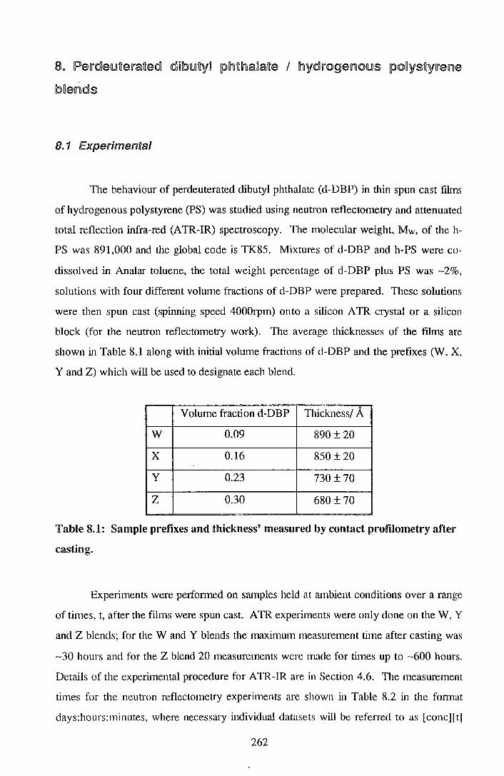
8. IPe~rde!!.ntera~ftedl <dlilb!!.nity~ p~ftlrila~~afte I hyd~rogelnl(Q)ll..nS po~ystyre111e
lb~e~n~ds
8. 1 Experimen'ial
The behaviour of perdeuterated dibutyl phthalate (d-DBP) in thin spun cast films
of hydrogenous polystyrene (PS) was studied using neutron reflectometry and attenuated
total reflection infra-red (ATR-IR) spectroscopy. The molecular weight, Mw, of the h
PS was 891,000 and the global code is TK85. Mixtures of d-DBP and h-PS were co
dissolved in Analar toluene, the total weight percentage of d-DBP plus PS was -2%,
solutions with four different volume fractions of d-DBP were prepared. These solutions
were then spun cast (spinning speed 4000rpm) onto a silicon ATR crystal or a silicon
block (for the neutron reflectometry work). The average thicknesses of the films are
shown in Table 8.1 along with initial volume fractions of d-DBP and the prefixes (yv, X,
Y and Z) which will be used to designate each blend.
Volume fraction d-DBP Thickness/ A w 0.09 890 ± 20
X 0.16 850 ± 20
y 0.23 730 ± 70
z 0.30 680 ± 70
Table 8.1: Sample prefixes and thickness' measured by contact profilometry after
casting.
Experiments were performed on samples held at ambient conditions over a range
of times, t, after the films were spun cast. ATR experiments were only done on theW, Y
and Z blends; for the W and Y blends the maximum measurement time after casting was
-30 hours and for the Z blend 20 measurements were made for times up to -600 hours.
Details of the experimental procedure for ATR-IR are in Section 4.6. The measurement
times for the neutron reflectometry experiments are shown in Table 8.2 in the fonnat
days:hours:minutes, where necessary individual datasets will be referred to as [conc][t]
262
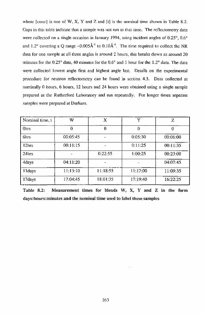
where [cone] is one of W, X, Y and Z and [t] is the nominal time shown in Table 8.2.
Gaps in this table indicate that a sample was not run at that time. The reflectometry data
were collected on a single occasion in January 1994, using incident angles of 0.25°, 0.6°
and 1.2° coveting a Q range -0.005A-1 to O.lOA-1• The time required to collect the NR
data for one sample at all three angles is around 2 hours, this breaks down as around 20
minutes for the 0.25° data, 40 minutes for the 0.6° and 1 hour for the 1.2° data. The data
were collected lowest angle first and highest angle last. Details on the experimental
procedure for neutron reflectometry can be found in section 4.3. Data collected at
nominally 0 hours, 6 hours, 12 hours and 24 hours were obtained using a single sample
prepared at the Rutherford Laboratory and run repeatedly. For longer times separate
samples were prepared at Durham.
Nominal time, t w X y z Ohrs 0 0 0 0
6hrs 00:05:45 - 0:05:30 00:06:00
12hrs 00:11:15 - 0:11:25 00:11:35
24hrs - 0:22:55 1:00:25 00:23:00
4days 04:11:20 - - 04:07:45
11days 11:13:10 11:18:55 11:17:00 11:09:35
17days 17:04:45 18:01:35 17:19:40 16:22:25
TabBe 8.2: Measurement times for blends W, X, Y and Z in the form
dlays:hours:minutes and the 1111ominaD time used to label these sampBes
263

8.2 !Resulis
Figure 8.1 shows representative ATR-IR spectra from the Z blends. the
contribution from the silicon and other background contributions have been subtracted.
Spectra are the average of 64 scans. The atmospheric C02 band has been over
subtracted and this is the origin of the 'negative band' at -2350 cm-1• The series of
peaks between 3200 cm-1 and 2800 cm-1 are the C-H stretches of polystyrene. The
deuteration results in the equivalent C-D stretches in d-DBP being shifted to the 2000-
2300 cm-1 region of the spectrum. The strong peak at 1725 cm-1 is the carbonyl stretch,
which arises solely from the d-DBP.
0.18
<1)
g 0.16 0
..Q L 0 (/)
..Q
<t:: 0.14
0.12
-13 days - -8 hours - -0 hours
' tl ,, ,, 1,'11 I \ ~
-'# .. , ..... .,1,., ,, ..... ., ... ,, .. ., .. ,_ .. C-H
C=O
I, I
"' 0. 1 0 ..__......__,__.__.__.___.___.___.___.___.___.___....__..__.___.__.__--L---L---'---J
3500 3000 2500 2000 1500 Wavenumber /cm- 1
Figure 8.1: Selected ATR~IR spectra for the Z blend collected at the times
indicated, data offset for clarity.
The penetration depth, dp, at IR wavelength, A, for polystyrene on silicon is given
by:
A d = ----;::::::=====
P I 2 • 2 8 2 2rt-y fls; Slll atr - flps
Equation 8. L
264

where nsi = 3.4 is the refractive index of the silicon and nrs = 1.5 is the refractive index
of the polystyrene. eatr is the angle of incidence, which is 45° for all of these
experiments.. In this system the penetration depth falls in the range 1.0 ~-tm to 2.0 ~-tm for
the polystyrene C-H stretch and d-DBP carbonyl bands respectively. These values are
far larger than the film thickness and this means that the absorption peaks are insensitive
to the distribution of the d-DBP in the film but they are sensitive to the total amount of
d-DBP in the film. The amount of d-DBP in the film will be related to the area, Ac.x,
under either of d-DBP peaks (Ac.n or Ac=o) nonnalised by the area under the polystyrene
C-H stretch band, Ac.H· The areas under these peaks were measured using the peak area
function of the PE1600 spectrometer used to make these measurements. The limits of
the area integration were 3200-2800 cm·1 for the C-H stretch, 2285-2060cnf1 for the C
D stretch and 1670-1770 cm·1 for the carbonyl stretch. The limits of the baseline were
fixed at the same value as the integration limits, this is illustrated schematically in Figure
8.2
The average volume fraction of d-DBP in the films, ~av, is related linearly to the
ratios Ac.n/Ac-H and Ac=O/Ac-H, this is a result of the Beer - Lambert Law. To find the
constant of proportionality it was assumed that for the first measurements, made at less
than 10 minutes after casting, the amount of d-DBP in the film was identical to the
nominal amount in the casting solution.
'Baseline
K!--Integration limits -----f;>i
lFiglllre 8.2: Schematic of reBationship between baseline al!lldliPeak area.
Figure 8.3 shows the values of Ac.n/Ac-H and Ac.zO/Ac-H obtained from the initial
measurements on W, Y and Z, also included are values for the area integrals calculated in
the same regions using a pure polystyrene sample containing no d-DBP. It was found
that for this pure film the values of the area integrals in the C-D and C=O region were
265

slightly negative. For this reason the data for were fitted with lines of the fonn Ac-x /Ac
H = m <l>av+ c. Using the fitted values of m and c, it was found that $av was given by:
- ~+007 5 ( A ~ <j> av - Ac-H . ( ) 3.0(1)
(
AC=O L <j> av = AC-/1 + 0.03(3) }i2(2)
Equation 8.2
The statistical errors in this fitting procedure will introduce a $av independent
systematic error in the $av of ±0.02 for values calculated from the C=O band and ±0.03
for the C-D band. In addition there is a <l>av dependent systematic error of up to ±0.02 for
the C=O band and ±0.05 for the C-D band. It can be seen from these values that the
values calculated from the C=O will be less prone to error than the values calculated
from the C-D band. Figure 8.4 shows values of $av as a function of time calculated from
the normalised peak areas using Equation 8.2. TheW blend shows no trend in <l>av as a
function of time.
1.0
0 A = C=O band
0.8 /:,. A = C-D band
Linear fits 0
0
0.6 :::c I
(J
<( ~0.4 <(
0.2
0.0
0.0 0.1 0.2 0.3 0.4
<j:Jd-DBP
Figure 8.3: Peak area ratios from A TR experiments on t = 0 samples, with nominal
average volume fractions d-DBP. Straight line fits are for calibration. Statistical
errors in $av are -0.04 for the C-D band and -0.01 for the C=O band.
266
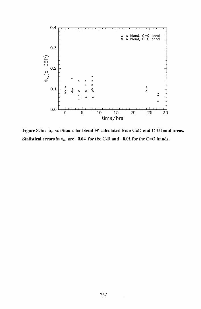
0.4 I .. I I I I I
0 W blend, C=O band 6 W blend, c-o band
0.3 - -
,-..... Q_
m 0 I 0.2 - -
--o ...._.... > "' 0 "' -e- "' "' "'
0 0
0.1 "' A - A 0 -0 0 0 0 0 0 0 0 0
0 0
"' b. A
"' 0.0 I I I I I I
0 5 10 15 20 25 30 time/hrs
Fngure 8Aa: <Pav vs t/lhours for bHendl W calclllllatedl from C=O and C-lD baRlld areas.
Statistical errors un <Pa'' are --'{),(b.:g for the C-D and ~o.m. for the C=O bands.
267

0.4
0 . .3
--------0
Q_ 0
CD A 0 0 0 I 0.2 A
A """0 A ....___.,
> 0
-e-
0.1
0
0
A
10
0 l:;.
20 time/hrs
y y
0
blend, C=O band blend, c-o band
A
0
.30 40
!Figure 8Aib: <l>av vs t'hours for blend Y calculated from C=O and CoD lbandl areas.
Statistical errors in <l>av are -O.Ot:! for the C-D and -O.O.ll. for the C=O bands.
0.4
0 z blend, C=O band l:;. z blend, C-0 band
0 . .3
,.........., Q_
CD 0 I 0.2 "' -o 0 ....___., "' "' "' > "' "' 0 "' 0 0 0 0
-& A 0 0 A
0.1
100 200 300 400 500 600 time/hrs
!Figure 8.4c: <l>av vs t/hours for blend Z calculated from C=O andl C-ID !band areas.
StatisticaR erron·s in <l>av are -0.04 for the C-D and -O.O.ll. for the C=O bands.
268

Average values of <Pav calculated over the whole time range from the C-D and C=O bands
are 0.10(4) and 0.09(1) respectively, if it is true that there is no underlying variation in
the volume fraction of d-DBP then these values give an indication of the random error in
the measured <Pav· Blend Y shows a decrease in <Pav as a function of time, this is clear in
the data from the C=O band but not the C-D band. Finally blend Z, with initially 0.30
volume fraction d-DBP, shows a clear decrease in <Pav from both C=O and C-D bands
over the first -100 hours subsequently a plateau value of <Pav = 0.14 is reached, within the
experimental error this level is maintained up to at least -600 hours (or 25 days).
Figure 8.5 shows a selection of the reflectivity profiles, R vs Q, obtained for the
blends W, X, Y and Z as a function of time after spin casting. The reflectivity data
generally exhibit Kiessig fringes characteristic of the fum thicknesses, the exceptions to
this are the data for the X and Y blends for times less than 24 hours. The absence of
fringes indicates that the scattering length density of the polymer film (plus d-DBP) is
close to that of the silicon substrate, this is expected to occur when then the average
volume fraction of d-DBP in the film, <Pav, is -0.18.
TI1e reflectivity of the W blend changes very a little as a function of time, in
contrast to the Z blend where substantial changes are observed. The clearest of these
changes is a shift in the critical edge to lower Q values at longer times, this corresponds
to a decrease in the bulk volume fraction of d-DBP. There is also a slight increase in the
fringe spacing which suggests that the films are becoming thinner. Trends in the X and
Y blend data are more difficult to discern, although there is a slight shift in the location
of the critical edge to lower Q values for theY blend.
The reflectivity data were analysed using two methods, the maximum entropy
program VOLFMEM was used to obtain free form fits with a pixel size of -15A (this
corresponds to -50 pixels per film) and internal smoothing of lOOA. Secondly a number
of multilayer fits were made using PHOENIX. Models with up to three uniform layers
on top of a lSA silicon dioxide layer were fitted. The roughness' at the air-polymer,
polymer-Si02 and Si02-Si interfaces were fixed at sA. The fit quality for the PHOENIX
multilayer fits will be measured in terms of the fit index, defined in section 4.3.3, which is
not identical to the more commonly used 'nonnalised X2 parameter'. Table 8.3 shows
the correspondence between the normalised X2 parameter and the fit index, obtained for a
selection of PHOENIX (multilayer fits).
269

0
-2
,.---.... 0:::: .....__., ~ -4
01 0
__j
-6
-8
0.00 0.02 0.04 0.06 o;.&.-1
· · · ·_· · 0 hours 0 12 hours 1'1 11 days x 17 days
0.08 0.10
Figure 8.5a: Reflectivaty data for selected blend! W samples, ermll'S fmm Poisson
statistics shown for WOhrs. Successive datasets offset by -:D.. for clarity.
0
-2
,.---.... 0:::: .....__., ~ -4
01 0
__j
-6
-8
0.00 0.02 0.04 0.06 o;.&.-,
······ 0 hours 0 24 hours 1'1 11 days x 17 days
0.08 0.10
JF'igure 8.5b: IReflectivity data for lblend X samples, errors from Poisson statistics
shown for XOhrs. Successive datasets offset by a:D.. for clarity.
270

0
-2
......---. 0::: '--" ~ -4
01 0 _j
-6
-8
0.00 0.02 0.04 0.06 0/A- 1
··-···0 hours 0 24 hours 1::. 11 days x 17 days
0.08 0.10
Figure 8.5c: Reflectivity data for selected! Y samples, ermrs from Poisson statistics
shown for \'Ohrs. Successive datasets offset by -1 for clarity.
0 --... ... ······0 hours 0 6 hours 1::. 12 hours X 24 hours
-2 ¢ 4 days ., .. ·····. * 11 days
0 17 days , .. ......---.
-4 I 'o 0::: I
,,, '--" 111
0
01 0 0
0 -6 1>.1:. _j /j,
-8
-10 D .,., D 00
" a
0.00 0.02 0.04 0.06 0.08 0.10 0/A_,
Figure 8.5d: Reflectivity data for selected! Z samples, ermrs from Poisson statistics
shown for ZOhrs. Successive datasets offset by -1 for clarity.
271
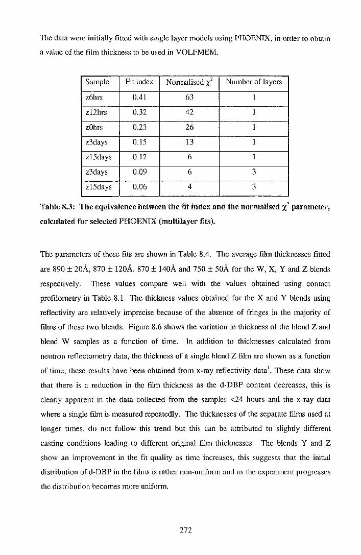
The data. were initially fitted with single layer models using PHOENIX, in order to obtain
a value of the film thickness to be used in VOLFMEM.
Sample Fit index Nonnalised X2 Number of layers
z6hrs 0.41 63 1
z12hrs 0.32 42 1
zOhrs 0.23 26 1
z3days 0.15 13 1
z15days 0.12 6 1
z3days 0.09 6 3
z15days 0.06 4 3
Table 8.3: The equivalence betweeltll the fnt index and the 111ormaHsed X2 parameter,
calcaRiatedl for seBected IPJHIOlENll.X (multnnayer fats).
The parameters of these fits are shown in Table 8.4. The average film thicknesses fitted
are 890 ± 20A, 870 ± 120A, 870 ± 140A and 750 ± 50A for the W, X, y and z blends
respectively. These values compare well with the values obtained using contact
profilometry in Table 8.1 The thickness values obtained for the X and Y blends using
reflectivity are relatively imprecise because of the absence of fringes in the majority of
films of these two blends. Figure 8.6 shows the variation in thickness of the blend Z and
blend W samples as a function of time. In addition to thicknesses calculated from
neutron reflectometry data, the thickness of a single blend Z film are shown as a function
of time, these results have been obtained from x-ray reflectivity data'. These data show
that there is a reduction in the film thickness as the d-DBP content decreases, this is
clearly apparent in the data collected from the samples <24 hours and the x-ray data
where a single film is measured repeatedly. The thicknesses of the separate films used at
longer times, do not follow this trend but this can be amibuted to slightly different
casting conditions leading to different original film thicknesses. The blends Y and Z
show an improvement in the fit quality as time increases, this suggests that the initial
distribution of d-DBP in the films is rather non-unifonn and as the experiment progresses
the distribution becomes more uniform.
272

Sample code Thickness I A <l>d-DBP Fit index
0.10 wOhrs 953 0.14 0.23
w6hrs 936 0.08 0.30
w12hrs 922 0.07 0.38
w4days 927 0.07 0.21
wlldays 875 0.07 0.33
w17days 962 0.07 0.17
0.17 xOhrs 768 0.18 0.18
x24hrs 793 0.17 0.18
x11days 879 0.12 0.13
x17days 1034 0.13 0.16
0.24 yOhrs 852 0.27 0.38
y6hrs 832 0.26 0.40
y12hrs 1070 0.23 0.36
y24hrs 660 0.20 0.24
ylldays 802 0.14 0.21
y17days 974 0.13 0.15
0.30 zOhrs 827 0.35 0.23
z6hrs 808 0.31 0.41
z12hrs 771 0.26 0.32
z24hrs 738 0.23 0.18
z4days 722 0.18 0.15
zlldays 676 0.13 0.12
z17days 736 0.13 0.12
Table 8.4: Fit parameters for the one layer fits to the reflectivity data, error in <j>d.
DBP iS- 0.02
273

1000 I I I I
0 0
0 0 0
900 I- -ex:( 0 ~
(/) A
(/) 800 A
()) r- -
c A ~ u A
...c 700 I- - + -
E + +
~ +
+ 600 - + + + -
0 Blend w D. Blend z + Blend z (x-ray)
500 I I I I
0 2 4 6 Ln [time/hrs]
!Figure 8.6: IFHm Unncknesses olbtainedl for blends W and Z as a function of time.
Figure 8.7 shows the ~(z) profiles obtained from the reflectivity data using
VOLFMEM, the nonnalised x2 parameters for these fits are shown in Table 8.5. There
is a considerable variation in the fit quality but overall the Z blend fits are the best and
there is a crude correlation between the fit quality and the average volume fraction of d
DBP in the film.
w X y z 0 hour 18.1 4.2 6.2 5.5
6 hours 21.9 - 6.2 7.1
12 hours 6.1 - 9.5 4.4
24 hours - 8.8 6.4 3.7
4days 25.7 - - 7.3
11 days 15.4 26.5 31.7 13.4
17 days 7.1 18.7 19.3 4.4
Table 8.5: Normalised X2 parameters for VOLFMEM fits to reflectivity data.
274

0.30
Q_ 0.25 m 0 I
-o 0.20 c 0
+J 0.15 u 0 L.
'+-
<I) 0.10 E ::l
g 0.05 /
······ 0 hours - -6 hours - · -12 hours -4 days - .. 11 days -- · 17 days
' 0 . 0 0 ..____.__,___,____.____,___,___,____.___,___.___.____.___.__.___._____.____.-----''----"---'
0 200 400 600 BOO 1000
Depth z/A
Figure 8./a: Composition vs depth n>rofnBes olbtainedl for bllendl W samplles as a
function of time, u.nsing VOLFMEM.
0.30
Q_ 0.25 m 0 I
-o 0.20 c 0
+J 0.15 u 0 L.
'+-
<I) 0.10 E ::l
0 0.05 >
0.00 0 200
...... 0 hours - -24 hours - · -11 days -17 days
/I~ ,.· I
··.\ ... ·I '·\·.~-
....... -' . ...... / -. ·, ': \ .............
·~\ \
:. \ ' · ... \ : \
400 600 BOO
Depth z/A 1000
Figure 8./b: Composition vs depth profiles obtained for blend X samples as a
function of time, using VOLFMEM.
275
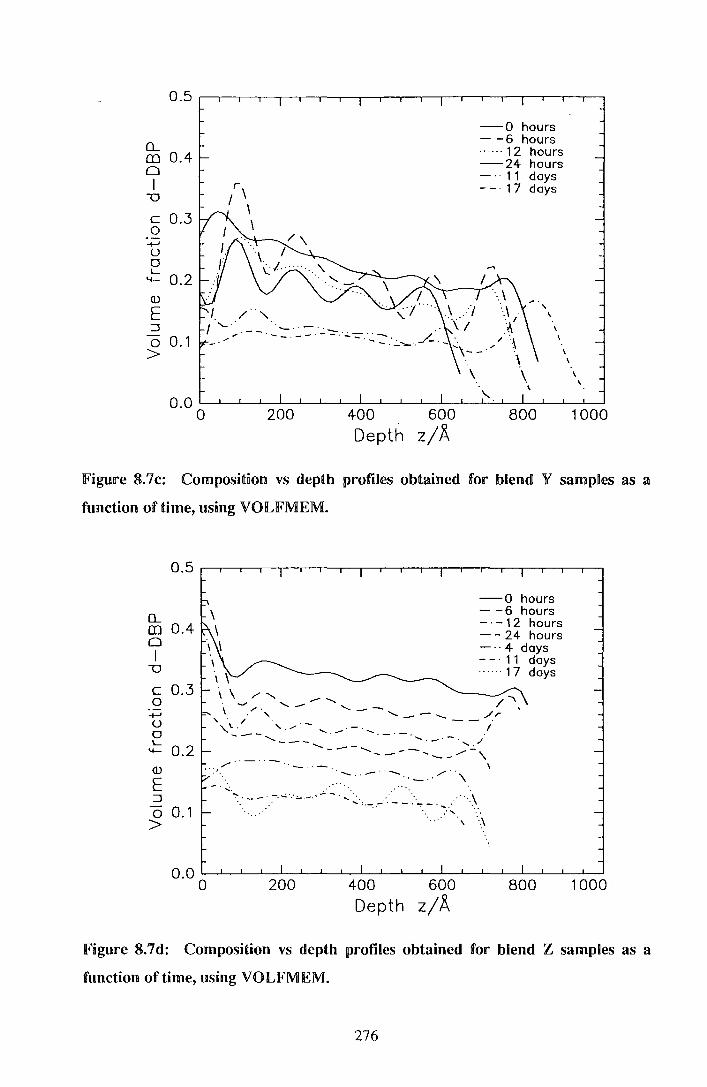
o_ m 0.4 0 I
-o
c 0.3 0
-!-' u 0 L
4- 0.2 (()
E ::l
0 0.1 >
0.0
/""
0 200 400 Depth
600
z/A
-0 hours - -6 hours ·· ···· 12 hours -24 hours - · · 11 days -- · 17 days
I
" 800
I
I \
1000
Figure 8.7c: Composition vs depth profiles obtained! for blend! Y samples as a
function of time, using VOLFMEM.
o_ m 0.4 0 I
-o
c 0.3 0
-!-' u 0 L
4- 0.2 (()
E ::l
0 0.1 >
-0 hours - -6 hours - · -12 hours --24 hours -·· 4 days -- · 11 days ·· ···· 17 days
,... ................ ___ .................. , __ \ _, .. , ........ _-..._
' . / ,\.. -,_ ........ ·- ......... .- ........ ____ _ ---........... ........-·- ........ ./ .......__ _ ___.- ..........
/ ·-··--- .... ......__,-,
.......... --··-... .. _ .. ----··'\ ....:. . ~-:-- .· .. -:-. ....:..·.·.:-.-:--~-- ....... ·~·:.":"": __ ..... _- >~- ......... ·· ·.~\
. .. .... ' ·.-\
I
0.0 ~~~~~~~~~~~~~~~~~~~~~~~ 0 200 400 600 800 1000
Depth z/A
Figure 8.7d: Composition vs depth profiles obtained for blend Z samples as a
function oftime, using VOLFMEM.
276

A number of the composition profiles exhibit high frequency ripples that are probably
due to truncation errors in the data, these ripples are not correlated with the nom1alised
X2 parameter, i.e. do not arise solely in relatively poor or good fits.
The is little evidence for a consistent underlying structure in the <!J(z) profiles,
except for the Y and Z blends at shorter times where there appears to be a small excess
of d-DBP at the air interface, the normalised X2 parameters are, on average, better for
these samples than for the other samples. In the light of the VOLFMEM fit~ all the data
were fitted with two layer models using PHOENIX, the parameters of these fits are
shown in Table 8.6. The symbols <Pn, Zn and crn refer to the volume fraction d-DBP,
thickness and roughness at the bottom of the nth layer, where the first layer is at the air
polymer interface. The two layer models showed a thin well defined layer of d-DBP at
the air-polymer interface, typically -30A thick and with a volume fraction d-DBP up to
0.2 higher than the bulk value. The fit indices for these two layer models are better than
those for the equivalent one layer models. Examples of the <!J(z) profiles obtained using
the two layer models for the Z blend can be found in Figure 8.8.
Figure 8.9 shows a comparison of the fits obtained for selected data using
PHOENIX multilayer fits and VOLFMEM free fonn fits. It can be seen that the one
layer models give good fits up to -0.02k', but beyond this point they under estimate the
reflectivity, the two layer and VOLFMEM fits correct this under estimation. The excess
scattering at higher Q, above the value predicted by the one layer models, is
characteristic of a region of higher scattering length density (i.e. more d-DBP) at the
surface.
Table 8.7 shows the values <Pav obtained using each of the methods of data
analysis, there is good agreement between these values and the values obtained using
A TR spectroscopy. It is interesting to note that the one layer models give a good
estimate of <Pav when compared to the two layer and VOLFMEM fits. Figure 8.10 shows
values of <Pav obtained using two layer models as a function of time, in common with the
A TR data the W blend exhibits no variation in <Pav within the experimental. The average
value is 0.12(3). The X, Y and Z blends exhibit a drop in <Pav to -0.12 over the first 100-
200 hours then <Pav remains constant within the experimental error.
277

Sample q,, ztl A. a, <1>2 z2/ A Fit index.
0.10 wOhrs 0.25 22 36 0.14 944 0.15
w6hrs 0.16 29 33 0.13 959 0.15
w12hrs 0.23 26 5 0.14 957 0.17
w3days 0.17 24 5 0.13 958 0.16
w10days 0.50 20 3 0.12 871 0.11
w15days 0.20 50 26 0.07 922 0.13
0.17 xOhrs 0.32 32 15 0.18 775 0.16
x24hrs 0.32 29 13 0.17 705 0.16
x10days 0.25 32 12 0.12 840 0.10
x15days 0.14 49 9 0.13 998 0.16
0.24 yOhrs 0.45 38 21 0.26 909 0.33
y6hrs 0.56 32 16 0.25 685 0.27
y12hrs 0.42 49 15 0.21 627 0.25
y24hrs 0.23 333 164 0.14 236 0.09
y10days 0.41 33 9 0.13 825 0.16
y15days 0.24 30 14 0.12 791 0.14
0.30 zOhrs 0.55 26 9 0.34 792 0.16
z6hrs 0.60 41 9 0.29 752 0.15
z12hrs 0.52 36 7 0.25 722 0.15
z24hrs 0.42 31 11 0.22 695 0.13
z3days 0.36 24 12 0.18 700 0.14
z10days 0.28 33 13 0.13 641 0.09
z15days 0.44 27 7 0.13 712 0.08
Tabne 8.6: Fit parameters for PHOENIX (two layer models) fits to the reflectivity
data.
278

lPav
Sample VOLFMEM 1layer 2layer Average
0.10 wOhrs 0.12 0.14 0.14 0.13(1)
w6hrs 0.09 0.08 0.13 0.10(3)
w12hrs 0.08 0.07 0.14 0.10(4)
w3days 0.09 0.07 0.13 0.10(3)
w10days 0.11 0.07 0.12 0.10(3)
w15days 0.07 0.07 0.07 0.07(0)
0.17 xOhrs 0.16 0.18 0.18 0.17(1)
x24hrs 0.15 0.17 0.17 0.16(1)
xlOdays 0.11 0.12 0.12 0.12(1)
x15days 0.11 0.13 0.13 0.12(1)
0.24 yOhrs 0.23 0.27 0.26 0.25(2)
y6lu-s 0.20 0.26 0.25 0.24(3)
y121u·s 0.18 0.23 0.21 0.21(3)
y24hrs 0.18 0.20 0.17 0.18(2)
y10days 0.11 0.14 0.13 0.13(2)
y15days 0.11 0.13 0.12 0.12(1)
0.30 zOhrs 0.33 0.35 0.34 0.34(1)
z6hrs 0.30 0.31 0.29 0.3(1)
z12hrs 0.26 0.26 0.25 0.26(1)
z24hrs 0.22 0.23 0.22 0.22(1)
z3days 0.17 0.18 0.18 0.18(1)
z10days 0.12 0.13 0.13 0.13(1)
z15days 0.13 0.13 0.14 0.13(1)
'fable 8.7: Values of <Pav obtained using the different methods of data analysis,
along with am average value with the standard deviation.
279

o_ m 0.8 0 I
-o
c 0
+-' u 0 L
4--
Q)
E :::::1 -0 >
0.6
0.4
0.2
- ...... I \ r· \ ...... '\ .. :_, \
·· .. \\ \
-Z6hrs - -Z12hrs - · -Z24hrs · ····· Z3days -· Z15days
····\ ·,. ~ .-=. .-=. .-=. :-=. .-=. .-=. .-=. :-=. :-=. .-=. .-=. .-=. :-=. .-=. :-:: .-=. .-=. :-:: .-=. .-=. . , ................................................ ·····································
50 100 150 200 250 300
Depth /'A
Figure 8.8: <j>(z) profiles for the Z blend, derived from two layer model fit
parameters for neutron reflectivity data.
0
-1 .,-...... 0::: ..____.....
s -2 CJl 0 _j
-3
-4
0.02
······experimental - 1 layer model - -2 layer model -·-Free form model
0.04 0.06 0.08 o;'A-1
0.10
Figure 8.9a: A comparison between the ZOhrs reflectivity data (with errors from
Poisson statistics) and model fits from one layer, two layer and free form fits.
280

0.02
· ·· · ·experimental - 1 layer model - -2 layer model - · -Free form model
0.04 0.06 0.08 0/A-1
0.10
Figure 8.9b: A comparison between the Z24hrs reflectivity data (with errors from
Poisson statistics) and model fits from one layer, two layer and free form fits.
0
-1
,---..... 0:::: -2
'-...../ 0 ~
O"l 0 -3 _j
-4
-5
0.02
· · · · · · experimental - 1 layer model - - 2 layer model -·-Free form model
0.04 0.06 0.08 0/A_,
0.10
Figure 8.9c: A comparison between the Zl7days reflectivity data (with errors from
Poisson statistics) and model fits from one layer, two layer· and free form fits.
281

0.02
······experimental - 1 layer model - -2 layer model - · -Free form model
0.04 0.06 0.08 o;,&.-1
0.10
Figure 8.9d: A comparison between the W12hrs reflectivity data (with errors from
Poisson statistics) and model fits from one layer, two layer and free form fits.
0.4
0 Z blend 0 6. Y blend
+ X blend
0.3 x W blend
0
.,--..... t;. o_ LO
m 0 0
t;.
I 0.2 -o + 0 ............, ,.
> 0
-e- XX 0 X )( Ct. + + X t;.
0.1 X
0 100 200 300 400 500
time/hrs
Figure 8.10: .Pav vs time/hours for the W, X, Y and Z blends, measured using
neutron reflectivity data, two layer models. Statistical error in cpa,, is -0.02.
282

8.3 Discussion
In the previous section it was found that the average volume fraction of d-DBP,
<l>av, in thin films of polystyrene decreases as a function of time and reaches a constant
value of -0.13. Additionally it was found that a thin layer of d-DBP ( -30A) fanned at
the air-polymer interface. The relatively large loss of this plasticiser from the substrate
polymer is known2 and is one of the reasons that DBP is no longer used industrially as a
plasticiser.
Three factors will be involved in detennining the rate at which <l>av decreases,
these are the evaporation rate, a, the mutual diffusion coefficient, D11., and the film
thickness, 1. The type of behaviour observed will depend on the relative sizes of these
factors. Two regimes arising from the relative sizes of a and Dm can be envisaged:
(i) where the evaporation rate is larger or comparable in size to the diffusion rate.
(ii) where the evaporation rate is small compared to the diffusion.
Intuitively it can be seen that, in the absence of any other factors, films in regime (i) will
exhibit some sort of variation in the volume fraction of d-DBP as a function of depth
whereas those in regime (ii) will exhibit no such variations because immediately d-DBP is
lost from the smface region it is replaced by material from the bulk of the sample.
Crank3 discusses the mathematics of analysing diffusion data in a wide range of
situations. The simplest of these is the sorption-desorption case, where it is assumed that
the evaporation rate a. is large (case (i)) and so the rate of mass loss from the film is
detennined by the mutual diffusion coefficient, Dm. A crude estimate of Dm can be
obtained using the expression below:
Equation 8.3
where tc is the characteristic time required for the value of <l>av to drop half way to it's
equiliblium value. Using a value of 1 = 700A and tc = 24 hours this would imply a value
of Dm = 3x10-17 cm2 s-1• Such a value of Dm for d-DBP would be far smaller than values
for di-octyl phthalate in natural rubber4 (Dm = 1.8xl0-8 cm2 s-'), toluene in poly (vinyl
acetate)5 (D,n = 10-9-10-7 cm2 s-1) and water in poly (styrene-co-acrylonitrile)6 (Dm- Hr
283
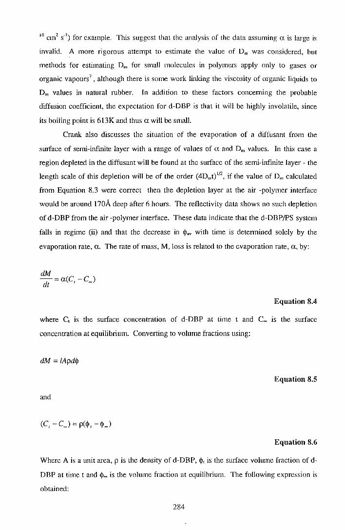
10 cm2 s-1) for example. This suggest that the ;malysis of the data assuming a is large is
invalid. A more rigorous attempt to estimate the value of 0 111 was considered, but
methods for estimating Dm for small molecules in polymers apply only to gases or
organic vapours7, although there is some work linking the viscosity of organic liquids to
Dm values in natural rubber. In addition to these factors concerning the probable
diffusion coefficient, the expectation for d-DBP is that it will be highly involatile, since
its boiling point is 613K and thus a will be small.
Crank also discusses the situation of the evaporation of a diffusant from the
surface of semi-infinite layer with a range of values of a and Dm values. In this case a
region depleted in the diffusant will be found at the surface of the semi-infinite layer - the
length scale of this depletion will be of the order (4D111t)112
, if the value of Dm calculated
from Equation 8.3 were correct then the depletion layer at the air -polymer interface
would be around 170A deep after 6 hours. The reflectivity data shows no such depletion
of d-DBP from the air -polymer interface. These data indicate that the d-DBP/PS system
falls in regime (ii) and that the decrease in cl>av with time is detennined solely by the
evaporation rate, a. The rate of mass, M, loss is related to the evaporation rate, a, by:
Equation 8.4
where C is the surface concentration of d-DBP at time t and C~ is the sm"face
concentration at equilibrium. Converting to volume fractions using:
dM = !Apdcj>
Equation 8.5
and
Equation 8.6
Where A is a unit area, p is the density of d-DBP, cj>1 is the smface volume fraction of d
DBP at time t and 4>"" is the volume fraction at equilibrium. The following expression is
obtained:
284
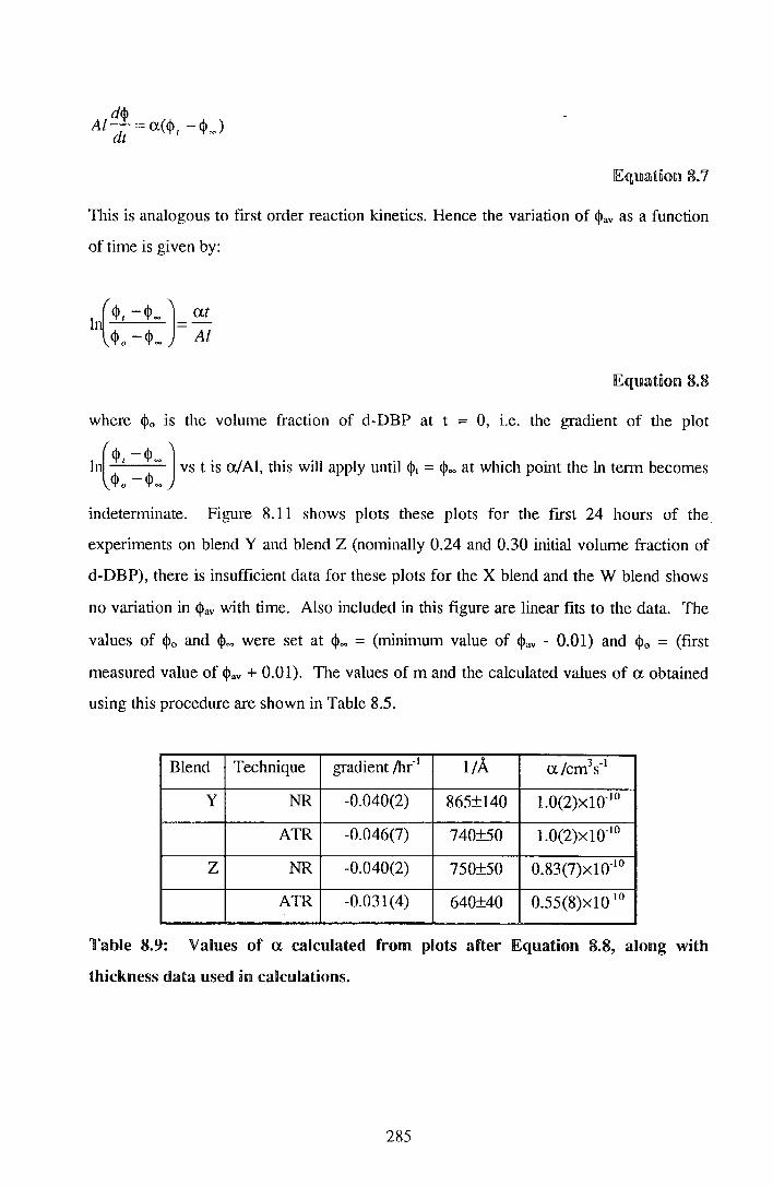
This is analogous to first order reaction kinetics. Hence the variation of <l>av as a function
of time is given by:
Equatnon 8.8
where <l>o is the volume fraction of d-DBP at t = 0, i.e. the gradient of the plot
ln(lj> 1 - 4> ~ J vs t is a/ AI, this will apply until 1)>1 = 4>~ at which point the ln term becomes
<l>o -<!>~
indetenninate. Figure 8.11 shows plots these plots for the frrst 24 hours of the
experiments on blend Y and blend Z (nominally 0.24 and 0.30 initial volume fraction of
d-DBP), there is insufficient data for these plots for the X blend and the W blend shows
no variation in <l>av with time. Also included in this figure are linear fits to the data. The
values of <l>o and <!>~ were set at <l>oo = (minimum value of <l>av - 0.01) and <l>o = (frrst
measured value of <l>av + 0.01). The values of m and the calculated values of a obtained
using this procedure are shown in Table 8.5.
Blend Technique gradient /h(1 l!A a/cm3s-1
y NR -0.040(2) 865±140 1.0(2)x1 o-IO
ATR -0.046(7) 740±50 1.0(2)Xl0-IO
z NR -0.040(2) 750±50 0.83(7)x1 o-10
ATR -0.031(4) 640±40 0.55(8)x10-10
Table 8.9: Values of a calculated from plots after Equation 8.8, along with
thickness data used in calculations.
285

0.0 0
0 ATR data 0
~ 6 NR data .0.
.,.-...... " -Fit to ATR ,..--..... " --Fit to NR
8 " -B- ' I (}. 0 0 ' -B- -0.5 ' .....___, ' ~ ' .,.-...... ' 8 ' -B- ' I ' -B- ' .....___, ' .....___,
' -1.0 ' c ' -' Q.
' ' ' ' 0 10 20 30
Time /hrs
JFfiguure §.ll.Jla: !Plots of 1_( <I>,-<!>~ J vs t for theY blend, usnrng A'flR aml! NJR d!ata 1\<J>o -<J>~
witlh linear fits.
.,.-......
.,.-...... 8
-B-1
0
0.0
-B- -0.5 .....___, ~ .,.-......
8 -B-
1 -& .....___,
.....___,
c -'
-1.0
0
0
0
" ' o'-
' .0. ' 0 '
0
' ' ' .0. ' ' ' ' ' '
0
0 ATR data t:. NR data
-Fit to ATR --Fit to NR
0
' .0.
'
10 20
Time /hrs
' ' ' ' ' ' 0
'
30
' ' '
Figure 8.Ub: !Plots of l_(<j>, -<!>~) vs t for the Z blend, using ATR. and NR data 1\<J>o -<J>~
with Binear fits.
2R6

To put these values of a in context, one would expect from these results that in an 8cm
diameter circular dish with a 1 mm thick layer of d-DBP in the bottom that over a period
of one week only 0.07% of the d-DBP would evaporate. This assumes that the
evaporation rate of pure d-DBP is the same as that for d-DBP in polystyrene. A further
experiment that could be done would be to measure the evaporation rate for pure d
DBP, this is not straight forward since the expected effect is very small and DBP absorbs
atmospheric water.
lin the preceding analysis it was assumed that the polystyrene + d-DBP film
thickness was constant, this is known not to be true but including the effect of a film
thickness dependent on <!lav means that no simple analytical fonn for <!lav = f(t) is available.
Figure 8.12 shows a comparison of <!lav vs ln [time /hours] for the approximation used
above and for a more exact solution which allows for the variation of film thickness with
<!lav- Fitting this expression manually to the Z blend NR data a value of a = 1.5(2) xl0-10
cm3s·1 is obtained. Neither of these analyses include the effect that a surface composition
different from the bulk composition might have.
> 0
-e-
()_
m 0 I
""0
c 0
+-' 0 0 I... 4-
(I)
E ::J
-0 >
0.4
0.3
0.2
0.1
0.0 0
Constant Film thickness Variable film thickness
0 Z blend NR data
2 4 6 Ln [time /hours]
Figure 8.Jl2: $av vs Ln [time /hours] for the Z blend along with theoretical
predictions from two models, a parameter is fixed at optimum value for variable
thickness model.
287

These experiments have shown that neutron reflectometry is not an ideal method
for detennining diffusion coefficients for such small molecules. If the evaporation rate
had been large then the diffusion coefficient could have been obtained from the total
mass loss from the fllm using the sorption-desorption equations discussed by Crank, but
then this could also have been done using A TR and although the statistical error in A TR
is rather larger the measurement time is smaller and so larger diffusion coefficients can be
examined. If the diffusion coefficient were to be detennined by examining the profile
shape at the air interface then again neutron reflectometry would only be suitable for
relatively small diffusions coefficients (<10-14 cm3 s-1) because, given the minimum
measurement time the length scale of the profile would be such that NR was insensitive
to it at larger values of Dm.
It is likely that the mutual diffusion coefficient of DBP in PS would vary
markedly with composition. Zhang and Wang8 have shown that the diffusion coefficient
of camphorquinone in polystyrene plus dioctyl phthalate varies markedly with the
concentration of di-octyl phthalate for temperatures above the glass transition
temperature of the polymer, which is influenced by the concentration of the di-octyl
phthalate. Xia, Whang and Li9 have shown that the diffusion coefficient for
camphorquinone in poly (aryl ether ether ketone) exhibits a clear change in behaviour as
the temperature drops below Tg. In the system studied here the DBP plasticises the
polystyrene. It was found using differential scanning calmimetry (DSC) that for a
volume fraction DBP of 0.30 the Tg is -277K (compared to Tg = 376K for the pure
polymer). Data in the literature2'8 indicate a linear relationship between Tg and volume
fraction DBP, so that over the composition range studied here the films change from
being above their T g at room temperature for $av = 0.30 to below T g with $av = 0.1 0.
The Tg becomes equal to room temperature when $av""' 0.23. If diffusion data had been
obtained then it could be analysed in the context of the free volume models of Vrentas
and Duda10•
It was found that the d-DBP did not continue to evaporate from the polystyrene fihn
until there was no d-DBP left, instead it was found that for the W blend there was no
evaporation and for the other blends the average volume fraction decreased until a
constant value of -0.12 was reached. If this level of $av represents an equilibrium value
then it would be expected that at this point the chemical potential of the d-DBP in the
2R8

film will be equal to that of the d-DBP vapour above the f.tlm. The chemical potential of
the d-DBP in the film, IJ.r, can be calculated from Flory- Huggins theory:
llJ-Ilt ( 1} ___:__:.___ = ln q> + 1 - - 1 - q>) + X FH (1- q>) 2
RT r
EqUJtatfiolll 8.9
where r = N/Ns is the ratio of the degree of polymerisation of the polymer to the effective
degree of polymerisation of the solvent, comparing the segment volume of polystyrene (
= 1.653xl0-22 cm3) and the molecular volume of d-DBP (= 4.33x10⁻²² cm3
) indicates that
r"'" 3400. R is the gas constant(= 8.315 J K 1 mor1) and T is the absolute temperature.
q> is the volume fraction of d-DBP. XFH is the Flory- Huggins interaction parameter and
is not known. The chemical potential of the d-DBP vapour, IJ.v, is given by:
Equation 8.10
where Po is the pressure in the standard state and Pv is the vapour pressure. The vapour
pressure can be estimated from the boiling point (or the vapour pressure at another
temperature) using the Clausius- Clapeyron equation:
dIn Pv 11H,."P dT RT 2
Equation 8.11
where .1Hvar is the enthalpy of vaporisation of d-DBP, integrating this to give:
• -c Pv = P e
Equation 8.12
where:
c = ~V<lp (~ - ;. )
Equation 8.13
289

p *is a known vapour pressure at temperature T*. Two possible combinations ofT* and
p* are T* = 613K and p* = 760 mmHg (from the boiling point) and T* = 479K and p* =
20 mmHg (data in reference 11 ). The enthalpy of vaporisation can be estimated from
Troutons rule (L~Hvap""' 85 J K 1 mor1 x T), for DBP this corresponds ~Hvap""' 52 KJ mor
1• These values of p * and T* indicate a vapour pressure of 0.005 ffilnHg for dibutyl
phthalate at room temperature, this indicates a value of (J.lv-1-lv)/RT = -12. In principle
we should be able to estimate a value of )(A-1 by setting <P = 0.12 in Equation 8.8 and
varying XFH until the chemical potential of matches that of the vapour. This gives a value
of XA-1 = -13, which is unfeasibly large in magnitude when compared to values of XA-1
obtained for other solvent - polymer systems which generally lie in the range -0.5 to 1.0.
This large discrepancy between the expected and calculated values of Xffi prove that the
d-DBP in the film is not at equilibrium with the region above the film. Clearly a large
number of assumptions have been made in these calculations, including the assumption
that the system is closed and the numerous assumptions made in estimating the vapour
pressure of d-DBP at room temperature. However, in an open system the vapour
pressure of d-DBP would tend to be lower than in the closed system and hence the
equilibrium <l>av would be even less.
Neutron reflectometry (NR) can provide unique infonnation on the distribution
of d-DBP in polystyrene films. This is because the NR sample is kept in ambient
conditions of temperature and pressure during measurement, in contrast to other surface
analysis techniques SIMS, NRA and XPS where the sample is placed in a vacuum for
measurement. Early on in this work it was found that, when examined using SIMS or
XPS, the surface of the DBP plus polystyrene film was completely devoid of DBP. The
explanation for this is that despite its high boiling point under high vacuum the DBP is
sufficiently volatile to boil out of the sample, at least up to the XPS or SIMS probe depth
(i.e. -50A).
Although the observed surface excess is very small we can be fairly confident of
its existence. The surface excess is clearly visible in the VOLFMEM fits to the Z blend,
where the fit quality is high and there are no unphysical structures in the bulk of the film.
The one layer models under estimate the reflectivity of the samples at higher Q, whilst
the two layer models fit the data rather better with a thin layer rich in d-DBP at the air
polymer intetface.
290
If either the smface excess or the difference ($1 - $2), where $t and $2 are the volume
fractions of DBP in the first and second layers of the two layer models, are plotted
versus $av (see Figure 8.13) then the data can be fitted with a straight line passing
through the origin, which is what would be expected for surface enrichment behaviour.
The gradients of these straight lines are 36(6) and 0.9(1) for the surface excess and the
difference ($t- $2) respectively. There is rather a large scatter in the values of ($1 - $2)
and the surface excess for the lower values of $av· Such results are not unprecedented,
similar work on a tackifier in polyisoprene12 which also shows an excess at the air
polymer interface.
There are two reasons for expecting the excess of d-DBP at the air-polymer
interface- firstly DBP has a lower surface energy than polystyrene the values are 33.1 mJ
m-2 and 40.7 mJ m-2 respectively13• Secondly the DBP, a small molecule, loses less
entropy on being confined to the air-polymer interface then the polystyrene. Self
consistent field theory models, using a value of ,!!:,:y calculated from the literature values of
the surface energy and values of N = 100 for the non-absorbing polymer (= PS) and N =
3 for the absorbing species (= DBP) and values of X of 0 and 0.2, do show an excess of
DBP at the air-polymer interface, see Figure 8.14. These models show that the predicted
surface excess is qualitatively similar to that observed in the experimental system,
although the layer thickness is somewhat thinner. Discrepancies between these models
and the experimental data are not unsurprising since the programs used in calculating the
theoretical profiles were not written with such a situation in mind.
291

20
+ data
Q_ -linear fit
m 0 15 I
-o
(f) (f) (])
10 u X (])
(])
I u a
'+- 5 I._
::J (f)
0 ~~~~~~~~--~~~~~~~~--~~~~~ 0.0 0.1 0.2 0.3 0.4
Average volume fraction d-DBP
!Figure §.13a: Surface excess vs <l>av calculated from the two Hayer modlel fits to the
reflectnvnty data. lLine ns a straight line fnt wnth the intercept fixed at zero.
<"' -e-1
0.4
0.3
-e- 0.2
0.1
+ data -linear fit
0.1 0.2 0.3 Average volume fraction d-OBP
0.4
Figure 8.13b: (<!>1 - <!>2) vs <l>av calculated from the two layer model fits to the
reflectivity data. Line is a straight line fit with the intercept fixed at zero.
292
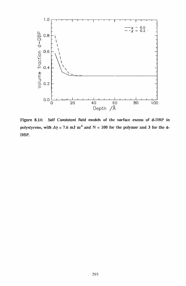
1.0
-x = 0.0
Q_ - -x = 0.2
m 0.8 \ 0 \ I ""0 \
0.6 \ c \ 0 +-' \ u \ 0 L
0.4 \ 4-
\ (1) \.
E ::J - 0.2 0 >
0.0 0 20 40 60 80 100
Depth /A
JF'ngure 8.M: Self Consiste~rnt field models of the surface excess of da!l)JBJP in
polystyrene, wfith f).:y = 7.6 m.J1 m-2 and! N = WO for the poHymer amen 3 for the d-
DJBJP.
293

8.4 Conclusions
Neutron reflectometry and attenuated total reflection infra red spectrometry both
indicate that the average volume fraction of d-DBP in a -800A polystyrene film
decreases as a function of time after the film is spun cast. The characteristic time of this
decrease is around 24 hours and the decrease appears to stop when the average volume
fraction of d-DBP reaches -0.12. It was found that for films with an initial volume
fraction of 0.10 d-DBP lost no d-DBP over a period of 17 days, within the experimental
error. Calculations show that this level of d-DBP is far higher than would be expected at
thennodynamic equilibrium. The lack of a depletion zone near the surface of the film
implies that the decrease in <l>av was determined by the rate of evaporation a, a value of a
= l.Ox10-10 cm3 s-1 was calculated.
Neutron reflectometry results showed that there was a small excess of d-DBP at
the air-polymer interface, this excess was confined to a layer -30A thick. This excess
can be modelled broadly using the self consistent field theory of Shull with values of the
surface energy difference between dibutyl phthalate and polystyrene found in the
literature.
294

8.5 /Re1erences 1or Section 8.
1 . R.W. Richards, unpublished results.
2. J.K. Sears, N.W. Touchette in 'Encyclopedia of Polymer Science and Engineering
Supplement Volume', J. Wiley & Sons, 1989.
3. J. Crank, 'The Mathematics of Diffusion 2nd ed. ', Oxford Science Publications,
1975.
4. E. Southern, A.G. Thomas, Transactions of the Faraday Society, 63, :ll.967, 1913.
5. J.S. Vrentas, J.L. Duda in 'Encyclopedia of Polymer Science and Engineering Vol. 5
2nd ed. ', J. Wiley & Sons, 1986.
6. G.T. Fieldson, T.A. Barbari, Polymer, 34(6), :ll.993, 1146.
7 . D.W. Van Krevelen, 'Properties of Polymers 3rd ed.', Elsevier, 1990.
8. J. Zhang, C.H. Wang, Macromolecules, 21, :ll.988, 1811.
9. J.L. Xia, C.H. Wang, B.Y. Li, Macromolecules, 21, 1990,2739.
10. S.L. Vrentas, J.L. Duda, Journal of Polymer Science, Polymer Physics Edition, 15,
:ll.977, 403.
11 . R.C. Weast, 'CRC Handbook of Chemistry and Physics 68th ed. ', CRC Press,
1988.
12. X. Li, M.D. Foster, Poster at 'MacroAkron '94' (35th IUPAC Symposium on
Macromolecules, Akron, Ohio, 1994).
13. J. Brandrup, E.H. Immergut, 'Polymer Handbook 3rd ed.', J. Wiley & Sons, 1989.
295

Results from each of the systems studied have been summarised at the end of
each section, so the intention now is to draw some general conclusions and make
suggestions for further work.
The X data for the syndiotactic d-PMMA/h-PMMA blends exhibited the
composition variation predicted for 'repulsive' blends. Further experiments in this area
would include a more in depth study of the variation of X with chain length disparity, an
ideal experiment would be to use a fixed temperature -440K and volume fraction d
PMMA -0.5 and vary the ratio No:NH from 1:100 to 1:1 keeping the h-PMMA
molecular weight fixed at -1,000,000. The motivation for this work would be to provide
a further test for new theories of polymer - polymer thermodynamics. The 'surface
enrichment' study of h-PMMNd-PMMA shows the importance of knowing the
thennodynamics of a blend and screening samples using other techniques before
embarking on a detailed study using NR. Depending on the results of further SANS
work on d-PMMA/h-PMMA it way be worth seeking smface enrichment in symmetric
(NH = N0 ) high molecular weight blends of d-PMMNh-PMMA.
The X data for the PEO/PMMA blends exhibited composition dependence that
would be expected for an 'attractive' blend. It would be useful to examine the
PEO/PMMA system over a wider range of compositions, but a more important question
would be to find the temperature dependence of X at single composition (~ct-PEo = 0.25)
since there is a discrepancy in this between this work and the work of Russell. As a
precautionary note, the exclusion of air bubbles from the SANS samples is critical, this
may be done successfully by holding the samples under vacuum during all of the pressing
procedure and perhaps keeping samples in a dry atmosphere after fabrication. Note that
air bubbles were not apparent in the 'as prepared' samples.
The study of the surface enrichment behaviour of PEO/PMMA can best be
described as an 'interesting start', it would appear that the behaviour observed is not
described by current theory. This system is worthy of further study because both
components can be prepared with good control of molecular weight and narrow
molecular weight distributions in both hydrogenous and deuterated fonn, clearly the
hope would be to drive further theoretical developments using results from this blend.
296

However the extreme roughness of the samples makes the analysis of the NR data
difficult. It would be useful to re-examine the d-PEO/h-PMMA blend using NR in the
melt state where the air - polymer interface should be rather smoother and with NRA
optimised to the polymer - substrate interface.
Clearly d-PS(F), d-PS(F2) I h-PS systems have produced the most complete
results - this is in large part due to the substantial amount of infonnation on the surface
emichment and thennodynamics of the d-PS/h-PS blends that is in the literature. It was
gratifying to find that the SCF theory was able to describe the brush fanning behaviour
of these blends, using data in the literature on surface energy and solubility parameters.
However it should be noted that the effect of the perfluorohexane end group is relatively
small when compared to the size of the effect dtiven by smface energy differences in
heteropolymer blends. Work is already in progress to study the effect of the molecular
architecture of the d-PS(F), i.e the location of the fluminated group(s), on surface
segregation behaviour of systems of this sort.
In the d-DBP/PS system an attempt was made to apply some of the methods and
ideas from the other systems to an industrially more relevant situation, the use of d-DBP
was imposed due to considerations of ease (and cost) of synthesis. The results show
some promise for future work on this system, one possibility now that the feasibility of
these experiments has been shown would be to try to synthesise a higher molecular
weight perdeuterated phthalate, this would reduce problems of evaporation loss and
possibly allow the use of high vacuum techniques (such as XPS or SIMS), if the sample
were sufficiently cooled.
297

i (!]. Appendices
"'ff 0. 1 Glossary o1 Symbols
Roman alphabet
a
A
A
AA
An
Ac-o
Ac-H
Ac-x
A e--o
b
b
B
statistical segment length
parameter in the WLF equation
parameters of fits to X of the fonn X= A+Bff
unit area (Section 8.3 only)
infra red absorption in A TR mode
nonnalisation constant for <!>A in SCF theory
normalisation constant for <l>n in SCF theory
integration of C-D stretch peak IR absorption band
integration of C-H stretch peak IR absorption band
either Ac-o or Aco=0
integration of C=O stretch peak IR absorption band
cube root of the segmental volume, V111
single atom nuclear scattering length (Section 3.1.1 only)
nuclear scattering length of component i, (including i = H, D, A, B)
parameters of fits to X of the fonn X= A+Bff
parameter arising from the Clausius - Clapyeron equation
parameter in the WLF equation
parameter in the WLF equation
concentration at time, t.
concentration at t = oo
spacing for Bragg peak
penetration depth for A TR spectroscopy
effective sample thickness for A TR
sample detector distance in neutron reflectometry
number of neutrons scattered per unit time into solid angle d.Q
parameter used for describing 0, as a function of Mw and T
298

Do
Eo
Esarn
fs( <I> air)
g
go(Rg. Q)
g'o(Rg, Q)
G
h
h
I(Q)
I
k'
k'
L
L
m
average distance between graft points
mutual diffusion coefficient
self diffusion coefficient
electric field amplitude in A TR crystal
activation energy for diffusion
most probable energy in Maxwell- Boltzmann distribution
electric field amplitude in sample
electric field amplitude at A TR crystal I sample interface
surface free energy contribution
coefficient in Taylor series expansion for f,(<J>air)
Debye function for polymer with radius of gyration Rg
modified Debye function for polydisperse blend
crystalline growth rate
Planck's constant
parameter in Schultz- Zimm distribution (section 2.1 only)
coherent elastic neutron scattering
segmental ionisation potential
incident neutron intensity
reflected neutron intensity
total neutron scattering intensity
Boltzmann constant
parameter used for describing Ds as a function of Mw and T
neutron wavevector perpendicular to surface in mediums 0 and 1
incident wavevector (section 3.1 only)
parameter used for describing D. as a function of Mw and T
scattered wavevector (section 3.1 only)
coefficient in expression z * eq = K<j>B
calibration constant for LOQ data
total film thickness
coefficient in expression z*eq = K<J>B +L<j>B2
brush height (section 2.3.2 only)
segment molar mass
rest mass of j (=a, D, p, 3He) (section 3.2 only)
299

M
M· J
n
nair
nps
nS.1111
nsi
N
N
Po
Pv
p
p*
r
rest mass of neutron
mass loss in evaporation I diffusion type experiment
mass variable in Schultz - Zimm distribution
weight average molecular weight
number average molecular weight
layer matrix fort layer in neutron reflectivity optical matrix
product of layer matrices in neutron reflectivity optical matrix
calculations
element of MR
element of MR
neutron refractive index
neutron refractive index in layer j (where j = 0, 1, j)
optical refractive index of A TR crystal (section 3.3 only)
area of one face of a lattice cell in a self consistent field theory
optical refractive index for polystyrene
optical refractive index of a sample (section 3.3 only)
optical refractive index for silicon
Avogadro's constant, or degree of polymetisation of component A
degree of polymerisation of component B
weight average degree of polymerisation of the specified component
number of nuclei in ensemble (section 3.1.1 only)
weight average degree of polymerisation of the deuterated component
weight average degree of polymerisation of the hydrogenous component
number of data points in a neutron reflectivity dataset
effective degree of polymerisation for d-DBP
reference pressure
parameter of jth layer of neun·on reflectivity optical matrix
vapour pressure of DBP
parameter for Schultz- Zimm distribution
vapour pressure of DBP at known temperature T*
distribution functions in self consistent field theory, (i =A, B1, B2 or i)
true scatteting vector (section 3.1 only)
commonly named 'scatteiing vector' (= I Q I) ratio N/N, (section 8 only)
300
ro1
r· J
R
Rn
s1
s2
S(Q)
t
t
tactual
tref
T
u
v
v
V(r)
general position vector
Fresnel reflectivity coefficient between layers 0 and 1.
modified Fresnel reflectivity coefficient for/' layer of neutron
reflectivity optical matrix
atom position vector (section 3.1.1 only)
atom position vector of ith atom in ensemble (section 3.1.1 only)
neutron reflectivity or universal gas constant
radius of gyration of the deuterated component
radius of gyration of the hydrogenous component
radius of gyration of a specified component
equilibrium length used in ~Ge1 calculation (section 2.3.2 only)
model reflectivity (section 3.1.2 only)
measured reflectivity (section 3.1.2 only)
height of slit 1 in neutron reflectometer
height of slit 1 in neutron reflectometer
scattering structure factor
unperturbed mean squared end to end distance
reduced parameter used in surface enrichment theory (section 2.2)
annealing time or time after spin casting
actual annealing time
characteristic time for formation of surface excess
annealing time at a reference temperature
absolute temperature (in K)
temperature at which DBP as vapour pressure p*
crystallisation temperature
glass transition temperature
melting temperature
spinodal temperature
the product RgQ
velocity
segmental volume for a specified component
segmental volumes of components A and B
reference volume
Fermi pseudo potential
301
Vmax
w
w'
X
Xn
z
* z
* Z air
* Z dep
* Zeq
* Zo
* Z si
segmental volume for deuterated and hydrogenous components
volume of lattice cell in self consistent field theory
most probable velocity of neutron in Maxwell- Boltzmann disuibution
velocities ofparticlesj (=a, D, p, 3He) in i (=em or lab) frame of
reference where (section 3.2 only)
parameter in Tanh profile fit
component of mean field
mean fields in self consistent field theory (i = A, B, ext, i, lk, k)
component of mean field (i = A, B)
lattice layer number in self consistent field theory
number of lattice layers in SCF model
distance from air-polymer interface
lattice coordination number
thickness of the nth layer of a multilayer model
parameter in Tanh profile fit
smface excess
smface excess at polymer - air interface
'size' of the depletion zone
equilibrium surface excess
surface excess at t = 0.
surface excess at polymer - substrate intetface
Greek Symbols
a
a
ao
evaporation rate (Section 8 only)
parameter used for describing Ds as a function of Mw and T
polmisability of a deuterated segment
polarisability of a hydrogenous segment
sample I beam angle in NRA experiment
infra red absorption coefficient at wavelength, /...
free energy of end attachment
302

A
A
o(x)
Ors
8nFE
Os
AG
AGe,
AGm
AHvar
ARo
AQ
Ay
All
28
1C
neutron optical path length in / 1 layer of neutron reflectivity optical
matrix
parameter for Schultz- Zimm distribution (Section 5.1.3 only)
wavelength of a neutron or infrared radiation
Dirac delta function
solubility parameter for polystyrene
solubility parameter for poly (tetrafluoroethylene)
thickness of end confinement region in self consistent field theory
Gibbs free energy of a blend, including surface contributions
elastic contribution to the Gibbs free energy of a brush
Gibbs free energy of mixing for a binary polymer blend
Enthalpy of vaporisation
uncettainty in measured reflectivity (section 3.1.2 only)
resolution measured Q (section 3.1.2 only)
surface energy difference
chemical exchange potential
Freed and Bawendi effective interaction energy
nearest neighbour pair potentials where i = A, B, j = A, B.
parameter in self consistent field theory- inversely proportional to
compressibility
angle of reflection in neutron reflectometry
angle of neutron beam relative to surface in jth layer for neutron
reflectivity optical matrix calculation (where j = 0, 1, j)
incident angle for A TR
critical angle (neutrons or electromagnetic radiation)
beam I detector angle in NRA experiment
scattering angle for neutron techniques
compressibility
modified chemical potential (section 2.3.1 only)
chemical potential of DBP in film
reference chemical potential for DBP in film
chemical potential of DBP vapour
303

~', ~~~
tt. bulk tt. hulk 't'A , 't'B
reference chemical potential for DBP vapour
concentration fluctuation correlation length
concentration fluctuation correlation length at coexistence curve
decay length for exponential function in PHOENIX (section 4.3.3) only
mass density
nuclear scattering length density
Foutier transfonn of nuclear scattering length density (as a function of
depth)
dimensionless grafting density
nuclear absorption cross section
nuclear incoherent cross section
roughness of nth interface of a multilayer model
parameter for Schultz- Zimm distribution (Section 5.1.3 only)
volume fraction of the deuterated component or specified component
azimuthal angle in SANS (section 4.2 only)
composition of coexisting components in a binary blend
average volume fraction at t = 0
parameter in Tanh profile fit
average volume fraction at t = oo
maximum volume fraction of deuterated component near the air -
polymer interface
integrated average volume fraction
volume fraction of deuterated component in the bottom of the depletion
layer
volume fraction of deuterated component in the nth layer of a multilayer
model
average volume fraction at time, t.
maximum volume fraction of deuterated component near the polymer -
substrate intetface
volume fractions of component i in lattice layer x (where i = A, B)
(section 2.3.1 only)
bulk volume fractions of components A and B (section 2.3.1)
304

Xm
Xs
Xv
bulk volume fraction
maximum volume fraction of deuterated component near the polymer
substrate inte1face
effective Flory- Huggins interaction parameter
the nonnalised X2 fit parameter
value of X at the coexistence curve
contribution to X arising from mixing at constant volume
enthalpic contribution to xd entropic contribution to xd bulk interaction contribution to attachment energy
smface interaction contribution to attachment energy
the Flory- Huggins interaction parameter
the calculated value of XA-I at the spinodal temperature
contribution to X arising from volume change
305

10.2 Ao!o1iiional Daia
X data for h-PMMA/d-PMMA (section 5.1)
<J>d-PMMA
T!K 0.09 0.29 0.49 0.70
408 1.52E-02 4.74E-03 1.26E-03 1.69E-04
435 2.28E-03 -1.02E-03 -1.19E-03 -1.29E-03
453 -2.28E-03 -3.80E-03 -4.07E-03 -6.47E-04
473 -6.84E-03 -1. 18E-02 -LlOE-02 -3.96E-03
'fablle W.n.: X values obtahned fmm Ornstein - Zernike plots for syndiotactic d
IPMMA I h-JPMMA !blend B.
<J>d-PMMA
T/K 0.09 0.29 0.49
298 1.02E-03 1.55E-04 2.43E-04
408 9.10E-04 9.00E-05 2.70E-04
435 1.08E-03 2.10E-04 3.08E-04
453 9.10E-04 L20E-04 lAOE-04
'fable 10.2: x values obtained using l?UJLJLJE'f]_ for syndnotactk dl-lPMMA I h
l?MMA blend ][),
<l>d-PMMA
T/K 0.25 0.50 0.75
408 -1. 13E-02 -7.14E-03 -4.72E-03
435 -1.18E-02 -5.68E-03 -4.52E-03
453 -1.17E-02 -5.54E-03 -4.04E-03
473 -L98E-02 -8.57E-03 -5.71E-03
'fable 10.3: X values obtained usnll]g l?UJLJLJE1'3 for isotactic d-l?MMA I h-l?MMA
blend l
306

X data for PEO/PMMA (section 6.1)
<J>d-PEO
T/K 0.101 0.151 0.199 0.247
423 -1.69E-02 -1.81 E-02 -1.81E-02 -1.88E-02
438 -1.79E-02 -1.82E-02 -1.75E-02 -1.78E-02
458 -1.98E-02 -1.88E-02 -1.83E-02 -1.84E-02
473 -2.91E-02 -1.99E-02 -2.12E-02 -2.01E-02
Table 10.4: x values for d-PEO/h-PMMA blends obtained. using IPUJLLET4, fnxed
radii of gyration, fitted x, resnduaB background and normalisation constant.
<Ph-PEO
T/K 0.126 0.186 0.239 0.272
423 -6.97E-03 -9.63E-03 -9.28E-03 -9.69E-03
438 -8.52E-03 -1.05E-02 -9.94E-03 -1.08E-02
458 -1.37E-02 -1.42E-02 -1.14E-02 -l.18E-02
473 -1.87E-02 -1.53E-02 -1.26E-02 -1.31 E-02
Table 10.5: X values for h-PEO/d-PMMA blends obtained using PULLET4, fixed
radii of gyration, fitted x, residual background and normalisation constant.
307

10.3 /Publications, Lectures and Conferences JHteno!ed.
Publications
I. Hopkinson, F,T. Kiff, R.W. Richards, S.M. King, H. Munro, Polymer, 35(8),
1994i, 1722.
I. Hopkinson, F,T. Kiff, R.W. Richards, S. Affrossman, M. Hartshome, R.A.
Pethrick, H. Munro, J.R.P. Webster, Macromolecules, in press.
Lectures
October 17
October 31
November6
November?
November 13
November 20
November28 SCI Lecture
December4
December 5
December II
lUNlfVEIRSKTY OF ID1UIRJHIAM lBmnrdt of Studies on Chemustry
Dr. J.A.Salthouse, (University of Manchester). Son et Lumiere-A Demonstration Lecture.
Dr. R.Keeley, (Metropolitan Police Forensic Science). Modem Forensic Science.
Prof. B.F.G.Johnson, (Edinburgh University). Cluster-surface Analogies.
Dr. A.R.Butler, (St.Andrews University). Traditional Chinese Herbal Drugs: A Different Way of Treating Disease.
Prof. D.Gani, (St.Andrews University). The Chemistry ofPLP Dependent Enzymes.
Dr. R.More O'Ferrall, (University College, Dublin). Some Acid-Catalysed Rearrangements in Organic Chemistry.
Prof.l.M.Ward, (IRC in Polymer Science, Leeds University). The Science and Technology of Orientated Polymers.
Prof. R.Grigg, (Leeds University). Palladium-Catalysed Cyclisation and Ion-Capture Processes.
Prof. A.L.Smith, (Ex. Unilever). Soap, Detergents and Black Puddings.
Dr. W.D.Cooper. (Shell Research). Colloid Science: Theory and Practice.
308

January 22
January 29
January 30
February 12
February 13
February 19
February 20 Musgrave Lecture
February 25 Tilden Lecture:
February 26
March 5
March 11
March 12
March 18
April7
May 13
October 15
October20
Dr. K.D.M.Harris, {St. Andrews University). Understanding the Properties of Solid Inclusion Compounds.
Dr. A.Holmes, (Cambridge University). Cycloaddition Reactions in the Service of the Synthesis of Piperidine and Indo1izidine Natural Products.
Dr. M.Anderson, (Sittingbourne, Shell Research). Recent Advances in the Safe and Selective Chemical Control of Insect Pests.
Prof. D.E.Fenton, (Sheffield University). Polynuclear Complexes of Molecular Clefts as Models for Copper Biosites.
Dr. J.Saunders, (Glaxo Group Research Limited). Molecular Modelling in Drug Discovery.
Prof. E.J.Thomas. (University of Manchester). Applications of Organostannanes to Organic Synthesis.
Prof. E. Vogel, (University of Cologne). Porphyrins: Molecules of Interdisciplinary Interest.
Prof. J.F.Nixon, (University of Sussex). Phosphaalkynes: New Building Blocks in Inorganic and Organometallic Chemistry.
Prof. M.L.Hitchman, (Strathclyde University). Chemical Vapour Deposition.
Dr. N.C.Billingham, (University of Sussex). Degradable Plastics-Myth or Magic?.
Dr. S.E.Thomas, (Imperial College). Recent Advances in Organoiron Chemistry.
Dr. R.A.Hann, (ICI Imagedata). Electronic Photography-An Image of the Future.
Dr. H.Maskill, (Newcastle University). Concerted or Stepwise Fragmentation in a Deamination-type Reaction.
Prof. D.M.Knight, (University of Durham). Interpreting Experiments: The Beginning of Electrochemistry.
Dr. J-C.Gehret, (Ciba Geigy, Basel). Some Aspects of Industrial Agrochemical Research.
Dr. M.Glazer and Dr.S.Tarling, (Oxford University and Birbeck College). It Pays to be British!- The Chemist's Role as an Expert Witness in Patent Litigation.
Dr. H.E.Bryndz..'l, (Du Pont Central Research). Synthesis, Reactions and Thennochemistry of Metal(alkyl)cyanide Complexes and Their Impact on Olefin Hydrocyanation Catalysis.
309

October 22 Ingold-Albert Lecture
October 28
October 29
November4
November 5
November 11
November 12
November 18
November 25
November25
November 26
December2
December2
December3 SCI Lecture
December9
January 20
January 21
Prof. A.G.Davies, (University College, London). The Behaviour of Hydrogen as a Pseudometal.
Dr. J.K.Cockroft, (Durham University). Recent Developments in Powder Diffraction.
Dr. J.Emsley, (Imperial College, London). The Shocking History of Phosphorus.
Dr. T.Kee, (University of Leeds). Synthesis and Coordination Chemistry of Silylated Phosphites.
Dr. C.J.Ludman, (University of Durham). Explosions. A Demonstration Lecture.
Prof. D.Robins. (Glasgow University). Pyrrolizidine Alkaloids: Biological Activity, Biosynthesis and Benefits.
Prof. M.R.Truter, (University College, London). Luck and Logic in Host-Guest Chemistry.
Dr. R.Nix. (Queen Mary College. London). Characterisation of Heterogeneous Catalysts.
Prof. Y. Vallee, (University of Caen). Reactive Thiocarbonyl Compounds.
Prof. L.D.Quin, (University of Massachusetts, Amherst) Fragmentation of Phosphorus Heterocycles as a Route to Phosphoryl Species with Uncommon Bonding.
Dr. D.Humber, (Giaxo, Greenford). AIDS -The Development of a Novel Series of Inhibitors of HIV.
Prof. A.F.Hegarty, (University College, Dublin). Highly Reactive Enols Stabilised by Steric Protection.
Dr. R.A.Aitkin, (University of St.Andrews). The Versatile Cycloaddition Chemistry of Bu3P.CS2•
Prof. P.Edwards, (Birmingham University). What is a Metal?
Dr. A.N.Burgess, (ICI Runcom). The Structure of Perfluorinated Ionomer Membranes.
Dr. D.C.Clary, (University of Cambridge). Energy Flow in Chemical Reactions
Prof. L.Hall, (University or Cambridge). NMR- A Window to the Human Body.
310

January 27
February 3
February 10
February 11 Tilden Lecture
February 17
February 18
February 22
February 24
March 3
March 10
March 11
March 17
March 24
May 13 Boys-Rahman Lecture
May21
June 1
June 7
June 16
June 17
October4
Dr. W.Kerr. (University of Strathclyde). Development of the Pauson-Khand Annulation Reaction : Organocobalt Mediated Synthesis of Natural and Unnatural Products.
Prof. S .M.Roberts, (University of Exeter). Enzymes in Organic Synthesis.
Dr. D.Gillies, (University of Surrey). NMR and Molecular Motion in Solution.
Prof. S.Knox, (Bristol University). Organic Chemistry at Polynuclear Metal Centres.
Dr. R.W.Kemmitt, (University of Leicester). Oxatrimethylenemethane Metal Complexes.
Dr. !.Fraser, (ICI. Wilton). Reactive Processing of Composite Materials.
Prof. D.M.Grant, (University of Utah). Single Crystals, Molecular Structure and Chemical-Shift Anisotropy
Prof. C.J.M.Stirling, (University of Sheffield). Chemistry on the Flat-Reactivity of Ordered Systems.
Dr. K.J.P.Williams, (BP). Raman Spectroscopy for Industrial Analysis.
Dr. P.K.Baker. (University College of North Wales, Bangor). An Investigation of the Chemistry of the Highly Versatile 7-Coordinate Complexes [MiiCOh(NCMe)2] (M=Mo,W).
Dr. R.A.Jones, (University of East Anglia). The Chemistry of Wine Making
Dr. R.J.K.Taylor, (University of East Anglia).] Adventures in Natural Product Synthesis.
Prof. I.O.Sutherland, (University of Liverpool). Chromogenic Reagents for Chiral Amine Sensors.
Prof. J.A.Pople, (Carnegie-Mellon University Pittsburgh). Applications of Molecular Orbital Theory.
Prof. L.Weber, (University of Bielefeld). Metallo-phospha Alkenes as Synthons in Organometallic Chemistry
Prof. J.P.Konopelski, (University of California, Santa Cruz). Synthetic Adventures with Enantiomerically Pure Aceta1s.
Prof. R.S.Stein, (University of Massachusetts). Scattering Studies of Crystalline and Liquid Crystalline Polymers.
Prof. A.K.Covington. (University of Newcastle). Use of Ion Selective Electrodes as Detectors in Ion Chromatography.
Prof. O.F.Nielsen, (H.C.0rstcd Institute, University of Copenhagen). Low-Frequency IR - and Raman Studies of Hydrogen Bonded Liquids.
Prof. FJ.Fehler, (University of California at Irvine).
311

October 20
October 23
October 27
November lO
November 17
November24
December 1
January 19
January 26
February 2
February 9
February 16
February 23
March 2
April20
Bridging the Gap Between Surfaces and Solution with Sessilquioxanes.
Dr. P.Quayle, (University of Manchester). Aspects of aqueous ROMP Chemistry.
Prof. R.Adams, (University of S.Carolina) The Chemistry of Metal Carbonyl Cluster Complexes Containing Platinum and Iron, Ruthenium or Osmium and the Development of a Cluster Based Alkyne Hydrogenation Catalyst
Dr. R.A.L.Jones, (Cavendish Laboratory) Perambulating Polymers
Prof. M.N.R.Ashfold, (University of Bristol) High Resolution Photofragment Translational Spectroscopy: A New way to Watch Photodissociation
Dr. A.Parker, (Laser Support Facility) Applications of Time Resolved Resonance Raman Spectroscopy to Chemical and Biochemical Problems
Dr. P.G.Bruce, (University of St. Andrews) Synthesis and Applications of Inorganic Materials
Prof. M.A.McKervy, (Queens University, Belfast) Functionalised Calixerenes
Prof. O.Meth-Cohen, (Sunderland University) Friedel's Folly Revisited
Prof. J.Evans, (University of Southampton) Shining Light on Catalysts
Dr. A.Masters, (University of Manchester) Modelling Water without Using Pair Potentials
Prof. D.Young, (University of Sussex) Chemical and Biological Studies on the Coenzyme Tetrahydrofolic Acid
Dr. R.E.Mulvey, (University of Strathclyde) Structural Patterns in Alkali Metal Chemistry
Prof. P.M.Maitlis FRS. (University of Sheffield) Why Rhodium in Homogeneous Catalysis?
Dr. C.Hunter, (University of Sheffield) Non Covalent Interactions between Aromatic Molecules
Prof. P.Parsons, (University of Reading) New Methods and Strategies in Natural Product Synthesis
312

:n:JRC nHll Polymer Science and 'feclhnology ITntematftonan Seminar Series.
li992
March 17
March 25
May 11
September 21
1993
March 16
April 1
June 2
June 8
July 6
Prof. Sir S.Edwards, (Cavendish Laboratory, University of Cambridge). at Leeds University. Phase Dynamics and Phase Changes in Polymer Liquid Crystals
Prof. H.Chedron, (Hoechst AG, Frankfurt am Main). at Durham University. Structural Concepts and Synthetic Methods in Industrial Polymer Science.
Prof. W.Burchard, (University ofFreiburg). at Durham University. Recent Developments in the Understanding of Reversible and Irreversible Network Formation.
Prof. E.L.Thomas. (MIT. Cambridge, Massachusetts), at Leeds University. Intert:1ce Structures in Copolymer-Homopolymer Blends.
Prof. J.M.G.Cowie. (Heriot-Watt University) at Bradford University High Technology in Chains : The Role of Polymers in Electronic Applications and Data Processing
Prof. H.W.Speiss, (Max-Planck Institut for Polymerforschung, Mainz), at Durham University. Multidimensional NMR Studies of Structure and Dynamics of Polymers.
Prof. F.Ciardelli, (University of Pisa), at Durham University. Chira1 Discrimination in the Stereospecific Polymerisation of aolefins.
Prof. B.E.Eichinger, (BIOSYM Technologies Inc. San Diego), at Leeds University. Recent Polymer Modeling Results and a Look into the Future~
Prof. C.W.Macosko, (University of Minnesota, Minneapolis), at Bradford University. Morphology Development in Immiscible Polymer-Polymer Blending.
313

Conferenllces
July 1991 Polymer Surfaces and Interfaces II, Durham University.
December 1991 Polymer Blends and Mixtures, SCI, London.
April 1992 UK Neutron Beam and Muon Beam Users' Meeting
April1992 Macro Group (UK) Family Meeting. Durham University.
April1992 High Polymer Research Group ,Mortenhampstead
September 1992 IRC Club Meeting, Leeds University.
April1993 Macro Group (UK) Family Meeting, L1ncaster University.
July 1993 The Polymer Conference, Cambridge University.
September 1993 Neutron Scattering 1993, Sheffield University.
September 1993 Polymers at Interfaces, Bristol University
September 1993 IRC Club Meeting, Durham University.
Aprill994 Macro Group (UK) Family Meeting, Birmingham University.
July 1994 MacroAkron '94 IUP AC Meeting, University of Akron, Ohio, USA.
September 1994 Faraday Discussion - Polymers at Surfaces and Interfaces, Bristol University
September 1994 IRC Club Meeting, Leeds University.
314

1 OA Compufer Programs
The computer programs on the following pages are written in VAX FORTRAN.
315

PHOENIX
c C PHOENIX . this program replaces Narcissus, Kraftwerk and Puddles. C It utilises the Abeles method for calculating neutron reflectivity C profiles. Functions available include modeling, fitting of data, C and generation of contour plot and I-D scan data. C Fitting is via the FITFUN utility. c C WARNING: NAMES, TEXT etc. are NOT character variables, they are C INTEGERS!! c C Ian Hopkinson 6th July I 992 c C Ver.;ion as of 6th September I 992 uses error weighted fit, and the Beagiehole C and Law routine does not yet work. There are cop outs in the Abeles C routine for when temp l=temp2=0 and when pi I =pm=O (when calculating rm) c C 7/9fJ2 added weighting by fractional error. C 8/9/92 modified exponential profile to include BET A power, corrected C mistake in MODL that had the functional forms mixed up! C 9/9/92 Added thingy to show work was in progress during 2d calculations C 27/11/92 Added fiddle to Model that sets yruse(i) to 1.0 so that F(i) C can be calculated. C 15/I/93 Added silicon roughness to the functional form models. C Changed READ IN so that it treats histogram data formats properly C this shouldn't make much difference as long the interval between C data points is small. C 16/3fJ3 Put in a profile flipper so that functional fom1 profiles can be C at the air or silicon surfaces C 17/11/93 Changed reaclin routine slightly so that negetive reflectivities C don't bugger things up (negetive rctlcctivitics occasionally occur C at high Q after background subtraction) C 9/4/94 Re-wrote the functional form profile part, expunged the Beaglehole C and Law 'linear gradient' routine which never seemed to work anyway. C And added a READIN routine for VOLFMEM format data files, as long C as have the .DEY extension. C 3!3/94 Added a bit to the model reflectivity so that you can generate C R V s Q profiles from *.map files generated by VOLFMEM C 26n /94 Changed multilayer model section such that all layers are indep C rather than fixing the total thickness C 29n /94 Inserted an addition to functional form models to put Si02 layer C I5A nsld=3.676e-6. c c
PROGRAM PHOENIX
c C Set up. mainly for FITFUN routine. c
c
EXTERNAL READIN,REFL REAL*4 PARM(20),VERP,QMIN,QMAX,RESULT(3,260) REAL*4 XUSE(300),YUSE(300),YRUSE(300),F(300),YCALC(300),CHI2 REAL*4 PILOWER,P2LOWER,PI UPPER,P2UPPER,TEMP,PlSTEPSIZE,P2STEPSIZE INTEGER INTTY,IOUTTY,NPARAS,1YPE,NUMBER,OPER.Qr-.LJM,l,LOOPI,LOOP2 INTEGER LOOP3,PISCAN,P2SCAN ,PI STEP ,P2STEP,COUNT,INP,AIR CHARACTER ANS* l,FILNAM*30,DFILE*34,LFILE*34 COMMON/TITLES/NAMES(20),TX(5),TY(5),NPARAS COMMON(WORK/W(3066) COMMONNERSIONNERP COMMON/IO/INTTY,IOUTTY COMMON/MODEL/TYPE,NUMBER,AIR DOUBLE PRECISION NAMES,THICK(4),VOLFR(4),ll\i'TFC(4) DATA NAMES/rho air','rho sub ','rho h ','rho d ','resol '
& ,15*' '/ DATA PNAM!BIRD'/ DATA TX/Q/A','A-1 ',3*' '/ DATA TY!LOG 1','0 (R','efle','ctiv','ity)'/ DATA THICK!Thick 1 ','Thick 2 ','Thick 3 ','Thick 4 '/ DATA VOLFR!Vol frai','Vol fra2','Vol fra3','Vol fra4'/ DATA INTFC!Interfc I' ,'Interfc2' .'lnterfc3','!nterfc4'/ VERP=l.O INTTY=5 IOUTTY=6
C PARM(l) is the nsld of air C PARM(2) is the nsld of the substrate (silicon)) C PARM(3) is the nsld of the H-polymer )-->See ref(!) C PARM(4) is the nsld of the D-polymer ) C PARM(5) is the instrument resolution C All the other parameter.; are dependent on the model used c
c
PARM(I)=O.O PARM(2)=2.095E-6 PARM(3)=1.034E-6 P ARM(4)=6.792E-6 PARM(5)=7.0
C Start up screen, title etc c
WRITE(6,!00)VERP WRITE(6.110) WRITE(6.120)

WRITE(6, !30) WRITE(6,!40) WRITE(6,!60) WRITE(6, !70) WRITE(6,!50)
10 READ(5.*)TYPE.NUMBER
c
IF ((TYPE.LT.l).OR.(TYPE.GT.3).0R.(NUMBER.L T.1)) THEN WRITE(6.190) GOTO 10
ELSEIF ((TYPE.EQ.1).AJ'I:D.(NUMBER.GT.2)) TiffiN WRITE(6,!90) GOTO 10
ELSEIF ((TYPE.EQ.2).AND.(NUMBER.GT.4)) TI-IEN WRITE(6, I 90) GOTO !0
ENDIF
C Ask where which interface this functional fom1 is at c
IF (TYPE.EQ.J) THEN NPARAS=16 DO 221=11,16 N AMES(I)='Null
22 CONTINUE 21 WRITE(6,370)
c
WRJTE(6,375) READ(5,*)INP IF (INP.EQ.O) THEN AIR=O NA!v!ES(li)='Phi/air'
ELSEIF (INP.EQ.J) HIE!\' AIR=! N AMES(l4)='Phi/Si'
ELSE!F (INP.EQ.2) THEN AIR=2 NAMES(ll)='Phi/air' NAMES(l4)='Phi/Si'
ELSE WRITE(6,380) GOT021
ENDIF
C See which model has been picked and adjust NPARAS and NAMES c
NAMES(6)='Bloc siz' NAMES(7)='Bu1k Fra'
c
NAMES(8)='Air ruff NAMES(9)='Si ruff NAMES (I O)='Thicknss' IF ((AIR.EQ.O).OR.(AIR.EQ.2)) THEN IF (NUMBER.EQ.l) THEN NAMES(l2)='Beta ' NAMES( 13)='Char.Ien'
ELSE NAMES(I2)='Xoff ' NAMES(l3)='Width '
END IF ENDIF IF ((AIR.EQ.!).OR.(AIR.EQ.2)) THEN IF (NUMBER.EQ.l) THEN NAMES(I5)='Beta ' NAMES(16)='Char.1en' ELSE NAMES(!5)='Xoff ' NAMES(l6)='Width END IF
ENDIF
ELSEIF (TYPE.EQ.2) THEN NAMES(6)='1nterfc0' DO 20 !=!,NUMBER NAMES(4+I*3)=VOLFR(l) NAMES(5+I*3)=THICK(J) NAMES(6+ I*3)=INTFC(J)
20 CONTINUE c C NAMES(5+NUMBER*3)='Tot.thic' c
c
NPAR.AS=6+3*NUMBER ENDIF
C Choose function required: (Fit, model, scan (1 or 2-D) c
WRITE(6,200) WRITE(6,210)
40 READ(5,*)0PER
c
IF ((OPER.GT.4).0R.(OPER.LT.I)) THEN WRITE(6,!90) GOT040
END IF
C If fitting call straight to FITFUN. When using EMU-TEK alterations in set

C up need to be made, on entry: [alt-s] CODE TEK[enter].DAENABLE NO[ enter] C (a!t-s). On leaving the program [alt-s] CODE ANSI[ enter], DAENABLE YES[enter] C [alt-s]. [alt-e] B clears both the grpahics and text screens. c
c
IF (OPER.EQ.l) THEN CALL FITFUN(PNAM,READIN,REFL) WRITE(6,220) CALL FINITT(0.750) GOTO 90
ENDIF
C All other functions need P ARM's to be entered, using sub. ALTER c
CALL AL TER(NPARAS,NAMES,PARM) c C ·n1c modelling option, first get the range over which to calculate the model C actually first you're asked if you'd like to load a *.map file from volfmem c
IF (OPER.EQ.2) THEN WRITE(6,390) READ(5,400)ANS IF ((ANS.EQ.'Y').OR.(ANS.EQ.'y')) THEN TYPE=3
END IF WRITE(6,230)
50 READ(S,*)QMIN,QMAX IF ((QMIN.LT.O.O).OR.(QMJN.GT.QMAX)) THEN WRITE(6,210) GOTO 50
ENDIF WRITE( 6 ,240)
60 READ(S,*)QNUM
c
IF ((QNUM.L T.2).0R.(QNUM.GT.300)) THEN WRITE(6,210) GOT060
END IF
C Calculate the appropriate XUSE values c
DO 70 I=l,QNUM XUSE(I)=QMIN+(J-l)*(QMAX-QMIN)/(QNUM-1) YRUSE(l)=l.
70 CONTINUE c C Call REFL and then save the data c
CALL REFL(NP ARAS,P ARM,QNUM,XUSE, YUSE,YRUSE,YCALC,f) WRITE(6,250) READ(5,31 O)FILNAM OPEN (UNIT=! O,FILE=FILNAM,STA TUS='NEW) WRITE(! 0, *)QNUM DO 80 I=l,QNUM YCALC(l)=lO**YCALC(J) WRITE(IO,*)XUSE(J),YCALC(J)
80 CONTINUE CLOSE(!O) GOT090
END IF c C Scan functions require data to be loaded. c
CALL READIN(NFIT ,XUSE,YUSE,YRUSE,TEXTJ c C SCANS - first collect one set of parameters c
I I WRITE(6,260)NPARAS READ(S,*)PISCAN IF ((PlSCAN.L T.5).0R.(PlSCAN.GT.NP ARAS)) THEN WRITE(6,270) GOTOli
END IF WRITE(6,280) READ(5,"')PlLOWER,PlUPPER IF (PILOWER.GT.Pl UPPER) THEN PI LOWER= TEMP PlLOWER=PlUPPER PI UPPER= TEMP
END IF
c
WRITE(6,290) READ(5, *)PI STEP PlSTEPSIZE=(PIUPPER-PILOWER)/PISTEP
C Now get a second set of parameters if 2D scan or generate dununy parameters C for I D scan. c
IF (OPER.EQ.4) THEN 12 WRITE(6,260)NPARAS
READ(5,*)P2SCAN IF ((P2SCAN.L T.5).0R.(P2SCAN.GT.NP ARAS)) THEN WRITE(6,270) GOTO 12
END IF

c
WRITE(6,280) READ(5,*)P2LOWER,P2UPPER IF (P2LOWER.GT.P2UPPER) THEN P2LOWER=TENIP P2LOWER=P2UPPER P2UPPER= TEN!P
END IF WRITE(6,290) READ(5, *)P2STEP P2STEPSIZE=(P2UPPER-P2LOWER)/P2STEP
C Dunm1y parameters for the I d scan option c
c
ELSEIF (OPER.EQ.3) THEN P2UPPER=PARM(l) P2LOWER=PARM(l) P2STEP=O P2STEPSIZE=O
ENDIF
C Now step through selected parameters, and calculate chi *chi for each model c
c
c
COUNT=O WRJTE(6.350) DO 13 LOOPI=O,P!STEP PARM(PISCAN)=PILOWER+PISTEPSIZE*LOOPI DO 14 LOOP2=0,P2STEP P ARM (P2SCAN)=P2LO\VER +P2STEPS IZE*LOOP2
CALL REFL(NP ARAS.PARM.NFJT,XUSE.YUSE, YRUSE. YCALC.FJ
C Now calculate chi*chi for this model, weighted by the exp. error. C This chi2 is not the kosher chi2 what is in the books c
c
c
CHI2=0.0 DO 15 LOOP3=l,NFIT CH12=CHI2+F(LOOP3)*F(LOOP3)
15 CONTINUE
CHI2=CHJ2/NFIT
C Store the results in the RESULT array c
COUNT=COUNT+l WRITE(6,360)COUNT IF (OPER.EQ.3) THEN
RESULT(l,COUNT)=PARM(PISCAN) RESUL T(3,COUNT)=CHI2 ELSEIF (OPER.EQ.4) THEN RESUL T(l,COUNT)=P ARM(PISCAN) RESULT(2,COUNT)=P ARM(P2SCAN) RESUL T(3,COUNT)=CHI2 END IF
14 CONTINUE 13 CONTINUE
c C Write data outto a file (*.ID or *.2D with a *.log file giving model C details) c
16 WRITE(6,300) READ(5,310)FILNAM IF (INDEX(FILNAM,'.').GT.O) THEN GOTO 16
END IF c C Generate names for files from root provided by user c
LFILE=FILN AM/! .LOG' IF (OPER.EQ.3)TIIEN DFILE=FILN AM/(. I D'
ELSEIF (OPEREQ.4) THEN DFILE=FILN AMI! .2D'
END IF c C Write out data c
c
OPEN (UNIT=IO,FILE=DFILE,STA TUS='NEW) DO 17 I=I,COUNT IF (OPER.EQ.3) TIIEN WRITE(IO,*)RESUL T(l,I),RESUL T(3,1)
ELSEIF (OPER.EQ.4) THEN WRITE(IO.*)RESUL T(l,I),RESUL T(2,l),RESUL T(3.l)
END IF 17 CONTINUE
WRITE(lO,*) CLOSE(lO)
C Generate .LOG file c
OPEN(UNIT=IO,FILE=LFILE,STA TUS='NEW') WRITE(! 0,320)TYPE,NUMBER DO 18 l=!,NPARAS
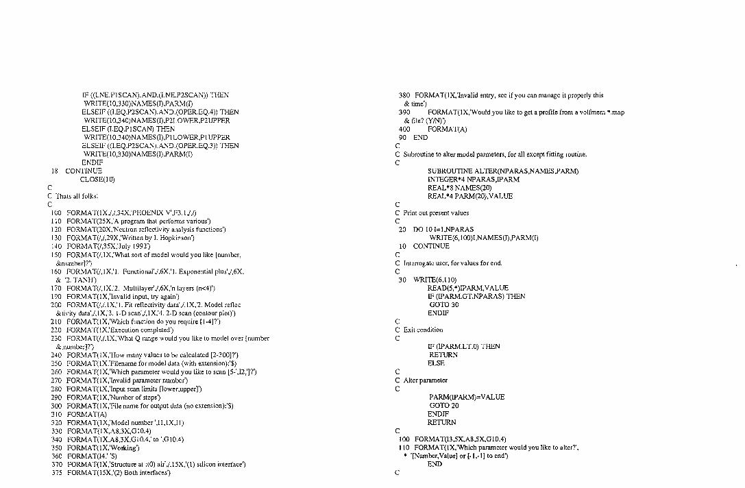
IF ((I.NE.PISCAN).AND.(1.NE.P2SCAN)) THEN WRITE(l0,330)NA!v1ES(I),PARM(I)
ELSEIF ((I.EQ.P2SCAN).AND.(OPER.EQ.4)) THEN WRITE(l0.340)NAN1ES(I),P2LOWER,P2UPPER
ELSEIF (l.EQ.P!SCAJ\') THEN WRITE(l0,340)NA!v1ES(l).Pl LOWER,Pl UPPER
ELSEIF ((l.EQ.P2SCAN).AND.(OPER.EQ.3)) THEN WRITE (I 0,3 30)NAl'viES(l).P ARM(!)
ENDIF 18 CONTINUE
CLOSE(IO) c C Tnats all folks! c
I 00 FORMA T(l X./,/,34X,'PHOENIX V' .F3. 1./.{) II 0 FORMA T(25X,' A program that perfonns various') 120 FORMAT(20X,'Neutron reflectivity analysis functions') 130 FORMAT(I,/,29X,'Written by I. Hopkinson') 140 FORMA T(/,35X,'July 1992') !50 FORMA T(/.IX,'What sort of model would you like [number,
&number]'?') 160 FORMAT(/,1X,'i. Functionai'./.6X,'i. Exponential plus',/,6X,
& '2. TANH') 170 FORMAT(/.IX,'2. Multilayer'./,6X,'nlayers (n<4)') 190 FORMA T(IX,'lnvalid input, try again') 200 FORMAT(/,/,lX,'i. Fit reflectivity data',/,IX,'2. Model reflec
&tivity data',/,IX,'3. 1-D scan',/,IX,'4. 2-D scan (contour plot)') 210 FORMAT(lX,'Which function do you require [ 1-4]?') 220 FORMAT(lX,'Execution completed") 230 FORMA T(/,/,lX,'What Q range would you like to model over [number
&,nun1ber]?') 240 FORMAT(JX,'How many values to be calculated [2-300]?') 250 FORMA T(IX,'Filename for model data (with extension):'$) 260 FORMA T(l X,'Which parameter would you like to scan [5-'.!2,']?') 270 FORMA T(lX,'Invalid parameter number') 280 FORMA T(lX,'Input scan limits [lower,upper]') 290 FORMA T(lX,'Number of steps') 300 FORMA T(l X,'File name for output data (no extension):'$) 310 FORMAT(A) 320 FORMA T(IX,'Model number ',11, LX,Il) 330 FORMA T(l X,A8,3X,G 10.4) 340 FORMA T(IX,A8,3X,G 10.4,' to '.G l 0.4) 350 FORMAT(lX,'Working') 360 FORMAT(I4,' '$) 370 FORMAT(IX,'Structure at :(0) air'./,15X,'(l) silicon interface') 375 FORMAT(15X,'(2) Both interfaces')
380 FORMAT(IX,'Invalid entry, see if you can manage it properly this &time)
390 FORMAT(IX,'Would you like to get a profile from a volfmem *.map & file? (YIN)')
400 FORMA T(A) 90 END
c C Subroutine to alter model panneters, for all except fitting routine. c
c
SUBROUTINE ALTER(NPARAS,NANIES,PARM) INTEGER*4 NPARAS,IPARM REAL*8 NAN1ES(20) REAL*4 PARM(20),VALUE
C Print out present values c
20 DO 10 l=I,NPARAS WRITE(6,IOO)I,NAMES(I),PARM(l)
10 CONTINUE c C Interrogate user, for values for end c
30 WRITE(6,1!0)
c
READ(5, *)IP ARM,V AL UE IF (IPARM.GT.NPARAS) THEN GOT030
END IF
C Exit condition c
c
IF (IPARM.LT.O) THEN RETURN
ELSE
C Alter parameter c
c
PARM(IPARM)=VALUE GOT020
END IF RETURN
100 FORMA T(I3,5X,A8,5X,G!0.4) I 10 FORMAT(! X, 'Which parameter would you like to alter?',
* '[Number, Value] or [-1,-1] to end') END
c

c C Subroutine to REA DIN data c
c
SUBROUTINE READIN(NFIT,XUSE,YUSE,YRUSE,TEXT) REAL XUSE(300),YUSE(300),YRUSE(300),DUM INTEGER NFITJN LOGICAL EXISTS CHARACTER FILNAM*30,TRIPE*3,DUM1 * 12,DUM2*80
C Get fil~name and identify extension c
c
10 WRITE(6,!00) READ(S,!!O)FILNAM INQUIRE(FILE=FILNAM,EXIST=EXISTS) IF (.NOT.EXISTS) THEN WRITE(6,120) GOTO 10
ENDIF IN=INDEX(Fll..NAM,' ') TRIPE=FILNAM((IN-3):(IN-l))
C Read .DRY format (number of points, followed by x y pairs. followed by C title). Fractional error is calculated and placed in YRUSE c
c
IF ((TRIPE.EQ.'DRY').OR.(TRIPE.EQ.'dry')) THEN OPEN(UNIT=10,FILE=FILNAM,STATUS='OLD') READ(lO,*)NFIT NFIT=NFIT-4 DO 20 I=l,NFIT READ(IO,*)XUSE(I).YUSE(I), YRUSE(l)
IF (YUSE(I).LE.O.O) THEN YUSE(l)= I O**YUSE(l-1) YRUSE(1)=YUSE(l-l)*YRUSE(l-l)
END IF c
. TEMP=1'RUSE(l)/YUSE()) YRUSE(I)=TEMP YUSE(I)=LOG IO(YUSE(l))
20 CONTINUE
c
READ(! 0, 130)TEXT CLOSE(IO)
C Read .DEY format (the VOLFMEM format) c
ELSEIF ((TRIPE.EQ.'DEV').OR.(TRIPE.EQ.'dev')) THEN
OPEN(UNIT=l O,FILE=FILNAM,ST A TUS='OLD') READ(! 0, 130) TEXT READ(l0,130)DUM2 READ(10,*,END=SO)(XUSE(I),YUSE(I),YRUSE(I),DUM,I=1,1000)
50 NFIT=l-1 c
DO 60 l=l,NFIT IF (YUSE(I).LE.O.O) THEN YUSE(l)=IO**YUSE(l-1) YRUSE(l)=YUSE(l-I)*YRUSE(l-1)
END IF TEMP= YR USE(l)/YUSE(l) YRUSE(I)=TEMP YUSE(l)=LOG IO(YUSE(l))
60 CONTINUE CLOSE(IO)
c C Read .DA T format (the CRISP ASCII format) C Fractional error is calculated and placed in YRUSE c
ELSEIF ((TRIPE.EQ.'DA T).OR.(TRIPE.EQ.'dat')) THEN OPEN(UNIT=IO,FILE=FILNAM,STATUS='OLD') READ(10,150)DUMl,NFIT READ(IO,IIO)DUM2 READ(10,110)DUM2 READ(10,1IO)DUM2 NFIT=NFIT-1 DO 30 l=I,NFIT READ(10, *)XUSE(I),YUSE(I), YRUSE(l) TEMP=YRUSE(I)/YUSE(l) YR USE(!)= TEMP YUSE(l)=LOG IO(YUSE(l))
30 CONTINUE READ(lO,*)XUSE(NFIT+l),YUSE(NFIT+l),YRUSE(NFIT+1) READ(l0,1IO)TEXT CLOSE(IO)
ELSE WRITE(6,140) GOTO 10
END IF c C Histogram format conversion c
NFIT =NFIT -1 DO 40 I=l,NFIT XUSE(l)=(XUSE(l)+XUSE(l+ 1))/2
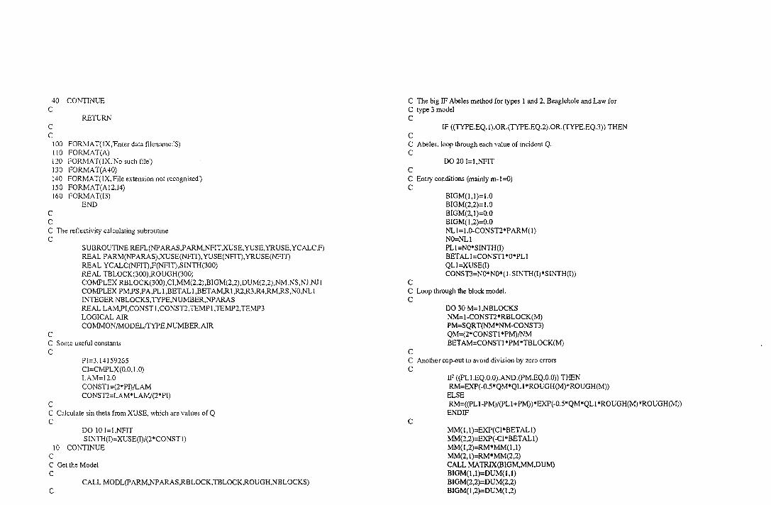
40 CONTINUE c
c c
RETURN
100 FORMAT(IX,'Enter data filename:'$) 110 FORJV!AT(A) 120 FORMAT(IX,'No such file') 130 FORMAT(A40) 140 FORMAT(IX,'File extension not recognised') 150 FORMAT(A12,!4) 160 FORMAT(l3)
c c
END
C 'TI1e reflectivity calculating subroutine c
c
SUBROUTINE REFL(NP ARAS,P ARM,NFIT ,XUSE, YUSE,YRUSE, YCALC.F) REAL PARM(NP ARAS),XUSE(NFIT). YUSE(NFIT), YRUSE(NFIT) REAL YCALC(NFIT) ,F(NFIT) ,S INTH(300) REAL TBLOCK(300),ROUGH(300) COMPLEX RBLOCK(300),Cl,MM(2,2) ,BI GM(2,2),DUM(2,2),NM .N S ,N J .NJ I COMPLEX PM,PS,PA,PL1,BETAL1,BETAM,RI,R2,R3,R4,RM,RS,NO,NLI INTEGER NBLOCKS,TYPE,NUMBER,NP ARAS REAL LAM,PI,CONSTI ,CONST2,TEMP l.TEMP2,TEMP3 LOGICAL AIR COMN!ON!MODEL!TYPE,NUMBER.AIR
C Some useful constants c
c
?1=3.14159265 CI=C.tv!PLX(O.O, 1.0) LAM=12.0 CONST1=(2*PI)!LAM CONST2=LAM*LAM/(2*PI)
C Calculate sin theta from XUSE, which are values of Q c
DO 10 l=l.NFIT SINTH(I)=XUSE(I)/(2*CONSTI)
10 CONTINUE c C Get the Model c
CALL MODL(P ARM,NP ARAS,RBLOCK,TBLOCK.ROUGH.NBLOCKS) c
C The big IF Abeles method for types I and 2, Beaglehole and Law for C type 3 model c
IF ((TYPE.EQ.I).OR.(TYPE.EQ.2).0R.(fYPE.EQ.3)) THEN c C Abeles, loop through each value of incident Q. c
DO 20 l=l,NFIT c C Entry conditions (mainly m-1=0) c
c
BIGM(I,I)=I.O BIGM(2,2)=1.0 BIGM(2,1)=0.0 BIGM(l,2)=0.0 NL1=1.0-CONST2*PARM(I) NO=NL! PLI=NO*SINTH(l) BETALI=CONST1 *O*PLI QLI =XUSE(I) CONSTI=NO*NO*(I-SINTH(l)*SINTH(I))
C Loop through the block model. c
c
DO 30 M=l,NBLOCKS NM=1-CONST2*RBLOCK(M) PM=SQRT(NM*NM-CONSTI) QM=(2*CONST!*PM)/NM BETAM=CONSTI *PM*TBLOCK(M)
C Another cop-out to avoid division by zero errors c
c
IF ((PLI.EQ.O.O).AND.(PM.EQ.O.O)) THEN RM=EXP(-0.5*QM*QL 1 *ROUGH(M)*ROUGH(M))
ELSE RM=((PL 1-PM)/(PL I +PM) )*EXP(-0.5*QM*QL 1 *RO UGH(M)*ROUGH(M)) END IF
MM(l,1)=EXP(CI*BETAL1) MM(2,2)=EXP(-CI*BETAL1) MM(l,2)=RM*MM(I,l) MM(2, I)=RM*MM(2,2) CALL MA TRIX(BIGM,MM,DUM) BIGM(I,l)=DUM(l,l) BIGM(2,2)=DUM(2,2) BIGM(I,2)=DUM(l,2)

BIGM(2,I)=DUM(2,I) BETALI=BETAM QLI=QM PLI=PM
30 CONTINUE c C Exit calculations including calculating R for I value of Q c
c
NS=I-CONST2*PARM(2) PS=SQRT(NS*NS-CONST3) QS=2*CONSTI *PS/NS RS=((PL 1-PS)/(PL I +PS))*EXP( -0.5*QL I *QS*(ROUGH(NBLOCKS+ I )**2)) MM(1.I)=EXP(Cl*BETALI) MM(2,2)=EXP(-CI*BET ALI) MM( 1.2)=RS*tviM(I , 1) MM(2. I)=RS*MM(2,2) CALL MATRIX(BIGM,MM,DUM) BIGM(1,1)=DUM(l,1) BIGM(2. l)=DUM(2. I) BIGM(2.2)=DUM(2.2) BIGM(l ,2)=DUM(I,2) TEMPI=BIGM(2.1)*CONJG(BIGM(2,1)) TEMP2=BIGM( 1,l)*CONJG(BIGM(l,1))
C 'This bit is a fiddle, because for some reason with functional fom1 models C temp I=temp2=0. This fiddle allows the program to run and doesn't seem C to grossly effect the profiles generated. c
c
IF ((TEMP2.EQ.O.O).AND.(TEMP1.EQ.O.O)) THEN TEMPI=! TEI'v1P2=1 ENDIF
YCALC(I)=LOG 10(TEI'vll' I/TEI'vll'2) 20 CONTINUE
ENDIF c C Call the resolution routine c
CALL RESL(XUSE.YCALC,P ARM.NP ARAS,NFID c C Calculate the residual F, this is where error weighting code should C be inserted. Done- note READIN has also been altered to make 'l.'RUSE(i) C the fractional error in Y. c
DO 60 I=I.NFIT
F(I)=(YUSE(l)-YCALC(I))!YRUSE(I) 60 CONTINUE
c C The End c
c
RETURN END
C Matrix multiplication routine c
c c
SUBROUTINE MA TRIX(A,B.C) COMPLEX A(2,2),B(2,2),C(2,2) C(1, l)=A( 1, 1)* B( 1,1 )+A (I ,2)*8(2,1) C(l,2)=A(l, 1)*B(l ,2)+A(l ,2)*B(2,2) C(2,l)=A(2, I)*B(1,1)+A(2,2)*B(2,1) C(2,2)=A(2, 1 )*B(I ,2)+ A(2,2)*B(2,2) RETURN END
C The resolution effect routine, this is a modification of the routine C used previously. c
c
SUBROUTINE RESL(XUSE, YCALC,P ARM,NP ARAS.NFIT) REAL XMIN,XMAX, YCALC(NFIT),XUSE(NFIT).PARM(NPARAS) REAL RESULT, YTEMP(300),TEMP,YMIN ,YMAX INTEGER START .END
C Return without doing anything if resolution=O%- otherwise C you get a division by zero error c
c
IF (PAR.t'v1(5).EQ.O.O) THEN RETURN
END IF
C Main loop through all the points c
c
DO 10 l=l,NFIT XMIN=XUSE(I)-(P ARM(S)/1 OO.O)*XUSE(I) XMAX=XUSE(I)+(P ARM(S)/1 OO.O)*XUSE(I)
C Test for beginning or end of 'point' integral lying outside dataset C then do loop to identify range of integral c
IF (XMAX.GT.XUSE(NFID) THEN END=NFIT+I

END IF IF (XMIN.LT.XUSE(I)) THEN START=O
ENDIF DO 20 J=l.NFIT-1 IF ((XUSE(J).LE.XMIN).AND.(XUSE(J+l).GT.XMIN)) TI-IEN START=l
ENDIF IF ((XUSE(J).GT.XMAX).AND.(XUSE(J- I).LE.XMAX)) THEN END=J-1
ENDIF 20 CONTINUE
c C Bit to wo1k out first part of integral c
c
RESULT=O.O IF (XMIN.GT.XUSE(l)) T!-IEN TEMP=(XMIN-XUSE(ST ART))/(XUSE(ST ART+ 1)-XUSE(ST ART))
. YrvliN= YCALC(ST ART)+(YCALC(ST ART+ 1)-YCALC(START))*TEtv!P RESUL T=RESUL T +O.S*(YMIN+ YCALC(START + l))*(XUSE(START + 1)-XMIN)
END IF
C Main part of integral c
DO 30 J=START + l,END-2 RESUL T=RESUL T +O.S*(YCALC(J)+ YCALC(J+ I))*(XUSE(J+ 1)-XUSE(J))
30 CONTINUE c C End part of integral c
IF (END.EQ.(NFIT+l)) THEN RESUL T=RESUL T +(YCALC(NFIT))*(XMAX-XUSE(NFIT)) ELSE TEMP=(XMAX-XUSE(END-1 ))/(XUSE(END)-XUSE(END-1 )) YMAX= YCALC(END-1)-(YCALC(END-1)-YCALC(END))*TEMP RESUL T=RESULT +0.5*(YMAX+ YCALC(END-l))*(XMAX-XUSE(END-1))
END IF RESULT=RESUL T/(XMAX-XMIN) YTEMP(f)=RESUL T
10 CONTINUE c C Transfer integral back to YCALC c
DO 40 l=l.NFIT YCALC(l)= YTEtv!P(I) YTEMP(l)=O.O
40 CONTINUE RETURN END
c c C MODL routine to set up model for REFL. c
c
SUBROUTINE MODL(P ARM.NPARAS,RBLOCK, TBLOCK,ROUGH.NBLOCKS) INTEGER TYPE,NUMBER,NBLOCKS,AIR,N COMMON/MODEL!lYPE,NUMBER,AIR COMPLEX RBLOCK(300) REAL PARM(NPARAS),TBLOCK(300),ROUGJ-1(300) REAL BSIZE,Z,TEMP,TEMP2,TEMP3,TEMP4,TEMPS,TOL,UPPERI,UPPER2 LOGICAL EXISTS CHARACTER*30 MAPFILE
C lbis is the New Model functional form profile routine. It takes the C block size as a user input, there is no safety check to make sure the C program can handle the required number of blocks - so ensure that C thick/bsize<300 for safety. Profiles can be fitted at the air either/and C the silicon interface. Exponential plus or TANH profiles are supported c
c
IF (TYPE.EQ.I) THEN BSIZE=PARM(6) ROUGH(l)=PARM(8) TOL=O.OI UPPERI=O UPPER2=0 TEMP3=PARM(I I)-PARM(7)
TEMP4=PARM(l4)-PARM(7)
C l11is part works out the upper bounds for the profiles C its quite impottant because on the basis of these results various things C are or are not calculated c
IF (NUMBER.EQ.l) THEN IF ((AIR.EQ.O).OR.(AIR.EQ.2).AND.(TOL.L T.TEMP3)) THEN UPPERI=PARM(I3)*(LOG(TEMP3n·oL)**(l/PARM(l2)))
END IF IF ((AlR.EQ.l).OR.(AlR.EQ.2).AND.(TOL.L T.TEMP4)) Tl-IEN UPPER2=PARM(I6)*(LOG(TEMP4/TOL)**(l/PARM(l5)))
END IF ELSEIF (NUMBER.EQ.2) THEN IF ((AIR...EQ.O).OR.(AIR.EQ.2).AND.(TOL.L T.TEMP3)) THEN UPPERI=PARM(l2)-PARM(l3)*(!.34*(-1+2*TOL/TEMP3))/2
c
c
ENDIF IF ((AIR.EQ.l).OR.(AIR.EQ.2).AND.(TOL.L T.TEMP4)) THEN UPPER2=PARM(l5)-PARM(l6)*(1.34*(-1+2*TOL!TEMP4))/2
ENDIF ENDIF
UPPERI=INT(UPPERI!BSIZE)*BSIZE UPPER2=INT(UPPER2(13SIZE)*BSIZE
C This next bit actually calculates the profile - the bulk block C the two interfaces as necessal)'- if upper! +upper2> thickness C then there is no need to calculate the bulk block c
c
IF ((UPPER!+UPPER2).LT.PARM(6)) THEN NBLOCKS=(UPPER I /BSIZE)+ (UPPER2/BSIZE)+ l
C Calculating the bulk block c
c
IF (UPPER!.EQ.O) THEN N=l
ELSE N=(UPPER I /BSIZE)+ I
END!F TEMP2=PARM(4)*PARM(7)+PARM(3)*(l-PARM(7)) TBLOCK(N)=P ARM( l 0)-UPPER!-UPPER2 RBLOCK(N)=CMPLX(TEMP2,0.0)
C This bit calculates the Air interface profile c
IF (UPPERI.GT.O) THEN DO 10 l=l,(UPPERI/BSIZE) TBLOCK(l)=BSIZE Z=(l-1 )* BSIZE+ BSIZE/2 IF (NUMBER.EQ.l) THEN TEMP2=TEMP3*EXP(-(Z!PARM(I3))**PARM(I2))
ELSE TEMP2= TEMP3*(1 + T ANH(2*(P ARM( 12)-Z)!P ARM( 13)))/2
END IF TE!YIP2=(PARM(7)+ TE!v!P2)*P ARM(4)+(P ARM(7)+ TEMP2-l)*PARM(3) RBLOCK(l)=CMPLX(TEMP2.0.0)
10 CONTINUE END!F
c C This is the silicon interface part c
IF (UPPER2.GT.O) THEN
DO 20 l=l,(UPPER2/BSIZE) TBLOCK(N+l)=BSIZE Z=UPPERI+(PARM(IO)-UPPER2)+(1-l)*BSIZE+BSIZE/2 IF (NUMBER.EQ.l) THEN TEMP2=TEMP4*EXP(-((PARM(IO)-Z)/PARM(I6))**PARM(l5))
ELSE TEMP2=TEMP4*(1-TANH(2*((PARM(JO)-PARM(l5))-Z)!PARM(l6)))/2
END IF TEMP2=(PARM(7)+ TEMP2)*PARM(4)+(PARM(7)+ TEMP2-l )*PARM(3) RBLOCK(l)=CMPLX(TEMP2,0.0)
20 CONTINUE END!F
c C This is what to do if there is no block in the middle c
ELSE NBLOCKS=INT(P ARM(l 0)/BSIZE)
DO 30 I=I,INT(PARM(lO)/BSIZE) TBLOCK(l)=BSIZE Z=(l-l)*BSIZE+BSIZE/2 IF (NUMBER.EQ.l) THEN TEMP2=TEMP3*EXP(-(Z/PARM(l3))**PARM(l2)) TEMP=TEMP4*EXP(-((PARM(l0)-Z)!PARM(l6))**PARM(l5))
ELSE TEMP2=TEMP3*(l+TANH(2*(PARM(I2)-Z)!PARM(l3)))/2 TEMP=TEMP4*(l-TANH(2*((PARM(l0)-PARM(I5))-Z)!PARM(l6)))/2 END IF TEMPS=P ARM(7)+ TEMP2+ TEMP TEMPS=TEMPS*PARM(4)+(1-TEMP5)*PARM(3) RBLOCK(l)=CMPLX(TEMPS,O.O)
30 CONTINUE END!F
C This sticks an Si02 layer in c
c
c
NBLOCKS=NBLOCKS+ I TBLOCK(NBLOCKS)=IS.O RBLOCK(NBLOCKS)=CMPLX(3.676E-6,0.0) ROUGH(NBLOCKS)=PARM(9)
ROUGH(NBLOCKS+ 1)=5.0
RETURN END!F
C Block model c
IF (TYPE.EQ.2) THEN

NBLOCKS=NUMBER ROUGH(l)=PARM(6) TEMP3=PARM(5+NUMBER*3) DO 40 l=l,NUMBER TBLOCK(I)=P ARM(5+1*3) ROUGH(I+I)=PARM(6+1*3) TEMP=PARM(4+1*3)*PARM(4)+(1-PAR1vi(4+1*3))*PARM(3) RBLOCK(I)=CMPLX(TEMP,O.O) TEMP3= TEMP3-P ARM(5+1*3)
-lO CONTINUE TEMP3= TEMP3+PARM(5+NUMBER *3)
C Modification to vary blocks independantly, temp3 is ignored C TBLOCK(NUMBER)=TEW3
RETURN END IF
c C Read in a* .map file from volfmem, this should only occur for the C 'Model reflectivity' option. c
50
60 70
80
100 110 120
IF (TYPE.EQ.3) THEN WRITE(6,!00) READ(S,l IO)MAPFILE IN QUIRE(FILE=MAPFILE,EXIST =EXISTS) IF (.NOT.EXISTS) THEN WRITE(6,120) GOTOSO
ENDIF OPEN(UNIT=IO,FILE=MAPFILE,STATUS='OLD') DO 60 1=1,300 READ(lO,*.END=70)TBLOCK(I),TE1vlP,TEMP2 RBLOCK(l)=CMPLX(TEMP*PARM(4)+(1-TEtvlP)*P ARl\-1(3),0.0) CONTINUE NBLOCKS=l- I DO SO 1=1 ,NBLOCKS- I TBLOCK(I)=TBLOCK(l+l)-TBLOCK(I) CONTINUE TBLOCK(NBLOCKS)=TBLOCK(NBLOCKS-1) RETURN
ENDIF FORMAT(lX,'Enter volfmem output filename:'$) FORMAT(A) FORMAT(IX,'No file by that name, have another go.') END
WELDER
c C WELDER is a program that combines CRISP datasets, the datasets must be C rebinned to the same spacing and normalisation factors should have been C applied. Negative values for the reflectivity are replaced by the C error in the reflectivity and the number of such replacements is recorded C !.H. 11/l/93 c
c
PROGRAM WELDER CHARACTER DUM 1 *26,DUM2(8)*80,FILEN AM*20 INTEGER NFIT,I,ERR REAL XI (300), YI (300),YEI (300),X2(300),Y2(300),YE2(300) REAL X(300),Y(300),YE(300) LOGICAL FLAG I ,FLAG2,EXISTS
C Load in datasets to be combined- at present it is assumed that they are C called templ.dat and temp2.dat c
OPEN (UNIT=IO,FILE='TEMPI.DAT,STATUS='OLD') c C Header I c
DO 10 1=1,6 READ (IO,lOO)DUM2(l)
lO CONTINUE
c C Datal c
READ(IO,liO)DUMl,NFIT READ(IO,IOO)DUM2(7) READ(! 0, I OO)DUM2(8)
DO 20 I=I,NFIT READ(! O,*)XI (!), Y1 (l),YE 1 (I)
20 CONTINUE CLOSE(IO)
c C Second dataset c
OPEN (UNIT=IO,FILE='TEMP2.DAT,STATUS='OLD') c C Header2 c
DO 30 1=1,6 READ (10,100)DUM2(1)
30 CONTINUE

c C Data 2 c
READ(10,1!0)DUM1,NFIT READ(10,100)DUM2(7) READ(IO,lOO)DUM2(8)
DO 40 l=l,NF!T READ( I 0. *)X2(!). Y2(l). YE2(!)
40 CONTINUE CLOSE(IO)
c C Setup combine loop c
c
FLAG1=.TRUE. FLAG2=.FALSE.
C St,\ltloop c
DO 50 1=1,NFIT IF ((YI (I).EQ.O.O).AND.(YE I (I).EQ.O.O)) THEN FLAG I =.FALSE.
END IF IF (FLAGI.AND.FLAG2) THEN X(I)=X1(1) Y(I)=(Y1 (I)+ Y2(I))/2 YE(I)=(YE1 (!)+ YE2(1))!2
ENDIF IF (FLAG!.AND.(.NOT.FLAG2)) THEN X(I)=XI(I) Y(I)=YI(I) YE(I)= YE I (I)
END IF IF ((.NOT.FLAGI).AND.FLAG2) Tl-IEN X(I)=X2(1) Y(I)=Y2(1) YE(l)=YE2(l)
ENDIF IF ((Y2(I).NE.O.Q).AND.(YE2(l).NE.O.O)) THEN FLAG2=.TRUE.
END IF 50 CONTINUE
c C Data is now written out in the *.dry fom1at c
WRITE(6,120) READ(5,100)FILENAM
c
OPEN (UNIT=10,FILE=FILENAM,STATUS='NEW) WRITE(IO,*)NFIT ERR=O DO 60 I=1,NFIT
C This IF statement traps any negative values for the reflectivity c
c 60
IF (Y(l).L T.O.O) THEN WRITE(! O,*)X(l), YE(fJ, YE(I) ERR=ERR+l
ELSE WRITE(IO.*)X(l),Y(I).YE(I)
END IF
CONTINUE WRITE(IO,I30)DUM2(I) CLOSE(IO) WRITE(6,140)ERR
I 00 FORMA T(A) II 0 FORMA T(A26,14) 120 FORMA T(l X,' Enter name for combined file:'$) 130 FORMAT(A40) 140 FORMAT(IX,I4,' negative reflectivity values replaced')
END
lBAN'f AM (cllata fiUed as I(Q) vs Q)
c C BANTAM is a program that calculates chi from SANS data C as well as radii of gyration. (via the Kuhn length, a) C W!itten to process d-PS/h-PS standard data, NH=ND and RGH=RGD C are forced because d-PS and h-PS had identical molecular weights C See de Gennes p261,p109 and refs 76,84. C I. Hopkinson 1/10/92 c
PROGRAM CHICKEN EXTERNAL READIN,SCA TTER COMMON!TITLES/NAMES(20),TX(5),TY(5),NPARAS COMMON/WORK/W(3066) COMMON/IO/INITY,IOUTTY DOUBLE PRECISION NAMES DATA NAMES/Chi ','phi(d) ','Rg(h)/A ','Rg(d)/A ','N(d)
& 'N(h) ','V ','b(h) ','b(d) ','Instrum ·•
& 10*' '/ DATA TX/Q/A'''.'-1 ',3*' 'I DATA TY!l(Q)','/CM"','-1 ',2*' '/ DATA PNAM(SHED'/ VERP=l.O INTTY=5 IOUTIY=6 NPARAS=IO
, WRITE(6,100) WRITE(6,1 I 0) WRITE(6,120) CALL FI1FUN(PNAM,READIN,SCA TTER) CALL FINITI(0,750)
I 00 FORMAT(1X./././,36X,'CHICKEN'./././) II 0 FORMA T(l X,25X,' A program to fit SANS data',/,/,/) 120 FORMAT(1X,25X,'By Ian Hopkinson (1/10/92)'./././)
END c C REA DIN data from LOQ c
SUBROUTINE READIN(l'<'FIT .XUSE,YUSE.YRUSE,TEXT) REAL*4 XUSE(300),YUSE(300),YRUSE(300) INTEGER NFIT.I,J LOGICAL EXISTS CHARACTER FILNAM*60,DUMMY*80
10 WRJTE(6,100) READ(5, 110)FILNAM INQ UIRE(FILE=FILNAM,EXIST=EXISTS) IF (.NOT.EXISTS) THEN WRITE(6.120) GOTO 10
END IF OPEN (UNIT =I O,FILE=FILN AM.ST A TUS='OLD') DO 20 1=1,5 READ(! 0,130)DUMMY
20 CONTINUE DO 30 1=1.300 READ(IO.* .END=40)XUSE(f),YUSE(I),YRUSE(I) YRUSE(I)=YRUSE(I)/YUSE(l)
30 CONTINUE 40
100 110 120
Nf!T=I-1 CLOSE(!O) RETURN FORMA T(IX,'Enter filename:'$) FORMAT(A) FORMA T(IX,'File does not exist')
c
130 FORMA T(A) END
C Calculation routine c
c
SUBROUTINE SCA TIER(NP ARAS,P ARM,NFIT ,XUSE, YUSE,YRUSE, YCALC.F) REAL*4 PARM(NPARAS),YCALC(NFIT),YRUSE(NFIT),YUSE(NFIT) REAL *4 XUSE(NFIT),S(300),F(NFIT) REAL*4 PREFACTOR,RGH,RGD,PHI,CHI,ND,NH,GDH,GDD DO 10 l=l,NFIT PREFACTOR=(PARM(8)-PARM(9))*(PARM(8)-PARM(9))/PARM(7) ND=PARM(5) NH=ND RGD=PARM(4) RGH=RGD PARM(3)=RGH PHI=PARM(2) CHI=PARM(l) GDH=GD(RGD,XUSE(l)) GDD=GD(RGH,XUSE(l)) TEMPl=l.O/(ND*PHI*GDH) TEMP2=1.0/(NH*(l-PHI)*GDD) YCALC(l)=PARM(IO)*PREFACTOR/(TEMPI+TEMP2-2*CHI) F(l)=(YCALC(l)-YUSE(l))/YRUSE(l)
10 CONTINUE RETURN END
C Debye Fw1ction. gd. c
REAL FUNCTION GD(RG,Q) REAL RG,Q,TEMP
. TEMP=RG*RG*Q*Q GD=2*(TEMP+EXP(-TEMP)-l)/(TEMP*TEMP) END
IPUJLJLJE1'3
c C PULLET is a program that calculates chi and radii of gyration C from SANS data. Unlike CHICKEN displays fits and data in the Kratky C format. C See de Gennes p26l,pl09 and refs 76,84. C I. Hopkinson 1/10/92

C Modified 16/2/93- seemed to have GOD, GDH mixed up -panic over C TEl'v!PI and TEMP2 were mixed up, reversing the effect of GDD and GDH being C mixed. C 23/8/93- Modified to look at 'asymmetric' blends such as PEO/PMMA C see ref I 13 C 12/I 0/93 : Modified to look at polydisperse blends such as isotactic PMMA C see ref Il3 c
c
PROGRAM PULLET EXTERNAL READIN,SCA TTER COMMON/TITLES/NArviES(20),TX(5),TY(5),NPARAS COMMON/WORK./W(3066) COMMON/10/!NTTY,IOUTTY DOUBLE PRECISION NAMES DATA NAMES/Chi ','phi(d) ','Rg(h)/A ','Rg(d)/A ',
& 'N(u) ','N(l1) ','DP(d) ','DP(h) ' & 'Vh ','Vd ','b(h) ', & 'b(d) ','Instrum '. & 7*' '/
DATA TX!Q/A"','-I ',3*' '/ DATA TI'/I(Q)','/CM"','-1 '2*' '/ DATA PNAM/SHED'/ VERP=I.O INTTY=5 IOUTTY=6 NPARAS=!3 WRITE(6,1 00) WRITE(6,1!0) WRITE(6,120) CALL FITFUN(PNAM,READIN,SCA TIER) CALL FINITT(0,750)
100 FORMAT(lX,/,/./.21X,'PULLET3- Asymmetry, Polydispersity'./,/,1) 110 FORMAT(IX,25X,'A program to fit SANS data',/,/,/) 120 FORMAT(IX,25X,'By Ian Hopkinson (1/10/92)',/,/,/)
END
C READ IN data from LOQ c
SUBROUTINE READ IN (NFIT,XUSE, YUSE, YRUSE,TEXT) REAL *4 XUSE(300), YUSE(300), YRUSE(300) INTEGER NFIT,I,J LOGICAL EXISTS CHARACTER FILNAM*60,DUMMY*80
10 WRITE(6,100) READ(5,110)FILNAM IN QUIRE(FILE=FILN AM,EXIST =EXISTS)
IF (.NOT.EXISTS) THEN WRITE(6,120) GOTO 10
END IF OPEN (UNIT=10,FILE=FILNAM,STATUS='OLD') DO 20J=1,5 READ(IO,l30)DUMMY
20 CONTINUE DO 30 1=1,300 READ(! 0, * ,END=40)XUSE(I),YUSE(I), YRUSE(I) YR USE (I)= YRUSE(I)/YUSE(I) YUSE(I)= YUSE(I)*XUSE(l)*XUSE(I)
30 CONTINUE 40 NFIT=l-1
c
CLOSE(!O) RETURN
I 00 FORMAT(!X,'Enter filename:'$) II 0 FORMA T(A) 120 FORMA T(lX,'File does not exist') 130 FORMA T(A)
END
C Calculation routine c
SUBROUTINE SCA TTER(NP ARAS,P ARM,NFIT,XUSE,YUSE, YRUSE, YCALC,F) REAL*4 PARM(NPARAS),YCALC(NFID.YRUSE(NF!D,YUSE(NFID REAL *4 XUSE(NFID,S(300),F(NFID REAL*4 PREFACTOR,RGH,RGD,PHI,CHI,ND,NH,GDH,GDD REAL*4 DPD,DPH REAL*4 VH,VD,VO,NA NA=6.022E23 DO 10 I=I,NFIT ND=PARM(5) NH=PARM(6) DPD=PARM(7) DPH=PARM(S) VH=PARM(9) VD=PARM(IO) RGD=PARM(4) RGH=PARM(3) PHI=P ARM(2) CHI=PARM(l) VO=l/((PHI/VD)+(l-PHI)!VH) PREFACTOR=VO*((P ARM(!! )!VH-P ARM(I2)/VD)**2)
c C APPEARED TO HAVE THESE TWO MIXED UP PREVIOUSLY
C TI-!IS IS WHERE POL YDJSPERSITY CO RECTI ON GOES IN c
c
GDH=GD(RGH,DPH,XUSE(f)) GDD=GD(RGD,DPD,XUSE(I))
IF (.NOT.(RGH.EQ.O.OR.RGD.EQ.O)) THEN TE!:v!P I =VO/(ND*PHI*GDD*VD)
TEMP2=VO/(NH*(I-PHI)*GDH*VH) END IF YCALC(f)=P ARM(l3)*PREF A CTOR!(TEl:v!P I+ TEl:v!P2-2*CHI) YCALC(l)=YCALC(I)*XUSE(I)*XUSE(I) F(I)=(YCALC(I)-YUSE(I))!YRUSE(I)
10 CONTINUE
c
RETURN END
C Debye Function, gd. C Dcbye. function modified to allow polydispersity (12/1 0/93) c
REAL*4 FUNCTION GD(JW,DP,Q) REAL*4 RG,Q,TEtv!P,DP,HI TEl:v!P=RG*RG*Q*Q HI=I/(DP-1) GD=2*((Hl/(Hl+TEl:v!P))**HI-l + TEMP)/(TEl:v!P*TEl:v!P) END
1Pullet4 (lPullllet a~rndllPu.nllllet2 snmplle cases of lPulllet4)
c C PULLET is a program that calculates chi and radii of gyration C from SANS data. Unlike CHICKEN displays fits and data in the Kratky C fonnat. C See de Gennes p261 ,pI 09 and refs 76,84. C I. 1-!opl:inson Ill 0/92 C Modified 16/2/93- seemed to have GOD, GDH mixed up -panic over C TE!:v!PI :UJd TEMP2 were mixed up, reversing the effect of GOD and GDH being C mixed. C 23/8/93 - Modified to look at 'asymmetric' blends such as PEO/PMMA C see ref 113 C !8/5/94 - Modified to fit a flat background c
PROGRAM PULLET EXTERNAL READIN,SCA TTER COMMON/TITLES/NAMES(20).TX(5).TY(5).NPARAS
c
COMMON/WORK!W(3066) COMMON/IO!INTTY,JOUTTY DOUBLE PRECISION NAMES DATA NAMES/Chi ','phi(d) ','Rg(h)/A ','Rg(d)/A ',
& 'N(d) ','N(h) ','Vh ','Vd ','b(h) ', & 'b( d) ','lnstmm ','Backgrd ', & 8*' '/
DATA TX/Q/A''','-1 '.3*' '/ DATA TY/I(Q)','/CM"','-1 ',2*' 'I DATA PNAM/SHED'/ VERP=!.O INTTY=5 IOUTTY=6 NPARAS=l2 WRJTE(6, 1 00) WRITE(6,110) WRITE(6,120) CALL FITFUN(PNAM,READIN,SCATTER) CALL FINITT(0,750)
100 FORMAT(1X,/,/,/,29X,'PULLET2- Asymmetry'JJ.fJ 110 FORMA T(IX,25X,'A program to fit SANS data',/,/,/) 120 FORMAT(!X,25X,'By Jan Hopkinson (1/10/92)',/,/,/)
END
C READIN data from LOQ c
10
20
SUBROUTINE READ IN (NFIT ,XUSE,YUSE, YRUSE, TEXT) REAL*4 XUSE(300),YUSE(300),YRUSE(300) INTEGER NFIT,I,J LOGICAL EXISTS CHARACTER FILNAM*60,DUMMY*80 WRITE(6, I 00) READ(S.l!O)ALNAM JNQUrRE(ALE=ALNAM,EXIST=EXISTS) rF (.NOT.EXISTS) THEN WRITE(6,120) GOT010
ENDrF OPEN (UNIT=10,FlLE=FILNAM,STATUS='OLD') DO 20J=l.5 READ(! 0, l30)DUMMY
CONTINUE DO 30 1=1,300 READ(! 0, * ,END=40)XUSE(I),YUSE(J), YRUSE(l) YRUSE(l)=YRUSE(I)/YUSE(I) YUSE(l)= YUSE(I)*XUSE(I)*XUSE(I)

30 40
c
100 110 120 130
CONTINUE NFIT=I-1 CLOSE(IO) RETURN FORMAT(IX,'Enter filename:'$) FORMAT(A) FORMA T(lX,'File does not exist) FORMAT(A) END
C Calculation routine c
c
SUBROUTINE SCA TTER(NP ARAS,P ARM,NFIT,XUSE,YUSE, YRUSE, YCALC,F) REAL*4 PARM(NPARAS),YCALC(NFIT),YRUSE(NFIT),YUSE(NFITJ REAL*4 XUSE(NFIT),S(300),F(NFIT) REAL *4 PREFACTOR,RGI-I,RGD,PHI,CHl,ND,NH,GDH,GDD REAL*4 VH,VD,VO,NA NA=6.022E23 DO 10 l=l,NFJT ND=PARM(5) NH=PARM(6) VH=PARM(7) VD=PARM(8) RGD=PARM(4) RGH=PARM(3) PHI=PARM(2) CHI=PAR...I\1(1) VO=l /((PHI/VD)+(I-PHI)!YHJ PREFACTOR=VO*((PARM(9)/VH-PARM(JO)!YD)**2)
C APPEARED TO HAVE THESE TWO MIXED UP PREVJOUSL Y c
c
GDH=GD(RGH,XUSE(I)) GDD=GD(RGD,XUSE(I))
IF (.NOT.(RGH.EQ.O.OR.RGD.EQ.O)) THEN TEMPl=VO/(ND*PHI*GDD*VD)
TEMP2=V0/(NH*(l-PHI)*GDH*VH) END IF YCALC(l)=P ARM(ll)*PREFACTOR/(TEMP I+ TEMP2-2*CHI)+pmm(12) YCALC(1)=YCALC(I)*XUSE(I)*XUSE(I) F(I)=(YCALC(J)-YUSE(J))!YRUSE(J)
10 CONTINUE
c
RETURN END
C Debye Function, gd. c
REAL*4 FUNCTION GD(RG,Q) REAL*4 RG,Q,TEMP TEMP=RG*RG*Q*Q GD=2*(TEMP+EXP(-TEMP)-l)/(TEMP*TEMP) END
·'· !"·,·,- .
.. s .... ~~-
.~~(1.&\.·-
~,.,~·· ,,r~-'":~:-


