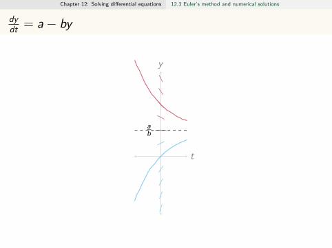
Chapter 12: Solving differential equations 12.3 Euler’s method and numerical solutions

First-Order Linear Differential Equation

dy

dt= a− by

with y(0) = y0 given.

Steady state solutions:

0 =dy

dt= a− by

y =a

b

Chapter 12: Solving differential equations 12.3 Euler’s method and numerical solutions

dydt = a − by

t

y

ab

−−

−−

−−

−−−−

Chapter 12: Solving differential equations 12.3 Euler’s method and numerical solutions

Transformation

dy

dt= a− by

Let’s change this to a different form:

dy

dt= −b

(y − a

b

)︸ ︷︷ ︸

deviation

deviation: how far y is from its steady state

dz

dt=

dy

dtLet z(t) = y(t)− a

bdz

dt= −bz

z(t) = Ce−bt

y(t)− a

b= Ce−bt

Chapter 12: Solving differential equations 12.3 Euler’s method and numerical solutions

Transformation Interpretation

dydt = a− by

y = ab : steady state solution

z = y(t)− ab : deviation from the steady state

z = Ce−bt : for b > 0, the deviation decays exponentially.That is, if y is far from b/a, it will approach it rapidly.

y(t) = ab + Ce−bt : general solution

y(t) = ab +

(y0 − a

b

)e−bt

C is the initial deviation

Example 1:

What is the solution to the differential equation dydt = 3− 2y , y(0) = 1

2 ?

Chapter 12: Solving differential equations 12.3 Euler’s method and numerical solutions

Newton’s Law of Cooling

The rate of change of temperature T of an object is proportional to thedifference between its temperature and the ambient temperature, E .

t

y

E

−−

−−

−−

−−−−

E : steady statedTdt proportional to the deviation from the steady state,z(t) = T (t)− EdzdT = −αzFollowing our earlier calculation, T (t) = E + (T0 − E ) e−αt

Chapter 12: Solving differential equations 12.3 Euler’s method and numerical solutions

Newton’s law of cooling: T (t) = E + (T0 − E ) e−αt

Example 2: A farrier works a horseshoe heated to 400◦ C,

then dunks it in a pool of room-temperature (25◦ C) water. The waternear the horseshoe boils for 30 seconds, but the temperature of the poolas a whole hasn’t changed appreciably. The horseshoe is safe for the horsewhen it’s 40◦ C. When can the farrier put on the horseshoe? You mayassume the water stops boiling when the horseshoe dips below 100◦C.

source

Chapter 12: Solving differential equations 12.3 Euler’s method and numerical solutions

Suppose a body is discovered at 3:45 pm, in a room held at 20◦, and thebody’s temperature is 27◦: not the normal 37◦. At 5:45 pm, thetemperature of the body has dropped to 25.3◦. When did the owner of thebody die?

You may assume T (t) = E + (T0 − E )e−αt .

Chapter 12: Solving differential equations 12.3 Euler’s method and numerical solutions

A glass of just-boiled tea is put on a porch outside. After ten minutes, thetea is 40◦, and after 20 minutes, the tea is 25◦. What is the temperatureoutside? You may assume T (t) = E + (T0 − E )e−αt .

Chapter 12: Solving differential equations 12.3 Eulers Method and numerical solutions

Numerical solutions verses analytic solutions

Definition

Analytic solution to a DE: explicit formula for the solutionNumerical solution to a DE: approximation of the solution

We saw something similar with Newton’s Method:

f (x) = x2 − 3

Roots: ±√

3 (analytic) Roots: approximately ±1.73 (numeric)

f (x) = x5 + x3 + 1

Root: ????? (analytic) Root: approximately 0.838 (numeric)

Chapter 12: Solving differential equations 12.3 Eulers Method and numerical solutions

Numerical solutions to diff eqs: Euler’s method

Concept

Euler’s method turns slope fields into equations.

dy

dt= y2 y(0) =

1

2

t

y

1

1 2 3

y ′ = 14

y(1) ≈ 34

y ′ ≈ 916

y(2) ≈ 2116

Chapter 12: Solving differential equations 12.3 Eulers Method and numerical solutions

Euler’s method: computation

Start with a differential equation with initial values,e.g. dy

dt = y2 and y0 = 12

Choose a step, usually called ∆t, preferably small

Make a linear approximation of y(tk) to approximate y(tk+1).

Iterate.

t

∆t

t0 t1 t2 t3 t4 t5

∆yy0

y1 = y0 + ∆y

spreadsheet

Chapter 12: Solving differential equations 12.3 Eulers Method and numerical solutions

Euler’s method: yk+1 ≈ yk + y ′k ·∆t

Example 3:

Use Euler’s method, with ∆t = 0.1, to approximate y(0.5), given thefollowing:

dy

dt= y + 2ey+1, y(0.3) = −1

Chapter 12: Solving differential equations 12.3 Eulers Method and numerical solutions

Euler’s method: yk+1 ≈ yk + y ′k ·∆t

Example 4:

Supposedy

dt=

1

y.

Use Euler’s method, with ∆t = 0.05, to approximate y(0.1), given theseinitial conditions:(a) y(0) = 1(b) y(0) = −1

4

13: Qualitative methods for diff eqs 13.3 Applying qualitative analysis to biological models

Disease Dynamics

Setup:S(t): susceptible individuals

I (t): infected (and infectious) individuals

Everybody mixes

Fixed probability of catching illness from contact

Fixed time to get better

13: Qualitative methods for diff eqs 13.3 Applying qualitative analysis to biological models

Disease dynamics

Infected population:

According to the law of mass action, rate of transmission should beproportional to the product of the two populations, S · ILet β be that constant of proportionality, so the rate of newinfections is β(SI ).

Let µ be the rate of recovery per person, so the rate of recovery overthe infected population is µI .

dI

dt= [rate of new infections]− [rate of recovery]

= βIS − µI= βI (N − I )− µI

where N is the total (constant) size of the population, S + I .

13: Qualitative methods for diff eqs 13.3 Applying qualitative analysis to biological models

Disease dynamics

dI

dt= βI (N − I )− µI = βI (K − I )

Where K is some constant, N is the size of the population, µ is the rate ofrecovery, and β is a measure of ease of transmission.

(a) What is K , in terms of the other constants?

(b) Which leads to a larger K : a disease with difficult transmission andquick recovery, or a disease with easy transmission and slow recovery?

13: Qualitative methods for diff eqs 13.3 Applying qualitative analysis to biological models

Disease dynamics

dI

dt= βI (N − I )− µI = βI (K − I )

Where K = N − µβ , N is the size of the population, µ is the rate of

recovery, and β is a measure of ease of transmission.

(a) What are the steady states of this differential equation?

(b) Draw two state diagrams: one for the case K > 0, one for the caseK < 0.

(c) Which steady states are stable and which not?

(d) Give a biological interpretation for the steady states.

13: Qualitative methods for diff eqs 13.3 Applying qualitative analysis to biological models

Disease Dynamics

The sign of K is important!

K = N − µβ

Nβ

µ> 1: disease becomes endemic, stabilizes at some percent of the

population being sick all the time

Nβ

µ< 1: disease is eradicated, because people recover faster than

they get sick