Page 1
Master’s Thesis
Dynamic Analysis and Numerical
Simulation of PIG Motion in Pipeline
Department of Mechanical Design Engineering
Graduate School, Chonnam National University
NSHUTI Rene Fabrice
August 2016
Page 3
i
Table of Contents
List of Figures ................................................................................................................................ iii
List of Tables ................................................................................................................................. iv
List of Abbreviations ...................................................................................................................... v
Abstract .......................................................................................................................................... vi
Chapter I INTRODUCTION .................................................................................................... 1
1.1. Background ...................................................................................................................... 1
1.1.1. PIG Definition ........................................................................................................... 1
1.1.2. PIG History ............................................................................................................... 1
1.1.3. PIG Types ................................................................................................................. 2
1.1.4. Foam PIG types......................................................................................................... 5
(a) Based on the shape .................................................................................................... 5
(b) Based on the density ................................................................................................. 7
(c) Based on the coating ................................................................................................. 7
1.1.5. Benefits of foam PIG ................................................................................................ 9
1.1.6. Drawbacks of foam PIG.......................................................................................... 10
1.2. Statement of the problem ............................................................................................... 10
1.3. Research objectives ........................................................................................................ 10
Chapter II LITERATURE REVIEW ....................................................................................... 11
Chapter III DYNAMIC ANALYSIS AND NUMERICAL SIMULATION OF PIG MOTION
IN PIPELINE ................................................................................................................................ 14
3.1. Dynamic analysis ........................................................................................................... 14
3.2. Numerical Simulation .................................................................................................... 21
3.2.1. Explicit Time Integration Scheme .......................................................................... 22
3.2.2. ANSYS LS-DYNA Workbench ............................................................................. 27
(a) Material properties definition ................................................................................. 27
(b) Geometrical modelling............................................................................................ 28
(c) Finite element meshing ........................................................................................... 29
(d) Contact definition.................................................................................................... 34
(e) Pre-processing ......................................................................................................... 39
Chapter IV RESULTS AND DISCUSSION ............................................................................. 45
Page 4
ii
4.1. Velocity .......................................................................................................................... 45
4.2. Stress and Strain ............................................................................................................. 46
4.3. Non-dimensional analysis .............................................................................................. 48
Chapter V CONCLUSION AND RECOMMENDATIONS ................................................... 50
5.1. Conclusion ...................................................................................................................... 50
5.2. Recommendations .......................................................................................................... 51
References ..................................................................................................................................... 52
국문초록....................................................................................................................................... 55
Acknowledgement ........................................................................................................................ 58
Page 5
iii
List of Figures
Figure I-1: Mandrel PIG ................................................................................................................. 3
Figure I-2: Solid cast PIG ............................................................................................................... 4
Figure I-3: Foam PIG ...................................................................................................................... 4
Figure I-4: Spherical PIG ................................................................................................................ 5
Figure I-5: Foam PIG types based on the shape ............................................................................. 6
Figure I-6: Foam PIG dimensions................................................................................................... 6
Figure I-7: Shore hardness scales ................................................................................................... 8
Figure I-8: Foam PIG types based on the coating........................................................................... 9
Figure III-1: Before interference ................................................................................................... 14
Figure III-2: During interference .................................................................................................. 15
Figure III-3: Free Body Diagram .................................................................................................. 17
Figure III-4: Central Difference Method ...................................................................................... 24
Figure III-5: PIG-Pipeline model in SolidWorks.......................................................................... 28
Figure III-6: PIG-Pipeline model in ANSYS Design Modeler ..................................................... 29
Figure III-7: Meshed pipeline ....................................................................................................... 30
Figure III-8: Meshed PIG.............................................................................................................. 31
Figure III-9: Meshed PIG-Pipeline model, sectional view ........................................................... 32
Figure III-10: Ideal and Skewed Elements ................................................................................... 33
Figure III-11: Skewness ................................................................................................................ 34
Figure III-12: Contact basics ........................................................................................................ 36
Figure III-13: Exponential decay frictional model ....................................................................... 38
Figure III-14: Frictional contact details ........................................................................................ 38
Figure III-15: Variable pressure .................................................................................................... 40
Figure III-16: Rigid body constraint ............................................................................................. 41
Figure III-17: Contact properties .................................................................................................. 42
Figure III-18: Soft constraint not applied ..................................................................................... 42
Figure IV-1: Velocity .................................................................................................................... 45
Figure IV-2: PIG's stress at different locations in the pipeline ..................................................... 46
Figure IV-3: Stress ........................................................................................................................ 47
Figure IV-4: Strain ........................................................................................................................ 47
Figure IV-5: Pressure coefficient vs Time Coefficient ................................................................. 49
Page 6
iv
List of Tables
Table I.1: Foam density .................................................................................................................. 7
Table III.1. Material properties ..................................................................................................... 27
Page 7
v
List of Abbreviations
PIG: Pipeline Inspection Gadget/ Gauge
FBD: Free Body Diagram
ILI: In-Line Inspection
MFL: Magnetic Flux Leakage
UT: Ultrasonic
ASTM: American Society for Testing and Materials
FEA: Finite Element Analysis
CAE: Computer Aided Engineering
LSTC: Livermore Software Technology Corporation
FEM: Finite Element Method
CPU: Central Processing Unit
rpm: Revolution per minute
Page 8
vi
Dynamic Analysis and Numerical Simulation of PIG Motion in
Pipeline
NSHUTI Rene Fabrice
Department of Mechanical Design Engineering
Graduate School, Chonnam National University
(Supervised by Professor Kim, Ki-Seong)
(Abstract)
A pipeline is a long pipe used to transport petroleum products, natural gas, etc. After a certain
period in service, the debris and residual products get stuck inside, and thus the transport via that
pipeline becomes inefficient. For enhancing its performance again, that pipeline must be cleaned
properly and inspected to check its operating physical conditions. The mostly used technique is to
introduce a tool known as Pipeline Inspection Gadget (PIG), into a pipeline and be pushed
throughout by the fluid.
The PIG in consideration is made in a medium density polyurethane foam and has a larger diameter
than the inner diameter of the pipeline. The pipeline is formed of pipes and elbows. The driving
force is the fluid pressure.
Page 9
vii
In order to know the type of motion in study, a mathematical modeling was performed by
considering all forces acting on the PIG. After applying the Newton’s second law of motion, a
nonlinear second order differential equation was obtained. Furthermore, the PIG being made in
foam, it was concluded that this type of analysis is a highly nonlinear transient dynamic analysis.
Among the available commercial software, ANSYS LS-DYNA, a nonlinear dynamic explicit finite
element code, was found to be more powerful in computing and simulating such a nonlinear
dynamics problem.
For a successful pigging operation analysis, the effect of diametric interference was discussed by
increasing the PIG diameter and applying variable pressure. Inflation control was set to adequately
seize the region involved in frictional contact. Throughout this work, the fluid flow analysis was
not performed.
The research presented in this thesis indicates the potency of the adopted approach to fairly predict
the dynamic behavior and stress analysis of a medium density polyurethane foam PIG.
Keywords: Pipeline Inspection Gadget (PIG), Pipeline, Dynamic Analysis, Numerical
Simulation, Finite Element Analysis (FEA), ANSYS, LS-DYNA
Page 10
1
Chapter I
INTRODUCTION
1.1. Background
1.1.1. PIG Definition
A Pipeline Inspection Gauge, commonly referred to as a ‘PIG’, is a capsule shaped object which
is installed into a pipeline and moved by a liquid or gas pressure to perform the specific function(s)
such cleaning, dewatering a pipeline, corrosion detection, etc. [1].
1.1.2. PIG History
First of all, the history of pipeline pigging lacks trustful resources but it is believed that it started
back in mid-19th century, a few years after the oil discovery in Titusville, Pennsylvania by Edwin
Laurentine Drake (1819-1880) [2]. During that time, the only method of oil to the refinery was the
use of the horse-drawn wagons. But, this type of transport was practically hard in winter due to
snow and coldness and in wet weather due to mud. To overcome this hindrance, a pipeline was
constructed.
After one or two years, the crude oil being transported through that pipeline, the speed and pressure
started to decrease and increase, respectively. This was an indication that deposits were
accumulated inside. Therefore, some appropriate techniques had to be applied in order to remove
those accumulated deposits. They came up with the idea of inserting a bundle of rags bound
Page 11
2
together in a form of a ball [1, 3]. As the time goes by, there have been numerous researches and
developments about pigging process to meet the intended functions.
And the question that most of the people use to ask is “why is it called PIG?”
Well, one of the theories behind is that two pipeliners were sent to the site to check how the PIG
was performing. At that time, the PIG consisted of discs made of leather sheets attached on a steel
mandrel tube. As it was travelling in the pipeline, pushing out debris; a screeching noise was heard.
And hence, one of the pipeliners said to his colleague that it sounds like a PIG squealing. Another
story is that people use is that PIG stands for “Pipeline Intervention Gadget” or “Pipeline
Inspection Gauge” [1].
1.1.3. PIG Types
Based on its functions, PIGs may be divided into four (4) major categories:
1. Conventional or utility PIGs which are used for cleaning, dewatering the pipeline or
separating the products in the pipeline. There are two (2) types of conventional PIGs.
a. Cleaning PIGs for removing solid or semi-solid deposits or debris from the
pipeline.
b. Sealing PIGs for providing a good sealing to either wipe out the liquid from the
pipeline or provide interface between two different products within the pipeline.
2. Intelligent PIGs, In-Line Inspection (ILI) tools or smart PIGs which are used to gather
information about the conditions of a line, as well as the extent and location of any problem.
Their functions may be temperature or pressure recording, metal-loss or corrosion
detection, leak detection, etc. Usually, intelligent PIGs are based on two methods:
Page 12
3
a. Magnetic Flux Leakage (MFL) to send magnetic flux into the pipe walls for
corrosion and pitting detection.
b. Ultrasonic (UT) to measure ultrasonic sound wave echoes for determining pipe
wall thickness.
3. Gel PIGs which are gelled liquids that can be used alone or along with conventional PIGs
to optimize pipeline dewatering, cleaning and drying tasks.
4. Specialty PIGs designed for special purposes; for instance a plug is a PIG for blocking off
one side of the line in order that maintenance can be performed on the other side.
And based on materials, PIGs are classified into four (4) types:
1. Mandrel PIG which has a central solid or tube body, commonly known as ‘mandrel’ on
which the PIG elements are fastened by using bolts.
Figure I-1: Mandrel PIG
2. Solid cast PIG: Both sealing and guiding elements are cast in closed-cell polyurethane as
a single solid part.
Page 13
4
Figure I-2: Solid cast PIG
3. Foam PIG, commonly called ‘polly PIG’ which is molded in an open-cell polyurethane
with or without abrasive materials bonded to it. Depending on the application, it can be
cast from light, medium or high density.
Figure I-3: Foam PIG
4. Spherical PIG which can be either solid or inflatable with air, water or glycol and can be
used for product separation, liquid removal and meter proving.
Page 14
5
Figure I-4: Spherical PIG
Our study will be mainly concentrated on the conventional foam PIG.
1.1.4. Foam PIG types
Generally, polly PIGs are classified according to their:
shape
density
coating
(a) Based on the shape
Most of the foam PIGs are found in a bullet shape. The nose is parabolic for negotiating bends and
restrictions and the base for sealing purpose.
Based on the PIG shape, there are three (3) types:
Bullet nose which is the most popular shape. The nose is convex whereas the rear is concave.
The rear is for helping to push forward the PIG and maintaining the seal, and the front bullet
nose is for entering the curved or bend line. It is unidirectional in flowing pipelines.
Page 15
6
Double dish, the nose and the rear are both concave. This is for optimum fluid removal and
for bidirectional purposes.
Double bullet nose, bullet noses on both ends. This is also for bidirectional uses when short-
radius bends are present in the pipeline.
Figure I-5: Foam PIG types based on the shape
It is recommended that the overall length should be 1.75 to 2 times the pipe diameter, with base-
to-shoulder dimension being 1.5 times the diameter. Currently, the available polly PIGs on the
market are from 0.25 to 108in in diameter [4, p. 217].
Figure I-6: Foam PIG dimensions
Page 16
7
(b) Based on the density
The polly PIG foams come in various foam densities
Table I.1: Foam density
Density
Units
lb/ft3 kg/m3
Low 1-4 ~ 16 - 64
Medium 5 - 7 ~ 80 - 112
High 8 - 10 ~ 128 - 160
Generally, the density is expressed in terms of firmness. The lower the density, the softer the foam;
the higher the density, the firmer the foam. And also, it indicates how the PIG is flexible and resists
to wear; a lower density foam is more flexible and thus gets worn out easily more than a higher
density foam. To help for recognizing these densities, PIGs are color-coded. Yellow for low
density foam, red or blue for medium density foam and crimson or scarlet for high density foam.
(c) Based on the coating
For flexibility and wear resistance enhancement, various external wrappings either urethane or
other abrasive materials are applied on the PIG. Those are:
Fully coated foam PIG which is completely coated with 70 to 90 Shore A durometer
urethane. To get its Young’s modulus, a conversion formula provided by Qi, et al. [5] is
applied.
10
for 20 80log (E) 0.0235S 0.6403 S
50 for 30 85
A A
D D
S S
S S
(1.1)
Page 17
8
where AS
is the ASTM D2240 type A hardness,
DS is the ASTM D2240 type D hardness
[6] and E is the Young’s Modulus in MPa.
Figure I-7: Shore hardness scales
Crisscross coated foam PIG which is coated with the above mentioned urethane in a
crisscross pattern. It can be used for dewatering, product separation and removal of solids
such as wax.
Crisscross wire brush foam PIG, which is coated with polyurethane in a crisscross
pattern along with some straps of wire brush (steel, brass or plastic) for an aggressive
cleaning.
Power brush foam PIG, completely coated with polyurethane together with more straps
of wire brush for a more aggressive scraping of materials such as mill scale.
Silicon carbide coated foam PIG, which is fully coated with polyurethane mixed with
silicon carbide for scraping or cracking hard deposits such as oxides or carbonates.
Bare squeegee which is of a bare foam. Mainly, it is used for drying, dewatering and light
cleaning of new pipelines. Its service-life is comparatively short.
Page 18
9
Figure I-8: Foam PIG types based on the coating
Even though, the use of polly PIGs is mostly favored, one cannot deny there are also some
disadvantages.
1.1.5. Benefits of foam PIG
Flexibility- thanks to its flexibility, the foam PIG has the ability of entering short radius,
ells and bends and other pipe size reductions and even it can get reduced up to
approximately 35% in diameter.
Safety – sometimes, it may happen that a steel mandrel breaks into pieces or a disc fails. It
is more safe and recommended that if the operator is doubtful that some hazardous parts of
the PIG might got trapped inside a pipeline, a foam PIG should be run before a PIG with
metal components is run.
Page 19
10
Low cost - compared to other types of PIG, a foam PIG is cheaper since its design and
production are simple and easy to make respectively.
1.1.6. Drawbacks of foam PIG
Short life service – Due to its hardness and density, when the foam PIG enters in contact
with hard materials such as steel, brass, etc., it is easily worn out.
Short length of runs – Because of being easily deformed, the foam PIG is not for running
longer distances.
1.2. Statement of the problem
Generally, pigging is about introducing a PIG inside a pipeline to perform various maintenance
operations. In order to service the pipeline, the PIG diameter should be larger than the pipeline
inner diameter to get a perfect sealing. As a result, an interference contact pressure occurs.
Therefore, more friction between the PIG surface and the pipeline inner wall is induced.
Furthermore, the PIG being made in foam, its material properties make the PIG motion more
vibrating. Consequently, an unpredictable friction arises.
1.3. Research objectives
In this study, our aim is to carry out a dynamic analysis and numerical simulation of the PIG
moving inside a pipeline by taking care of the interference, friction and PIG material properties
and also by applying an optimal pressure to keep the PIG velocity within the recommended range
for an efficient pigging operation.
Page 20
11
Chapter II
LITERATURE REVIEW
By definition, a pipeline is a long duct, mostly installed underground, for transporting crude oil,
natural gas or petroleum products, etc. over long distances. In 2014, Central Intelligence Agency
[7] reported that the total length of pipeline in the world was estimated to be around 3.5 million of
kilometers. This indicates how pipeline is considered as an important method for transport.
And as we have seen, after a while, the debris and residual products get built up inside the pipeline
resulting in making the pipeline task inefficient.
To improve the pipeline operation again, that’s where the PIG comes into play for servicing. So
far, numerous researches about PIG motion in a pipeline have been conducted and most of them
are generally based on field experience.
It is believed that the first scientific study on the motion of a PIG inside a pipeline was carried out
in 1964 by McDonald and Baker [8]. In their study, a successive steady-state approach was used
where the fluid hold up and pressure drop were assumed during each time step, resulting in
computational errors.
Sullivan [9] was able to study a simplified dynamics model of a PIG in the gas lines. In his study,
the PIG is pushed by gas pressure. The gas flow was assumed to be isothermal, quasi-steady and
one-dimensional. The equations of motion of the PIG and gas flow equations are solved
numerically by applying backward difference method.
Page 21
12
Also, a simple model was performed by Nieckele, et al. [10] by which a PIG moves inside a
straight pipe. In their work, the fluid was considered to be compressible and isothermal. The
transient motion was solved by using a semi-implicit method.
Nguyen and Kim [11] studied the dynamic analysis of a PIG flow control in a straight natural gas
pipeline. Their study was achieved by utilizing the method of characteristics with a rectangular
grid to analyze the fluid flow and a Runge-Kutta Method was used to analyze the dynamic behavior
of the PIG.
In addition, Nguyen, et al. [12] analyzed the dynamics of a simplified PIG moving in a 900 curved
pipeline with a compressible and unsteady flow. Lagrange equation was used to study the PIG
dynamics by assuming that the PIG passes through three (3) stages. Those stages are inlet, inside
and outlet of the curved pipeline. Again, the flow analysis was performed by using the method of
characteristics.
Verification of the theoretical model for analyzing dynamic behavior of the PIG from actual
pigging whereby the PIG is moving in a straight high pressure natural gas pipeline was presented
by Kim, et al. [13]. Once again, the method of characteristics was applied.
Dynamic analysis of small PIGs in space pipelines was done by Saeidbakhsh, et al. [14] where the
PIG is moving in a three-dimensional pipeline. The coefficient of friction was assumed to be
constant. To solve the nonlinear differential equation, Runge-Kutta method was used.
Wang, et al. [15] researched on impact analysis of pigging in a shield segment of gas pipe. In their
study, the finite element model was established by using ABAQUS, a finite element software.
Mirshamsi and Rafeeyan [16] performed a dynamic analysis and simulation of long PIG in gas
pipeline with the centerline of the pipeline being a two-dimensional curve. The long PIG was
Page 22
13
approached as a chain body composed of small elements. Again, the algorithm used to solve the
nonlinear differential equation of motion was based on Runge-Kutta method.
In these outlined researches, some specific details were disregarded or not taken into consideration.
For a perfect sealing, the PIG must be large resulting in creating an interference. Consequently, a
contact pressure is generated and so, the friction does increase. The driving force, being fluid
pressure, can be reduced or the PIG may hit an obstruction and the PIG speed decreases and even,
it can even stop; however if that pressure is increased, the speed will increase as well. Hence, the
static and dynamic coefficients of friction should be always considered. Furthermore, the material
properties have a huge impact on the PIG dynamics, especially when the PIG is made in foam,
fluctuations will occur during the motion. Finally, in order to perform the pigging effectively, the
PIG should move at a nearly constant speed. For liquid pipelines, the speed varies from 1 to 5 m/s
whereas for gas pipelines, it is from 2 to 7 m/s as proposed in [4, p. 453].
Therefore, the motivation for this work is based on these lacking factors. Mainly, this study will
be carried out with the use of ANSYS LS-DYNA [17], an explicit finite element software best
suited for the analysis of large deformation nonlinear dynamic problems.
Page 23
14
Chapter III
DYNAMIC ANALYSIS AND NUMERICAL
SIMULATION OF PIG MOTION IN PIPELINE
3.1. Dynamic analysis
In order to perform an efficient pigging operation, the PIG diameter should be larger than the pipe
inner diameter. This difference in diameters creates an interference contact pressure between the
two parts at the inside wall of the pipe.
Figure III-1 and Figure III-2 illustrate this phenomenon.
Figure III-1: Before interference
Page 24
15
Figure III-2: During interference
The interference contact pressure is given as [18, p. 130]
c
o i
o i
pC C
dE E
(3.1)
with the diametric interference between the PIG and the pipe being
pd d (3.2)
and
2 2
2 2
2 2
2 2
and
oo o
o
ii i
i
d dC
d d
d dC
d d
(3.3)
Page 25
16
Where
- Diametric interference
d - Inner diameter of the pipe
E - Young’s modulus
pd - Diameter of the PIG
id - Inner diameter (if any) of the PIG
od - Outer diameter of the pipe
- Poisson’s ratio
Subscripts i and o stand for inner member (PIG) and outer member (pipe), respectively.
Since the PIG is not hollowed, 0id and then Eq. (3.3) becomes
2 2
2 2
and
1
oo o
o
i i
d dC
d d
C
(3.4)
Therefore, the force generated by this interference contact pressure is given as the product of the
pressure pc and the surface area A of the interface.
c cF p A A dl
c cF ldp (3.5)
where l is the PIG length
Page 26
17
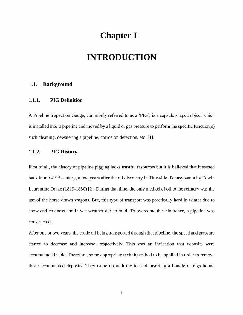
In order to move the PIG forward, the fluid is pumped upstream of the PIG by providing a required
amount of pressure depending on the location of the PIG at that instant i.e. this pressure is a
function of time.
Figure III-3 shows the PIG during pigging process along with its Free Body Diagram (FBD).
Figure III-3: Free Body Diagram
Page 27
18
By applying the Newton’s second law of motion [19, p.138] with a balance of forces acting on the
PIG along the normal and tangential directions, the dynamic equations are derived.
Firstly, along the normal direction,
cosc nN F mg ma (3.6)
where
N - Reaction force
m - Mass of the PIG
θ - Angular displacement of the PIG
We know that the normal acceleration,
2
n
Va
R (3.7)
where R – Pipeline centerline radius
And the velocity is
ds
Vdt
(3.8)
Recall that the distance along the PIG’s path is given by
ds Rd (3.9)
Therefore,
dV R
dt
V R
(3.10)
Page 28
19
And then, the normal acceleration is given as
2na R (3.11)
By substituting Eq. (3.5) and (3.11) into Eq.(3.6), we get
2coscN ldp mg mR
2coscN ldp mg mR (3.12)
And secondly, along the tangential direction,
sinf tF F mg ma (3.13)
with fF being the friction force
We know that the force due to fluid pressure is
2
4F d p
(3.14)
And by using the Coulomb’s law of friction [20, p. 338], the friction force is calculated as
fF N (3.15)
Replacing Eq. (3.12) into Eq.(3.15), we get
2cosf cF ldp mg mR (3.16)
Recall that the tangential acceleration is
t
dVa
dt (3.17)
Page 29
20
Hence,
2
2
t
d da R
dt dt
dR
dt
ta R (3.18)
Substituting Eq.(3.14), (3.16) and (3.18) into (3.13), we get
2 2cos sin4
cd p ldp mg mR mg mR
After arrangement, we get
2
24 sin coscd p ldp g
mR mR R
(3.19)
This equation is a nonlinear second-order differential equation with respect to parameter θ and
should be solved numerically. Normally, using MatLab Software, an algorithm of Runge-Kutta 4th
order method can be developed along with initial conditions to determine the parameter θ in terms
of time t. Consequently, the position and velocity of the PIG can be determined [21, pp. 569-578].
However, the main challenge is to determine the amount of pressure required to push the PIG and
keep the velocity within the required range. Mainly, this pressure would depend on the properties
of the polyurethane foam because during the PIG motion, there are some fluctuations which
generate more unpredictable friction. This uncertainty in the pressure to be provided makes the
analytical modelling unsuitable for this type of analysis.
Page 30
21
Since the above equation is a second-order nonlinear differential equation and the PIG is made in
polyurethane, we can deduce that the analysis of a PIG motion in a pipeline is a highly nonlinear
transient dynamic analysis.
3.2. Numerical Simulation
For solving most engineering problems, a numerical simulation software is the best tool to rely on.
An efficient and effective Computer Aided Engineering (CAE) tool for static, transient and
dynamic analysis can be considerably applied in engineering for model design, optimization and
simulation [22].
However, among the available commercial finite element software, ANSYS LS-DYNA has been
widely utilized and proved to be more advantageous in calculating and simulating nonlinear
dynamics problems.
ANSYS LS-DYNA integrates the Livermore Software Technology Corporation (LSTC)’s LS-
DYNA, an explicit finite element program with the pre-/post-processing power of the ANSYS
software. The explicit time integration scheme applied by LS-DYNA gives out fast and accurate
results for short-time, quasi-static or dynamics problems with large deformations and multiple
nonlinearities and complex contact or impact problems. Such problems are mostly found in metal
forming, drop testing, crashworthiness, pendulum impact test, etc.
Therefore, this powerful pairing helps engineers to model the structure in ANSYS Workbench,
solve the explicit dynamics in LS-DYNA and process the results using the standard ANSYS post-
processing tools [17, p. 1].
Page 31
22
3.2.1. Explicit Time Integration Scheme
The explicit time integration scheme used by LS-DYNA is based on the central difference method.
From the D’Alembert’s principle, the general equation of equilibrium for a damped system is [23,
pp. 499-500]
int extI DF F F F (3.20)
where int, , and I D extF F F F are the inertia force, damping force, internal force and externally applied
force, respectively.
I
D
F M u
F C u
(3.21)
When the system has a linear behavior, the internal force is
intF K u (3.22)
where , and M C K are the diagonal mass, damping and stiffness matrices of the system;
, and u u u are the displacement, velocity and acceleration vectors, respectively.
Therefore, the equation of motion becomes a linear ordinary differential equation
extM u C u K u F (3.23)
However, if the system is of a nonlinear behavior, the internal force becomes a nonlinear function
of displacement i.e. intF u which leads to a nonlinear ordinary differential equation of form
int extM u C u F u F (3.24)
Page 32
23
And this is where the complexity arises and ANSYS LS-DYNA has to come into play to solve this
sort of equation.
During integration, these matrices remain unaltered as they are time-independent. For such a
situation, an explicit scheme is recommended as the response quantities are determined in terms
of the previously obtained results of acceleration, velocity and displacement.
Throughout this method, the integration domain is discretized into a finite number of equally
spaced points, known as mesh or grid points and the solution is obtained at these individual points.
By considering a displacement-time curve shown in the Figure III-4, the run-time is divided into
equal segments with an interval of t and the initial displacement and velocity are supposed to be
known.
0
0
0
0
u t u
u t u
(3.25)
By using the central difference method, the velocity and acceleration at grid point i are calculated
as
1 1
12i i i
u u ut
(3.26)
1/2 1/2
1i i i
u u ut
(3.27)
Page 33
24
Figure III-4: Central Difference Method
To find the acceleration value at point node i, the velocities at the middle of the time interval t
around i have to be determined.
1/2 1
1/2 1
1
1
i i i
i i i
u u ut
u u ut
(3.28)
By replacing Eq. (3.28) into Eq.(3.27), we get
1 1
1 1 1i i i i iu u u u u
t t t
(3.29)
1 12
1i i i i iu u u u u
t
1 12
12i i i iu u u u
t
(3.30)
Page 34
25
Now, these difference formulas (Eq. (3.26) &(3.30)) can be expressed in terms of displacement
vector as
1 1
1
2n n nu u u
t
(3.31)
1 12
12n n n nu u u u
t
(3.32)
And the equation of motion at time becomes
intn nn n extM u C u F u F (3.33)
Substituting andn nu u from Eq. (3.31) & (3.32) respectively into Eq.(3.33), we get
1 1 1 1 int2
1 12
2 n nn n n n n extu u u M u u C F u Ftt
(3.34)
1 1 int2 2 2
1 1 2 1 1
2 2 n nn n n extM C u M u M C u F u Ft tt t t
1 int 12 2 2
1 1 2 1 1
2 2n nn ext n nM C u F F u M u M C ut tt t t
Now, let us,
2
1 1M + C = M
2ΔtΔt (3.35)
and
n
Page 35
26
1n n nn n
int 2ext ext2
2M
Δt
1 1F - F u + {u } - M - C {u } = F
2ΔtΔt (3.36)
then
1 nn
extM {u } = F (3.37)
where M is the effective mass matrix and nextF is the effective force vector.
By solving Eq.(3.37), the displacement at time n+1, 1nu is obtained. And the velocity and
acceleration at time n are calculated by replacing these values of 1nu .
When the time step is small, the stiffness term intF u will not vary significantly over the step.
For the time integration of nonlinear dynamics systems, there is no convenient verification to
calculate the time step. However, for stability reasons, LS-DYNA has provided a default scale
factor of 0.9 to decrease the time step [23, p. 489].
0.9 criticalt t (3.38)
where the critical time step size, criticalt is computed based on Courant-Friedrichs-Levy criterion
critical
lt
c (3.39)
with l being the characteristic length of the element and c the wave speed which is
E
c
(3.40)
where E - Young’s Modulus and - density.
Page 36
27
3.2.2. ANSYS LS-DYNA Workbench
According to Finite Element Method (FEM), there are several steps that must be covered to
perform a numerical simulation, however for an explicit solver like LS-DYNA, these steps are a
bit different. In order to be successful, these are the steps to be covered:
Material properties definition
Geometrical modelling
Finite element meshing
Contact definition
Pre-processing
(a) Material properties definition
Generally, in ANSYS Workbench, the material properties are entered in the Engineering Data
section. In this study, the pipeline is made of stainless steel while the PIG is made of medium
density polyurethane foam of 70 shore A durometer.
To get its Young’s Modulus, Eq. (1.1) was applied.
Table III.1. Material properties
Stainless Steel Polyurethane foam
Density, ρ 7750 kg/m3 100 kg/m3
Young’s Modulus, E 1.93E5 MPa 10.106 MPa
Poisson’s Ratio, ν 0.31 0.33
Page 37
28
(b) Geometrical modelling
Basically, the geometry was easily designed in SolidWorks [24] and then imported into ANSYS
Workbench. The PIG is of bullet nose shape for negotiating the bend line. The pipeline is
composed of two horizontal pipes and an elbow, as illustrated in Figure III-5. As the PIG diameter
is larger than that of the pipeline, a PIG launcher, which is an oversized pipe, together with a
reducer were added to the inlet of the pipeline and a PIG receiver, which is also an oversized pipe,
along with another reducer were added to the exit of the pipeline to hold the PIG in place before
and after the pigging process.
Figure III-5: PIG-Pipeline model in SolidWorks
Diametrically, the pipeline was split into four (4) sections around its central axis. This was done
to help the mesh generation process.
Page 38
29
Figure III-6: PIG-Pipeline model in ANSYS Design Modeler
In ANSYS Design Modeler, those parts of pipeline are assembled together to form a multibody
part so that their respective nodes are connected in a smooth way to get a good mesh.
(c) Finite element meshing
Fundamentally, the discretization of a model plays a major important role during Finite Element
Analysis (FEA) since the accuracy of the time integration results highly depends on the mesh
quality. Hence, the increase in number of grids improves the accuracy, but also the calculation
time increases. So, it’s up to the designer to make a bold decision based on the accuracy needed
and the computer performance.
As mentioned earlier, in order to get fast and accurate results, LS-DYNA uses an explicit time
integration scheme (see page 22). Therefore, the physics preference was set to explicit.
Page 39
30
Again, considering that the PIG is made of medium density polyurethane and the pipeline in
stainless steel, the pipeline stiffness behavior was set to rigid. This helps to greatly reduce the CPU
calculation time needed to perform an explicit analysis. This is due to the fact that mainly, most of
the contact surroundings are meshed and a single mass element is generated at the model centroid
[25, p. 327].
(i) Pipeline meshing
During the meshing setup, edge size and sweep method controls were applied to the pipeline to
generate pure hex meshes or elements. A pure hex mesh provides only one integration per element,
hence this technique is beneficial as it reduces the computational time [26].
Figure III-7: Meshed pipeline
Page 40
31
(ii) PIG meshing
For the PIG discretization, a body size control was applied as the smallest element size is the one
which controls the time step to be used during the calculation. Afterwards, a multizone method
control was applied. This method works on the same principle as the sweep method control.
Furthermore, it automatically slices the geometry into more sweepable bodies.
Finally, to adequately capture the region involved in frictional contact, inflation control was set to
get a finer mesh for the layers of the PIG’s surface.
Figure III-8: Meshed PIG
Page 41
32
Figure III-9: Meshed PIG-Pipeline model, sectional view
(iii) Mesh Quality
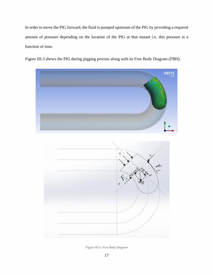
A generation of 40335 nodes and 31472 elements was obtained during this discretization process.
For checking the mesh quality, the skewness is used. A Skewness is an indicator to show much a
face or cell is close to being equilateral or equiangular.
A skewness of zero (0) is the best possible and a skewness of one (1) is never favored according
to ANSYS User’s Guide [25, pp. 136-138].
Page 42
33
Figure III-10: Ideal and Skewed Elements
As it can be seen in the figure below, the average skewness is 9.8624e-2, which is close to 0 value.
Therefore, the generated mesh is of good quality.
Page 43
34
Figure III-11: Skewness
(d) Contact definition
As said earlier, when the PIG is set in motion, it fluctuates as it moves and consequently, more
frictional contact is induced. Furthermore, this contact is a three-dimensional contact type.
Analytically, this type of friction can’t be calculated. Therefore, this is one of the reasons to utilize
ANSYS LS-DYNA to analyze this behavior and afterwards draw a conclusion based on the
obtained results.
First of all, when two bodies are sliding on each other, interface is formed. One of the sides is
called the slave side while the other is called the master side. Nodes located on those sides are
designated as slave and master nodes, respectively.
In order to handle contact problems, LS-DYNA has implemented three methods:
Page 44
35
Kinematic constraint method
Penalty method
Distributed parameter method
This study will only be limited to the penalty method. More details about all these methods can be
found in LS-DYNA Theory Manual [23, pp. 523-525].
A penalty method consists of placing normal interface springs between all penetrating nodes and
the contact surface. This obeys the Coulomb formulation whereby the frictional algorithm utilizes
the equivalence of an elastic plastic spring.
By applying this method, the penetration of the slave node through the master surface is checked.
If it is so, two forces are applied between the slave node and its contact point [27].
Interface force
Frictional force
(i) Interface force
The interface force also called restoring force, nF is the force which restrains the two parts to
penetrate each other. This force is normal to the master surface and its magnitude is proportional
to the amount of penetration as shown in Figure III-12.
nF kx (3.41)
where,
x - penetration of the slave node
k - stiffness factor for the master segment and is expressed as
Page 45
36
2KA
kV
(3.42)
Where,
- penalty scale factor
K - material bulk modulus
A - penetrated segment area
V - penetrated segment volume
Figure III-12: Contact basics
(ii) Frictional force
The frictional force, also called interface shear force, fF is the shear force that is parallel to the
penetrated master segment and its magnitude is proportional to the interface force.
Page 46
37
f nF F (3.43)
where is the instantaneous coefficient of friction
When the contacting surfaces are at rest, the coefficient of friction is called static coefficient of
friction, s and when those surfaces are in relative motion, the coefficient of friction is called
dynamic or kinetic coefficient of friction, d . Usually, the latter is smaller.
Oden and Martins [28] provided a model on how the friction coefficient decays exponentially from
the static value to the dynamic value based on this function
cvsd d
e
(3.44)
where
c is the decay constant
v is the relative velocity or slip rate and is expressed as
e
vt
(3.45)
where
e is the incremental move of the slave node
t is the time step size
Page 47
38
Figure III-13: Exponential decay frictional model
After going through on how LS-DYNA defines and treats contacts, especially friction, the friction
details were input into ANSYS LS-Dyna Workbench.
Figure III-14: Frictional contact details
Page 48
39
The static coefficient of friction, s , dynamic coefficient of friction,
d and decay constant, c
were set to 0.4, 0.25 and 1, respectively. An asymmetric behavior was selected since the two bodies
are of different materials.
(e) Pre-processing
Generally, the bodies involved in an explicit dynamic system are at rest, unconstrained and stress
free [29]. Therefore, initial conditions, loads and/or constraints are required for solving.
In ANSYS LS-DYNA Workbench, this step is called general pre-processing and sometimes it is
referred to as a mechanical setup where also analysis settings are added to this section.
(i) Loads
For a better analysis, PIGs of different diameters were considered and the driving pressure was
applied as a variable depending on the instantaneous position of the PIG to keep the PIG moving
in the pre-required velocity range.
From the figure below, it can be noted that the pressure is constant in the straight pipe and variable
in the elbow by decreasing as it enters the elbow and increasing as it exits the elbow.
Page 49
40
Figure III-15: Variable pressure
(ii) Constraints
Among the available constraints in ANSYS LS-DYNA, the applied constraints are:
Rigid body constraint
Contact properties
(1) Rigid body constraint
As the pipeline is rigid and not expected to move, a rigid body constraint was applied and
constrained the pipeline to be fixed in all directions during the whole pigging process.
Page 50
41
Figure III-16: Rigid body constraint
(2) Contact properties
This section helps to improve the contact behavior, especially the friction. This is where the contact,
type, formulation, soft constraint formulation, etc. are defined. In this study, as we already know,
the PIG is of foam. Hence, a soft constraint formulation was set to soft constraint. This is a key
property as it prohibits the PIG to traverse the pipeline once it enters the elbow section. The
remaining contact properties were kept as default.
Page 51
42
Figure III-17: Contact properties
Here, is what happened if the soft constraint is not applied.
Figure III-18: Soft constraint not applied
In this case, the PIG traverse the pipeline as a curved section is not part of the pipeline.
Page 52
43
(iii) Analysis settings
Generally, in order to get trustworthy results, analysis settings must be set with precaution and
care. In ANSYS LS-DYNA, analysis settings are divided into nine (9) groups. But, the most
important and relevant analysis settings about this study will be discussed in detail.
(1) Step controls
The step controls are used for controlling the time step size and end time for which the simulation
is expected to run.
The time step safety factor was kept as default i.e. 0.9 as it is recommended to help the calculation
stability. This is done in respect of Eq. (3.38).
In addition to this, automatic mass scaling has been used. Mass scaling consists of increasing the
time step size by scaling up the density of small elements as long as they use to control the time
step. This technique is for reducing the run-time and best used in analysis where the velocity is
low and the kinetic energy is very small compared to the internal energy.
(2) Solver controls
The solver controls are used to control the precision and unit system for the solver. When a
dynamics problem under study is of low velocity or contacts are present, double precision is
advised even though it does consume a large memory for calculation. According to this
recommendation, solver type was set to double precision.
(3) Hourglass controls
Hourglassing is a phenomenon by which individual elements are highly distorted whilst the overall
mesh section remains intact. Thus, hourglass modes are non-physical, zero-energy modes of
Page 53
44
deformation that produce zero strain and no stress [30]. These distorted elements have much
shorter periods and hence, they affect the simulation results. Therefore, they should be inhibited.
In this study, since the PIG is made of foam and its velocity is low, exact volume Flanagan-
Belytschko stiffness form was selected as hourglass type [23].
Page 54
45
Chapter IV
RESULTS AND DISCUSSION
Once the solution is obtained, the next challenge is to check and validate the processed results.
This step is called post-processing.
For an explicit dynamics analysis, results are obtained from:
Structural probes: which are used to display results such as deformation, strain, stress,
position, velocity, acceleration, etc.
Worksheet tab: which is mostly used to get and display “user defined results”.
4.1. Velocity
Figure IV-1: Velocity
Page 55
46
Recall that in order to get a nearly constant speed of about 5m/s, a variable pressure was applied
(see Page 39). Note how the velocity is decreasing and increasing as the PIG enters and exits the
elbow, respectively
4.2. Stress and Strain
Here, are the screenshots of the PIG’s stress at different locations in the pipeline.
Figure IV-2: PIG's stress at different locations in the pipeline
From the above screenshots, it can be seen that the PIG is more deformed in the elbow than in the
straight sections of the pipeline.
Page 56
47
Figure IV-3: Stress
Figure IV-4: Strain
As it had been mentioned earlier, by increasing the PIG’s diameter, an interference occurs. This
phenomenon can be easily recognized in the pipeline straight section (see Figure IV-3 and Figure
Page 57
48
IV-4). However, once the PIG is in the curved section, the large deformation has more impact,
leading to the interference effect being not appreciable.
4.3. Non-dimensional analysis
As this study was carried out by varying the PIG diameter, a non-dimensional analysis can be
performed to get an overall view about pigging process.
The parametrized time,
c
d
v (4.1)
The time coefficient,
t
t
(4.2)
The pressure coefficient,
0*c
p pp
p
(4.3)
where d - PIG diameter
cv - characteristic velocity
t - calculation time
p - instantaneous pressure
0p - instantaneous pressure for PIG without interference
cp - static interference contact pressure (see Eq. (3.1)).
Page 58
49
Figure IV-5: Pressure coefficient vs Time Coefficient
Considering the figure above, it can be observed that *p is constant throughout the whole process
regardless of the PIG size to be inserted. In this study, *p was found to be equal to 0.8.
However, some exceptions are noted in different locations of the pipeline. These are at the very
start and end of the process and also at the entrance and exit of the elbow due to entering a different
section of the pipeline.
Page 59
50
Chapter V
CONCLUSION AND RECOMMENDATIONS
5.1. Conclusion
The main goal of the dynamics analysis and numerical simulation of PIG motion in a pipeline is
to find the optimal pressure required to move the PIG by keeping the speed in the required range.
This project implements the simulation of the pigging process using ANSYS LS-DYNA and study
the effect of various parameters. It was conducted on a medium density polyurethane foam PIG.
The model was easily designed in SolidWorks and then imported into ANSYS for finite element
modeling. The finite element meshing was performed carefully for better results especially by
applying the sweep method and multizone method controls for an effective integration and the
inflation control to capture the layers involved in the friction region.
Parametrically, changing the PIG dimensions, the applied pressure is observed how it varies all
the way of the pipeline by keeping the velocity in the recommended range. Additionally, the results
obtained from ANSYS were exported to MatLab for further analysis and good understanding of
the PIG behavior throughout the process.
After conducting this research, the following conclusions were drawn:
Mathematical or analytical modeling can’t do the dynamics analysis alone as too many
irregular parameters are involved during the pigging process. Numerical simulation should
be performed as it takes into accounts all those parameters and fairly estimates what truly
happens on the field.
Page 60
51
For a good pigging process, an interference should occur as a result of PIG diameter being
larger than the pipeline inner diameter.
Also, as we have seen, the pressure should not be constant. It is constant in the straight pipe
and variable in the curved section in order to have a nearly constant speed.
And finally, the ratio (i.e. *p ) of the difference between instantaneous pressure and
reference pressure over the static interference contact pressure is constant.
In this thesis, the simulated pigging process has proved successful, however there is still room for
more improvement. In the next section, some recommendations are listed in that regard.
5.2. Recommendations
With the dynamics finite element simulation, much valuable information has been obtained, such
as about how the PIG moves, how the PIG gets deformed (stress and strain), etc. Those are
observed by viewing the output, plotting graphs and producing results animations. Therefore,
before introducing the PIG in the pipeline on the site, it is a better practice to perform the
simulation and observe how the PIG will behave during the process since on the field, many
accidents have been occurring due to not closely predicting its behavior beforehand.
Throughout this study, a medium density polyurethane foam PIG has been utilized. In our future
work, we are planning to shift our focus on a hard density polyurethane foam PIG because if care
is not taken, the pipeline may burst especially once the PIG arrives in the curved section.
Furthermore, the fluid flow analysis will have to be performed since it may have an impact on the
pigging process. This is mostly notable in the elbow due to the head loss.
Page 61
52
References
[1] PIGging Products & Services Association, An Introduction to Pipeline PIGging: Gulf
Professional Publishing, 1995.
[2] C. J. Cleveland and B. Black. (2008, April 01). Drake, Edwin Laurentine. Available:
http://www.eoearth.org/view/article/151795/
[3] R. Davidson, An Introduction to Pipeline PIGging: Halliburton Pipeline and Process
Services-PIGging Products and Services Association, 2002.
[4] J. N. H. Tiratsoo, Pipeline PIGging Technology, 2 ed. Houston, TX: Gulf Professional
Publishing, 1992.
[5] H. J. Qi, K. Joyce, and M. C. Boyce, "Durometer Hardness and the Stress-Strain Behavior
of Elastomeric Materials," Rubber Chemistry and Technology, pp. 419-435, 2003.
[6] R. Taylor, "A Guide to Shore Durometers," vol. 2016, ed, 2014.
[7] Central Intelligence Agency, "Pipelines," Central Intelligence Agency2014.
[8] A. E. McDonald and O. Baker, "Multiphase Flow in Pipelines," Oil & Gas Journal, pp.
68-71 (June 15); 171-175 (June 122); 118-119 (July 176), 1964.
[9] J. M. Sullivan, "An Analysis of The Motion of PIGs Through Natural Gas Pipelines,"
Master of Science, Mechanical Engineering, Rice University, Houston, Texas, 1981.
[10] A. O. Nieckele, A. M. Braga, and L. F. Azevado, "Transient PIG Motion Through Gas and
Liquid Pipelines," Journal of Energy Resources Technology, vol. 123, pp. 260-269, 2001.
[11] T. T. Nguyen and S. B. Kim, "Modeling and Simulation for PIG Flow Control in Natural
Gas Pipeline," KSME International Journal, vol. 15, pp. 1165-1173, 2001.
[12] T. T. Nguyen, D. K. Kim, Y. W. Rho, and S. B. Kim, "Dynamic Modeling and Its Analysis
for PIG Flow through Curved Section in Natural Gas Pipeline," in 2001 IEEE International
Page 62
53
Symposium on Computational Intelligence in Robotics and Automation, Banff, Alberta,
Canada, 2001, pp. 492 - 497.
[13] D. K. Kim, S. H. Cho, S. S. Park, Y. W. Rho, and H. R. Yoo, "Verification of the Theoritical
Model for Analyzing Dynamic Behavior of the PIG from Actual PIGging," KSME
International Journal, vol. 9, pp. 1349-1357, 2003.
[14] M. Saeidbakhsh, M. Rafeeyan, and Ziaei-Rad, "Dynamic Analysis of Small PIGs in Space
Pipelines," Oil & Gas Science and Technology, vol. 64, pp. 155-164, 2009.
[15] W. Wang, S. Song, S. Zhang, and D. Yu, "Impact analysis of PIGging in shield segment
of gas pipe," in 2012 IEEE International Conference on Mechatronics and Automation
(ICMA), Chengdu, China, 2012, pp. 203-207.
[16] M. Mirshamsi and M. Rafeeyan, "Dynamic analysis and simulation of long PIG in gas
pipeline," Journal of Natural Gas Science and Engineering, vol. 23, pp. 294-303, 2015.
[17] ANSYS, Inc,, ANSYS LS-DYNA User's Guide Release 12.1. Canonsburg, PA 15317, U.S.A:
ANSYS, Inc, 2009.
[18] R. G. Budynas and J. K. Nisbett, Shigley's Mechanical Design Engineering, 10 ed. New
York: McGraw-Hill Education, 2014.
[19] J. L. Meriam and L. G. Kraige, Engineering Mechanics: Dynamics, 7 ed. vol. 2: Wiley,
2012.
[20] J. L. Meriam and L. G. Kraige, Engineering Mechanics: Statics, 7 ed. vol. 1: Wiley, 2011.
[21] C. Chapra, Applied Numerical Methods with MATLAB for Engineers and Scientists, 3 ed.
New York: McGraw-Hill Education, 2011.
[22] Y. Liu, "ANSYS and LS-DYNA used for structural analysis," International Journal of
Computer Aided Engineering and Technology, vol. 1, 2008.
Page 63
54
[23] J. O. Hallquist, LS-DYNA Theory Manual. Livermore, California: Livermore Software
Technology Corporation, 2006.
[24] Dassault, Systems. (January 13). SolidWorks. Available: http://www.solidworks.com/
[25] ANSYS, Inc,, ANSYS Meshing User's Guide Release 16.0. Canonsburg, PA 15317, U.S.A:
ANSYS, Inc., 2015.
[26] ANSYS, Inc,. (2012, October 30, Introduction to ANSYS LS-DYNA Release 14.5, Lecture
7, Explicit Meshing.
[27] J. D. Reid and N. R. Hiser, "Friction Modeling Between Solid Elements," International
Journal of Crashworthiness, vol. 9, pp. 65-72, 2004.
[28] J. T. Oden and J. A. C. Martins, "Models and computational methods for dynamic friction
phenomena," Computer Methods in Applied Mechanics and Engineering, vol. 52, pp. 527-
634, 1985.
[29] ANSYS, Inc,. (2015, February 12, Workbench LS-DYNA (ACT Extension) Training,
Release, Lecture 3, Workbench LS-DYNA Basics.
[30] LS-DYNA Support. (February 28). Hourglass. Available:
http://www.dynasupport.com/howtos/element/hourglass
Page 64
55
파이프라인에서 피그 거동 동적 해석 연구
파브리스
전남대학교대학원 기게설계 공학과
(지도교수: 김기성)
(국문초록)
파이프라인은 석유 생산물이나 천연가스 등을 이송하기 위한 긴 파이프이다. 건설 후
얼마간 시간이 지나면 파편이나 잔류물이 내부에 끼게 되고 파이프라인을 통한 이송이
비효율적으로 된다. 이송성능을 다시 회복하기 위해서는 적절한 방법으로 파이프라인을
클리닝하고 물리적 상태를 검사할 필요가 있다. 가장 많이 이용하는 방법은 파이프라인
검사 도구(PIG)를 유체로 밀어 진행시키는 것이다.
본 연구의 대상인 PIG 는 중밀도 폴리우레탄 폼으로 제작된 것으로 파이프라인 내경보다
약간 큰 외경을 갖도록 만들어져 있다. 파이프라인은 직선파이프와 엘보우로 되어 있으며
구동력은 유체 압력이다.
PIG 의 동력학적인 거동과 변형을 파악하기 위하여 PIG 에 작용하는 모든 힘을 고려하여
수학적 모델링을 수행하였는데 뉴턴의 운동 제 2 법칙을 적용하면 비선형 2 차
Page 65
56
미분방정식이 얻어진다. 더구나 PIG 의 재질이 우레탄 폼으로 되어 있기 때문에 이와
같은 해석 방법은 고도로 비선형이고 시간적으로 변화하는 동적해석을 수반한다.
이러한 비선형 동적 문제를 해석할 수 있는 상용 코드로 ANSYS LS-DYNA(비선형 동적
유한요소법 코드)가 적합하며 따라서, 이를 이용하여 PIG 거동을 해석하였다.
PIG 와 파이프 간의 직경간섭 효과를 조사하였는데 PIG 가 같은 속도로 진행하기 위해
필요한 압력을 계산하였다. 파이프의 직선구간과 곡선구간에서 필요한 압력을
일반화하기 위해 이 압력을 적합한 기준값으로 표준화하였는데 직경간섭값에 따라
비슷한 경향을 나타내었다.
이 논문에서 적용한 접근방법이 중간 밀도의 폴리우레탄 폼 PIG 의 동력학적인 거동과
응력해석 에 잘 적용될 수 있음을 확인하였다.
Page 66
57
Dedicated
To
My beloved
Parent
Page 67
58
Acknowledgement
This research was carried out under the supervision of Professor Kim Ki-Seong from the
Department of Mechanical Design Engineering at Chonnam National University and was
conducted in partnership with Koins Co., Ltd.
I would like to take this opportunity to extend my sincere gratitude and immeasurable appreciation
to many great people who have contributed in one way or another to make this Masters possible.
First and foremost, I wish to express my utmost gratitude to The Almighty God without His
blessing and inspiration, nothing is possible.
I would like to give my deepest gratitude towards Professor Kim Ki-Seong for giving me this
invaluable opportunity to work on this research. His patient guidance, enthusiastic encouragement,
constructive suggestions and support throughout my study. He did not only help me to accomplish
this thesis, but also inspired me to have a rigorous attitude about researching, being hardworking
and a love for engineering. Getting the chance to work in his laboratory, it was a blast. I am really
thankful to him.
My heartfelt thanks to my fellow labmates for sharing with me their knowledge and ideas, teaching
me the lab culture and making an exciting and fun environment to learn.
I would like to express my eternal appreciation towards the people who mean a world to me, my
parents and family. I can’t imagine a life without their warm love, blessings, unceasing patience
and endless support.
Last but not least, my thanks goes to all my friends who encouraged me along the way. Especially,
a debt of gratitude is owed to TWIZIHIRWE KAYIHURA Marie Paule for her never ending
motivations during my entire studies despite being far away of me.