Dynamic Analysis of Planar Solid Oxide Fuel Cell Models...

1

omard

ahtSilb�scls

thladbpTft

p

J

Downloa

Handa Xi

Jing Sun1

Department of Naval Architecture and MarineEngineering,

University of Michigan,Ann Arbor, MI 48109

Dynamic Analysis of Planar SolidOxide Fuel Cell Models WithDifferent Assumptions ofTemperature LayersAs solid oxide fuel cell (SOFC) technology is rapidly evolving, high-fidelity mathematicalmodels based on physical principles have become essential tools for SOFC system designand analysis. While several SOFC models have been developed by different groups usingdifferent modeling assumptions, little analysis of the effects of these assumptions onmodel performance can be found in literature. Meanwhile, to support system optimizationand control design activities, a trade-off often has to be made between high fidelity andlow complexity. This trade-off can be influenced by the number of temperature layersassumed in the energy balance to represent the SOFC structure. In this paper, we inves-tigate the impact of the temperature layer assumption on the performance of the dynamicplanar SOFC model. Four models of co-flow planar SOFCs are derived using the finitevolume discretization approach along with different assumptions in the number of tem-perature layers. The model with four temperature layers is used as the baseline model,and the other models aimed at reducing the complexity of the baseline model are devel-oped and compared through simulations as well as linear analysis. We show that themodel with as few as two temperature layers—the solid structure and air bulk flow—isable to capture the dynamics of SOFCs, while assuming only one temperature layerresults in significantly large modeling error. �DOI: 10.1115/1.2971055�

IntroductionGiven their high efficiency, low emissions, and flexible fueling

ptions, solid oxide fuel cells �SOFCs� have great potential inany applications including stationary power plants and mobile

uxiliary power unit systems �1�. Among different SOFC configu-ations, planar SOFCs have received increasing attention recentlyue to their compact size and higher power density and efficiency.

As SOFC technology evolves, mathematical models that canccurately describe steady-state and dynamic behaviors of SOFCsave become critical tools for SOFC system design and evalua-ion. Several dynamic models have been reported for planarOFCs in the literature �2–9� and used to investigate their dynam-

cs. Transient operating issues such as slow load following andarge overshoots of temperature and temperature gradient haveeen identified in the dynamic response of SOFC systems8,10–12�, necessitating feedback control strategies to improve theystem transient performance. In order to facilitate model-basedontrol design and analysis, a simplified dynamic model with aow order that preserves the key dynamic characteristics of theystem is always desirable.

Among the planar SOFC dynamic models reported in the litera-ure, it has been recognized that different modeling assumptionsave been used by different groups, thereby leading to differentevels of model accuracy and complexity. For instance, differentssumptions of temperature layers to represent the temperatureistribution along the axis perpendicular to the cell plate haveeen used in these models, resulting in different numbers of tem-erature states in the energy balance dynamics of the fuel cell.able 1 summarizes the different temperature layer assumptionsound in the literature for dynamic planar SOFC modeling. Fiveemperature layers, i.e., fuel bulk flow, air bulk flow, positive

1Corresponding author.Manuscript received May 3, 2007; final manuscript received November 26, 2007;

ublished online November 6, 2008. Review conducted by Umberto Desideri.

ournal of Fuel Cell Science and TechnologyCopyright © 20

ded 08 Apr 2009 to 141.212.194.208. Redistribution subject to ASM

electrode–electrolyte–negative electrode �PEN� assembly, andfuel/air-side interconnectors, are assumed in the SOFC modelsdeveloped in Refs. �3,8�. In Refs. �5,6�, four temperature layersare used by considering the fuel and air-side interconnectors asone part for the cells in the middle of the SOFC stack. A three-temperature-layer assumption can be found in the models derivedin Refs. �2,4�, where the PEN and interconnector are combined asone temperature layer, called solid structure. In Refs. �7,9�, onlyone temperature layer is assumed.

By combining layers with similar steady-state and dynamiccharacteristics in temperature response, the energy balance dy-namics in the SOFC model can be simplified and the number oftemperature states in the model is minimized. This model reduc-tion, however, is only possible if the consequences of the simpli-fication can be fully understood and the trade-off between modelaccuracy and complexity thoroughly evaluated. However, limitedanalysis has been reported about the influence of the temperaturelayer assumption on the performance of the dynamic planar SOFCmodel. Campanari et al. compared steady-state planar SOFC mod-els with three �fuel, air, and solid structure� and nine �fuel, air,PEN, three in fuel-side interconnector, and three in air-side inter-connector� temperature layers in Ref. �13�, based on steady-statesimulation results. More recently, we studied the dynamic re-sponses of planar SOFC models with assumptions of one to fourtemperature layers �14�.

This paper extends the analysis presented in the conferencepaper �14�. A dynamic baseline model of the co-flow planar SOFCis first derived. Given the scope of this study, the description isfocused on the energy balance part. Finite volume discretizationapproach is applied to capture the spatial distribution of variablesinside the fuel cell. In this baseline model, four temperature lay-ers, i.e., fuel bulk flow, air bulk flow, PEN, and interconnector, areassumed, introducing four temperature states in the energy bal-ance dynamics for each discretization unit. Three different as-sumptions with reduced numbers of temperature layers are then
proposed for model simplification. The effects of these modeling
FEBRUARY 2009, Vol. 6 / 011011-109 by ASME

E license or copyright; see http://www.asme.org/terms/Terms_Use.cfm

amshhpi

latpa

Tf

R

�

�

�

�

0

Downloa

ssumptions on the performance of the dynamic planar SOFCodel are evaluated by comparing both steady-state and transient

imulations as well as performing linear analysis. As the endot-ermal direct internal reforming �DIR� activity in the SOFC couldave a strong influence on the dynamics of the fuel cell, the im-act of DIR on the selection of the temperature layer assumptions also investigated.

The rest of this paper is organized as follows: a dynamic base-ine model is first described for a co-flow planar SOFC. Differentssumptions of temperature layers for the SOFC modeling arehen proposed and compared to evaluate the impact of the tem-erature layer assumption on the model performance. Conclusionsnd future work are discussed at the end of this paper.

able 1 Different modeling assumptions of temperature layersound in literature

ef. Assumption of temperature layers

3,8� Five temperature layers:fuel bulk flowair bulk flow

PENfuel-side interconnectorair-side interconnector

5,6� Four temperature layersfuel bulk flowair bulk flow

PENinterconnector

2,4� Three temperature layers:fuel bulk flowair bulk flow

solid structure

7,9� One temperature layer:solid structure

Fig. 1 Co-flow planar SOFCs „dim

Fig. 2 Finite volume discretizati

11011-2 / Vol. 6, FEBRUARY 2009


2 Baseline Model of Co-flow Planar SOFCSFigure 1 illustrates the operating principle of the co-flow planar

SOFC considered in this paper. Six species, namely, CH4, CO,CO2, H2O, H2, and N2, are assumed in the fuel stream, and thefuel inlet composition depends on the type and operation condi-tion of the fuel reformer. Dry air is fed into the cathode of the fuelcell as oxidant and coolant. As shown in Fig. 1, besides the elec-trochemical reactions, the steam reforming �SR� and water gasshift �WGS� reactions in the fuel bulk flow are considered. Thus,all the reactions incorporated in the SOFC model are listed asfollows:

• SR: CH4+H2O→CO+3H2• WGS: CO+H2O↔CO2+H2• Oxidation �ox�: H2+O2−→H2O+2e−

• Reduction �red�: 0.5O2+2e−→O2−.

The planar SOFC is often considered as a distributed parametersystem in order to capture the spatial distribution along the flowfield for variables such as temperature, species concentration, andcurrent density �2–6,8,15�. The governing equations are describedusing either partial differential equations or discretization tech-nique. In this paper, the finite-volume discretization approach�8,13,16,17� is applied to derive the model for the co-flow planarSOFC shown in Fig. 1. Using this method, the cell is virtuallydivided into a user-defined number of small units along the bulkflow direction, as illustrated in Fig. 2, where the electrode andelectrolyte layers are considered as one assembly structure, calledthe PEN. These discretization units are integrated to form theSOFC model by imposing the gas flows, heat exchanges, andcurrent distribution relations.

Because of the high electrical conductivities of the interconnec-tors, the cell is assumed equipotential among the discretizationunits, and therefore we have

Uj = Ucell, j = 1,2, . . . ,J �1�

ions of the layers are not to scale…
ens
on for co-flow planar SOFCs

Transactions of the ASME


wtzcc

wdptdSpdct

Tfflc

wflctsos

J

Downloa

�j=1

J

ijAj = I �2�

here Uj and Ucell are the operating voltages of the jth unit andhe entire cell, respectively, J is the total number of the discreti-ation units, ij and Aj are the current density and the electrochemi-al reaction area, respectively, in the jth unit, and I is the totalurrent drawn from the cell. Uj can be calculated as follows:

Uj = UOCVj − � j, j = 1,2, . . . J �3�

here UOCVj is the open circuit voltage in the jth unit and can be

etermined by the Nernst equation �1,18�. � j represents the totalotential loss due to various sources, including the internal resis-ance, activation energy, and gas species diffusion. Equation �3�efines the polarization relation in the jth discretization unit in theOFC, where Uj is a function of local gas flow concentration,ressure, cell temperature, as well as current density. Detailedescription of the approach for calculating UOCV

j and � j in Eq. �3�an be found in Ref. �19�. and is omitted here to avoid duplica-ion.

For the jth discretization unit, the following are defined:

• nin,sf

j and nout,sf

j , sf � �CH4,CO2,CO,H2O,H2,N2�: the inletand outlet molar flux of species sf in the fuel bulk flow,respectively

• nin,sa

j and nout,sa

j , sa� �O2,N2�: the inlet and outlet molar fluxof species sa in the air bulk flow, respectively

• qin,fj and qout,f

j : the inlet and outlet enthalpy flux in the fuelbulk flow, respectively

• qin,aj and qout,a

j : the inlet and outlet enthalpy flux in the fuelbulk flow, respectively

From the mass and energy conservation in bulk flows, we have

nin,sf

j = nout,sf

j−1 �4�

nin,sa

j = nout,sa

j−1 �5�

qin,fj = qout,f

j−1 �6�

qin,aj = qout,a

j−1

j = 2, . . . ,J �7�

he boundary conditions, nin,sf

1 , nin,sa

1 , qin,f1 and qin,a

1 , depend on theuel and air inlets to the fuel cell. The outlet molar and enthalpyux in the fuel and air channels of each discretization unit can bealculated as follows:

nout,sf

j = uout,fj Csf

j �8�

nout,sa

j = uout,aj Csa

j �9�

qout,fj = uout,f

j �sf

Csf

j hsf�Tf

j� �10�

qout,aj = uout,a

j �sa

Csa

j hsa�Ta

j �

j = 1, . . . ,J �11�

here uout,fj and uout,a

j are the speeds of the fuel and air outletows in the jth unit, respectively. Csf

j and Csa

j are the speciesoncentrations in the fuel and air bulk flows, respectively. hs�T� ishe specific enthalpy of species s at temperature of T. Given themall pressure drop across the fuel cell, uout,f

j and uout,aj can be

btained using linear orifice relations and ideal gas law �8�. Thej j
pecies concentrations, Csf
and Csa, are determined by the mass

ournal of Fuel Cell Science and Technology


balance dynamics, and the fuel and air temperature, Tfj and Ta

j , bythe energy balance.

2.1 Mass Balance Dynamics. The mass balance dynamics ofgas species in the fuel and air bulk flows in the jth discretizationunit can be described as follows:

fuel: Csf= �nin,sf

− nout,sf�1

l+ �

k��SR,WGS,ox��sf,k

rk

1

df

sf � �CH4,CO2,CO,H2O,H2,N2� �12�

air: Csa= �nin,sa

− nout,sa�1

l+ �sa,redrred

1

da

sa � �O2,N2� �13�

where the superscript j of all the variables is omitted because theyall refer to the same discretization unit. This notation simplifica-tion will also be applied to other equations in the rest of this paper,due to the same reason. In Eqs. �12� and �13�, l is the length of thediscretization unit, �·,k is the stoichiometric coefficient in reactionk, rk is the kinetic rate of reaction k, and df and da are the heightsof the fuel and air channel, respectively. The reaction rates, rk, arecalculated following the approach used in Ref. �19�.

2.2 Energy Balance Dynamics. As mentioned in Sec. 1, oneor more temperature layers are usually assumed in SOFC model-ing to describe the temperature variation in the axis normal to thecell plate. Due to their small thickness and tight connection, thethree layers in the PEN structure are often assumed to have thesame temperature in dynamic SOFC models �2–9�. In the SOFCmodel developed in Ref. �8�, five temperature layers, i.e., PEN,fuel/air bulk flows, and fuel/air-side interconnectors are assumed.Note that, in the middle of a planar SOFC stack, the fuel/air-sideinterconnectors of adjoining cells are either manufactured as onepart or tightly packaged together. The fuel/air-side interconnectorsof adjacent cells can be treated as one temperature layer, called theinterconnector, to reflect this assembly structure in the middle ofthe stack. Since the model developed here is intended to describethe cell in the middle of a co-flow planar SOFC stack, we considerfour temperature layers, i.e., the fuel bulk flow, air bulk flow,PEN, and interconnector, in each discretization unit of the base-line SOFC model.

The temperatures in these four layers are calculated by solvingthe dynamic energy balance in each layer. The heat transfer con-sidered in the model includes the convection between the bulkflows and their surrounding solid structures, the conduction insolid layers as well as radiation between PEN and interconnectors.

The energy balance dynamics in the fuel flow can be expressedas follows:

d

dt��sf

Csfesf = �qin,f − qout,f�

1

l+ �kf ,PEN�TPEN − Tf� + kf ,I�TI

− Tf��1

df+ rox�hH2O�TPEN� − hH2

�Tf��1

df�14�

where esfis the specific internal energy of species sf. The first

term on the right hand side of Eq. �14� is due to the enthalpy fluxof the bulk flow, and the second term accounts for the convectiveheat exchange between the fuel flow and its surrounding solidlayers. The heat transfer coefficient can be obtained by assuming aconstant Nusselt number of 4 �20�. The last term of Eq. �14� iscaused by the enthalpy flux due to the ox reaction at the anode.

According to the relation for the ideal gas flow, esf=hsf

− psf/Csf

, where hsfis the specific enthalpy of species sf, we can

obtain

FEBRUARY 2009, Vol. 6 / 011011-3


tc

wlP

iircae

3T

es

S

JLWddl��

0

Downloa

Tf =1

�sfcv,sf

Csf

− �sf

�hsf�Tf� − RTf�Csf

+ �qin,f − qout,f�1

l

+ �kf ,PEN�TPEN − Tf� + kf ,I�TI − Tf��1

df+ rox�hH2O�TPEN�

− hH2�Tf��

1

df� �15�

Similarly, for the air flow, we have

Ta =1

�sacv,sa

Csa

− �sa

�hsa�Ta� − RTa�Csa

+ �qin,a − qout,a�1

l

+ �ka,PEN�TPEN − Ta� + ka,I�TI − Ta��1

da− 0.5rredhO2

�Ta�1

da�

�16�From the energy balance in the solid components in the SOFC,

he temperature dynamics in the PEN assembly and interconnectoran be described as follows:

TPEN =1

�PENcp,PENqcond,PEN

1

l− �kf ,PEN�TPEN − Tf� + ka,PEN�TPEN

− Ta��1

�PEN+ rox�hH2

�Tf� + 0.5hO2�Ta� − hH2O�TPEN��

1

�PEN

− iU1

�PEN+

2��TI4 − TPEN

4 �1/�I + 1/�PEN − 1

·1

�PEN� �17�

TI =1

�Icp,Iqcond,I

1

l− kf ,I�TI − Tf�

1

�I− ka,I�TI − Ta�

1

�I

−2��TI

4 − TPEN4 �

1/�I + 1/�PEN − 1·

1

�I� �18�

here qcond is the flux of heat conduction in the solid layers. Theast terms in Eq. �17� and �18� are due to the radiation between theEN and the interconnector.The dimension and material properties given in Ref. �5� for an

ntermediate-temperature anode-supported planar SOFC are usedn this paper for simulation and analysis. For the convenience ofeference, some geometry parameters are listed in Table 2. A dis-retization grid with 16 evenly distributed units is selected here asreasonable trade-off between model accuracy and simulation

fficiency �8�.

Analysis on Models With Different Assumptions ofemperature LayersAs shown in Table 1, different assumptions of temperature lay-

rs have been used in SOFC models developed by different re-

Table 2 Geometry parameters in SOFC model

ymbol Definition Unit Value

Total number of discretization units 16Cell length m 0.4Cell width m 0.1

a Air channel height m 0.001

f Fuel channel height m 0.001Length of discretization unit m L /J=0.025

I Thickness of interconnector m 0.001

PEN Thickness of PEN �m 570

earchers, leading to models with different complexities. In this

11011-4 / Vol. 6, FEBRUARY 2009


section, the impacts of different temperature layer assumptions onthe performance of the SOFC model are evaluated based on simu-lation results.

3.1 Model Assumptions With Reduced Number of Tem-perature Layers. In Sec. 2, four temperature layers, namely, fuelbulk flow �Tf

j�, air bulk flow �Taj �, PEN �TPEN

j �, and interconnector�TI

j�, are assumed in the energy balance dynamics, introducingfour temperature states to each discretization unit in the SOFCmodel. Given that our ultimate goal is to provide a dynamic modelwith low complexity for feedback control design and system op-timization, we attempt to minimize the number of temperaturelayers in the model assumption, thereby reducing the number oftemperature states, as long as the key dynamics of SOFC arepreserved in the simplified model.

With the four-temperature-layer baseline model described inSec. 2 also referred to as the 4T model�, three other models withreduced numbers of temperature states can be constructed, aslisted in Table 3.

• 3T: As the PEN assembly and the interconnector are thesolid components in the fuel cell, the model called 3T con-siders them as one temperature layer with the same tempera-ture profile and adopts the same assumption as used in Refs.�2,4�. In this model, three temperature layers, i.e., the fuelbulk flow, air bulk flow, and solid structure �consisting ofPEN and interconnector� are assumed.

• 2T: One state is for the temperature of the air bulk flow andthe other for the temperature of the remaining parts in eachdiscretization unit. This model assumption can be justifiedby Fig. 3, where the open-loop temperature response of thebaseline model at four different locations in the fuel cell,i.e., the temperature in the 1st �T1�, the 6th �T6�, the 11th�T11�, and the last �T16� discretization units, are shown. Dur-ing the simulation, the current load and gas inlet conditionsof the SOFC system switch at 100 s from part load to fullload setpoints that are listed in Table 4. These operatingparameters are obtained through system steady-state optimi-zation �12�. As can be seen from Fig. 3, the temperatures ofthe fuel bulk flow, PEN structure, and interconnector exhibitsimilar steady-state and dynamic responses, suggesting the

Table 3 Models with different assumptions of temperaturelayers

Model name Assumption of temperature layers

4T�baseline model�

Four layers: fuel �Tf�air �Ta�

PEN �TPEN�interconnector �TI�

3T Three layers: fuel �Tf�air �Ta�

solid structure �Tsol�TPEN=TI=Tsol

2T Two layers: air �Ta�solid structure �Tsol�Tf =TPEN=TI=Tsol

neglect energy of the gas accumulatedin the fuel channel

1T One layer: solid structure �Tsol�Tf =Ta=TPEN=TI=Tsol

neglect energy of the gas accumulatedin the fuel and air channels

possibility of combining these three parts as one tempera-



Ittb

to

Fi

Tr

C

AFOIAI

J

Downloa

ture layer. In addition, considering the small volume in thegas channels, the energy of the gas accumulated in the fuelchannel is neglected in the 2T assumption.

• 1T: Combining all four temperature layers into one gives the1T model, where all layers in one discretization unit areassumed to have equal temperature and the energy of the gasaccumulated in both fuel and air channels is neglected.

n order to isolate the effects of the reduced number of tempera-ure states, except for the energy balance dynamics, other parts inhe above three simplified models are kept the same as in theaseline 4T model.

While the governing equations of the temperature dynamics forhe baseline model have been derived in Sec. 2, equations forther models are listed as follows �note again that the superscript

j is omitted�:For 3T model: Tf, Ta, Tsol,

ig. 3 Open-loop temperature response at different locationsn the SOFC using the baseline 4T model

able 4 Operating parameters for the case with CPOXeformer

Full load Part load

urrent load, I �A� 320 160

ve. current density, i �A /cm2� 0.8 0.4

uel utilization ratio 90% 90%xygen/carbon ratio in CPOX 0.65 0.60

nlet temperature of reformate to SOFC �K� 991 963ir excess ratio 9.0 6.2

nlet temperature of air to SOFC �K� 991 963



Tf =1

�sfcv,sf

Csf

− �sf

�hsf�Tf� − RTf�Csf

+ �qin,f − qout,f�1

l

+ �kf ,PEN�Tsol − Tf� + kf ,I�Tsol − Tf��1

df+ rox�hH2O�Tsol�

− hH2�Tf��

1

df� �19�

Ta =1

�sacv,sa

Csa

− �sa



l

+ �ka,PEN�Tsol − Ta� + ka,I�Tsol − Ta��1

da− 0.5rredhO2

�Ta�1

da�

�20�

Tsol =1

�PENcp,PEN�PEN + �Icp,I�Iqcond,PEN

�PEN

l+ qcond,I

�I

l

− kf ,PEN�Tsol − Tf� − ka,PEN�Tsol − Ta� − kf ,I�Tsol − Tf�

− ka,I�Tsol − Ta� + rox�hH2�Tf� + 0.5hO2

�Ta� − hH2O�Tsol��

− iU� �21�

For 2T model: Ta, Tsol,

Ta =1

�sacv,sa

Csa

− �sa



l

+ �ka,PEN�Tsol − Ta� + ka,I�Tsol − Ta��1

da− 0.5rredhO2

�Ta�1

da�

�22�

Tsol =1


�PEN

l+ qcond,I

�I

l+ �qin,f

− qout,f�df

l− ka,PEN�Tsol − Ta� − ka,I�Tsol − Ta� + 0.5rredhO2

�Ta�

− iU� �23�

For 1T model: Tsol,

Tsol =1


�PEN

l+ qcond,I

�I

l+ �qin,f

− qout,f�df

l+ �qin,a − qout,a�

da

l− iU� �24�

3.2 Model Performance Comparison. The performance ofthese SOFC models, which assumed different temperature layers,are first compared using the simulation platform developed in Ref.

Fig. 4 Planar SOFC and CPOX system

�12�, where the SOFC system configuration illustrated in Fig. 4 is

FEBRUARY 2009, Vol. 6 / 011011-5


usstsSDe

pPt5dmtlbabO2

srsc

0

Downloa

sed. This system consists of a 25-cell co-flow planar SOFCtack, an external catalytic partial oxidation �CPOX� fuel proces-or and gas supply manifolds. Furthermore, in order to evaluatehe impacts of the strongly endothermal SR reaction on the modelimplification result, another case, where the fuel inlet to theOFC contains a relatively high fraction of CH4 and significantIR activity takes place in the fuel cell, is also discussed at the

nd of this section.

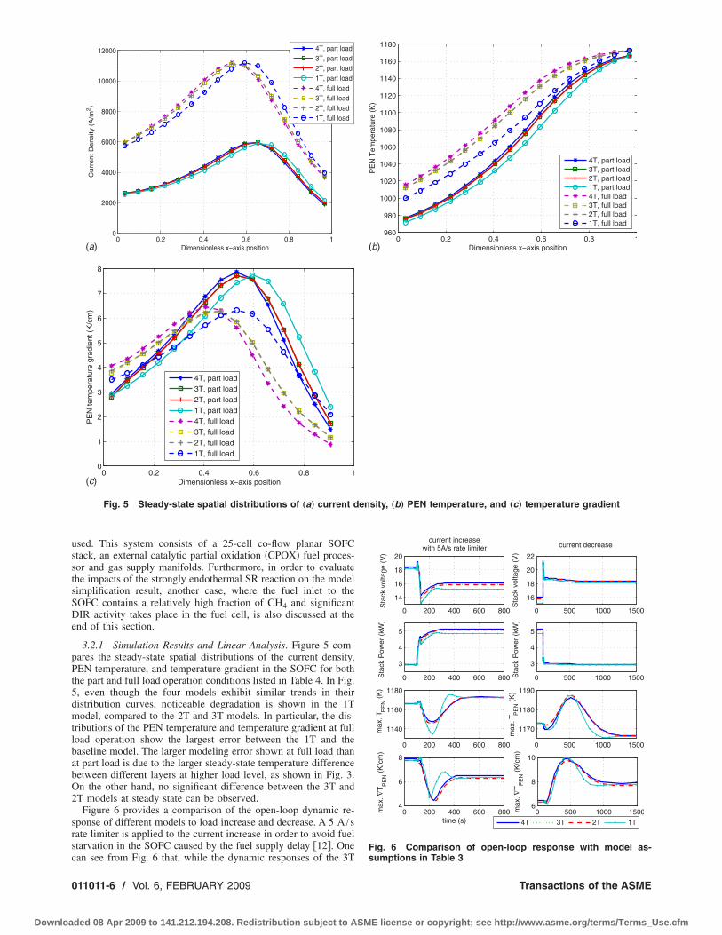
3.2.1 Simulation Results and Linear Analysis. Figure 5 com-ares the steady-state spatial distributions of the current density,EN temperature, and temperature gradient in the SOFC for both

he part and full load operation conditions listed in Table 4. In Fig., even though the four models exhibit similar trends in theiristribution curves, noticeable degradation is shown in the 1Todel, compared to the 2T and 3T models. In particular, the dis-

ributions of the PEN temperature and temperature gradient at fulload operation show the largest error between the 1T and theaseline model. The larger modeling error shown at full load thant part load is due to the larger steady-state temperature differenceetween different layers at higher load level, as shown in Fig. 3.n the other hand, no significant difference between the 3T andT models at steady state can be observed.

Figure 6 provides a comparison of the open-loop dynamic re-ponse of different models to load increase and decrease. A 5 A /sate limiter is applied to the current increase in order to avoid fueltarvation in the SOFC caused by the fuel supply delay �12�. One

0 0.2 0.4 0.6 0.8 10

2000

4000

6000

8000

10000

12000

Dimensionless x−axis position

Cu

rre

nt

De

nsi

ty(A

/m2)

4T, part load3T, part load2T, part load1T, part load4T, full load3T, full load2T, full load1T, full load

(a)

0 0.2 0.4 0.6 0.8 10

1

2

3

4

5

6

7

8


PE

Nte

mpe

ratu

regr

adie

nt(K

/cm

)


(c)

Fig. 5 Steady-state spatial distributions of „a… current d

0 0.2 0.4 0.6 0.8 1960

980

1000

1020

1040

1060

1080

1100

1120

1140

1160

1180


PE

NT

empe

ratu

re(K

)


(b)

ensity, „b… PEN temperature, and „c… temperature gradient

an see from Fig. 6 that, while the dynamic responses of the 3T

11011-6 / Vol. 6, FEBRUARY 2009


0 200 400 600 800

14

16

18

20

Sta

ckvo

ltage

(V)

current increasewith 5A/s rate limiter

0 200 400 600 800

3

4

5

Sta

ckP

ower

(kW

)

0 200 400 600 800

1140

1160

1180

max

.TP

EN

(K)

0 200 400 600 8004

6

8

max

.∇T

PE

N(K

/cm

)

time (s)

0 500 1000 1500

16

18

20

22

Sta

ckvo

ltage

(V)

current decrease

0 500 1000 1500

3

4

5

Sta

ckP

ower

(kW

)

0 500 1000 1500

1170

1180

1190

max

.TP

EN

(K)

0 500 1000 15006

8

10

max

.∇T

PE

N(K

/cm

)

time (s)4T 3T 2T 1T

Fig. 6 Comparison of open-loop response with model as-
sumptions in Table 3


aeapcm

c�cr�galqettm0dspTptcm

J

Downloa

nd 2T models match the baseline model fairly well, the 1T modelxhibits different transient behaviors for both the current increasend decrease cases, especially in the response of maximum tem-erature and temperature gradient in the PEN structure when theurrent load increases. The dynamic simulation results show al-ost identical transient response for the 3T and 2T models.The observations obtained based on simulations can also be

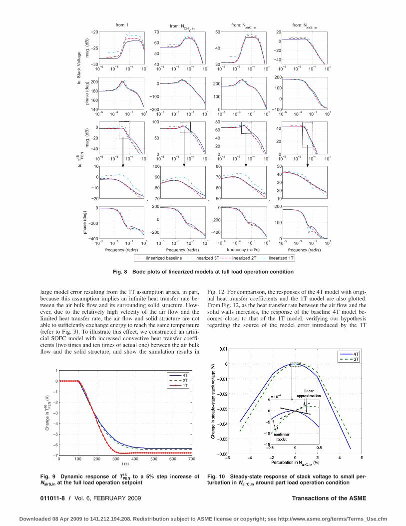
onfirmed by linear analysis. Figures 7 and 8 show the bode plots21� of the linearized models at the part and full load operationonditions, respectively. In these plots, we show the frequencyesponse of the stack voltage and maximum PEN temperatureTPEN

16 � to the system inputs, which include the total current �I� andas supply flow rates of CH4 �NCH4,in�, air to the CPOX �NairC,in�,nd air to the cathode �NairS,in�. As shown in Figs. 7 and 8, theinearized 1T model exhibits larger modeling error in the fre-uency response of TPEN

16 , compared to the 3T and 2T models. Forxample, as shown in Fig. 8, the 1T model has a higher bandwidthhan the other models in the response of TPEN

16 to NairS,in. In addi-ion, the decaying rate of the magnitude is much faster in the 1T

odel than the other models at the frequency about.01–0.1 rad /s, suggesting that the 1T model has higher orderynamics that do not exist in the other models. This is also con-istent with the simulation results shown in Fig. 9, which com-ares the transient response of the maximum PEN temperature,

PEN16 in the co-flow SOFC, for different models subject to a 5%erturbation in NairS,in at the full operation condition. One can seehat the 2T and 4T models have similar dynamic behaviors, whichan be approximated by a first-order dynamic system. The 1T

10−5 10−3 10−1 101−30

−25

−20from: I

mag.(dB)

10−5 10−3 10−1 101140

160

180

200

phase(deg)

10−5 10−3 10−140

50

60

70from: NCH

4, in

to:StackVoltage

10−5 10−3 10−1−200

0

200

400

10−5 10−3 10−1 101−40

−20

0

mag.(dB)

200

400

phase(deg)

10−5 10−3 10−10

50

100

to:T16 PEN

1000

1500

2000

10−5 10−3 10−1 1010

200

400

phase(deg)

frequency (rad/s)10−5 10−3 10−1

500

1000

1500

2000

frequency (rad/s

linearized baseline lin

−10

0

10

80

90

100

10−5 10−3 10−1 101140

160

180

200

10−5 10−3 10−1−200

−100

0

10−5 10−3 10−1 101−400

−200

0

phase(deg)

10−5 10−3 10−1−400

−200

0

200

Fig. 7 Bode plots of linearized mo

odel, however, exhibits quite different dynamics that correlate



with the higher order system response. From Figs. 7 and 8, it canalso be found that the linearized 3T and 2T models have almostthe same frequency response shown in these bode plots.

From Fig. 7, it is noted that the dc gain in the stack voltageresponse to NairC,in has different signs for the simplified modelsand the baseline model at the part load operation condition. This isdue to the system nonlinearity as well as the modeling errorcaused by combining the PEN and interconnector as one tempera-ture layer at this particular operating setpoint. Figure 10 comparesthe sensitivity of the steady-state stack voltage to small perturba-tions in NairC,in for the 4T and 3T models at the part load operationcondition. It can be found that, although the two curves exhibitsimilar trend in general, they have slopes with different signs atthe operation point, which accounts for the different sign of the dcgains in the linear analysis. Despite this difference of the dc gainsin linear analysis, the dynamic behavior of the 3T model is closeto that of the 4T model, as shown in Fig. 11 where the system issubject to 0.1% and 1% perturbations in NairC,in. From Fig. 11, onecan observe that the transient response of different models havesimilar characteristics. However, for the 0.1% perturbation case,the 4T model predicts a steady-state voltage decrease while the 3Tmodel predicts an increase, which is consistent with the linearanalysis results. Both models show steady-state voltage decreasewhen the perturbation is increased to 1%. Due to the small sensi-tivity of the voltage to NairC,in, this subtle difference does notresult in noticeable modeling error when the 4T model is reducedto the 3T and 2T models.

1

1

10−5 10−3 10−1 1010

20

40

60from: NairC, in

10−5 10−3 10−1 101200

400

600

800

10−5 10−3 10−1 101−40

−20

0

20from: NairS, in

10−5 10−3 10−1 101−200

0

200

1 10−5 10−3 10−1 10120

40

60

80

1000

1500

2000

10−5 10−3 10−1 1010

20

40

60

400

600

800

1000

1 10−5 10−3 10−1 101500

1000

1500

2000

frequency (rad/s)10−5 10−3 10−1 10

400

600

800

1000

frequency (rad/s)

zed 3T linearized 2T linearized 1T

50

60

70

80

30

40

50

1 10−5 10−3 10−1 101

0

200

400

10−5 10−3 10−1 101−100

0

100

200

1 10−5 10−3 10−1 101

−400

−200

0

10−5 10−3 10−1 1010

100

200

ls at part load operation condition

10

10

10

10)

eari

10

10

de

3.2.2 Reason for the Modeling Error in the 1T Model. The

FEBRUARY 2009, Vol. 6 / 011011-7


lbtela�ccfl

FN

0

Downloa

arge model error resulting from the 1T assumption arises, in part,ecause this assumption implies an infinite heat transfer rate be-ween the air bulk flow and its surrounding solid structure. How-ver, due to the relatively high velocity of the air flow and theimited heat transfer rate, the air flow and solid structure are notble to sufficiently exchange energy to reach the same temperaturerefer to Fig. 3�. To illustrate this effect, we constructed an artifi-ial SOFC model with increased convective heat transfer coeffi-ients �two times and ten times of actual one� between the air bulkow and the solid structure, and show the simulation results in

10−5 10−3 10−1 101−30

−25

−20

from: I

mag.(dB)

10−5 10−3 10−1 101140

160

180

200phase(deg)

10−5 10−3 10−140

50

60

70from: NCH

4, in

to:StackVoltage

10−5 10−3 10−1−200

0

200

400

10−5 10−3 10−1 101

−40

−20

0

mag.(dB)

200

400

600

800

phase(deg)

10−5 10−3 10−10

50

100

to:T16 PEN

1000

2000

10−5 10−3 10−1 1010

200

400

600

800

phase(deg)

frequency (rad/s)10−5 10−3 10−10

1000

2000

frequency (rad/s)

linearized baseline line

−1−20

−10

0

10

70

80

90

100

10−5 10−3 10−1 101140

160

180

200phase(deg)

10−5 10−3 10−1−200

−100

0

10−5 10−3 10−1 101−400

−200

0

phase(deg)

10−5 10−3 10−1

−200

0

200

Fig. 8 Bode plots of linearized m

0 100 200 300 400 500 600 700−7

−6

−5

−4

−3

−2

−1

0

1

t (s)

Cha

nge

inT16 P

EN

(K)

4T2T1T

ig. 9 Dynamic response of TPEN16 to a 5% step increase of

airS,in at the full load operation setpoint

11011-8 / Vol. 6, FEBRUARY 2009


Fig. 12. For comparison, the responses of the 4T model with origi-nal heat transfer coefficients and the 1T model are also plotted.From Fig. 12, as the heat transfer rate between the air flow and thesolid walls increases, the response of the baseline 4T model be-comes closer to that of the 1T model, verifying our hypothesisregarding the source of the model error introduced by the 1T

10−5 10−3 10−1 10130

40

50from: NairC, in

10−5 10−3 10−1 101400

500

600

10−5 10−3 10−1 101−40

−20

0

20from: NairS, in

10−5 10−3 10−1 101−100

0

100

200

10−5 10−3 10−1 1010

20

40

60

80

1500

2000

2500

10−5 10−3 10−1 1010

20

40

500

1000

1500

10−5 10−3 10−1 1011000

1500

2000

2500

frequency (rad/s)10−5 10−3 10−1 1010

500

1000

1500

frequency (rad/s)

ed 3T linearized 2T linearized 1T

1 −150

60

70

80

−10

20

30

40

50

10−5 10−3 10−1 1010

100

200

10−5 10−3 10−1 101−100

0

100

200

10−5 10−3 10−1 101

−400

−200

0

10−5 10−3 10−1 1010

100

200

ls at full load operation condition

Fig. 10 Steady-state response of stack voltage to small per-

101

101

101

101

ariz

−

101

101

ode

turbation in NairC,in around part load operation condition



aomc

iTasalctFisraadet

Iwfic

Ft

Fs

J

Downloa

ssumption. The relatively larger model error observed in the casef current increase shown in Fig. 6 can also be explained since theodel error caused by the 1T assumption becomes more signifi-

ant with faster air flow velocity at high load.Compared to the air flow, the fuel flow has much lower veloc-

ty. For example, at the part load operation condition given inable 4, the fuel flow velocity is about 1.5 m /s and the air flowbout 10.5 m /s. The difference between the fuel and air flowpeeds is even larger at full load operation �about 3.3 m /s versusbout 30 m /s� because of the higher air excess ratio used at fulload operation. At these speeds, the fuel flow can conduct suffi-ient heat transfer with the solid structure, resulting in a similaremperature response in the fuel flow and solid parts, as shown inig. 3. Therefore, combining the fuel bulk flow and solid structure

nto one temperature layer, as in the 2T model, does not introduceignificant error for our system. Figure 13 compares simulationesults when the heat transfer coefficient between the fuel flownd the solid structure is intentionally decreased �5% and 0.5% ofctual one� in the baseline model. As this heat transfer coefficientecreases, the 2T assumption would cause a larger model error,specially in the dynamic response of the maximum PENemperature.

3.2.3 Effects of Low Fuel Utilization and Fast Currentncrease. Figure 14 shows the simulation results of the systemith the same operating parameters in Table 4, except that a lower

uel utilization ratio �50%� is used. The rate limiter of currentncrease is set at 20 A /s in this case to allow a more rapid in-rease in the current load during transient. While the 1T model

0 500 1000 1500−6

−5

−4

−3

−2

−1

0

1x 10

−3

t (s)

chan

gein

stac

kvo

ltage

(V)

0.1% purturbation in NairC, in

0 500 1000 1500−0.06

−0.05

−0.04

−0.03

−0.02

−0.01

0

0.01

t (s)

chan

gein

stac

kvo

ltage

(V)

1% purturbation in NairC, in

4T3T

4T3T

ig. 11 Dynamic response of stack voltage to small perturba-ion in NairC,in around part load operation condition

0 200 400 600 800

14

16

18

20

Sta

ckvo

ltage

(V)

0 200 400 600 800

3

4

5

Sta

ckP

ower

(kW

)

4T 4T, 2ka

4T, 10ka 1T

0 200 400 600 800

1140

1160

1180

max

.TP

EN

(K)

time (s)0 200 400 600 800

4

6

8

max

.∇T

PE

N(K

)

time (s)

ig. 12 Effects of heat transfer rates between air flow and
olid structure on open-loop response to load increase


leads to significant model error, the 2T and 3T models are stillconsistent with the baseline model in dynamic response, espe-cially considering the trend in slow dynamics. Compared to thesimulation results plotted in Fig. 6, larger differences in the re-sponse of the maximum PEN temperature can be observed be-tween the 2T/3T and baseline models in Fig. 14 during the shortperiod right after the current load is increased. This is because thelower fuel utilization ratios result in a higher current density in thelast unit, which corresponds to the highest PEN temperature in theco-flow SOFC. With more rapid current increases, more heat isgenerated in the PEN structure of the last unit and accumulatedhere due to the finite, albeit fast, heat transfer rate between thePEN assembly and the other layers. Nevertheless, as shown inFig. 14, the trend in the dynamic response of the 2T model stillretains the main characteristics of the baseline model fairly well.Considering practical constraints such as actuator saturations anddynamics in parasitic devices, the current increase in the last unitduring transients will be very limited in normal operations. Thus,the error introduced by combining the PEN and interconnectorinto one temperature layer can be expected to be negligible for ourapplications.

As revealed by the above analysis, the 2T assumption, i.e., as-

0 200 400 600 800

14

16

18

20

Sta

ckvo

ltage

(V)

0 200 400 600 8003

4

5

Sta

ckP

ower

(kW

)

4T 4T, 0.05kf

4T, 0.005kf 2T

0 200 400 600 800

1150

1160

1170

max

.TP

EN

(K)

time (s)0 200 400 600 800

4

6

8

max

.∇T

PE

N(K

)

time (s)

Fig. 13 Effects of heat transfer rates between fuel flow andsolid structure on open-loop response to load increase

0 200 400 600 80014

16

18

20

Sta

ckvo

ltage

(V)


0 200 400 600 800

3

4

5

6

Sta

ckP

ower

(kW

)

0 200 400 600 800

1120

1140

1160

max

.TP

EN

(K)

0 200 400 600 800

4

6

8

max

.∇T

PE

N(K

/cm

)

time (s)

0 500 1000 150016

18

20

22

Sta

ckvo

ltage

(V)

current decrease

0 500 1000 1500

3

4

5

6

Sta

ckP

ower

(kW

)

0 500 1000 1500

1120

1140

1160

max

.TP

EN

(K)

0 500 1000 1500

6

8

10

max

.∇T

PE

N(K

/cm

)

time (s)4T 3T 2T 1T

Fig. 14 Comparison of open-loop response with model as-
sumptions in Table 3. Fuel utilization ratio=50%.
FEBRUARY 2009, Vol. 6 / 011011-9


sstsmmpM

tcwsc12

M

a

0

Downloa

uming two temperature layers �the air bulk flow and the solidtructure� in the energy balance, represents a good trade-off be-ween model accuracy and complexity. In this simplification, twotates in each discretization unit are removed from the baselineodel while the key dynamic characteristics are preserved. Thisodel simplification also results in a significant reduction in com-

utation time, as shown in Table 5. All the models are built inATLAB/SIMULINK. The CPU time reported is the average of three

imes the simulations considered in Fig. 6, with the current in-rease from part to full load. All simulations are run on a desktopith a Pentium4 3.2 GHz CPU and 504 Mbyte memory. As

hown in Table 5, the 2T model can save about 40% CPU time,ompared to the baseline model. It is also noted, however, that theT model imposes even more computation burden than the 3T andT ones do, and the reason needs to be investigated.

Table 5 Comparison of computation efficiency

odelNumber of states in each

discretization unitNumber of states in

SOFC modela CPU time �s�

4T 12 192 5223T 11 176 3352T 10 160 3161T 9 144 360

Based on the 16-unit discretization scheme.

0 0.2 0.4 0.6 0.8 12000

4000

6000

8000

10000

12000

14000


Cur

rent

Den

sity

(A/m

2 )


(a)

0 0.2 0.4 0.6 0.8 1−4

−2

0

2

4

6

8


PE

Nte

mpe

ratu

regr

adie

nt(K

/cm

)


(c)

Fig. 15 Steady-state spatial distributions of „a… current den
ating setpoints given in Table 6 are used for simulations
11011-10 / Vol. 6, FEBRUARY 2009


3.3 Impacts of Direct Internal Reforming on Performanceof Simplified Model. Reforming methane through SR and WGSreactions inside the fuel channel of SOFCs, as shown in Fig. 1, iscalled DIR and has the potential to reduce the size of the externalreformer and improve system efficiency �1�. As shown in Sec. 2,DIR has been incorporated in the baseline model. Note that SR isa strongly endothermal reaction ��H0=206 kJ /mol�; DIR couldhave significant influence on the spatial distribution and dynamicresponse of the SOFC, and therefore its impacts on model simpli-fication results need to be analyzed.

For SOFC systems fed with fuels processed by the CPOX re-former, however, the amount of CH4 remaining in the reformate isrelatively small �less than 2% in molar fraction for the operationconditions given in Table 4�, which leads to insignificant steamreforming activity inside the SOFC. In order to investigate theeffects of DIR on the performance of the SOFC models withsimplified energy balance dynamics, it is assumed in the followingthat the fuel fed to the SOFC is reformed through an external SRpre-reformer with a specified pre-reforming ratio. The pre-reforming ratio is defined as the fraction of CH4 processed in thereformer over the total amount of fuel entering the reformer. MoreCH4 will remain in the reformate at lower pre-reforming ratio andreacts through the DIR inside the fuel channel of the SOFC.

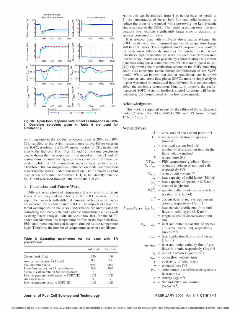
Steady-state simulation results using models with different tem-perature layer assumptions in this case are compared in Fig. 15,while Fig. 16 compares dynamic responses of these models. Theoperation parameters listed in Table 6 are used, where the pre-

0 0.2 0.4 0.6 0.8 1960

980

1000

1020

1040

1060

1080

1100

1120

1140

1160

1180


PE

NT

empe

ratu

re(K

)


(b)

, „b… PEN temperature, and „c… temperature gradient. Oper-
sity


rCticamTreS

4

lpafcauPl

F3s

Tp

C

AFPSIAI

J

Downloa

eforming ratio in the SR fuel processor is set at 20%, i.e., 80%H4 supplied to the system remains unreformed before entering

he SOFC, resulting in a 23.5% molar fraction of CH4 in the fuelnlet to the fuel cell. From Figs. 15 and 16, the same conclusionan be drawn that the responses of the model with the 2T and 3Tssumptions resemble the dynamic characteristics of the baselineodel, while the 1T assumption induces large model errors.herefore, DIR has insignificant influence on model simplification

esults for the system under consideration. The 2T model is validven when substantial unreformed CH4 is fed directly into theOFC and reformed through DIR inside the fuel cell.

Conclusion and Future WorkDifferent assumptions of temperature layers result in different

evels of accuracy and complexity in the SOFC models. In thisaper, four models with different numbers of temperature layersre explored for co-flow planar SOFCs. The impacts of these dif-erent assumptions on the model performance are investigated byomparing the steady-state and dynamic simulation results as wells using linear analysis. Our analyses show that, for the SOFCnder consideration, the temperature profiles in the fuel bulk flow,EN, and interconnector can be approximated as one temperature

ayer. Therefore, the number of temperature states in each discreti-

0 200 400 600 80012

14

16

18

20

Sta

ckvo

ltage

(V)


0 200 400 600 800

3

4

5

Sta

ckP

ower

(kW

)

0 200 400 600 800

1120

1140

1160

max

.TP

EN

(K)

0 200 400 600 8004

6

8

10

max

.|∇

TP

EN

|(K

/cm

)

time (s)

0 500 1000 150012

14

16

18

20

Sta

ckvo

ltage

(V)

current decrease

0 500 1000 1500

3

4

5

Sta

ckP

ower

(kW

)

0 500 1000 1500

1120

1140

1160

max

.TP

EN

(K)

0 500 1000 15004

6

8

10

max

.|∇

TP

EN

|(K

/cm

)

time (s)

4T 3T 2T 1T

ig. 16 Open-loop response with model assumptions in Table. Operating setpoints given in Table 6 are used forimulations.

able 6 Operating parameters for the case with SRre-reformer

Full load Part load

urrent load, I �A� 320 160

ve. current density, i �A /cm2� 0.8 0.4

uel utilization ratio 90% 90%re-reforming ratio in SR pre-reformer 20% 20%team-to-carbon ratio in SR pre-reformer 2 2nlet temperature of reformate to SOFC �K� 1023 1023ir excess ratio 9 7

nlet temperature of air to SOFC �K� 1023 1023



zation unit can be reduced from 4 as in the baseline model to2—the temperatures of the air bulk flow and solid structure—toreduce the order of the model while preserving the key dynamiccharacteristics of the SOFC. The model assuming only one tem-perature layer exhibits significantly larger error in dynamic re-sponses compared to others.

It is noticed that, with a 16-unit discretization scheme, theSOFC model with the minimized number of temperature layersstill has 160 states. The simplified model proposed here containsthe same mass balance dynamics as the baseline model, whichintroduces eight concentration states for each discretization unit.Further model reduction is possible by approximating the gas flowdynamics using quasi-static relations, which is investigated in Ref.�19�. Optimizing the discretization scheme in the SOFC modelingcould also contribute to the further simplification of the SOFCmodel. While we believe that similar conclusions can be drawnfor counter- and cross-flow planar SOFCs, more in-depth analysisis also warranted to understand how different flow pattern mightaffect the modeling assumption. Finally, to improve the perfor-mance of SOFC systems, feedback control solutions will be de-veloped in the future, based on the low-order model.

AcknowledgmentThis work is supported in part by the Office of Naval Research

under Contract No. N00014-06-1-0209 and US Army throughTCN05158�SSP�.

NomenclatureA cross area of the current path �m2�

Cs molar concentration of species s�mol /m3�

I electrical current load �A�J number of discretization units in the

finite volume methodT temperature �K�

�TPEN PEN temperature gradient �K/cm�U, Ucell operating voltage of unit and cell,

respectively �V�UOCV open circuit voltage �V�

cp heat capacity of solid layers �J/K kg�cv,s heat capacity of species s �J/K mol�

d channel height �m�hs�T� specific enthalpy of species s at tem-

perature of T �J/mol�i, i current density and average current

density, respectively �A /m2�kf ,PEN, ka,PEN, kf ,I, ka,I heat transfer coefficients from bulk

flows to solid layers �J /K m2 s�l length of spatial discretization unit

�m�nin,s, nout,s inlet and outlet molar flux of species

s in a volumetric unit, respectively�mol /s m2�

qcond heat conduction flux in solid layers�J /s m2�

qin, qout inlet and outlet enthalpy flux of gasflows in a unit, respectively �J /s m2�

rk rate of reaction k �mol /s m2�uout outlet flow velocity �m/s�

� emissivity of solid layers� potential loss �V�

�s,k stoichiometric coefficient of species sin reaction k

� density �kg /m3�� Stefan-Boltzmann constant

2 4
�W /m K �
FEBRUARY 2009, Vol. 6 / 011011-11


S

S

R

0

Downloa

� solid layer thickness �m�

ubscriptI interconnector

ox oxidation reactionred reduction reaction

a air flowf fuel flow

sa species in the air flowsf species in the fuel flow

sol solid structure in SOFC

uperscriptj the jth discretization unit

eferences�1� Singhal, S. C., and Kendall, K., eds., 2004, High Temperature Solid Oxide

Fuel Cells: Fundamentals, Design and Applications, Elsevier Science, NewYork.

�2� Achenbach, E., 1994, “Three-Dimensional and Time-Dependent Simulation ofa Planar Solid Fuel Cell Stack,” J. Power Sources, 49, pp. 333–348.

�3� Braun, R. J., 2002, “Optimal Design and Operation of Solid Oxide Fuel CellSystems for Small-Scale Stationary Applications,” Doctoral thesis, Universityof Wisconsin-Madison, Madison, WI.

�4� Petruzzi, L., Cocchi, S., and Fineschi, F., 2003, “A Global Thermo-Electrochemical Model for SOFC Systems Design and Engineering,” J. PowerSources, 118, pp. 96–107.

�5� Aguiar, P., Adjiman, C. S., and Brandon, N. P., 2004, “Anode-Supported In-termediate Temperature Direct Internal Reforming Solid Oxide Fuel Cell. I:Model-Based Steady-State Performance,” J. Power Sources, 138, pp. 120–136.

�6� Gemmen, R. S., and Johnson, C. D., 2005, “Effect of Load Transients onSOFC Operation-Current Reversal on Loss of Load,” J. Power Sources, 144,pp. 152–164.

�7� Sedghisigarchi, K., and Feliachi, A., 2004, “Dynamic and Transient Analysisof Power Distribution Systems With Fuel Cells-Part I: Fuel Cell DynamicModel,” IEEE Trans. Energy Convers., 19, pp. 423–428.

�8� Xi, H., and Sun, J., 2005, “Dynamic Model of Planar Solid Oxide Fuel Cells
for Steady State and Transient Performance Analysis,” Proceedings of ASME
11011-12 / Vol. 6, FEBRUARY 2009


International Mechanical Engineering Congress and Exposition, Orlando, FL,Nov. 5–11.

�9� Sorrentino, M., Guezennec, Y. G., Pianese, C., and Rizzoni, G., 2005, “Devel-opment of a Control-Oriented Model for Simulation of SOFC-Based EnergySystems,” Proceedings of ASME International Mechanical Engineering Con-gress and Exposition, Orlando, FL, Nov. 5–11.

�10� Achenbach, E., 1995, “Response of a Solid Oxide Fuel Cell to Load Change,”J. Power Sources, 57, pp. 105–109.

�11� Aguiar, P., Adjiman, C. S., and Brandon, N. P., 2005, “Anode-Supported In-termediate Temperature Direct Internal Reforming Solid Oxide Fuel Cell. II:Model-Based Dynamic Performance and Control,” J. Power Sources, 147, pp.136–147.

�12� Xi, H., and Sun, J., 2006, “Analysis and Feedback Control of Planar SOFCSystems for Fast Load Following in APU Applications,” Proceedings of ASMEInternational Mechanical Engineering Congress and Exposition, Chicago, IL,Nov. 5–10.

�13� Campanari, S., and Iora, P., 2005, “Comparison of Finite Volume SOFC Mod-els for the Simulation of a Planar Cell Geometry,” Fuel Cells, 5�1�, pp. 34–51.

�14� Xi, H., and Sun, J., 2006, “Comparison of Dynamic Planar SOFC Models WithDifferent Assumptions of Temperature Layers in Energy Balance,” Proceed-ings of ASME International Mechanical Engineering Congress and Exposition,Chicago, IL, Nov. 5–10.

�15� Iora, P., Aguiar, P., Adjiman, C. S., and Brandon, N. P., 2005, “Comparison ofTwo IT DIR-SOFC Models: Impact of Variable Thermodynamic, Physical, andFlow Properties. Steady-State and Dynamic Analysis,” Chem. Eng. Sci., 60,pp. 2963–2975.

�16� Mueller, F., Brouwer, J., Jabbari, F., and Samuelsen, S., 2006, “DynamicSimulation of an Integrated Solid Oxide Fuel Cell System Including Current-Based Fuel Flow Control,” ASME J. Fuel Cell Sci. Technol., 3, pp. 144–154.

�17� Ota, T., Koyama, M., Wen, C., Yamada, K., and Takahashi, H., 2003, “Object-Based Modeling of SOFC System: Dynamic Behavior of Micro-Tube SOFC,”J. Power Sources , 118, pp. 430–439.

�18� Larminie, J., and Dicks, A., 2003, Fuel Cell Systems Explained, 2nd ed.,Wiley, New York.

�19� Xi, H., and Sun, J., 2007, “A Low Order Dynamic Model for Planar SolidOxide Fuel Cells Using On-Line Iterative Computation,” ASME J. Fuel CellSci. Technol., to be published.

�20� Selimovic, A., 2002, “Modeling of Solid Oxide Fuel Cells Applied to theAnalysis of Integrated Systems With Gas Turbines,” Doctoral thesis, LundUniversity, Sweden.

�21� Franklin, G. F., Powell, J. D., and Emami-Naeini, A., 2002, Feedback Control
of Dynamic Systems, 4th ed., Prentice-Hall, Englewood Cliffs, NJ.


Date post:	07-Apr-2020
Category:	Documents
Upload:	others
View:	7 times
Download:	0 times

Dynamic Analysis of Planar Solid Oxide Fuel Cell Models...

Documents