Abstract A new semi-analytical approach to analyze the dynamic response of railway bridges subjected tohigh-speed trains is presented. The bridge is modeled as an Euler–Bernoulli beam on viscoelastic supportsthat account for the flexibility and damping of the underlying soil. The track is represented by an Euler–Bernoulli beamon viscoelastic bedding. Complexmodal expansion of the bridge and trackmodels is performedconsidering non-classical damping, and coupling of the two subsystems is achieved by component modesynthesis (CMS). The resulting system of equations is coupled with a moving mass–spring–damper (MSD)system of the passing train using a discrete substructuring technique (DST). To validate the presentedmodelingapproach, its results are compared with those of a finite element model. In an application, the influence of thesoil–structure interaction, the track subsystem, and geometric imperfections due to track irregularities on thedynamic response of an example bridge is demonstrated.
1 Introduction
In the last two decades, the importance of the dynamics of railway bridges has grown considerably due to theincreased development of high-speed railway lines. In fact, at high, so-called critical train speeds, resonancephenomena occur more frequently in bridge structures, resulting from excitation by the moving axle loads atconstant spacing, as well as from track irregularities and wheel hunting movements. Resonance phenomenain railway bridges usually do not lead to a loss of load-bearing capacity, but to the exceeding of the maximumallowable accelerations of the bridge deck. In such cases, the ballast bed becomes instable, reducing themaintenance intervals for the track or requiring a reduction in train speed. In catastrophic conditions, thechange in track position may even lead to train derailments. The numerical prediction of the dynamic responseof railway bridges is therefore of great importance.
First studies on the dynamic behavior of railway bridges date back to the nineteenth century (e.g., [32,38]),as described in the comprehensive overview of early contributions in [16]. The simplest approaches dealing
P. König · P. Salcher · C. Adam (B) · B. HirzingerUnit of Applied Mechanics, University of Innsbruck, Technikerstr. 13, 6020 Innsbruck, AustriaE-mail: [email protected]
with these problems include the modeling of the bridge as a beam-like structure subjected to moving singleloads, which correspond to the axle loads of the train [13,17,36]. In more complex models, the bridge isrepresented by a 3D finite element (FE) model and the train as a 3D mass–spring–damper (MSD) system [40]in which rigid bodies are connected by lumped spring–damper elements [31,46]. To determine the dynamicresponse of the coupled system, in a classical approach, both subsystems are first treated individually andthen coupled via a coupling condition at the point of contact [45]. However, these models can only be createdwith great effort and do not allow parameter studies or stochastic simulations. The simplest model approachto explicitly consider the dynamic interaction between train and bridge consists of a beam for the bridge anda plane MSD system for the train [41,44]. These, as well as other simplifying models (e.g., [10] and [22]),are suitable for computationally intensive investigations of the failure probability of railway bridges usingstochastic simulations [21]. In these simplified beam models, the track is not explicitly modeled. An exceptionis the model presented in [3], where the track is represented as an additional beam, which rests on viscoelasticbedding on the bridge and the adjacent areas to be connected. For the coupling of the subsystems of the bridgebeam and track beam, the authors of [3] used a variant of the so-called component mode synthesis (CMS).
A recent contribution on vehicle–bridge interaction [33] proposed a method to decouple the vehicle–bridgeinteraction problem, taking the influence of the traversing vehicle on the natural frequencies and damping ofthe bridge [34] into account. Other recent studies have shown that the soil–structure interaction can have asignificant impact on the prediction of the dynamic bridge response [5,35,37,42]. Discretization of the half-space and foundations by means of finite elements or boundary elements [18,30,37] leads to a computationaleffort that is hardly feasible. Alternatively, the soil can be represented in a simplifiedmanner by spring–damperelements below the bridge supports [11,39]. In a recent paper [20], such a beammodel on viscoelastic supportscrossed by a movingMSD system was developed. The solution of this coupled non-classically damped systemwas found by means of a dynamic substructuring technique (DST), and the approach of the MSD system atthe beam and its departure after crossing the beam were approximated by simplifying assumptions.
The aim of the present contribution is to extend this non-classically damped model of the bridge beam [20]by a track on viscoelastic bedding. The CMS approach for simply supported single-span beams presented in[3] serves as a basis for considering the track substructure as a separate beam. The proposed model is thusable to capture the load distribution by the track on the bridge structure. Consequently, there is no need forsimplified assumptions for the approach and departure conditions of the train, as described in [20]. In addition,track irregularities are accounted for by appropriate irregularity profile functions [8]. This way, the proposedmodel captures the dynamic train–track–bridge–soil interaction including track irregularities and provides asolid basis for further numerical investigations.
In the present paper, first the models and the corresponding equations of motion of the individual subsys-tems, track, bridge–soil, and train, are described. A modal expansion of the soil–bridge and track subsystemsis performed, and the coupling of the subsystem is achieved using CMS [2,3]. This set of equations is thencoupled with the MSD system of the train using a DST and subsequently solved numerically. In order tovalidate the proposed model, a numerical study is carried out comparing the results of the presented methodwith those of a finite element model. Further numerical investigations include the comparison of the responsewith and without track substructure and the results with and without soil–structure interaction, with aspectsof each subsystem discussed. Finally, some important findings on the consideration of rail irregularities arepresented.
2 Modeling of the train–track–bridge–soil system
For the present investigations, the interaction system consisting of the high-speed train moving at constantspeed v, the track, the bridge with foundation, and the soil is modeled as a plane system, which is shownin Fig. 1. The rails and the slender bridge are both modeled as Euler–Bernoulli beams with constant cross-section. The rail system on top of the bridge is resting on a viscoelastic Winkler bedding, which representsthe mechanical properties of the track and the underlying subgrade. Rail irregularities are taken into accountby introducing random irregularity profile functions on the rail beam surface [8], which describe the deviationfrom a perfectly smooth track. The viscoelastic bearings at both ends of the bridge beam represent the stiffnessand damping of the supporting soil. To account for themass of the foundation and the soil above the foundation,lumped masses at each end of the bridge are added. It is assumed that a conventional train composed of Ncindividual vehicles crosses the bridge. Each vehicle, which consists of a car body, two bogies, and four axles,is modeled as a mass–spring–damper (MSD) system with ten degrees of freedom (DOFs).
Dynamic analysis of railway bridges 4585
Fig. 1 Viscoelastically supported single-span bridge model with track crossed by a planar MSD model, which represents the j thtrain vehicle
3 Equations of motion and boundary conditions
The interacting system shown in Fig. 1 is at first split into the subsystems of the track, the bridge–soil, and thetrain. In this Section, the equations of motions of each subsystem are presented.
3.1 Track subsystem
The Euler–Bernoulli beam with the length L r, which represents the track substructure, has a constant mass perunit length ρAr and a constant flexural rigidity E Ir and rests on a viscoelastic Winkler bedding with stiffnesscoefficient kf(x) and damping coefficient cf(x). The bedding parameters can be different in the bridge section(then denoted as kfb and cfb) and in the area of the subsoil (then denoted as kf0 and cf0). The origin of the axialcoordinate x = 0 is located at the left viscoelastic bridge bearing. In the model, the theoretically infinitelylong track superstructure is considered to be simply supported at both ends. To ensure that the effects of these“artificially” introduced boundary conditions on the system response at the bridge are negligible, the track inthe model must have the following minimum length before and after the bridge [3,12]:
L0 ≥ 2π 4
√4E Irkf0
. (1)
The deflection wr(x, t) of the track model is governed by the following equation of motion [9]:
The distributed force qr(x, t) results from the viscoelastic bedding counteracting the displacement of the track,
qr(x, t) =kf(x) (wr(x, t) − wb(x, t)� (x, 0, Lb))
+ cf(x) (wr(x, t) − wb(x, t)�(x, 0, Lb)) ,(3)
4586 P. König et al.
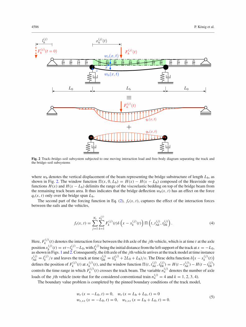
Fig. 2 Track–bridge–soil subsystem subjected to one moving interaction load and free-body diagram separating the track andthe bridge–soil subsystems
where wb denotes the vertical displacement of the beam representing the bridge substructure of length Lb, asshown in Fig. 2. The window function �(x, 0, Lb) = H(x) − H(x − Lb) composed of the Heaviside stepfunctions H(x) and H(x − Lb) delimits the range of the viscoelastic bedding on top of the bridge beam fromthe remaining track beam area. It thus indicates that the bridge deflection wb(x, t) has an effect on the forceqr(x, t) only over the bridge span Lb.
The second part of the forcing function in Eq. (2), fr(x, t), captures the effect of the interaction forcesbetween the rails and the vehicles,
fr(x, t) =Nc∑j=1
n( j)a∑
k=1
F ( j)k (t)δ
(x − x ( j)
k (t))
�(t, t ( j)Ak , t ( j)Dk
). (4)
Here, F ( j)k (t) denotes the interaction force between the kth axle of the j th vehicle, which is at time t at the axle
position x ( j)k (t) = vt−l( j)k −L0,with l
( j)k being the initial distance from the left support of the track at x = −L0,
as shown in Figs. 1 and 2. Consequently, the kth axle of the j th vehicle arrives at the trackmodel at time instancet ( j)Ak = l( j)k /v and leaves the track at time t ( j)Dk = (l( j)k + 2L0 + Lb)/v. The Dirac delta function δ
(x − x ( j)
k (t))
defines the position of F ( j)k (t) at x ( j)
k (t), and the window function �(t, t ( j)Ak , t ( j)Dk ) = H(t − t ( j)Ak )− H(t − t ( j)Dk )
controls the time range in which F ( j)k (t) crosses the track beam. The variable n( j)
a denotes the number of axle
loads of the j th vehicle (note that for the considered conventional train n( j)a = 4 and k = 1, 2, 3, 4).
The boundary value problem is completed by the pinned boundary conditions of the track model,
The half-space (soil) below the vertically excited rigid bridge foundations is represented in a simplifiedmannerby spring–damper elements [11] located below the bridge bearings, as shown in Fig. 1. Assuming that thehalf-space is homogeneous, the spring stiffness kb and the viscous damping parameter cb of these elementscan be estimated, for instance, based on the Wolf cone model [39],
kb = ρsc2wA0
z0, cb = ρscwA0, (6)
where
z0 = π
4(1 − ν)
(cwcs
)2
r0. (7)
ρs is the density of the soil, A0 the contact area of the foundation, r0 = √A0/π the equivalent radius of a
circular plate with the same area as the foundation, and cs = √G/ρs the shear velocity with G denoting the
shear modulus of the soil. Depending on Poisson’s ratio ν of the subsoil, the variable cw is either equal to thecompression wave velocity cp or twice the shear wave velocity cs of the homogeneous half-space,
cw =⎧⎨⎩cp =
√Esρs
ν ≤ 1/3
2cs = 2√
Gρs
1/3 < ν ≤ 1/2, (8)
with the constrained modulus Es of soil, which is related to the shear modulusG by Es = 2G(1−ν)/(1−2ν).The dynamic stiffness decreases with increasing frequency, but since the stiffness coefficient kb is a staticquantity, for soils with a Poisson’s ratio ν > 1/3, additionally the lumped mass mg must be considered [39],
mg = 2.4√π
(ν − 1
3
)ρsA
(3/2)0 . (9)
The lumped mass mb located at both bridge bearings represents thus the mass of the bridge foundationsm1, the mass of the soil above the foundations m2, and the lumped soil mass mg, i.e., mb = m1 + m2 + mg.
The vertical displacementwb(x, t) of the Euler–Bernoulli beamwith constant mass per unit length ρAb andconstant flexural rigidity E Ib satisfies the following partial differential equation [9] in the range 0 ≤ x ≤ Lb:
is the force that is transferred to the bridge via the viscoelastic Winkler bedding, as shown in Fig. 2. Thecorresponding boundary conditions of the present beam problem are [20]
The planar model of the j th vehicle of the considered conventional train is composed of seven rigid bodieswith mass, i.e., the car body (subscript “p”), two bogies (subscript “s”), and four axles (subscript “a”), whichare connected by spring–damper elements, as shown in Fig. 1. The model with a total of 10 DOFs has threerotational DOFs (rotation of the car body ϕ
( j)p and of the bogies ϕ
( j)s1 and ϕ
( j)s2 ) and seven translational DOFs
(vertical axle displacements u( j)a1 , u
( j)a2 , u
( j)a3 , u
( j)a4 ; vertical displacement of the center of gravity of the car body
4588 P. König et al.
u( j)p ; vertical displacement of the center of gravity of the bogies u( j)
s1 , u( j)s2 ) [23,27], which are combined in the
vector u( j)c ,
u( j)c =
[u( j)p , ϕ( j)
p , u( j)s1 , ϕ
( j)s1 , u( j)
s2 , ϕ( j)s2 , u( j)
a1 , u( j)a2 , u( j)
a3 , u( j)a4
]T. (13)
Neglecting the horizontal interaction between the Nc individual vehicles, the combined equations ofmotionof the complete train can be written as [31]
Mcuc + Ccuc + Kcuc = Fc, (14)
withMc, Cc, andKc being the mass, damping, and stiffness matrices of the train resulting from the individualsystem matrices of each vehicle,
Mc = diag[M(1)
c , . . . ,M( j)c , . . . ,M(Nc)
c
],
Cc = diag[C(1)c , . . . ,C( j)
c , . . . ,C(Nc)c
],
Kc = diag[K(1)
c , . . . ,K( j)c , . . . ,K(Nc)
c
],
uc =[u(1)c , . . . ,u( j)
c , . . . ,u(Nc)c
]T. (15)
The vehicle system matrices M( j)c ,C( j)
c ,K( j)c can be found in [20,31]. The force vector
Fc =[F(1)c ,F(2)
c , . . . ,F(Nc)c
]T(16)
is composed of the individual interaction force vectors (Fig. 1)
F( j)c =
[0, 0, 0, 0, 0, 0, F ( j)
as + F ( j)a1 , F ( j)
as + F ( j)a2 , F ( j)
as + F ( j)a3 , F ( j)
as + F ( j)a4
]T(17)
between the vehicle and the rail substructures at the position of each axle of the Nc vehicles. Each interactionforce in turn consists of a dynamic component, F ( j)
ak (k = 1, . . . , 4), and a static component F ( j)as ,
F ( j)as = g
4
(m( j)
p + 2m( j)s + 4m( j)
a
), (18)
which is simply the gravity load of the vehicle distributed over the four axles, with g denoting the accelerationof gravity. In state space, the equations of motion of the train (Eq. 15) become [20]
Acdc + Bcdc = fc, (19)
with
Ac =[Cc McMc 0
], Bc =
[Kc 00 −Mc
], fc =
[Fc0
], dc =
[ucuc
]. (20)
4 Coupling of the bridge–soil and the track subsystems
The coupling of the bridge–soil subsystem with the track subsystem is achieved by CMS as proposed in [2].The basis for the application of CMS is the modal expansion of the deformations of these substructures usingthe substructure eigenfunctions. The underlying modal properties of the non-classically damped subsystemsare given in Appendix A (bridge–soil subsystem) and B (track subsystem).
Dynamic analysis of railway bridges 4589
(a)
(b)
(c)
Fig. 3 a Track deflection w(f)r (x, t) due to the interaction force F ( j)
k (t). b Track deflection w(b)r (x, t) resulting from the bridge
displacement wb(x, t). c System with total deflection of the rail wr(x, t) and bridge displacement wb(x, t)
4.1 Series expansion of the response variables
The response of the bridge–soil subsystem is approximated by the expansion of wb into Nb complex modesof the corresponding stand-alone viscoelastically supported beam model,
wb(x, t) ≈Nb∑m=1
y(m)b (t)�(m)
b (x) +Nb∑m=1
y(m)b (t)�(m)
b (x). (21)
In Eq. (21), �(m)b (x) is the mth complex eigenfunction (see Eq. (54), Appendix A) and y(m)
b the mth modal
coordinate of the stand-alone viscoelastically supported bridge beam, and �(m)b (x) and y(m)
b are the complexconjugate equivalents.
The applied CMS is based on a separation of the track displacement wr(x, t) into two parts [3],
wr(x, t) = w(f)r (x, t) + w(b)
r (x, t), (22)
wherew(f)r (x, t) is the response of the track fixed at the interface with the bridge substructure due to the forcing
function fr(x, t) and is thus governed by the equation of motion (Eq. (2)) without the quantities related to thebridge displacement wb. Accordingly, w
(f)r (x, t) is approximated by the modal series
w(f)r (x, t) ≈
Nr∑n=1
y(n)r (t)�(n)
r (x) +Nr∑n=1
y(n)r (t)�(n)
r (x) (23)
using the first Nr complex eigenfunctions of the track substructure�(n)r (x), n = 1, . . . , Nr (Eqs. (65) and (72),
Appendix B). y(n)r and y(n)
r denote the nth modal coordinate of the track subsystem and its complex conjugate,respectively.
The second portionw(b)r (x, t) denotes the track response induced by the displacement of the bedding at the
interface to the bridge beam (i.e., the bridge displacement wb) [3]. Figure 3 shows the idea of this separationgraphically.
4590 P. König et al.
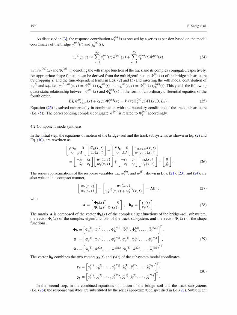
As discussed in [3], the response contribution w(b)r is expressed by a series expansion based on the modal
coordinates of the bridge y(m)b (t) and y(m)
b (t),
w(b)r (x, t) ≈
Nb∑m=1
y(m)b (t)(m)
r (x) +Nb∑m=1
y(m)b (t)(m)
r (x), (24)
with(m)r (x) and
(m)r (x) denoting themth shape function of the track and its complex conjugate, respectively.
An appropriate shape function can be derived from the mth eigenfunction �(m)b (x) of the bridge substructure
by dropping fr and the time-dependent terms in Eqs. (2) and (3) and inserting the mth modal contribution ofw
(b)r and wb, i.e., w
(b)(m)r (x, t) =
(m)r (x)y(m)
b (t) and w(m)b (x, t) = �
(m)b (x)y(m)
b (t). This yields the following
quasi-static relationship between (m)r (x) and �
(m)b (x) in the form of an ordinary differential equation of the
fourth order,E Ir
(m)r,xxxx (x) + kf(x)
(m)r (x) = kf(x)�
(m)b (x)� (x, 0, Lb) . (25)
Equation (25) is solved numerically in combination with the boundary conditions of the track substructure(Eq. (5)). The corresponding complex conjugate
(m)r is related to �
(m)b accordingly.
4.2 Component mode synthesis
In the initial step, the equations of motion of the bridge–soil and the track subsystems, as shown in Eq. (2) andEq. (10), are rewritten as[
ρAb 00 ρAr
] [wb(x, t)wr(x, t)
]+[E Ib 00 E Ir
] [wb,xxxx (x, t)wr,xxxx (x, t)
]
=[−kf kf
kf −kf
] [wb(x, t)wr(x, t)
]+[−cf cf
cf −cf
] [wb(x, t)wr(x, t)
]+[0fr
]. (26)
The series approximations of the response variables wb, w(b)r , and w
(f)r , shown in Eqs. (21), (23), and (24), are
also written in a compact manner,[wb(x, t)wr(x, t)
]=[
wb(x, t)w
(b)r (x, t) + w
(f)r (x, t)
]= �hB, (27)
with
� =[
�b(x)T 0�r(x)T �r(x)T
], hB =
[yb(t)yr(t)
]. (28)
The matrix � is composed of the vector �b(x) of the complex eigenfunctions of the bridge–soil subsystem,the vector �r(x) of the complex eigenfunctions of the track subsystem, and the vector �r(x) of the shapefunctions,
�b =[�
(1)b , �
(2)b , . . . , �
(Nb)b , �
(1)b , �
(2)b , . . . , �
(Nb)b
]T,
�r =[�(1)
r , �(2)r , . . . , �(Nr)
r , �(1)r , �(2)
r , . . . , �(Nr)r
]T,
�r =[(1)
r , (2)r , . . . , (Nb)
r , (1)r , (2)
r , . . . , (Nb)r
]T.
(29)
The vector hB combines the two vectors yb(t) and yr(t) of the subsystem modal coordinates,
yb =[y(1)b , y(2)
b , . . . , y(Nb)b , y(1)
b , y(2)b , . . . , y(Nb)
b
]T,
yr =[y(1)r , y(2)
r , . . . , y(Nr)r , y(1)
r , y(2)r , . . . , y(Nr)
r
]T.
(30)
In the second step, in the combined equations of motion of the bridge–soil and the track subsystems(Eq. (26)) the response variables are substituted by the series approximation specified in Eq. (27). Subsequent
Dynamic analysis of railway bridges 4591
pre-multiplication by �T, and integration over the track length −L0 ≤ x ≤ Lb + L0 leads with the relationbetween the modal accelerations and velocities [20,28],[
ybyr
]=[SbybSryr
](31)
Sb = diag[s(1)b , s(2)
b , . . . , s(Nb)b , s(1)
b , s(2)b , . . . , s(Nb)
b
],
Sr = diag[s(1)r , s(2)
r , . . . , s(Nr)r , s(1)
r , s(2)r , . . . , s(Nr)
r
](32)
finally to the following coupled set of equations track–bridge–soil subsystem in terms of its modal coordinates,
ABhB + BBhB = fB. (33)
The members of the diagonal matrices Sb and Sr: s(m)b , s(m)
b ,m = 1, . . . , Nb; s(n)r , s(n)
r , n = 1, . . . , Nr,are the complex natural frequencies of the bridge–soil and track substructures and their complex conjugatecounterparts, respectively (see Appendices A and B). The system matrices AB and BB,
AB =[Ab + MbSb + Cb MbrSr + CbrMrbSb + Crb Ar
],
BB =[Bb + Kb 00 Br
], (34)
are composed of several sub-matrices, which are explained in the following. The two diagonal sub-matricesAb and Bb contain the coefficients for the orthogonality conditions of the eigenfunctions of the bridge–soilsubsystem a(m)
b , a(m)b , b(m)
b , b(m)b , m = 1, . . . , Nb,
Ab = diag[a(1)b , a(2)
b , . . . , a(Nb)b , a(1)
b , a(2)b , . . . , a(Nb)
b
],
Bb = diag[b(1)b , b(2)
b , . . . , b(Nb)b , b(1)
b , b(2)b , . . . , b(Nb)
b
],
(35)
described in detail in Appendix A. The corresponding matrices for the stand-alone track subsystem, Ar andBr, read as
Ar = diag[a(1)r , a(2)
r , . . . , a(Nr)r , a(1)
r , a(2)r , . . . , a(Nr)
r
],
Br = diag[b(1)r , b(2)
r , . . . , b(Nr)r , b(1)
r , b(2)r , . . . , b(Nr)
r
].
(36)
Details on the coefficients a(n)r , a(n)
r , b(n)r , b(n)
r , n = 1, . . . , Nr, in these matrices are found in Appendix B. Thesub-matrices Mb, Cb, and Kb read as
Mb = ρAr
∫ Lb+L0
−L0
�r�Tr dx,
Cb = − cfb
(∫ Lb
0�b�
Tr dx +
(∫ Lb
0�b�
Tr dx
)T
−∫ Lb
0�b�
Tb dx
)+∫ Lb+L0
−L0
cf�r�Tr dx,
Kb = − kfb
(∫ Lb
0�b�
Tr dx +
(∫ Lb
0�b�
Tr dx
)T
−∫ Lb
0�b�
Tb dx
)+∫ Lb+L0
−L0
kf�r�Tr dx
+E Ir
∫ Lb+L0
−L0
�r�Tr,xxxxdx, (37)
4592 P. König et al.
and the sub-matrices
Mbr = MTrb = ρAr
∫ Lb+L0
−L0
�r�Tr dx,
Cbr = CTrb =
∫ Lb+L0
−L0
cf�r�Tr dx − cfb
∫ Lb
0�b�
Tr dx
(38)
result from coupling of the bridge–soil and the track subsystems.The force vector fB in Eq. (33),
fB =[fbfr
], (39)
captures the effect of the vehicle interaction forces F ( j)k , j = 1, . . . , Nc, k = 1, . . . , 4 (for the considered four
axle vehicles), separately for the bridge–soil subsystem by the vector fb and for the track subsystem by thevector fr. The vector fb reads as
fb =Nc∑j=1
Ψ ( j)r �( j)F( j) , F( j) =
[F ( j)1 , F ( j)
2 , F ( j)3 , F ( j)
4
]T, (40)
where�( j) = diag
[�(t, t ( j)A1 , t ( j)D1 ), �(t, t ( j)A2 , t ( j)D2 ), �
(t, t ( j)A3 , t ( j)D3
), �
(t, t ( j)A4 , t ( j)D4
)](41)
andΨ ( j)
r =[�r
(x ( j)1
), �r
(x ( j)2
), �r
(x ( j)3
), �r
(x ( j)4
)], (42)
with x ( j)i (i = 1, . . . , 4) corresponding to the axle position of each of the four axles of the j th vehicle. The
vector fr is computed according to
fr =Nc∑j=1
Φ( j)r �( j)F( j), (43)
whereΦ( j)
r =[�r
(x ( j)1
), �r
(x ( j)2
), �r
(x ( j)3
), �r
(x ( j)4
)]. (44)
In case of a single load model, where interaction forces in F( j) are assumed to be constant and of knownvalue (i.e., the static axle loads of the train), Eq. (33) can be solved numerically by applying the fourth-orderRunge–Kutta method [6].
5 Coupling of the track–bridge–soil and the train subsystems
First, the equations ofmotion of the track–bridge–soil subsystem, as shown in Eq. (33), and the train subsystem,as shown in Eq. (19), are written in a compact manner,
In Eq. (45), the DOFs at the interface of the two subsystems are still decoupled. The coupling of the axle andthe rail displacements is achieved by the so-called corresponding assumption [45].
According to this assumption, the displacement of each axle of the train corresponds to the underlying raildisplacement including track irregularity, as shown in Figs. 1 and 4. The wheels are thus assumed to be in rigidcontact with the rails, and lift-off is not possible. Approximating the displacement of the track beam wr by amodal series with Nr modes (Eq. (24)), the corresponding assumption yields the vertical displacement of thekth axle (k = 1, . . . , 4)) of the j th vehicle at the position x ( j)
k (t) as follows:
Dynamic analysis of railway bridges 4593
u( j)ak
(x ( j)k
)= wr
(x ( j)k , t
)+ Iirr
(x ( j)k
)
≈Nr∑n=1
�(n)r
(x ( j)k
)y(n)r (t) +
Nr∑n=1
�(n)r
(x ( j)k
)y(n)r (t)
+Nb∑m=1
(m)r
(x ( j)k
)y(m)b (t) +
Nb∑m=1
(m)r
(x ( j)k
)y(m)b (t) + Iirr
(x ( j)k
). (47)
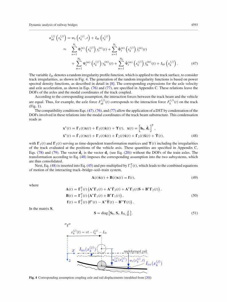
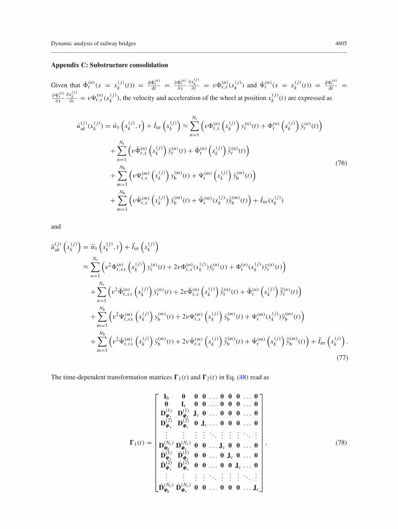
The variable Iirr denotes a random irregularity profile function, which is applied to the track surface, to considertrack irregularities, as shown in Fig. 4. The generation of the random irregularity functions is based on powerspectral density functions, as described in detail in [8]. The corresponding expressions for the axle velocityand axle acceleration, as shown in Eqs. (76) and (77), are specified in Appendix C. These relations leave theDOFs of the axles and the modal coordinates of the track coupled.
According to the corresponding assumption, the interaction forces between the track beam and the vehicleare equal. Thus, for example, the axle force F ( j)
ak (t) corresponds to the interaction force F ( j)k (t) on the track
(Fig. 1).The compatibility conditions Eqs. (47), (76), and (77) allow the application of a DST by condensation of the
DOFs involved in these relations into the modal coordinates of the track beam substructure. This condensationreads as
x∗(t) = �1(t)x(t) + �2(t)x(t) + ϒ(t), x(t) =[hb, dc
with �1(t) and �2(t) serving as time-dependent transformation matrices and ϒ(t) including the irregularitiesof the track evaluated at the positions of the vehicle axis. These quantities are specified in Appendix C,Eqs. (78) and (79). The vector dc is the vector dc (see Eq. (20)) without the DOFs of the train axles. Thetransformation according to Eq. (48) imposes the corresponding assumption into the two subsystems, whichare thus consolidated.
Next, Eq. (48) is inserted into Eq. (45) and pre-multiplied by �T1 (t), which leads to the combined equations
of motion of the interacting track–bridge–soil–train system,
A(t)x(t) + B(t)x(t) = f(t), (49)
whereA(t) = �T
1 (t)(A∗�1(t) + A∗�2(t) + A∗�2(t)S + B∗�2(t)
),
B(t) = �T1 (t)
(A∗�1(t) + B∗�1(t)
),
f(t) = �T1 (t)
(f∗(t) − A∗ϒ(t) − B∗ϒ(t)
).
(50)
In the matrix S,S = diag
[Sb,Sr, INc
ddt
]. (51)
Fig. 4 Corresponding assumption coupling axle and rail displacements (modified from [20])
4594 P. König et al.
Fig. 5 Steps of the model implementation
Table 1 Properties of the soil/foundation and resulting parameters at the bridge boundaries
Properties soil/foundation Parameters bridge-boundariesVariable Value Unit Variable Value Unit
INc denotes the identity matrix of order of the length of dc. Note that only the static axle loads (Eqs. (16)
and (17)) remain in the force vector f(t), and the dynamic interaction forces F ( j)ak (t) and F ( j)
k (t) cancel eachother out when f∗(t) is pre-multiplied by �T
1 (t). The coupled set of equations of motion (Eq. (49)) with time-dependent system matrices is solved by applying the Runge–Kutta method [6]. The steps involved with thesolution procedure of the proposed model are summarized in Fig. 5.
6 Application
6.1 Validation
To validate the proposed semi-analytical modeling approach implemented in MATLAB [25], the results of anapplication example are compared with those of an FE model created in the software suite Abaqus [1]. To thisend, a single-span bridge of length Lb = 21 m, flexural rigidity E Ib = 2.6 · 1010 Nm2, and mass per unitlength ρAb = 7083 kg/m, resting on a moderately stiffness soil with parameters given in Table 1 is considered.
From the soil parameters, by applying Eq. (6) the stiffness and damping coefficients of the spring anddamper below the bridge ends are obtained as kb = 1.276 · 109 N/m2 and cb = 3.229 · 107 Ns/m2. Since thetransient dynamical analysis in Abaqus does not use modal superposition, in the FE model modal damping
Dynamic analysis of railway bridges 4595
Fig. 6 Two-degree-of-freedom MSD system
Table 2 Parameters of two-degree-of-freedom ICE 3 train model [26]
Component Variable Value Unit
1/4 car body mass + 1/2 bogie mass ms 15125 kgAxle mass ma 1800 kgSuspension stiffness ka 1.764 · 106 N/mSuspension damping ca 4.800 · 104 Ns/m
cannot be implemented. Therefore, to ensure comparability of the results, structural damping is not consideredin this example. The parameters of the track subsystem are as follows [3,7]: flexural rigidity E Ir = 8.6 · 106Nm2, mass per unit length ρAr = 103 kg/m, bedding stiffness coefficient kf = 1.316 · 108 N/m2, and beddingdamping coefficient cf = 6.42 · 104 Ns/m2. The length of the track before and after the bridge is chosen asL0 = 30 m, which is much larger than the minimum value according to Eq. (1) (3.21 m). To capture trackirregularities, the random irregularity profile Iirr(x) shown in Fig. 7 is assigned to the rail. This irregularityprofile was created by a stochastic superposition of J harmonic functions as described in [8] with the followinginput parameters: number of harmonic functions J = 1000, characteristic frequencies �c = 0.8246 rad/m,�r = 0.0206 rad/m, �s = 0.4380 rad/m, half distance between rails l = 0.72 m, factor for moderate railquality A = 1.0891 · 10−6, spatial frequency range [π/50, π] rad/m. For details on this procedure and themeaning of the input parameters, it is referred to [8].
In this validation example, the bridge–track system is crossed by the simpleMSD system shown in Fig. 6 atconstant speed v = 80 m/s. That is, instead of a full vehicle with four axles, this MSD system with parametersspecified in Table 2 represents a single axle, half a bogie, and a quarter of a car body of a standard ICE 3train [26]. The corresponding system matrices Ac, Bc, force vector fc, and vector of degrees of freedom uc ofEq. (20) read as
Ac =⎡⎢⎣
ca − ca ms 0−ca ca 0 mams 0 0 00 ma 0 0
⎤⎥⎦ ,
Bc =⎡⎢⎣
ka − ka 0 0−ka ka 0 00 0 ms 00 0 0 ma
⎤⎥⎦ , (52)
fc =⎡⎢⎣
0Fas00
⎤⎥⎦ , uc =
⎡⎢⎣usuausua
⎤⎥⎦ , (53)
with Fas denoting the static axle load.
4596 P. König et al.
Table 3 First six natural complex frequencies of the considered bridge subsystem, the corresponding natural frequencies, andequivalent damping ratios. Natural frequencies of the simply supported bridge subsystem (last column)
Mode m Complex nat. frequ. s(m)b (rad/s) Nat. frequency f (m)
b (Hz) Damping ratio ζ(m)b (%) Nat. frequency (ss) f (m)
When computing the dynamic response using the proposed semi-analytical approach, Nb = 8 modes ofthe stand-alone bridge substructure are taken into account. In Table 3, the first six complex natural frequenciesof these modes and the corresponding natural frequencies ( f (m)
b = Im(s(m)b )/2π = �
(m)b /2π) and equivalent
modal damping ratios due to the dashpot dampers at the beam ends are listed. As can be seen, the second andthird modes are heavily damped with an equivalent damping ratio of close to 80%. In the last column of Table 3also, the first six natural frequencies of the corresponding simply supported bridge (i.e., the subsoil is assumedto be rigid) are listed, showing that the two highly damped modes of the viscoelastically supported structuredo not appear but instead the second natural frequency of the simply supported beam is almost identical withthe fourth of the viscoelastically supported one.
With high values of the bedding coefficient kf , the deflection and acceleration of the rail become veryisolated around a single load leading to a high number of modes required to accurately describe the deformedshape if modal superposition is applied. This fact, albeit mentioned in the literature (e.g., [14]), is oftentimesoverlookedwhenmodal superposition is used in railwaybridgedynamics andwasnot discussed in [3].However,in the presence of track irregularities the modal series of the track substructure must be approximated by asignificantly large number of these modes to correctly predict the bridge response. In the present validationexample, up to Nr = 200 modes of the track subsystem are considered in the response analysis.
In the Abaqus FE model used for validation, the bridge and the track subsystems are discretized by Euler–Bernoulli beam elements of type B23 with an element size of 0.06125 m. To match the rail irregularity profile(Fig. 7) of the semi-analytical model, the element nodes of the rail beam are simply offset from the axis ofthe perfectly straight and smooth track by the amount of the irregularity at the corresponding position x . Theviscoelastic bedding of the track is represented by a series of discrete spring and dashpot elements also spaced0.06125 m apart. The MSD system is modeled as two rigid body lumped masses connected by discrete springand dashpot elements. Since only the vertical motion of the two lumped masses is considered, the rotationalDOFs of the lumped masses are constrained to be zero. The DOF in the horizontal direction is pre-defined bythe speed v = 80 m/s and the initial position at the left support of the rail beam. The vertical DOF of the upperlumped mass is unconstrained, and the contact between axle mass and rail beam is achieved by a so-calledslide line, which models the rigid connection according to the corresponding assumption.
Dynamic analysis of railway bridges 4597
(a) (b)
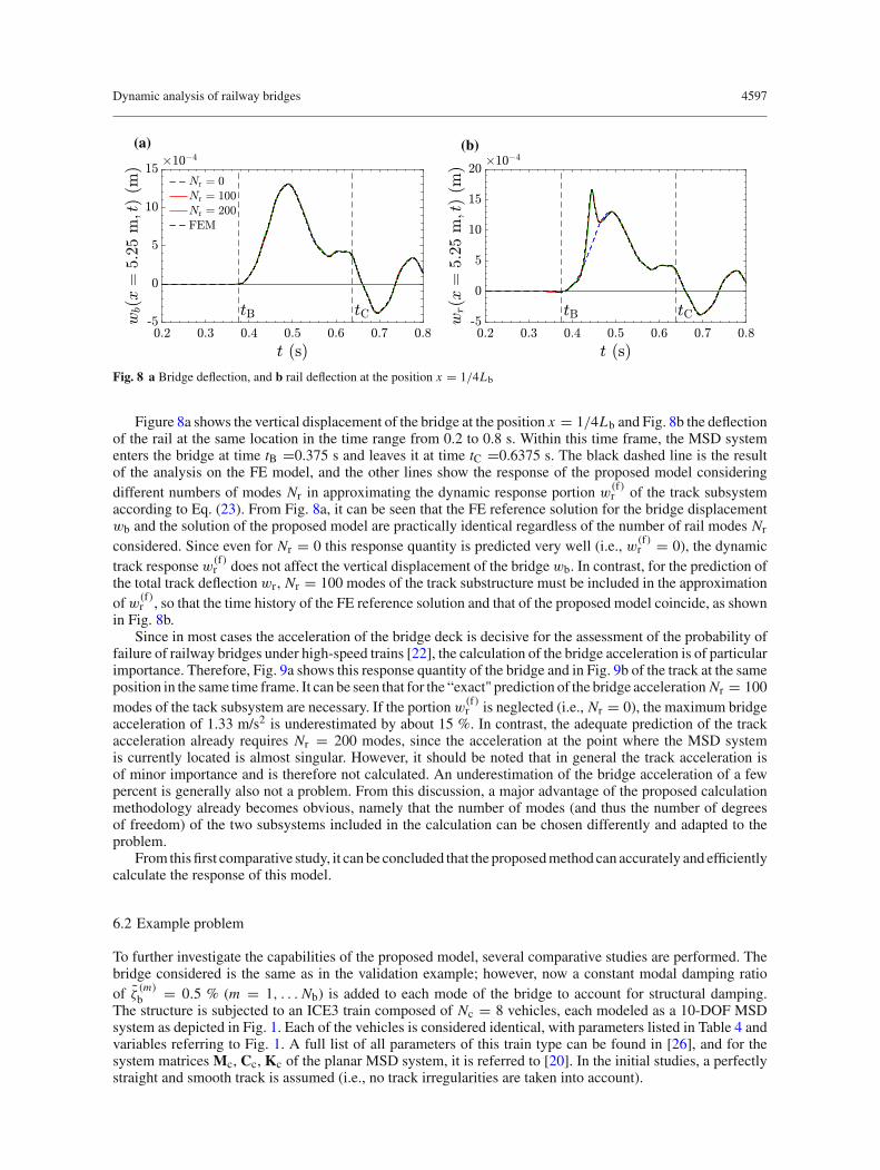
Fig. 8 a Bridge deflection, and b rail deflection at the position x = 1/4Lb
Figure 8a shows the vertical displacement of the bridge at the position x = 1/4Lb and Fig. 8b the deflectionof the rail at the same location in the time range from 0.2 to 0.8 s. Within this time frame, the MSD systementers the bridge at time tB =0.375 s and leaves it at time tC =0.6375 s. The black dashed line is the resultof the analysis on the FE model, and the other lines show the response of the proposed model consideringdifferent numbers of modes Nr in approximating the dynamic response portion w
(f)r of the track subsystem
according to Eq. (23). From Fig. 8a, it can be seen that the FE reference solution for the bridge displacementwb and the solution of the proposed model are practically identical regardless of the number of rail modes Nr
considered. Since even for Nr = 0 this response quantity is predicted very well (i.e., w(f)r = 0), the dynamic
track response w(f)r does not affect the vertical displacement of the bridge wb. In contrast, for the prediction of
the total track deflection wr, Nr = 100 modes of the track substructure must be included in the approximationof w
(f)r , so that the time history of the FE reference solution and that of the proposed model coincide, as shown
in Fig. 8b.Since in most cases the acceleration of the bridge deck is decisive for the assessment of the probability of
failure of railway bridges under high-speed trains [22], the calculation of the bridge acceleration is of particularimportance. Therefore, Fig. 9a shows this response quantity of the bridge and in Fig. 9b of the track at the sameposition in the same time frame. It can be seen that for the “exact" prediction of the bridge acceleration Nr = 100modes of the tack subsystem are necessary. If the portion w
(f)r is neglected (i.e., Nr = 0), the maximum bridge
acceleration of 1.33 m/s2 is underestimated by about 15 %. In contrast, the adequate prediction of the trackacceleration already requires Nr = 200 modes, since the acceleration at the point where the MSD systemis currently located is almost singular. However, it should be noted that in general the track acceleration isof minor importance and is therefore not calculated. An underestimation of the bridge acceleration of a fewpercent is generally also not a problem. From this discussion, a major advantage of the proposed calculationmethodology already becomes obvious, namely that the number of modes (and thus the number of degreesof freedom) of the two subsystems included in the calculation can be chosen differently and adapted to theproblem.
From this first comparative study, it canbe concluded that the proposedmethod can accurately and efficientlycalculate the response of this model.
6.2 Example problem
To further investigate the capabilities of the proposed model, several comparative studies are performed. Thebridge considered is the same as in the validation example; however, now a constant modal damping ratioof ζ
(m)b = 0.5 % (m = 1, . . . Nb) is added to each mode of the bridge to account for structural damping.
The structure is subjected to an ICE3 train composed of Nc = 8 vehicles, each modeled as a 10-DOF MSDsystem as depicted in Fig. 1. Each of the vehicles is considered identical, with parameters listed in Table 4 andvariables referring to Fig. 1. A full list of all parameters of this train type can be found in [26], and for thesystem matrices Mc, Cc, Kc of the planar MSD system, it is referred to [20]. In the initial studies, a perfectlystraight and smooth track is assumed (i.e., no track irregularities are taken into account).
4598 P. König et al.
(a) (b)
Fig. 9 a Bridge acceleration, and b rail acceleration at the position x = 1/4Lb
Table 4 Parameters of the 10-DOF MSD vehicle model [26]
Parameter Variables Value Unit
Mass mp, ms, ma 53500, 3500, 1800 kgMass moment of inertia Ip, Is 1690, 4.569 103kgm2
Dimension hs, ha 17.375, 2.5 mSuspension stiffness ks, ka 820, 17460 kN/mSuspension damping cs, ca 90, 48 kNs/m
As before, the beam response wb is approximated by Nb = 8 series terms and thus also the contributionw
(b)r of the track deflection. In two different approaches, once in the series representation of the dynamic track
deformation w(f)r according to Eq. (23) Nr = 100 modes are considered, and the second time this response
contribution is neglected, w(f)r = 0, i.e., Nr = 0. In a sequence of computations, the speed of the train is
incrementally increased in the range 10 m/s ≤ v ≤ 90 m/s, and the maximum bridge deflection and themaximum bridge acceleration are recorded and plotted against the speed. The resulting representation of thepeak response as a function of v, referred to as response spectra, is shown in Fig. 10. Here, the results onthe left, as shown in Fig. 10a, depict the maximum absolute beam deflection max|wb,rel| = max|(wb(x, t) −(wb(0, t) + x(wb(Lb, t) − wb(0, t))/Lb))|, which corresponds to the vertical displacement without the rigidbody displacement due to the support displacements. The right subfigure, as shown in Fig. 10b, contains themaximum absolute acceleration response of the bridge.
As can be observed, these response spectra exhibit local peaks related to resonance effects resulting fromthe regular axle spacing of the moving MSD system. These peaks are found close to the so-called resonancespeeds, defined as v
(m)j = f (m)
b d/j (j=1,2,3,…), which are directly related to the mth natural frequency ofthe bridge and the characteristic length of the train d [41]. The characteristic length indicates the distance atwhich the moving load pattern of the train repeats and corresponds to the vehicle length d = 24.775 m of theconsidered train. While this definition is exact in the case of a single load model (i.e., the train is representedonly by its static axle loads) in combination with a bridge beam model without track, the observed peak valuesare slightly shifted as a result of the MSD train model due to the additional effects of train mass, damping, andstiffness. In Fig. 10b, some significant resonance speeds are specified, all associated with the first and fourthbridgemodes, keeping inmind that for the viscoelastically supported bridge, the second and thirdmodes (Table3) do not induce resonance effects due to the strongly damped nature of these modes. The most importantfinding of this study is that the deflection of the bridge is virtually unaffected by setting w
(f)r = 0, while the
bridge acceleration is slightly overestimated only in the speed range between 65 and 76 m/s.To illustrate the influence of soil properties on the bridge response, in Fig. 11 the outcomes of the viscoelas-
tically supported structure (referred to as "flexibly supported") are compared with results of the correspondingsimply supported bridge, i.e., the subsoil is assumed to be rigid (referred to as "rigidly supported"), bothbased on Nr = 100 modes for w
(f)r . It can be clearly seen that, in wide speed ranges, both the deflection and
acceleration are much larger for the rigidly supported bridge than for the bridge on a medium-stiff subsoil.This difference is particularly significant at resonance, and, for instance, at the maximum acceleration near
Dynamic analysis of railway bridges 4599
(a) (b)
Fig. 10 a Maximum absolute bridge deflection, and b maximum absolute bridge acceleration for the flexibly supported bridge
(a) (b)
Fig. 11 aMaximum absolute bridge deflection, and bmaximum absolute bridge acceleration for the flexibly and rigidly supportedbridges
the resonance speed v(1)2 it is more than 60%. This result demonstrates how important it can be to include the
properties of the subsoil when calculating the response, albeit often ignored in standard models. In addition,this Figure shows the response spectra of the simply supported bridge for w
(f)r = 0 (i.e., Nr = 0). Here, it can
be seen that for the maximum accelerations in the speed range between 65 and 76 m/s a slight overestimationoccurs compared to the solution considering w
(f)r (Nr = 100).
Subsequently, the influence of the track on the predicted bridge response is investigated, which is alsonot considered in the common beam models. Figure 12 therefore shows, in addition to the results of theproposed model, the solution for the corresponding viscoelastically supported beam without track (referredto as “flexibly supported, no track"). In the latter model, following a recently introduced method [20], theload distribution shortly before and after the bridge is considered in a simplified manner by an approach anda departure phase of lengths La and Ld, respectively. Due to the very isolated deflection of the track aroundthe axle loads, the lengths La = Ld = 1 m were used. For speeds v > 30 m/s, the deflection of the bridgebased on the model without rail and the model presented here agree very well, as shown in Fig. 12a, whilein the lower speed range the model without track subsystem overestimates this response quantity. However,the predicted peak accelerations shown in Fig. 12b depend strongly on the model approach in the entire speedrange. The accelerations predicted with the proposed model are significantly lower than those of the modelwithout rail. This behavior is explained by the improved description of the load distribution over the tracksubsystem as well as possible damping effects due to ballast damping. This result emphasizes the need to takethe track subsystem into account when computing the bridge acceleration, but in many cases, this is usually notdone. As an additional reference, the results of a rigidly supported bridge without track (referred to as “rigidlysupported, no track") are included in Fig. 12, again showing the significantly higher acceleration response ifthe interaction with the underlying soil is neglected.
In this study assuming a perfectly straight and smooth track, no substantial influence of the number ofconsidered rail modes (in w
(f)r ) on the bridge response was observed for the flexibly supported structure.
4600 P. König et al.
(a)(b)
Fig. 12 aMaximum absolute bridge deflection, and bmaximum absolute bridge acceleration for the flexibly and rigidly supportedbridges, with and without the track
(a) (b)
Fig. 13 aMaximum absolute bridge deflection, and bmaximum absolute bridge acceleration, with andwithout track irregularities
To verify this behavior in the presence of track irregularities, the computations are repeated with Nr = 0and Nr = 100 track modes, respectively, however, assigning the random rail irregularity profile Iirr for amoderate quality track shown in Fig. 7 to the track. Figure 13, which compares the bridge response for thesystem with and without track irregularity, shows now a larger effect of these modes on the bridge accelerationwhen irregularities of the track are considered. This effect is more pronounced in the case of the flexiblysupported beam, since the maximum acceleration is underestimated by up to 16.7% when w
(f)r is neglected
(i.e., Nr = 0), compared to the result based on Nr = 100. Further preliminary comparative calculations haveshown that the magnitude of this deviation can be even much larger when other track parameters are used andrail irregularities of a poor quality track are considered. In contrast, the maximum deflection of the bridgeremains largely unaffected by the number of rail modes considered, even in the case of track irregularities,as shown in Fig. 13a. From this study, it can be concluded that the dynamic track deflection w
(f)r has little
effect on bridge displacement, but is more important for accurately predicting the bridge acceleration in thepresence of rail irregularities.
7 Summary and conclusions
In this paper, a novel methodology for predicting the response of railway bridges subjected to high-speedtrains was presented, based on component mode synthesis and a discrete substructuring technique. In the beammodel of the bridge, both the soil under the foundations and the track are included in a simplified manner. Thecoupling of the plane mass–spring–damper model of the train and the non-classically damped soil–bridge–track interaction model is achieved with the so-called corresponding assumption. A major advantage of theproposed methodology is that the number of modes (and thus the number of degrees of freedom) of the tackand the soil–bridge subsystem included in the analysis can be chosen differently and adapted to the problem.A comparative calculation with a less efficient finite element model proved the accuracy of this approach. The
Dynamic analysis of railway bridges 4601
proposed approach allows to investigate effects like soil–structure interaction, bridge–track interaction as wellas bridge–train interaction efficiently and with relatively low numerical effort.
An example bridge was used to show the influence of the subsoil, track, and track irregularities on thenumerically predicted bridge response. From these results, the following preliminary conclusions can bedrawn:
– The results support the well-known fact that dynamic bridge deflection is generally less sensitive to modeldetail than bridge acceleration
– Depending on its properties, the soil can have a significant impact on the predicted bridge response, inparticular at higher speeds and resonance. Due to the radiation damping, over wide speed ranges theresponse of the model with soil is smaller than for the rigidly supported bridge model. At certain trainspeeds, however, an increase of the response can occur due to the frequency reduction and the occurrenceof additional natural frequencies.
– Consideration of the track in the model leads to a reduction in the bridge acceleration due to the load-distributing effect and the damping of the track bed. In contrast, the bridge deflection is hardly influencedby the track model.
– The dynamic response of the track has little effect on the bridge response if the track is perfectly straightand smooth. However, if track irregularities are taken into account, the dynamics of the track can no longerbe neglected when calculating the bridge acceleration, in particular in the higher speed range.
The general validity of these conclusions needs to be substantiated by further extensive parameter studies.
Acknowledgements The computational results presented have been achieved (in part) using the HPC infrastructure LEO of theUniversity of Innsbruck.
Funding Open access funding provided by University of Innsbruck and Medical University of Innsbruck.
Open Access This article is licensed under a Creative Commons Attribution 4.0 International License, which permits use,sharing, adaptation, distribution and reproduction in any medium or format, as long as you give appropriate credit to the originalauthor(s) and the source, provide a link to the Creative Commons licence, and indicate if changes were made. The images or otherthird party material in this article are included in the article’s Creative Commons licence, unless indicated otherwise in a creditline to the material. If material is not included in the article’s Creative Commons licence and your intended use is not permittedby statutory regulation or exceeds the permitted use, you will need to obtain permission directly from the copyright holder. Toview a copy of this licence, visit http://creativecommons.org/licenses/by/4.0/.
Declarations
Competing interests The authors declare that they have no known competing financial interests or personal relationships thatcould have appeared to influence the work reported in this paper.
Funding This research did not receive any specific grant from funding agencies in the public, commercial, or not-for-profitsectors.
Appendix A: Modal properties of the bridge–soil substructure
The eigenfunctions of the Euler–Bernoulli beam bridge substructure [9,43]
�(x) = C1 sinλx
L+ C2 cos
λx
L+ C3 sinh
λx
L+ C4 cosh
λx
L(54)
are adjusted to the boundary conditions (Eq. (12)). Since the beam is non-classically damped due to thespring–damper elements below the bearings, the infinite number of eigenvalues λb resulting from zeroing thecoefficient determinant of the four corresponding equations appears in complex conjugate pairs, referred toas λ
(m)b , (m = 1, . . . ,∞) and its conjugate complex counterpart as λ
(m)b . The mth complex natural frequency
s(m)b of the stand-alone beam, which is related to the mth eigenvalue λ
is composed of a real and an imaginary part, s(m)b = σ
(m)b + i�(m)
b [4,29]. The corresponding conjugate
complex frequency is denoted as s(m)b = σ
(m)b − i�(m)
b . The real part σ (m)b of s(m)
b is referred to as decay rate
and the imaginary part �(m)b as the damped mth natural frequency. The absolute value of s(m)
b is the so-calledpseudo-undamped natural frequency of the bridge beam,
ω(m)b =
∣∣∣s(m)b
∣∣∣ =√(
σ(m)b
)2 +(�
(m)b
)2, (56)
and the ratio
ζ(m)b =
−�(s(m)b
)∣∣∣s(m)b
∣∣∣ = −σ(m)b
ω(m)b
(57)
corresponds to themth modal equivalent damping ratio [19] of the non-classically damped beam substructure.This equivalent damping coefficient takes into account the damping due to the dashpot dampers at the endsof the bridge. If the structural damping of the beam is also to be considered, this is simply done by addingthe mth modal structural damping ζ
(m)b coefficient to the mth modal equivalent damping coefficient ζ (m)
b , i.e.,
ζ(m)b + ζ
(m)b [20]. In this case, the mth complex natural frequency becomes [20]
s(m)b = −ω
(m)b
(ζ
(m)b + ζ
(m)b
)+ iω(m)
b
√1 −
(ζ
(m)b + ζ
(m)b
)2. (58)
By inserting the unmodified eigenvalues λ(m)b into Eq. (54), three of the constants C (m)
1 ,C (m)2 ,C (m)
3 ,C (m)4 of
the mth eigenfunction �(m)b (x) can be expressed by the fourth. This constant can be scaled arbitrarily. The
corresponding conjugate complex eigenfunction is denoted as �(m)b (x).
The orthogonality relations of the eigenfunctions read as [15,20,24]
a(m)b δlm = cb
(�
(m)b (0)�(l)
b (0) + �(m)b (Lb)�
(l)b (Lb)
)+(s(l)b + s(m)
b
)(ρbAb
∫ Lb
0�
(m)b (x)�(l)
b (x)dx
+ mb
(�
(m)b (0)�(l)
b (0) + �(m)b (Lb)�
(l)b (Lb)
)),
(59)
b(m)b δlm = kb
(�
(m)b (0)�(l)
b (0) + �(m)b (Lb)�
(l)b (Lb)
)+ E Ib
∫ Lb
0�
(m)b,xx (x)�
(l)b,xx (x)dx
−(s(m)b s(l)
b
)(ρbAb
∫ Lb
0�
(m)b (x)�(l)
b (x)dx
+ mb
(�
(m)b (0)�(l)
b (0) + �(m)b (Lb)�
(l)b (Lb)
)). (60)
The normalizing constants a(m)b = 2s(m)
b M (m)b and b(m)
b = −2(s(m)b
)2M (m)
b are both related to the generalized
modal mass M (m)b , which can be expressed as
M (m)b = cb
2s(m)b
((�
(m)b (0)
)2 +(�
(m)b (Lb)
)2)
+ ρbAb
∫ Lb
0
(�
(m)b (x)
)2dx + mb
((�
(m)b (0)
)2 +(�
(m)b (Lb)
)2).
(61)
Dynamic analysis of railway bridges 4603
Appendix B: Modal properties of the track substructure
The eigenvalue problem of the track substructure beam model is derived from the homogeneous form of theequation of motion (Eq. (2)),
E Ir�r,xxxx (x) + (s2r ρAr + srcf(x) + kf(x)
)�r(x) = 0, (62)
and the relations yr = sr yr and yr = s2r yr resulting from the general expression yr(t) = Ce(sr t) [20,28].Conveniently, the natural frequencies of this substructure are found considering one half of the track model,because the piecewise differently bedded beam model is symmetric, and thus symmetry and antimetry of theeigenfunctions apply. For the analysis of eigenmodes, half the beam is first divided into the segment abovethe soil and the segment above the bridge. The local axial coordinate of the segment above the soil is denotedas x1 = x + L0 and has its origin at the left end of the track (Fig. 1, point (A)), whereas the axial coordinatefor the section above the bridge denoted as x2 = x has its origin at the left viscoelastic bridge bearing (Fig. 1,point (B)). The eigenvalue problem now written separately for each beam segment,
E Ir�r0,xxxx (x1) + (s2r ρAr + srcf0 + kf0
)�r0(x1) = 0 for 0 ≤ x1 ≤ L0, (63)
E Ir�rb,xxxx (x2) + (s2r ρAr + srcfb + kfb
)�rb(x2) = 0 for 0 < x2 ≤ Lb/2, (64)
yields the eigenmodes in the form of Eq. (54) [9,43],
�r0 (x1) = Cr0(1) sinλr0x1L0
+ Cr0(2) cosλr0x1L0
+ Cr0(3) sinhλr0x1L0
+ Cr0(4) coshλr0x1L0
,
�rb (x1) = Crb(1) sinλrbx2Lb/2
+ Crb(2) cosλrbx2Lb/2
+ Crb(3) sinhλrbx2Lb/2
+ Crb(4) coshλrbx2Lb/2
, (65)
where
λr0 = L04
√− s2r ρAr + srcr0 + kf0
E Ir, λrb = Lb
24
√− s2r ρAr + srcrb + kfb
E Ir. (66)
The eigenvalue λr0 can be expressed in terms of the eigenvalue λrb by solving the equation for λrb in Eq. (66)for the eigenfrequency sr,
sr = 1
2ρAr
(−cfb ±
√c2fb − 4kfbρAr − λ4rbE IrρAr
L40
), (67)
and inserting this relation in the expression for λr0. Adjusting Eq. (65) to the boundary conditions at the leftend of the beam,
�r0 (x1 = 0) = 0, �r0,xx (x1 = 0) = 0, (68)
the continuity conditions between the beam segments,
with Ib being an identity matrix of dimension [2Nb×2Nb] and Ir the identity matrix of dimension [2Nr×2Nr].The matrix
Jc =[I[6×6]c0[4×6]
](80)
indicates the DOFs of the vehicle body and bogies of the j th vehicle by including the identity matrix Ic andsetting the remaining rows, corresponding to the DOFs of the four axles, to zero. The sub-matrices
D( j)Ψ r
(t) =[
0[6×2Nb]
�( j)(t)Ψ ( j)Tr (t)
], D( j)
Φr(t) =
[0[6×2Nr ]
�( j)(t)Φ( j)Tr (t)
](81)
are composed of the shape functions and eigenfunctions of the track evaluated at the axle positions x ( j)k (t)
with �( j)(t) as the previously defined window function only allowing the displacements of axles betweenbeginning and end of the track to be non-zero. The vector
ϒ(t) =[0, I(1)irr (t), I(2)irr (t), . . . , I(Nc)
irr (t)]T
(82)
with
I( j)irr (t) =
⎡⎢⎢⎢⎢⎢⎢⎢⎢⎣
0[6×1]
�(t, t ( j)A1 , t ( j)D1
)Iirr
(x ( j)1 (t)
)�(t, t ( j)A2 , t ( j)D2
)Iirr
(x ( j)2 (t)
)�(t, t ( j)A3 , t ( j)D3
)Iirr
(x ( j)3 (t)
)�(t, t ( j)A4 , t ( j)D4
)Iirr
(x ( j)4 (t)
)
⎤⎥⎥⎥⎥⎥⎥⎥⎥⎦
(83)
is the j th sub-vector containing the irregularity profiles at the four axle positions of the j th vehicle. The vector0 in (82) has 2Nb + 2Nr entries, representing the DOFs of the bridge and track.
References
1. ABAQUS (2016).: Providence, RI, United States (2015)2. Biondi, B., Muscolino, G.: Component-mode synthesis method for coupled continuous and FE discretized substructures.
Eng. Struct. 25(4), 419–433 (2003). https://doi.org/10.1016/S0141-0296(02)00183-93. Biondi, B., Muscolino, G., Sofi, A.: A substructure approach for the dynamic analysis of train-track-bridge system. Comput.
Struct. 83(28–30), 2271–2281 (2005). https://doi.org/10.1016/j.compstruc.2005.03.0364. Brandt, A.: Noise and Vibration Analysis: Signal Analysis and Experimental Procedures/Anders Brandt. Wiley-Blackwell,
Oxford (2011)5. Bucinskas, P., Andersen, L.: Dynamic response of vehicle-bridge-soil system using lumped-parameter models for structure-
soil interaction. Comput. Struct. 238, 106270 (2020). https://doi.org/10.1016/j.compstruc.2020.1062706. Butcher, J.C.: Numerical Methods for Ordinary Differential Equations, 3rd Edn. Wiley, Hoboken, New Jersey (2016)7. Cheng, Y.S., Au, F.T.K., Cheung, Y.K.: Vibration of railway bridges under a moving train by using bridge-track-vehicle
9. Clough, R.W., Penzien, J.: Dynamics of Structures. McGraw-Hill, New York (1993)10. Cojocaru, E.C., Irschik, H., Gattringer, H.: Dynamic response of an elastic bridge due to a moving elastic beam. Comput.
Struct. 82(11), 931–943 (2004). https://doi.org/10.1016/j.compstruc.2004.02.00111. Das, B.M., Luo, Z.: Principles of Soil Dynamics. Cengage Learning (2016)12. Den Hartog, J.P.: Advanced strength of materials. Dover Books on Engineering. Dover Publications, New York (1987)13. Di Lorenzo, S., Di Paola, M., Failla, G., Pirrotta, A.: On the moving load problem in Euler-Bernoulli uniform beams with
viscoelastic supports and joints. Acta Mech. 228(3), 805–821 (2017). https://doi.org/10.1007/s00707-016-1739-614. Dimitrovová, Z.: New semi-analytical solution for a uniformly moving mass on a beam on a two-parameter visco-elastic
foundation. Int. J. Mech. Sci. 127, 142–162 (2017). https://doi.org/10.1016/j.ijmecsci.2016.08.02515. Foss, K.A.: Coordinates which uncouple the equations of motion of damped linear dynamic systems. J. Appl. Mech. 25,
361–364 (1958)16. Frýba, L.: Dynamics of railway bridges. Thomas Telford Publishing (1996). https://doi.org/10.1680/dorb.3471617. Frýba, L.: Vibration of Solids and Structures Under Moving Loads. Springer (1999). https://doi.org/10.1007/978-94-011-
9685-718. Galvín, P., Domínguez, J.: High-speed train-induced ground motion and interaction with structures. J. Sound Vib. 307(3),
755–777 (2007). https://doi.org/10.1016/j.jsv.2007.07.01719. Genta, G.: Vibration Dynamics and Control. Mechanical Engineering Series. Springer, New York (2009)20. Hirzinger, B., Adam, C., Salcher, P.: Dynamic response of a non-classically damped beam with general boundary conditions
subjected to a moving mass-spring-damper system. Int. J. Mech. Sci. 185, 105877 (2020). https://doi.org/10.1016/j.ijmecsci.2020.105877
21. Hirzinger, B., Adam, C., Salcher, P., Oberguggenberger,M.: On the optimal strategy of stochastic-based reliability assessmentof railway bridges for high-speed trains. Meccanica 54(9), 1385–1402 (2019). https://doi.org/10.1007/s11012-019-00999-0
22. Johansson, C., Nualláin, N.Á.N., Pacoste, C., Andersson, A.: A methodology for the preliminary assessment of existingrailway bridges for high-speed traffic. Eng. Struct. 58, 25–35 (2014). https://doi.org/10.1016/j.engstruct.2013.10.011
23. Knothe, K.: Rail Vehicle Dynamics. Springer, Cham, Switzerland (2016)24. Krenk, S.: Complex modes and frequencies in damped structural vibrations. J. Sound Vib. 270(4–5), 981–996 (2004). https://
doi.org/10.1016/S0022-460X(03)00768-525. MATLAB (R2020a). Natick, Massachusetts (2020)26. Nguyen, K., Goicolea, J.M., Galbadón, F.: Comparison of dynamic effects of high-speed traffic load on ballasted track using
a simplified two-dimensional and full three-dimensional model. Proc. Inst. Mech. Eng. Part F: J. Rail Rapid Transit. 228(2),128–142 (2014). https://doi.org/10.1177/0954409712465710
27. Popp, K., Schiehlen, W.O., Kröger, M., Panning, L.: Ground Vehicle Dynamics. Springer, Berlin (2010)28. Pradlwarter, H.: Personal Communication (2018)29. Prater, G., Singh, R.: Eigenproblem formulation, solution and interpretation for non-proportionally damped continuous
beams. J. Sound Vib. 143(1), 125–142 (1990). https://doi.org/10.1016/0022-460X(90)90572-H30. Romero, A., Solís, M., Domínguez, J., Galvín, P.: Soil-structure interaction in resonant railway bridges. Soil Dyn. Earthq.
(2015). https://doi.org/10.1007/s00707-015-1314-632. Stokes, G.G.: Discussion of a Differential Equation Relating to the Breaking of Railway Bridges. Printed at the Pitt Press by
John W. Parker (1849). https://doi.org/10.1017/CBO9780511702259.01333. Stoura, C.D., Dimitrakopoulos, E.G.: A Modified Bridge System method to characterize and decouple vehicle–bridge inter-
action. Acta Mech. 1619–6937 (2020). https://doi.org/10.1007/s00707-020-02699-334. Stoura, C.D., Dimitrakopoulos, E.G.: Additional damping effect on bridges because of vehicle-bridge interaction. J. Sound
Vib. 476, 115294 (2020). https://doi.org/10.1016/j.jsv.2020.11529435. Svedholm, C., Pacoste, C., Karoumi, R.: Modal properties of simply supported railway bridges due to soil-structure interac-
tion. In: M. Papadrakakis, V. Papadopoulos, V. Plervis (eds.) COMPDYN, pp. 1709–1719 (2015)36. Svedholm, C., Zangeneh, A., Pacoste, C., François, S., Karoumi, R.: Vibration of damped uniform beams with general end
conditions under moving loads. Eng. Struct. 126, 40–52 (2016). https://doi.org/10.1016/j.engstruct.2016.07.03737. Ülker-Kaustell, M., Karoumi, R., Pacoste, C.: Simplified analysis of the dynamic soil-structure interaction of a portal frame
railway bridge. Eng. Struct. 32(11), 3692–3698 (2010). https://doi.org/10.1016/j.engstruct.2010.08.01338. Willis, R.: Preliminary essay to the Appendix B: Experiment for determining the effects produced by causing weights to
travel over bars with different velocities. Report of the commissions appointed to inquire into the application of iron torailway structures. W. Clowes and Sons (1849)
39. Wolf, J.P., Deeks, A.: Foundation Vibration Analysis: A Strength of Materials Approach. Butterworth-Heinemann, Oxford(2004)
41. Yang, Y.B., Yau, J.D., Wu, Y.S.: Vehicle–Bridge Interaction Dynamics. With Applications to High-Speed Railways. WorldScientific (2004). https://doi.org/10.1142/5541
42. Zangeneh, A., Svedholm, C., Andersson, A., Pacoste, C., Karoumi, R.: Identification of soil-structure interaction effect in aportal frame railway bridge through full-scale dynamic testing. Eng. Struct. 159, 299–309 (2018). https://doi.org/10.1016/j.engstruct.2018.01.014
43. Zarek, J.H.B., Gibbs, B.M.: The derivation of eigenvalues and mode shapes for the bending motion of a damped beam withgeneral end conditions. J. Sound Vib. 78(2), 185–196 (1981). https://doi.org/10.1016/S0022-460X(81)80032-6
45. Zhang, N., Xia, H., Guo, W.W., De Roeck, G.: A vehicle-bridge linear interaction model and its validation. Int. J. Struct.Stab. Dyn. 10(02), 335–361 (2010). https://doi.org/10.1142/S0219455410003464
46. Zhu, Z., Gong, W., Wang, L., Li, Q., Bai, Y., Yu, Z., Harik, I.E.: An efficient multi-time-step method for train-track-bridgeinteraction. Comput. Struct. 238, 106270 (2017). https://doi.org/10.1016/j.compstruc.2017.11.004
Publisher’s Note Springer Nature remains neutral with regard to jurisdictional claims in published maps and institutionalaffiliations.