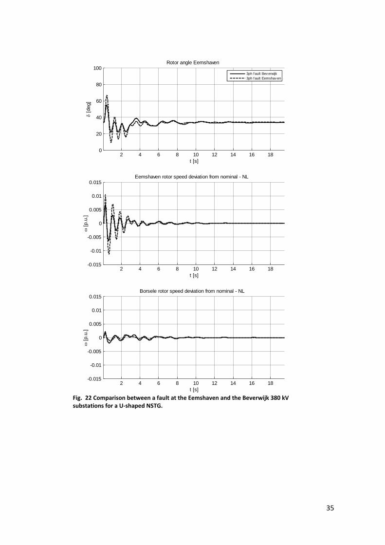
1 Dynamic Behaviour and Transient Stability Assessment of a North‐Sea Region Case Containing VSC‐HVDC Transmission Authors: A. A. van der Meer, M. Ndreko, B. G. Rawn, M. Gibescu WP 6.2. NSTG Project Technical Report, Part II 06/11/2012-08/03/2013 Revised: April 26, 2013 Status: Confidential ESEIEPG Delft University of Technology
Transcript
1
Dynamic Behaviour and Transient Stability Assessment of a North‐Sea Region Case Containing VSC‐HVDC
Transmission Authors: A. A. van der Meer, M. Ndreko, B. G. Rawn, M. Gibescu
WP 6.2. NSTG Project Technical Report, Part II
06/11/2012-08/03/2013
Revised: April 26, 2013
Status: Confidential
ESEIEPG Delft University of Technology
2
Table of Contents Introduction....................................................................................................................................... 3
Introduction Future power systems will contain more renewable energy sources, notably wind and solar in Western Europe. The grid integration challenge grows with the amount of renewables penetration. Offshore wind will have and important share in this challenge, not just from an operational viewpoint, but also from a grid integration respect. High‐voltage DC transmission based on voltage sourced converter technology (VSC‐HVDC) is more and more becoming common practice to interconnect offshore wind, notably in Germany. The North‐Sea transnational grid (NSTG) project deals with design, control, and grid integration of offshore wind power by VSC‐HVDC schemes, with a plain focus on multi‐terminal VSC‐HVDC. Work package (WP) 6 in this research project addresses the grid integration from a planning, operation, and dynamic behaviour respect. The former two comprise WP 6.1, the latter WP 6.2. This report addresses the progress made for the transient stability part of work package 6.2. The goal of this part of the NSTG research project is to investigate the influence future VSC‐HVDC transmission has on dynamics of the interconnected AC system, most notably in the transient stability time‐frame of interest (0.1 — 10 s.) This document is a continuation of the study previously performed on a dynamic model of the Western European system for the North‐Sea Transnational Grid (NSTG) research project [1]. It will test the hypothesis that disturbances between two synchronous areas are propagated when both AC systems are coupled through multi‐terminal VSC‐HVDC. This aspect was shown to be present in the individual synchronous areas already, but the effects on different areas were outside the scope of that research. To draw significantly strong conclusions about this, assumptions have to be made about the characteristics of the future power system. First, the available DC dynamic model had to be improved to a) include an arbitrary number of nodes, branches, and VSC terminals, 2) to allow a correct and numerically stable inclusion into the AC power flow algorithm, and 3) to improve simulation speed by application of hybrid simulation methods developed within this research project [2]. Then, a dynamic equivalent of the British power system was developed based on available literature. This equivalent was adjusted to incorporate the envisaged amount of offshore wind power. The 7.5 GW offshore wind power in Germany that was integrated in the previous work was increased to a total amount of 11 GW. Nuclear power plants were decommissioned to achieve this. The resulting unit commitment reflects a high wind, high‐import scenario for the Netherlands. Using this scenario, several events were studied in the time‐domain, discriminating between point‐to‐point VSC‐HVDC links and a U‐shaped transnational grid that hence interconnects both the Continental European and British systems. All dynamic simulations were executed by using PSSE. This report will continue as follows. First, the modelling assumptions will be discussed, followed by a more detailed case description. Then, the respective event studies will be shown. The report ends with conclusions and recommendations.
4
Modelling Assumptions
General The main focus is the investigation of dynamic phenomena in the transient stability time‐frame of interest, i.e. 0.1 — 10 s. This comprises the dynamic response after faults, with special attention to first‐swing stability. The study presented in this work was performed by PSSE, using a dynamic model of the former UCTE transmission system as a starting point. This dynamic model has been adjusted and extended to more accurately reflect the situation of the foreseen 2020 time‐horizon that was assumed within the NSTG project. VSC‐HVDC is modeled using VSC ratings of 1200 MW, as to align with other work packages of the NSTG project. NSTG landing points with a higher transmission capacity are included as aggregated VSC terminals with a nominal ratings of integer multiples of 1200 MW. Submarine cables have transmission capacities that are a multiple of 2400 MW, caused by the branch limitation of the dc‐grid dynamic model. Offshore wind power plant (WPP) capacities, cable lengths, and VSC landing points were taken from work package 2. Small adjustments were necessary for stable and realistic grid integration (stable from both a numerical and an operational viewpoint.) The focus of the dynamic behaviour investigation is on the main generation locations of the Netherlands foreseen in [3]
VSC and DC grid dynamic model for PSSE Although point‐to‐point VSC‐HVDC connections can be simulated by PSSE by either the HVDC light model (ABB) or the HVDC PLUS (Siemens), the assumptions used in these models do not allow simulation of multi‐terminal VSC‐HVDC schemes. Hence, PSSE contains no standard multi‐terminal VSC‐HVDC dynamic model. Based on models developed during the NSTG project [4], generalized VSC and DC grid models were developed and included as user‐written models into PSSE VSC model A generalized VSC scheme is shown in Fig. 1.It consists of
A. the power electronic VSC interface B. A modulator that converts the controller set points to switching pulses C. Controllers that regulate the converter current by measuring the point of
common coupling (PCC) voltage and setting a modulation signal for the converter voltage, along with a proper implementation of the power electronic current limit. This part also contains a phase‐locked loop that synchronises the VSC control system with the PCC voltage, and hence ensures independent control of active and reactive power.
D. Controllers that provide reference points for the active and reactive currents of the converter.
5
The VSC can either be vector controlled or directly controlled. The former is commonly applied in (strong) ac systems to control active and reactive power, the latter is used in passive systems to provide as voltage to which other equipment can synchonise with. In this case offshore WPPs are connected to VSCs that use direct control.
Fig. 1: General representation of a VSC terminal control scheme
For transient stability simulations, the VSC model shall contain those feature and control systems relevant to the transient stability problem, which results in the following assumptions used in this study.
1. As the network is modelled linearly by complex impedances neglecting time‐derivatives of inductive and capacitive branches, the grid interface should be compatible with this accordingly. The phase reactor is hence modelled by a complex impedance and the modulated voltage is represented by a complex phasor.
2. The coupling between the AC and DC side is achieved by the active power balance between the two rather than the physical coupling by power electronic switching.
3. The influence of the applied modulation scheme is only important when a correct topological representation of the power electronics is included. Hence the modulator is neglected and the control system directly sets the terminal voltage. Alternatively, one could chose to implement the modulator by simple time delays.
4. The current controller is neglected. It has a common rise time around 2—4 ms., which is much faster than the time‐constants in the rest of the network and VSC model. Moreover, the converter grid interface is modelled by complex quantities, which allows instantaneous current changes. As a consequence the cross‐coupling between active and reactive currents can now be solved algebraically rather than by control.
6
5. The PLL is neglected and the VSC control system is assumed to synchronise with the PCC voltage within after every network solution. Alternatively, the PLL can be modelled by simple time‐delay functions.
6. The AC‐side of the converter is represented as a time‐varying Norton equivalent. This saves an algebraic conversion from the current injection set point to the terminal voltage set point. Moreover, PSSE by definition requires all dynamics models to be represented by Norton equivalents.
7. Due to the topological converter interface, the VSC exhibits current source behaviour at the DC side. Therefore, the DC side of the VSC is represented by a time‐varying current source.
A schematic diagram of the implemented VSC model is given in Fig. 2. For VSCs employing direct control, the current injection is given by
where is adjusted by the outer controllers to regulate the terminal voltage.
Fig. 2: VSC model as implemented in PSSE
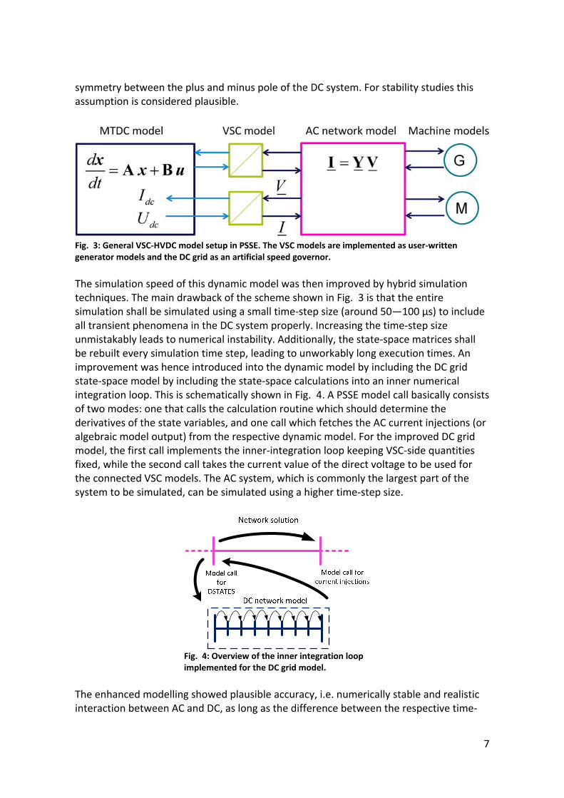
DC grid dynamic model In PSSE, a state‐space representation of the DC grid is applied, which is modelled by an artificial speed governing system supplying multiple VSC generating units. The general model setup is shown in Fig. 3. It can be seen that the DC model uses inputs from multiple VSCs while the VSCs can only access network quantities from the DC grid model and not from neighbouring VSCs. The DC grid is implemented by the state‐space model developed in [5]. It uses a mono‐polar representation of the DC grid, assuming full
7
symmetry between the plus and minus pole of the DC system. For stability studies this assumption is considered plausible.
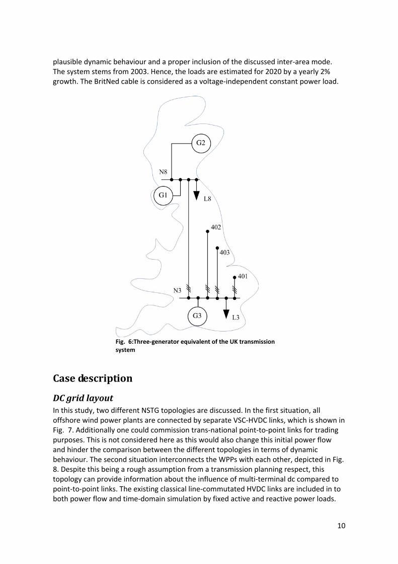
Fig. 3: General VSC‐HVDC model setup in PSSE. The VSC models are implemented as user‐written generator models and the DC grid as an artificial speed governor. The simulation speed of this dynamic model was then improved by hybrid simulation techniques. The main drawback of the scheme shown in Fig. 3 is that the entire simulation shall be simulated using a small time‐step size (around 50—100 µs) to include all transient phenomena in the DC system properly. Increasing the time‐step size unmistakably leads to numerical instability. Additionally, the state‐space matrices shall be rebuilt every simulation time step, leading to unworkably long execution times. An improvement was hence introduced into the dynamic model by including the DC grid state‐space model by including the state‐space calculations into an inner numerical integration loop. This is schematically shown in Fig. 4. A PSSE model call basically consists of two modes: one that calls the calculation routine which should determine the derivatives of the state variables, and one call which fetches the AC current injections (or algebraic model output) from the respective dynamic model. For the improved DC grid model, the first call implements the inner‐integration loop keeping VSC‐side quantities fixed, while the second call takes the current value of the direct voltage to be used for the connected VSC models. The AC system, which is commonly the largest part of the system to be simulated, can be simulated using a higher time‐step size.
Fig. 4: Overview of the inner integration loop implemented for the DC grid model.
The enhanced modelling showed plausible accuracy, i.e. numerically stable and realistic interaction between AC and DC, as long as the difference between the respective time‐
8
step sizes was not too high. Fig. 5 shows a 0.4 s simulation run of a VSC scheme riding through an onshore fault. The dashed line shows the old method whereas the enhanced method is shown by the solid line. The method shown a significant simulation speed improvement, around a factor 7 for small systems and around a factor 15 for the cases simulated in this study. The state‐space model also contains the chopper‐controlled braking resistors to implement fault‐ride through (FRT) behaviour of the scheme. It uses the same control system as in [1]. However, numerical stability showed considerable improvement when the FRT system was modelled by a variable current subtraction rather than by a variable resistor. This especially manifested itself during the multi‐rate implementation of the DC grid model.
0.05 0.1 0.15 0.2 0.25 0.3 0.35 0.40.95
1
1.05
1.1
1.15
direct voltage VSC N 202
V [p
.u.]
t [s]
Δ t = 1 msΔ t = 0.1 ms
Fig. 5 : direct voltage response comparison of a PSSE simulation run with two different time‐step sizes. The solid line shows the DC grid model response using an inner integration loop.
Offshore WPP layout The offshore wind power plant dynamics are only important for the transient stability problem in case the fault‐ride through (FRT) implementation requires controlling the offshore VSC and WPP. As in this case chopper‐controlled braking resistors are used as to achieve FRT. The WPPs are aggregately represented by a type IV wind turbine generator with a WPP equivalent power rating, using the PSSE standard models with default dynamic parameters. The aggregated WTG is connected to the offshore VSC by a zero‐impedance link.
9
Continental system The ac dynamic model basically consists of a relatively detailed (20 kV up to 380 kV) Dutch dynamic model based on the 2010 transmission system layout, and a 380 kV transmission system of Belgium, Germany, and France. Adjacent countries are implemented by dynamic equivalent generators. All generators in the dynamic model have appropriate excitation and speed governing systems. The model is particularly developed for the transient stability time‐frame of interest and does not contain the European inter‐area oscillations properly, which makes is less suitable for small‐signal stability studies.
UK system The previous study [1] did not contain any synchronous area different than the UCTE system. The main extension to the current dynamic model is to add the United Kingdom synchronous area to the dynamic model. This is relevant for several reasons:
1. The NSTG‐project foresees an offshore wind integration amounting to 18 GW on the North‐Sea side of the UK.
2. Integrating this amount of wind power is challenging from an operation, control, and FRT perspective.
3. Interconnecting synchronous areas may connect occurring dynamics to each other. The effect shall be quantified.
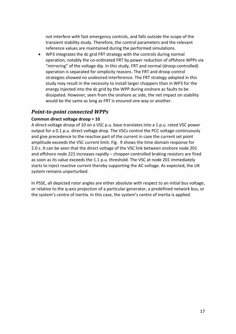
Reproducing the entire UK transmission system may on one hand give the best insight on the effect of the dynamic interaction between the two areas. However, the goal of this work is not to precisely determine the consequences, but rather to 1) quantify when these occur and what the influence of VSC‐HVDC schemes is and to 2) investigate the impact on transient stability on the Continental system. Therefore, a dynamic equivalent was considered appropriate for this research. The 8‐bus, 8‐generator dynamic equivalent proposed and studied in [6] was reproduced and taken as a starting point for integrating the offshore wind proposed in [7]. This model was proven to contain the 0.8 Hz inter‐area mode between Scotland and the English‐Welsh “mainland” system. However, integrating considerable amounts of VSC‐HVDC evacuated wind power introduced very unrealistic power flows and hence voltage distributions, even after implementing necessary transmission expansions. Moreover, the model proofed to be numerically unstable. It could not be retrieved whether this was a particular feature of the reproduced model or the influence of the VSC‐HVDC infrastructure. It was then decided to fall back on the 3‐generator system that formed a basis for the 8‐bus system [8]. This system is shown in Fig. 6. It consists of 2 equivalent generators in Scotland (one in the north and one in the south), which form and inter‐area oscillatory mode with the remainder of the UK system. G3 is the equivalent of this system. The VSC‐HVDC landing points are connected to the high‐voltage terminals of G3 by 380 kV lines having a transmission capacity that equal the WPP capacities. All plants are operated at nominal power employing at a power factor of 0.85 leading. Test disturbances showed
10
plausible dynamic behaviour and a proper inclusion of the discussed inter‐area mode. The system stems from 2003. Hence, the loads are estimated for 2020 by a yearly 2% growth. The BritNed cable is considered as a voltage‐independent constant power load.
Fig. 6:Three‐generator equivalent of the UK transmission system
Case description
DC grid layout In this study, two different NSTG topologies are discussed. In the first situation, all offshore wind power plants are connected by separate VSC‐HVDC links, which is shown in Fig. 7. Additionally one could commission trans‐national point‐to‐point links for trading purposes. This is not considered here as this would also change this initial power flow and hinder the comparison between the different topologies in terms of dynamic behaviour. The second situation interconnects the WPPs with each other, depicted in Fig. 8. Despite this being a rough assumption from a transmission planning respect, this topology can provide information about the influence of multi‐terminal dc compared to point‐to‐point links. The existing classical line‐commutated HVDC links are included in to both power flow and time‐domain simulation by fixed active and reactive power loads.
11
The onshore connection nodes correspond largely to those proposed in work package 2, with the following discrepancies
• The Dogger Bank and the Hornsea wind areas are treated as separate aggregated WPPs.
• One additional German onshore connection (node 102) point was added to foster wind integration in the current ac transmission grid infrastructure.
• Borssele was selected as the main generation location of interest in the duurzame revolutie trend scenario within the Visie2030 study. Hence, this location is added as an NSTG landing point.
A summary of the sub‐marine cable connections is given in Table 1. The amount of wind power connected per offshore node is shown in Table 2; the total amount of integrated wind in this case equals 34 GW.
12
Fig. 7 Point‐to‐point interconnection of offshore wind to be used as reference case
13
UK
B
NL
G
101
102103201
202
203
301
401
403
402
N
422
423
421
321
223
222
221
123
122
121
VSC-HVDCLCC-HVDC
Fig. 8: Implemented North‐Sea Transnational Grid layout. Line lengths are not scaled properly
Table 2 Integrated offshore wind power per WPP node
Unit commitment, wind integration, and transnational power exchange As a starting point, snapshot 3 of [1] was taken. The unit commitment was then adjusted for a higher amount of German wind to be integrated into the power system. This was done by shutting down five nuclear power plants in Germany, amounting to a total generation of 6250 MW that was replaced by offshore wind power. It was then checked
15
to what extent the voltage profile and excitation modes of the remaining generators changed. Subsequently, the generator and VSCs scheduled voltage were altered in such a fashion that most generators were in over‐excitation mode, and hence initiating a more stable starting point for the dynamic simulation. The amount of import to and export from the Netherlands of the resulting power flow is shown in Table 3. Further characteristics of the applied unit commitment scheme are shown in Table 4. It should be emphasised that this particular UC scheme contains very little conventional generation and an unrealistically high utilisation of the wind power plant fleet. Despite being unrealistic, this situation can provide important information about the dynamic behaviour during low‐inertia periods, which will unmistakably occur in the future. The snapshot can also be interpreted as a situation in which a high amount of unwanted import from Germany shall be processed by the Dutch power system.
Belgium Germany United Kingdom
Norway
1474 3750 1000 700 Table 3 Import to (Blue) and export from (red) the Netherlands
Unit commitment
characteristics [MW] Conventional generation
3726
Onshore wind 4234 Offshore wind 5280
Import 3750 Export 3174 Load 13337
Table 4 basic snapshot specifications of the applied UC scheme
16
System Response to a 180 ms threephase busbar fault at the Eemshaven 380 kV substation The first case study comprises a three‐phase short circuit at the busbar of the Eemshaven 380 kV substation. This corresponds to node 201 in Fig. 8. The main reasons for selecting this location are as follows:
1. Eemshaven currently is a key generation location in the Dutch transmission system and its influence will increase in the future. More conventional power plants are presently being commissioned at this location, and new HVDC links to Denmark and Norway are under investigation.
2. Eemshaven is foreseen as a landing point for future offshore wind. In the NSTG project, is it envisaged as a 1200 MW VSC connection point. Faults close to the landing points are more challenging in terms of FRT.
3. Eemshaven is electrically relatively close to the German landing point at the Diele 380 kV substation (node 203 in Fig. 8)
The fault duration is chosen to be 180 ms., which is considered a reasonable clearing time for either distance backup or breaker failure protection. The response of the system for both point‐to‐point VSC‐HVDC transmission and a multi‐terminal U‐shaped offshore grid are of interest. For each topology, we will distinguish between a low direct‐voltage droop setting (10 p.u. on a VSC basis) and a slightly higher one (20 p.u. on a VSC basis). Lower droop settings showed unstable VSC‐HVDC link behaviour whereas higher droop settings resulted in numerical oscillations caused by the applied modelling strategy. In all cases, FRT is accomplished by engaging chopper‐controlled braking resistors when DC voltage rises above 1.1 p.u. For the U‐shaped offshore grid the differences between several control strategies are investigated, namely:
1. All converters control the direct voltage according to a common system direct‐voltage droop line.
2. All UK VSCs are in fixed power control mode, and therefore do not participate in compensating imbalances that might appear in the VSC‐HVDC system as a result of disturbance events.
3. Each country has a single droop‐controlled VSC, which tries to balance voltage fluctuations. The remaining VSCs are in fixed‐power control.
The main similarities and differences compared to the dc grid control methods applied in WP3 are:
• Both approaches apply a droop line in the Pdc—Udc plane to regulate the VSC power output at the ac terminals;
• Both approaches initialise the VSC models taking the corresponding droop line into account inside the dc power flow;
• In practice, the droop lines of the VSCs would be shifted upward or downwards in case the grid operator decides to regulate the dc grid power flows, optimize the voltage profile, or a combination of the two. This process is typically slow so as to
17
not interfere with fast emergency controls, and falls outside the scope of the transient stability study. Therefore, the control parameters and the relevant reference values are maintained during the performed simulations.
• WP3 integrates the dc grid FRT strategy with the controls during normal operation, notably the co‐ordinated FRT by power reduction of offshore WPPs via “mirroring” of the voltage dip. In this study, FRT and normal (droop‐controlled) operation is separated for simplicity reasons. The FRT and droop control strategies showed no undesired interference. The FRT strategy adopted in this study may result in the necessity to install larger choppers than in WP3 for the energy injected into the dc grid by the WPP during onshore ac faults to be dissipated. However, seen from the onshore ac side, the net impact on stability would be the same as long as FRT is ensured one way or another.
Pointtopoint connected WPPs Common direct voltage droop = 10 A direct‐voltage droop of 10 on a VSC p.u. base translates into a 1 p.u. rated VSC power output for a 0.1 p.u. direct voltage drop. The VSCs control the PCC voltage continuously and give precedence to the reactive part of the current in case the current set point amplitude exceeds the VSC current limit. Fig. 9 shows the time domain response for 2.0 s. It can be seen that the direct voltage of the VSC link between onshore node 201 and offshore node 221 increases rapidly – chopper‐controlled braking resistors are fired as soon as its value exceeds the 1.1 p.u. threshold. The VSC at node 201 immediately starts to inject reactive current thereby supporting the AC voltage. As expected, the UK system remains unperturbed. In PSSE, all depicted rotor angles are either absolute with respect to an initial bus voltage, or relative to the q‐axis projection of a particular generator, a predefined network bus, or the system’s centre of inertia. In this case, the system’s centre of inertia is applied.
18
0.5 1 1.5 20
0.5
1
V - EEM380/T6
V [p
.u.]
t [s]0.5 1 1.5 2
0
0.5
1
V - UKN3
V [p
.u.]
t [s]
0.5 1 1.5 20
50
100Rotor angle Eemshaven
δ [d
eg]
t [s]0.5 1 1.5 2
0
50
100Rotor angle UK G3
δ [d
eg]
t [s]
0.5 1 1.5 2-0.02
0
0.02Rotor speed deviation from nominal - NL
ω [p
.u.]
t [s]
Eemshaven
Borsele
0.5 1 1.5 2-0.02
0
0.02Rotor speed deviation from nominal - UK
ω [p
.u.]
t [s]
UKG1
UKG2
UKG3
0.5 1 1.5 20.8
1
1.2
Udc N 201 (NL)
Udc
[p.u
.]
t [s]0.5 1 1.5 2
0.8
1
1.2
Udc N 402 (UK)
Udc
[p.u
.]
t [s]
0.5 1 1.5 2-1
0
1
IDQ VSC N201 (NL)
I [p.
u.]
t [s]
ID
IQ
0.5 1 1.5 2-1
0
1
IDQ VSC N402 (UK)
I [p.
u.]
t [s]
ID
IQ
Fig. 9: System response for a 10 .p.u. dc droop. Left the Continental system, right the UK system.
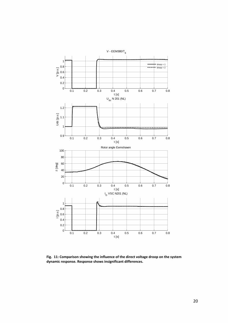
Common‐voltage droop = 20.0 The previous case is now executed with a direct‐voltage droop of 20.0 on the VSC p.u. basis, which allows control of the full VSC output power in a 0.05 p.u. direct voltage range. The response is shown in Fig. 10. It can be seen that also in this case, the system shows stable behaviour.
19
The differences between both cases are plotted in Fig. 11. It can be concluded that that for point‐to‐point VSC connections, hardly any difference in system dynamics can be observed between the two applied droop settings.
0.5 1 1.5 20
0.5
1
V - EEM380/T6
V [p
.u.]
t [s]0.5 1 1.5 2
0
0.5
1
V - UKN3
V [p
.u.]
t [s]
0.5 1 1.5 20
50
100Rotor angle Eemshaven
δ [d
eg]
t [s]0.5 1 1.5 2
0
50
100Rotor angle UK G3
δ [d
eg]
t [s]
0.5 1 1.5 2-0.02
0
0.02Rotor speed deviation from nominal - NL
ω [p
.u.]
t [s]
Eemshaven
Borsele
0.5 1 1.5 2-0.02
0
0.02Rotor speed deviation from nominal - UK
ω [p
.u.]
t [s]
UKG1
UKG2
UKG3
0.5 1 1.5 20.8
1
1.2
Udc N 201 (NL)
Udc
[p.u
.]
t [s]0.5 1 1.5 2
0.8
1
1.2
Udc N 402 (UK)
Udc
[p.u
.]
t [s]
0.5 1 1.5 2-1
0
1
IDQ VSC N201 (NL)
I [p.
u.]
t [s]
ID
IQ
0.5 1 1.5 2-1
0
1
IDQ VSC N402 (UK)
I [p.
u.]
t [s]
ID
IQ
Fig. 10 : System response for a 20 p.u. dc droop. Left the Continental system, right the UK system.
20
0.1 0.2 0.3 0.4 0.5 0.6 0.7 0.80
0.2
0.4
0.6
0.8
1
V - EEM380/T6
V [p
.u.]
t [s]
droop = 1droop = 2
0.1 0.2 0.3 0.4 0.5 0.6 0.7 0.80
20
40
60
80
100Rotor angle Eemshaven
δ [d
eg]
t [s]
0.1 0.2 0.3 0.4 0.5 0.6 0.7 0.80.9
1
1.1
1.2
Udc N 201 (NL)
Udc
[p.u
.]
t [s]
0.1 0.2 0.3 0.4 0.5 0.6 0.7 0.80
0.2
0.4
0.6
0.8
1
ID VSC N201 (NL)
I [p.
u.]
t [s]
Fig. 11: Comparison showing the influence of the direct voltage droop on the system dynamic response. Response shows insignificant differences.
21
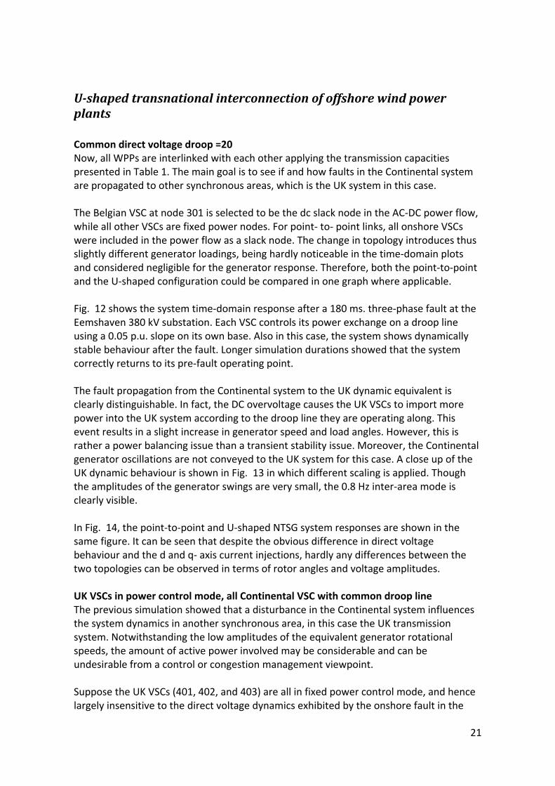
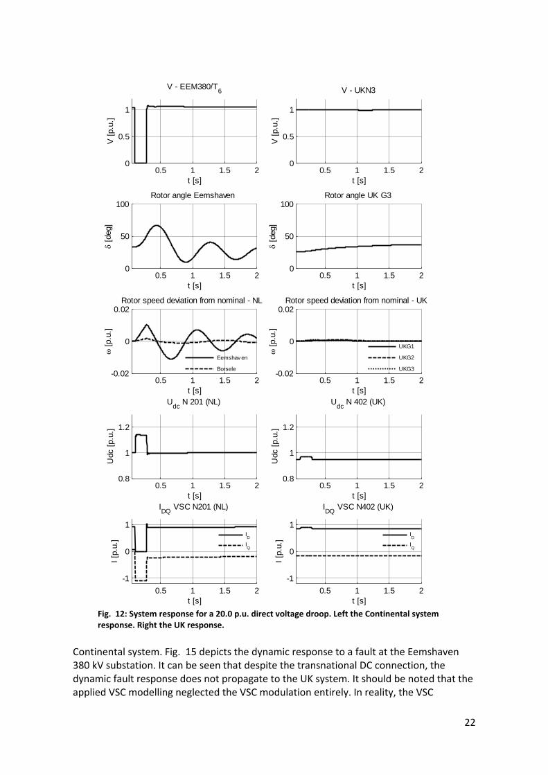
Ushaped transnational interconnection of offshore wind power plants Common direct voltage droop =20 Now, all WPPs are interlinked with each other applying the transmission capacities presented in Table 1. The main goal is to see if and how faults in the Continental system are propagated to other synchronous areas, which is the UK system in this case. The Belgian VSC at node 301 is selected to be the dc slack node in the AC‐DC power flow, while all other VSCs are fixed power nodes. For point‐ to‐ point links, all onshore VSCs were included in the power flow as a slack node. The change in topology introduces thus slightly different generator loadings, being hardly noticeable in the time‐domain plots and considered negligible for the generator response. Therefore, both the point‐to‐point and the U‐shaped configuration could be compared in one graph where applicable. Fig. 12 shows the system time‐domain response after a 180 ms. three‐phase fault at the Eemshaven 380 kV substation. Each VSC controls its power exchange on a droop line using a 0.05 p.u. slope on its own base. Also in this case, the system shows dynamically stable behaviour after the fault. Longer simulation durations showed that the system correctly returns to its pre‐fault operating point. The fault propagation from the Continental system to the UK dynamic equivalent is clearly distinguishable. In fact, the DC overvoltage causes the UK VSCs to import more power into the UK system according to the droop line they are operating along. This event results in a slight increase in generator speed and load angles. However, this is rather a power balancing issue than a transient stability issue. Moreover, the Continental generator oscillations are not conveyed to the UK system for this case. A close up of the UK dynamic behaviour is shown in Fig. 13 in which different scaling is applied. Though the amplitudes of the generator swings are very small, the 0.8 Hz inter‐area mode is clearly visible. In Fig. 14, the point‐to‐point and U‐shaped NTSG system responses are shown in the same figure. It can be seen that despite the obvious difference in direct voltage behaviour and the d and q‐ axis current injections, hardly any differences between the two topologies can be observed in terms of rotor angles and voltage amplitudes. UK VSCs in power control mode, all Continental VSC with common droop line The previous simulation showed that a disturbance in the Continental system influences the system dynamics in another synchronous area, in this case the UK transmission system. Notwithstanding the low amplitudes of the equivalent generator rotational speeds, the amount of active power involved may be considerable and can be undesirable from a control or congestion management viewpoint. Suppose the UK VSCs (401, 402, and 403) are all in fixed power control mode, and hence largely insensitive to the direct voltage dynamics exhibited by the onshore fault in the
22
0.5 1 1.5 20
0.5
1
V - EEM380/T6
V [p
.u.]
t [s]0.5 1 1.5 2
0
0.5
1
V - UKN3
V [p
.u.]
t [s]
0.5 1 1.5 20
50
100Rotor angle Eemshaven
δ [d
eg]
t [s]0.5 1 1.5 2
0
50
100Rotor angle UK G3
δ [d
eg]
t [s]
0.5 1 1.5 2-0.02
0
0.02Rotor speed deviation from nominal - NL
ω [p
.u.]
t [s]
Eemshav en
Borsele
0.5 1 1.5 2-0.02
0
0.02Rotor speed deviation from nominal - UK
ω [p
.u.]
t [s]
UKG1
UKG2
UKG3
0.5 1 1.5 20.8
1
1.2
Udc N 201 (NL)
Udc
[p.u
.]
t [s]0.5 1 1.5 2
0.8
1
1.2
Udc N 402 (UK)
Udc
[p.u
.]
t [s]
0.5 1 1.5 2-1
0
1
IDQ VSC N201 (NL)
I [p.
u.]
t [s]
ID
IQ
0.5 1 1.5 2-1
0
1
IDQ VSC N402 (UK)
I [p.
u.]
t [s]
ID
IQ
Fig. 12: System response for a 20.0 p.u. direct voltage droop. Left the Continental system response. Right the UK response.
Continental system. Fig. 15 depicts the dynamic response to a fault at the Eemshaven 380 kV substation. It can be seen that despite the transnational DC connection, the dynamic fault response does not propagate to the UK system. It should be noted that the applied VSC modelling neglected the VSC modulation entirely. In reality, the VSC
23
modulated voltage by definition depends on the direct voltage level and hence on its transients. The control reaction to this physical coupling is considered much faster than the ac‐system dynamics investigated, and can hence be safely disregarded.
0.5 1 1.5 2 2.5 3 3.5 40
0.2
0.4
0.6
0.8
1
V - UKN3
V [p
.u.]
t [s]
0.5 1 1.5 2 2.5 3 3.5 4-3
-2
-1
0
1
2
3x 10⁻³ Rotor speed deviation from nominal - UK
ω [p
.u.]
t [s]
UKG1
UKG2
UKG3
0.5 1 1.5 2 2.5 3 3.5 4
-1
-0.5
0
0.5
1
IDQ VSC N402 (UK)
I [p.
u.]
t [s]
ID
IQ
Fig. 13: A 4 time‐domain plot of the UK system response, using different scaling.
By (quickly) detecting the faulted synchronous area, the VSCs in the transnationally interlinked areas could be switched to a different control mode such as active power control as part of the FRT control framework. The practical implementation may be difficult because of communication speed, topology dependency, and reliability reasons. However, this is beyond the scope of this research and hence not investigated further.
24
0.05 0.1 0.15 0.2 0.25 0.3 0.35 0.4 0.45 0.50
0.5
1
V - EEM380/T6
V [p
.u.]
t [s]
Point-to-pointU-shaped grid
0.05 0.1 0.15 0.2 0.25 0.3 0.35 0.4 0.45 0.50
50
100Rotor angle Eemshaven
δ [d
eg]
t [s]
0.05 0.1 0.15 0.2 0.25 0.3 0.35 0.4 0.45 0.5-0.02
0
0.02Rotor speed deviation from nominal - NL
ω [p
.u.]
t [s]
0.05 0.1 0.15 0.2 0.25 0.3 0.35 0.4 0.45 0.50.9
1
1.1
1.2
Udc N 201 (NL)
Udc
[p.u
.]
t [s]
0.05 0.1 0.15 0.2 0.25 0.3 0.35 0.4 0.45 0.50
0.5
1
ID VSC N201 (NL)
I [p.
u.]
t [s]
Fig. 14: Comparison between point‐to‐point and multi‐terminal interconnection for a 20.0 p.u. direct voltage droop. The differences are hardly noticeable in the rotor angle response.
25
2 4 6 8 100
0.5
1
V - EEM380/T6
V [p
.u.]
t [s]2 4 6 8 10
0
0.5
1
V - UKN3
V [p
.u.]
t [s]
2 4 6 8 100
50
100Rotor angle Eemshaven
δ [d
eg]
t [s]2 4 6 8 10
0
50
100Rotor angle UK G3
δ [d
eg]
t [s]
2 4 6 8 10-0.02
0
0.02Rotor speed deviation from nominal - NL
ω [p
.u.]
t [s]
Eemshaven
Borsele
2 4 6 8 10-0.02
0
0.02Rotor speed deviation from nominal - UK
ω [p
.u.]
t [s]
UKG1
UKG2
UKG3
2 4 6 8 100.8
1
1.2
Udc N 201 (NL)
Udc
[p.u
.]
t [s]2 4 6 8 10
0.8
1
1.2
Udc N 402 (UK)
Udc
[p.u
.]
t [s]
2 4 6 8 10-1
0
1
IDQ VSC N201 (NL)
I [p.
u.]
t [s]
ID
IQ
2 4 6 8 10-1
0
1
IDQ VSC N402 (UK)
I [p.
u.]
t [s]
ID
IQ
Fig. 15: A 10 s simulation of the NSTG response in case all UK VSCs employ fixed power control. Other VSCs apply a 20.0 p.u. dc droop control Left the Continental system response, right the UK response.
One direct‐voltage controlling node per country Another, more practical situation, might be that all VSCs inside a country or control area dispatch a fixed amount of power except for the one that balances (wind) power
26
variations. This control strategy is applied in Fig. 16, employing the largest VSC of each country as a direct voltage controlling VSC. Again the system shows a stable dynamic response to disturbance applied.
0.5 1 1.5 20
0.5
1
V - EEM380/T6
V [p
.u.]
t [s]0.5 1 1.5 2
0
0.5
1
V - UKN3
V [p
.u.]
t [s]
0.5 1 1.5 20
50
100Rotor angle Eemshaven
δ [d
eg]
t [s]0.5 1 1.5 2
0
50
100Rotor angle UK G3
δ [d
eg]
t [s]
0.5 1 1.5 2-0.02
0
0.02Rotor speed deviation from nominal - NL
ω [p
.u.]
t [s]
Eemshav en
Borsele
0.5 1 1.5 2-0.02
0
0.02Rotor speed deviation from nominal - UK
ω [p
.u.]
t [s]
UKG1
UKG2
UKG3
0.5 1 1.5 20.8
1
1.2
Udc N 201 (NL)
Udc
[p.u
.]
t [s]0.5 1 1.5 2
0.8
1
1.2
Udc N 402 (UK)
Udc
[p.u
.]
t [s]
0.5 1 1.5 2-1
0
1
IDQ VSC N201 (NL)
I [p.
u.]
t [s]
ID
IQ
0.5 1 1.5 2-1
0
1
IDQ VSC N402 (UK)
I [p.
u.]
t [s]
ID
IQ
Fig. 16: Time‐domain response of a situation where each country has 1 DC droop controlled VSC while having the remaining connected VSCs in fixed power control mode.
27
A comparison between the three different control strategies (all droop, UK fixed power, and one dc droop VSC per country) is shown in Fig. 17 for the onshore transmission system quantities, and in Fig. 18 for the UK equivalent generator response respectively.
28
0.05 0.1 0.15 0.2 0.25 0.3 0.35 0.4 0.45 0.50
0.5
1
V - EEM380/T6
V [p
.u.]
t [s]
Solely droop controlUK f ixed P-controlEach country has one droop-controlled VSC
0.05 0.1 0.15 0.2 0.25 0.3 0.35 0.4 0.45 0.50
50
100Rotor angle Eemshaven
δ [d
eg]
t [s]
0.05 0.1 0.15 0.2 0.25 0.3 0.35 0.4 0.45 0.5-0.02
0
0.02Rotor speed deviation from nominal - NL
ω [p
.u.]
t [s]
0.05 0.1 0.15 0.2 0.25 0.3 0.35 0.4 0.45 0.50.9
1
1.1
1.2
Udc N 201 (NL)
Udc
[p.u
.]
t [s]
0.05 0.1 0.15 0.2 0.25 0.3 0.35 0.4 0.45 0.50
0.5
1
ID VSC N201 (NL)
I [p.
u.]
t [s]
Fig. 17: Comparison between the three implemented control strategies. Differences can be observed in the DC voltage and VSC current, but not in the generator responses for the Dutch power system.
29
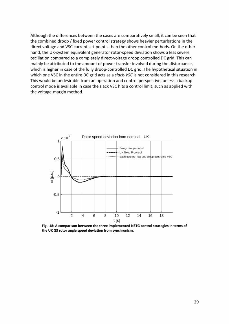
Although the differences between the cases are comparatively small, it can be seen that the combined droop / fixed power control strategy shows heavier perturbations in the direct voltage and VSC current set‐point s than the other control methods. On the other hand, the UK‐system equivalent generator rotor‐speed deviation shows a less severe oscillation compared to a completely direct‐voltage droop controlled DC grid. This can mainly be attributed to the amount of power transfer involved during the disturbance, which is higher in case of the fully droop‐controlled DC grid. The hypothetical situation in which one VSC in the entire DC grid acts as a slack‐VSC is not considered in this research. This would be undesirable from an operation and control perspective, unless a backup control mode is available in case the slack VSC hits a control limit, such as applied with the voltage‐margin method.
2 4 6 8 10 12 14 16 18-1
-0.5
0
0.5
1x 10⁻³ Rotor speed deviation from nominal - UK
ω [p
.u.]
t [s]
Solely droop controlUK f ixed P-controlEach country has one droop-controlled VSC
Fig. 18: A comparison between the three implemented NSTG control strategies in terms of the UK G3 rotor angle speed deviation from synchronism.
30
System Response to a 180 ms threephase busbar fault at the Beverwijk 380 kV substation The second case study entails a busbar fault at the Beverwijk 380 kV substation. This location corresponds to node 202 in Fig. 8. This fault location is chosen for two reasons. First, this location is foreseen to be an important landing point for offshore wind in the future, and hence an onshore connection point within the NSTG research project. Second, the amount of wind power integrated at this location amounts to 3000 MW in the presented study. This is significantly higher than the 1140 MW connected at node 201 of Fig. 8 and it is thus expected that a short‐circuit at node 202 will show more severe power system oscillations. All VSCs in the network are now direct‐voltage droop controlled with the droop constant set at 20.0 p.u. on the VSC base. Similar to the previous case study, the response of the system for both point‐to‐point VSC‐HVDC transmission and a multi‐terminal U‐shaped offshore grid are of interest, after clearing a 180 ms. three‐phase bolted busbar fault.
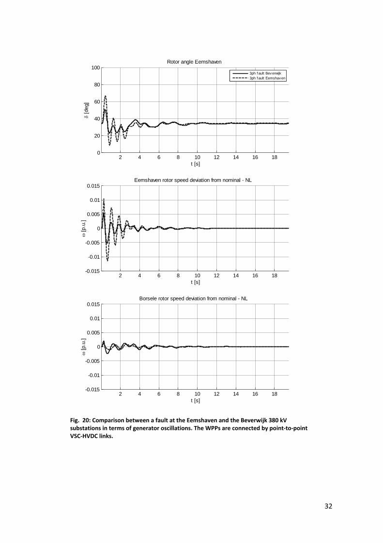
Pointtopoint connection of offshore wind power plants Fig. 19 displays the system response during and after clearing the 180 ms. fault. The system maintains its dynamic stability after fault clearance. It can be plainly observed that the rotor angle of the Eemshaven power plant swings less heavily than with the previous case, particularly due to the electrical distance to the fault. This is also shown in Fig. 20, which compares the Eemshaven and Borssele generator responses for the two fault locations. The chopper‐controlled braking resistor keeps the direct voltage inside the sub‐marine cable connection 222‐202 at a value of 1.2 p.u. while the FRT control system is triggered at a threshold value of 1.1 p.u. This is different from the response of the 221 ‐ 201 DC link discussed in the previous case study. The difference occurs due to the fact that the capacitance in the dc link is now higher since the 222‐202 link is rated at 4800 MW, double the rating of the 221‐201 link
31
0.5 1 1.5 20
0.5
1
V - VSC202
V [p
.u.]
t [s]0.5 1 1.5 2
0
0.5
1
V - UKN3
V [p
.u.]
t [s]
0.5 1 1.5 20
50
100Rotor angle Eemshaven
δ [d
eg]
t [s]0.5 1 1.5 2
0
50
100Rotor angle UK G3
δ [d
eg]
t [s]
0.5 1 1.5 2-0.02
-0.01
0
0.01
0.02Rotor speed deviation from nominal - NL
ω [p
.u.]
t [s]
Eemshav en
Borsele
0.5 1 1.5 2-0.02
-0.01
0
0.01
0.02Rotor speed deviation from nominal - UK
ω [p
.u.]
t [s]
UKG1
UKG2
UKG3
0.5 1 1.5 20.80.9
11.11.2
Udc N 202 (NL)
Udc
[p.u
.]
t [s]0.5 1 1.5 2
0.80.9
11.11.2
Udc N 402 (UK)
Udc
[p.u
.]
t [s]
0.5 1 1.5 2-1
-0.5
0
0.51
IDQ VSC N202 (NL)
I [p.
u.]
t [s]
ID
IQ
0.5 1 1.5 2-1
-0.5
0
0.51
IDQ VSC N402 (UK)
I [p.
u.]
t [s]
ID
IQ
Fig. 19: Dynamic response after a fault at the Beverwijk substation. Left the Continental system, right the UK system response.
32
2 4 6 8 10 12 14 16 180
20
40
60
80
100Rotor angle Eemshaven
δ [d
eg]
t [s]
3ph f ault Bev erwijk3ph f ault Eemshaven
2 4 6 8 10 12 14 16 18-0.015
-0.01
-0.005
0
0.005
0.01
0.015Eemshaven rotor speed deviation from nominal - NL
ω [p
.u.]
t [s]
2 4 6 8 10 12 14 16 18-0.015
-0.01
-0.005
0
0.005
0.01
0.015Borsele rotor speed deviation from nominal - NL
ω [p
.u.]
t [s] Fig. 20: Comparison between a fault at the Eemshaven and the Beverwijk 380 kV substations in terms of generator oscillations. The WPPs are connected by point‐to‐point VSC‐HVDC links.
33
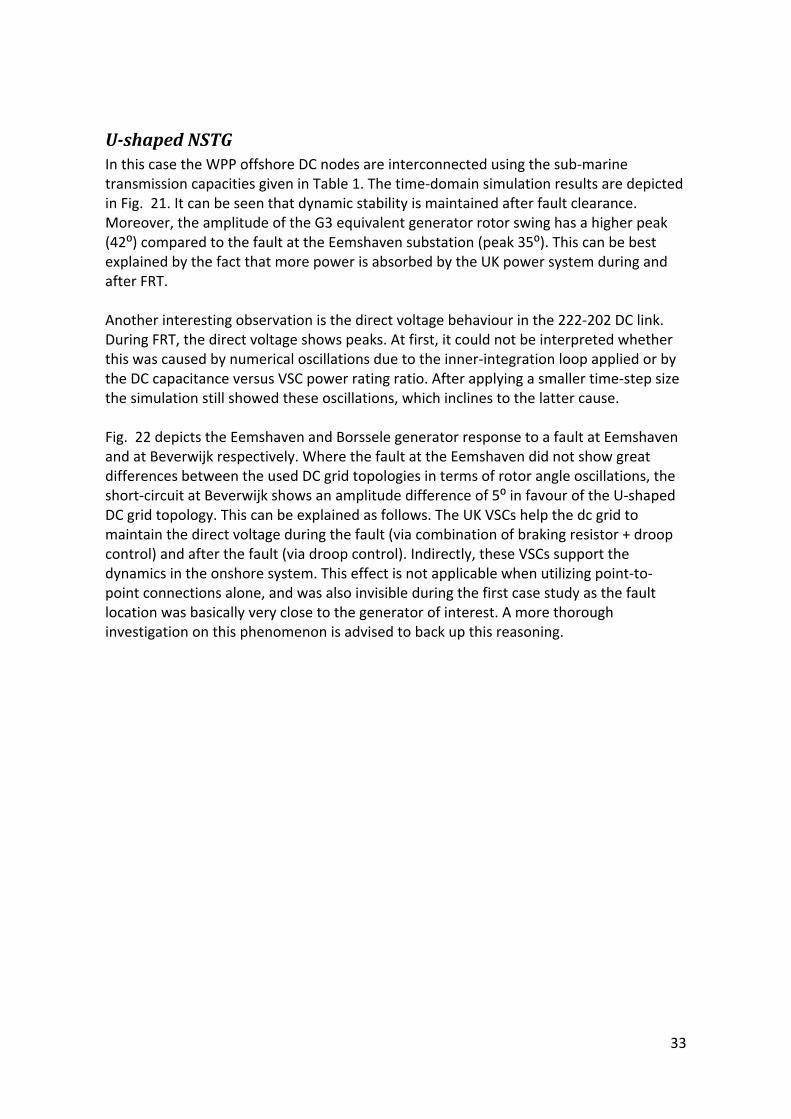
Ushaped NSTG In this case the WPP offshore DC nodes are interconnected using the sub‐marine transmission capacities given in Table 1. The time‐domain simulation results are depicted in Fig. 21. It can be seen that dynamic stability is maintained after fault clearance. Moreover, the amplitude of the G3 equivalent generator rotor swing has a higher peak (42⁰) compared to the fault at the Eemshaven substation (peak 35⁰). This can be best explained by the fact that more power is absorbed by the UK power system during and after FRT. Another interesting observation is the direct voltage behaviour in the 222‐202 DC link. During FRT, the direct voltage shows peaks. At first, it could not be interpreted whether this was caused by numerical oscillations due to the inner‐integration loop applied or by the DC capacitance versus VSC power rating ratio. After applying a smaller time‐step size the simulation still showed these oscillations, which inclines to the latter cause. Fig. 22 depicts the Eemshaven and Borssele generator response to a fault at Eemshaven and at Beverwijk respectively. Where the fault at the Eemshaven did not show great differences between the used DC grid topologies in terms of rotor angle oscillations, the short‐circuit at Beverwijk shows an amplitude difference of 5⁰ in favour of the U‐shaped DC grid topology. This can be explained as follows. The UK VSCs help the dc grid to maintain the direct voltage during the fault (via combination of braking resistor + droop control) and after the fault (via droop control). Indirectly, these VSCs support the dynamics in the onshore system. This effect is not applicable when utilizing point‐to‐point connections alone, and was also invisible during the first case study as the fault location was basically very close to the generator of interest. A more thorough investigation on this phenomenon is advised to back up this reasoning.
34
0.5 1 1.5 20
0.5
1
V - VSC202
V [p
.u.]
t [s]0.5 1 1.5 2
0
0.5
1
V - UKN3
V [p
.u.]
t [s]
0.5 1 1.5 20
50
100Rotor angle Eemshaven
δ [d
eg]
t [s]0.5 1 1.5 2
0
50
100Rotor angle UK G3
δ [d
eg]
t [s]
0.5 1 1.5 2-0.02
0
0.02Rotor speed deviation from nominal - NL
ω [p
.u.]
t [s]
Eemshaven
Borsele
0.5 1 1.5 2-0.02
0
0.02Rotor speed deviation from nominal - UK
ω [p
.u.]
t [s]
UKG1
UKG2
UKG3
0.5 1 1.5 20.8
1
1.2
Udc N 201 (NL)
Udc
[p.u
.]
t [s]0.5 1 1.5 2
0.8
1
1.2
Udc N 402 (UK)
Udc
[p.u
.]
t [s]
0.5 1 1.5 2-1
0
1
IDQ VSC N202 (NL)
I [p.
u.]
t [s]
ID
IQ
0.5 1 1.5 2-1
0
1
IDQ VSC N402 (UK)
I [p.
u.]
t [s]
ID
IQ
Fig. 21: Time‐domain response of for a fault at the Beverwijk 380 kV substation. All VSCs apply droop control. Left the Continental system, right the UK system response.
35
2 4 6 8 10 12 14 16 180
20
40
60
80
100Rotor angle Eemshaven
δ [d
eg]
t [s]
3ph f ault Bev erwijk3ph f ault Eemshaven
2 4 6 8 10 12 14 16 18-0.015
-0.01
-0.005
0
0.005
0.01
0.015Eemshaven rotor speed deviation from nominal - NL
ω [p
.u.]
t [s]
2 4 6 8 10 12 14 16 18-0.015
-0.01
-0.005
0
0.005
0.01
0.015Borsele rotor speed deviation from nominal - NL
ω [p
.u.]
t [s] Fig. 22 Comparison between a fault at the Eemshaven and the Beverwijk 380 kV substations for a U‐shaped NSTG.
36
System response to a sudden loss of an aggregated 3000 MW WPP In the previous sections, short‐circuit faults were the most prominent phenomena of interest, mainly because of the transient stability focus of this work. Now, a sudden loss of a 3000 MW aggregated offshore WPP will be studied. This is close to the maximum allowed loss of generation inside the European synchronous area. Again, distinction is being made between point‐to‐point VSC‐HVDC links only and transnational grid.
Pointtopoint connection of offshore wind power plants The first case, shown in Fig. 23, is a 30 s. simulation run after tripping of the WPP connected at node 121. This immediately causes the VSC at node 101 to cease delivering any active power to the system. In fact, this VSC just balances the direct voltage, the VSC connected at node 102stops drawing active power from the aggregated WPP. This sudden loss manifests itself by the governor reaction of the generation fleet (here, only the Eemshaven power plant is shown). The system establishes itself into a new operating point, indicating that the frequency response of the system is properly included into the power system dynamic model, in particular after the implemented grid reinforcements and the adjusted unit commitment. As can be seen, this transition is relatively slow and hence outside the transient stability time‐frame of interest. It can also be seen that the voltage amplitudes are not affected by this event, which plainly follows from the general conception that excitation systems control the voltage while governing systems maintain the active power balance. As mentioned before, all depicted rotor angles are relative to the system’s centre of inertia. PSSE does not allow direct output of the internal rotor angle nor setting multiple references in case of multi‐area systems. The former software limitation has as a consequence that the shown rotor angle is not directly related to the power output of the generator. The course of the rotor angle after a disturbance now basically depends on three phenomena.
• the power output change in of the generator of interest; • the power output change of the slack generator; and • power flow alternations in the connected network.
The consequence of not allowing multiple references are ostensible angle drifts in asynchronous areas in case rotor speeds differ from the reference synchronous area. This will be shown in the next case study. Due to the chosen reference system, the rotor angle decrement of the Eemshaven power plant may appear unconventional and conflicts with the general perception that the rotor angle is associated with active power output. However, careful consideration of the generator diagram of the Eemshaven power plant showed plausible active and reactive power outputs as well as correct limiting behaviour by the turbine governors. After the
37
oscillatory period the generator re‐established around the pre‐fault operating point. The reduced rotor angle can hence fully be attributed to the slack generator that increases its active power output as well as the power flow that redistributes after the disconnection of the offshore WPP. Being basically constituted by the d—q current projection, the active and reactive power response of the VSC connected to node 201 support this hypothesis.
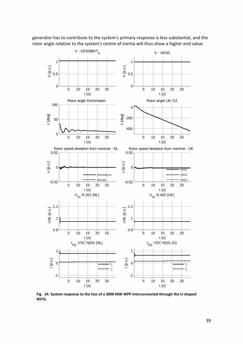
Ushaped transnational offshore interconnection of offshore wind power plants The same situation is now being performed having a trans‐national U‐shaped DC grid to evacuate the offshore wind power. From a power‐system operation viewpoint this is a more interesting case as the other synchronous areas do now have to share in the frequency response after the loss of generation situated outside the area. Fig. 24 shows a 30 s. time‐domain plot of the system reaction after losing the particular offshore WPP. It can be seen that the direct voltage establishes at approximately 0.95 p.u., which is acceptable yet at the boundary of what is still adequate from an operational point of view. Plainly observable is the reaction of the UK equivalent system. At first sight, the generator angles seem to drift away indicating unstable conditions. However, the UK system is not synchronously connected to the onshore transmission system. While the reference angle is the system’s centre of inertia, the frequency in the UK system establishes at a different level compared to the Continental system. The rotor angles of the UK generators result from the integrated frequency difference with the Continental system and the exhibited behaviour thus shows proper island operation. Proper VSC‐HVDC controls could avert or enhance this behaviour, taking trans‐national agreements into account.
38
5 10 15 20 250
0.5
1
V - EEM380/T6
V [p
.u.]
t [s]5 10 15 20 25
0
0.5
1
V - UKN3
V [p
.u.]
t [s]
5 10 15 20 250
50
100Rotor angle Eemshaven
δ [d
eg]
t [s]5 10 15 20 25
0
50
100Rotor angle UK G3
δ [d
eg]
t [s]
5 10 15 20 25-0.02
0
0.02Rotor speed deviation from nominal - NL
ω [p
.u.]
t [s]
Eemshav en
Borsele
5 10 15 20 25-0.02
0
0.02Rotor speed deviation from nominal - UK
ω [p
.u.]
t [s]
UKG1
UKG2
UKG3
5 10 15 20 250.8
1
1.2
Udc N 201 (NL)
Udc
[p.u
.]
t [s]5 10 15 20 25
0.8
1
1.2
Udc N 402 (UK)
Udc
[p.u
.]
t [s]
5 10 15 20 25-1
0
1
IDQ VSC N201 (NL)
I [p.
u.]
t [s]
ID
IQ
5 10 15 20 25-1
0
1
IDQ VSC N101 (G)
I [p.
u.]
t [s]
ID
IQ
Fig. 23: system reaction to a sudden loss of the 3000 MW offshore WPP connected at node 102 (point –to‐point VSC connections).
The reaction of two Dutch generators after losing the WPP at node 102 is depicted on top of each other in Fig. 25 for both DC grid topologies. The main difference is observable in the Eemshaven generator rotor angle response. Applying the direct‐voltage droop power dispatching strategy, the trans‐national grid ensures that loss of generation connected to the DC grid is being resolved by all connected synchronous areas. Compared to the point‐to‐point based connection scheme, therefore, the share each Continental system
39
generator has to contribute to the system’s primary response is less substantial, and the rotor angle relative to the system’s centre of inertia will thus show a higher end value.
5 10 15 20 250
0.5
1
V - EEM380/T6V
[p.u
.]
t [s]5 10 15 20 25
0
0.5
1
V - UKN3
V [p
.u.]
t [s]
5 10 15 20 250
50
100Rotor angle Eemshaven
δ [d
eg]
t [s]5 10 15 20 25
-400
-200
0
Rotor angle UK G3
δ [d
eg]
t [s]
5 10 15 20 25-0.02
0
0.02Rotor speed deviation from nominal - NL
ω [p
.u.]
t [s]
Eemshaven
Borsele
5 10 15 20 25-0.02
0
0.02Rotor speed deviation from nominal - UK
ω [p
.u.]
t [s]
UKG1
UKG2
UKG3
5 10 15 20 250.8
1
1.2
Udc N 201 (NL)
Udc
[p.u
.]
t [s]5 10 15 20 25
0.8
1
1.2
Udc N 402 (UK)
Udc
[p.u
.]
t [s]
5 10 15 20 25-1
0
1
IDQ VSC N201 (NL)
I [p.
u.]
t [s]
ID
IQ
5 10 15 20 25-1
0
1
IDQ VSC N101 (G)
I [p.
u.]
t [s]
ID
IQ
Fig. 24. System response to the loss of a 3000 MW WPP interconnected through the U‐shaped NSTG.
40
2 4 6 8 10 12 14 16 18 200
20
40
60
80
100Rotor angle Eemshaven
δ [d
eg]
t [s]
point-to-point links onlyU-shaped NSTG
2 4 6 8 10 12 14 16 18 20-0.015
-0.01
-0.005
0
0.005
0.01
0.015Eemshaven rotor speed deviation from nominal - NL
ω [p
.u.]
t [s]
2 4 6 8 10 12 14 16 18 20-0.015
-0.01
-0.005
0
0.005
0.01
0.015Borsele rotor speed deviation from nominal - NL
ω [p
.u.]
t [s]
Fig. 25: Comparison between point‐to‐point and the U‐shaped interconnection after losing a 3000 MW WPP.
41
CCT Assessment for Principal Generation Locations Critical clearing times (CCT) are associated with the (in)ability of the synchronous generators in a particular system to maintain the magnetic coupling between the stator and rotor field after events, most importantly short circuits. Corresponding rotors will accelerate during the fault and decelerate after fault clearance. If the clearing time was short enough, the rotor magnetic field magnetic keeps coupled with the rotating stator field and corresponding oscillations superposed to the nominal rotation speed are damped out by the rotor and stator electric and magnetic circuits accordingly. If during this deceleration after fault clearance the magnetic pole of rotor circuit slips away from the rotating stator field it is coupled to, the rotor either slips to the next magnetic pole or drifts away. In elementary systems this behaviour can best be quantified by the equal‐area criterion in the δ‐P plane, and CCTs can even be calculated analytically under some assumptions [9]. The multi‐machine system considered in this study is more complex, not in the least owing to the non‐linear load models and VSC close to the considered generator locations. Hence, CCTs have been calculated by considering the time‐domain simulation results for several fault durations. Table 5 show the CCTs for three‐phase short circuits at the terminals 20 kV terminals of the Eemshaven and Borssele generators. The CCTs have been calculated with an accuracy of 5 ms. Higher accuracy would be unrealistic as the fault is cleared per phase in practice whereas the used dynamic model does not allow inclusion of this asymmetry. Slight differences between the U‐shaped NSTG and point‐to‐point links can be observed, in favour of the latter. This could be explained by the propagation of faults through the dc system, but no strict conclusions can be associated with this. Switching the VSCs from continuous voltage control to fixed reactive power control did not sort any noticeable effect. Therefore, a sensitivity analysis on the generator loading, unit commitment as well as the fault location is advised.
Eemshaven Borssele
U‐shaped 340 295 Point‐to‐point 345 310
Table 5: Critical clearing times for the investigated dc grid topologies and selected generators.
42
Conclusions This study focussed on the implementation of ( a U‐shaped ) North Sea transnational grid structure as was proposed in WP2 into the existing UK and continental European grid models, notably the adjusted dynamic model that is at the disposal of TU Delft from TenneT TSO B.V. under non‐disclosure agreements. The calculation method of the dc grid dynamics within the PSSE tool was explained, as well as the main modelling assumptions and implemented grid expansions. A total amount of 35 GW offshore wind power was integrated, with the Netherlands accounting for 6 GW. Onshore wind power was modelled for the Netherlands only, with a wind generation fleet amounting to a total of 6 GW. Then several cases studies on the interconnected network model were performed, with the following goals:
1. Show the system time‐domain response after test disturbances 2. Show the differences between several offshore grid topologies in terms of power
system dynamics 3. Assess critical clearing times for a couple of generators and quantify the influence
of the NSTG topology It was shown that short circuits in one synchronous area are propagated not only to other VSC landing points in the same synchronous area, but also to asynchronous areas, in this case from the Continental system to the UK. Changing the applied power dispatching technique may improve or compound system dynamics in these cases. It was also shown that rotor oscillations are less prominent when operating the DC grid transnationally. However, more investigation is necessary to make this conclusion stronger. The CCTs for two generation locations have been calculated, both for a U‐shaped NSTG and point‐to‐point links. The differences observed are very small and lie too close to each other to draw any significant conclusions.
Recommendations The applied dc grid control strategy influences system dynamics after the fault. This effect has been quantified but not intensively studied. The main question is whether it is from a control perspective possible to completely isolate the dynamics of the considered asynchronous areas from each other, in most practical situations. Yet, further research efforts could be made either in the NSTG project or in follow‐up research projects to back the conclusions drawn on this. The same applies to the conducted CCT analysis. To achieve this, the grid expansions described below are recommended Several foreseen power plants and reinforcements in the transmission system of the Netherlands have to be added to make the grid model more realistic. The German system is of significant influence on the characteristics of the entire system dynamics. In that respect, the planned HVDC corridors to evacuate the offshore wind from North Germany to the inland load areas (locations) shall be incorporated as realistic
43
as possible. The recent decision to decommission nuclear power plants is only partly implemented in the presented study. Future work should encompass a realistically updated generation fleet. The current dynamic model does not comprise the Western Danish transmission system, which shall be included by a simple but realistic equivalent because 1) the Danish system contains landing points for the North‐Sea transnational grid proposed in WP2 and 2) the Danish system might influence the power system dynamics after the first‐swing time‐frame (500 ms. – 10 s.). A Nordel system dynamic model is at the disposal of the TU Delft but is still to be included in the dynamic models used in this study. The effects on the dynamic behaviour and transient stability are expected to be very small compared to adding the UK system, because the transnational power flows are (potentially) lower compared to power exchange between the UK and the Continental system. Above grid expansions allow reproduction of phase 10 proposed in WP 2. This could strengthen the conclusions related to meshed versus radial DC structures. The current study investigates only one unit commitment case. From a dynamic behaviour respect, interesting situations are considered to be:
1. One or more Dutch VSCs are exporting rather than importing wind power; and 2. A high‐wind, high‐export case which contains considerable ac line flows.
These situations are hence advised as a follow‐up study.
44
References [1] M. Ndreko, “Offshore wind power connected to the Dutch transmission system by VSC‐HVDC networks: Modeling and stability analysis,” Master’s thesis, Delft University of Technology, 2012. [2] A. A. van der Meer, R. L. Hendriks, M. Gibescu, J. A. Ferreira, M. A. M. M. van der Meijden, and W. L. Kling, “Combined simulation method for improved performance in grid integration studies including multi‐terminal VSC‐HVDC,” in Proc. Renewable Power Generation conference, Edinburgh, United Kingdom, Sep. 6–8, 2011. [3] “Visie2030,” TenneT, Tech. Rep., 2010. [4] A. A. van der Meer, R. L. Hendriks, and W. L. Kling, “Combined stability and electro‐magnetic transients simulation od offshore wind power connected through multi‐terminal VSC‐HVDC,” in Proc. PES General Meeting, 2010, (C) AAvdM. [5] P. J. D. Chainho, A. A. van der Meer, R. L. Hendriks, M. Gibescu, and M. A. M. M. van der Meijden, “General modeling of multi‐terminal VSC‐HVDC systems for transient stability studies,” in 6th IEEE Young Researchers Symposium in Electrical Power Engineering, Delft, the Netherlands, Apr. 16–17 2012. [6] T. Knuppel, J. N. Nielsen, K. Jensen, A. Dixon, and J. Ostergaard, “Small‐signal stability of wind power system with full‐load converter interfaced wind turbines,” Renewable Power Generation, IET, vol. 6, no. 2, pp. 79–91, March. [7] J. T. P. Pierik, “NSTG wind farm locations and development,” ECN, Tech. Rep., 2012. [8] O. Anaya‐Lara, F. Hughes, N. Jenkins, and S. G., “Influence of windfarms on power system dynamic and transient stability,” Wind Engineering, vol. 30, no. 2, pp. 107 –127, 2006. [9] P. M. Anderson and A. A. Fouad, Power System Control and Stability, 1st ed. Ames, IA: The Iowa State University Press, 1977.