Dynamic Behaviour of a Railway Viaduct with a Precast Deck … · JORGE, Pedro, NEVES, Sérgio,...

Bauhaus Summer School in Forecast Engineering: Global Climate change and the challenge for built environment

17-29 August 2014, Weimar, Germany

Dynamic Behaviour of a Railway Viaduct with a Precast Deck

under Traffic Loads

JORGE, Pedro

Department of Civil Engineering, Faculty of Engineering, University of Porto, Porto, Portugal

NEVES, Sérgio


CALÇADA, Rui


DELGADO, Raimundo


Abstract

In this article the dynamic effects of the passage of a high speed train on the Alverca’s viaduct are

evaluated. Two analysis methodologies are compared considering the vehicle-structure interaction.

The first methodology follows the direct integration method and the modal superposition method to

solve the train and bridge’s systems of equilibrium equations respectively and the second methodology

follows direct integration methods exclusively to solve both. In the first methodology the train and

bridge’s matrixes are considered separately and an iterative method is used to solve the interaction. In

the second methodology a direct method that solves only one system involving the train, bridge and

compatibility equations that relate the bridge and train’s displacements is adopted. Both train and

viaduct are modelled using finite elements in the ANSYS program.

Introduction

High speed is not a recent subject and it goes back to 1964, time when the first high speed train

railway was inaugurated. However, with an increase in velocity it is progressively more important to

develop analyses that portray the real behaviour of both train and bridge. It is precisely into this

context that our work is inserted, in order to perform the dynamic analysis of the viaduct of Alverca,

located in the Portuguese northern railway, with the passage of an articulated double TGV similar

train.

The bridge-train system’s behaviour constitutes a complex problem that varies in time and can be

more complex than classical dynamic problems that occur due to the relative movement between the

vehicle and the structure as well as the constraint equations associated, establishing a relation between

the bridge’s movements with those of the train.

In this article two methods are used for solving the dynamic equilibrium equations and two methods

for solving the analysis with vehicle-structure interaction. Regarding the methods to solve the system

equilibrium equation the method of direct integration is used, namely the α method (Hughes 2000) and

in one particular case the Newmark method. The modal superposition method is also exposed,

allowing the dynamic equilibrium equation to be solved through a change in the equation system’s

coordinates called modal transformation.

To solve the bridge-train interaction problem two methods are employed: the first method, presented

by Calçada (Calçada 1995) and implemented on TBI by Ribeiro (Ribeiro 2012), solves the two

JORGE, Pedro, NEVES, Sérgio, CALÇADA, Rui, DELGADO, Raimundo / FE 2014 2

systems separately and uses an iterative process aiming to compatibilise the displacements and contact

forces of the two systems in each instant in time. The second method, presented and implemented on

VSI by Neves et al. (Neves et al. 2014), considers the vehicle and the structure together as one system,

in which for each instant in time the equilibrium equations of both bridge and train are complemented

with additional constraint equations that relate the displacements of the vehicle with the corresponding

displacements of the structure.

This article also presents results in which two dynamic analyses with interaction are compared, each

one resorting to a different method to solve the viaduct’s equilibrium equations.

Analysis method for the train-bridge interaction system

A system’s dynamic equilibrium equation translates the balance between all the forces within that

system, which determined by the equality between external and internal forces in one given instant in

time. There are three types of internal forces: forces of inertia )(tFi

, damping forces )(tFa

and elastic

forces )(tFe

. Exterior forces are expressed by )(tF . The equilibrium equation for a given instant in

time is given by:

)()()()( tFtFtFtFeai

(1)

The equation (1) can be developed considering that the forces of inertia are obtained through the

multiplication of the global mass matrix M by the vector of accelerations ( u ), the damping forces are

the product between the global damping matrix C and the vector of velocities ( u ) and the elastic

forces result of the multiplication of the global rigidity matrix K and the displacement vector ( u ).

Insofar as the global matrixes they are obtained through the assembly of the several local matrixes that

correspond to each element. Hence, the preceding dynamic equilibrium equation can be rewritten as

follows:

)()()()( tFtKutuCtuM (2)

Of the various methods of direct integration the Newmark method and the α method (Hughes 2000)

stand out. The Newmark method is based on the integration of movement equations in time by means

of the following expressions:

t

dttututtu0

)()()( (3)

t

dttututtu0

)()()( (4)

The integrals expressed in the equations (3) and (4) are calculated by introducing parameters β and γ,

which control the stability and precision of the below equations’ maximum integration:

)()(1)()( ttuttuttuttu (5)

)()(2/1)()()( 22 ttuttuttuttuttu (6)

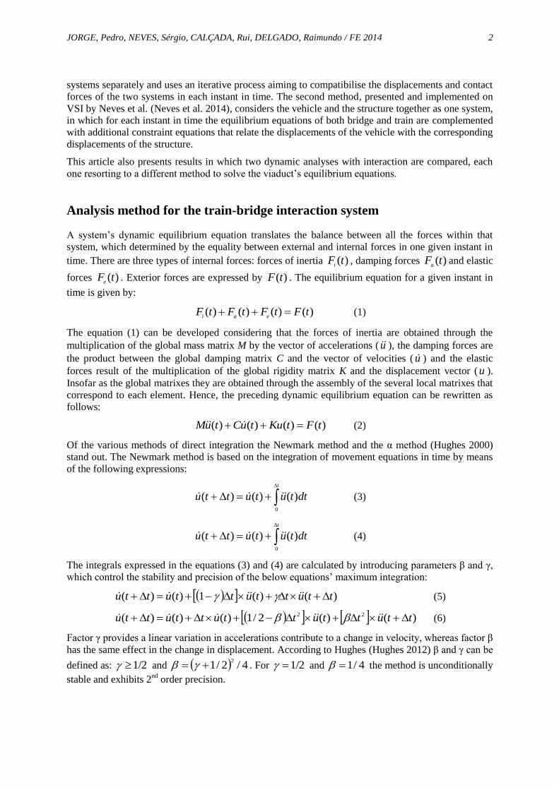
Factor γ provides a linear variation in accelerations contribute to a change in velocity, whereas factor β

has the same effect in the change in displacement. According to Hughes (Hughes 2012) β and γ can be

defined as: 1/2 and 4/2/12

. For 1/2 and 4/1 the method is unconditionally

stable and exhibits 2nd

order precision.


Ribeiro (Ribeiro 2004) has concluded that to achieve a more adequate description of the acceleration

fields on the bridge it would be more correct to obtain the increment in time (∆t) through according to

the following expression:

max20

1

ft (7)

As an alternative to the direct integration methods for solving the differential dynamic equilibrium

equations can resort to the modal superposition method. It is a method based on the decoupling of the

differential equations through transformation of the initial coordinates into modal coordinates. By

doing so, creating linearly independent system of equations, it is possible to study each mode

independently. The separated equation referring to the vibration mode n is obtained by replacing the

general coordinates ( u ) by modal coordinates (n

y ) in the dynamic equilibrium equation. The one

presented is given by (Clough 1993):

)()()()( tFtyKtyCtyMnnnnnnn

(8)

in which n

M represents the modal mass, n

C represents modal damping, n

K represents modal rigidity

and n

F represents modal force. By means of vibration modes’ ortogonality conditions the following is

obtained:

n

T

nnMM

(9)

n

T

nnCC

(10)

n

T

nnKK

(11)

)(tFF T

nn (12)

By solving the equations of equilibrium all the modal coordinates (n

y ) are determined and when the

effects of the modes that intervene in the responses are superposed, the final vector of the final

displacements (u ) of each degree of freedom is calculated.

Iterative method

This method, based on the method presented by Calçada (Calçada 1995), takes into account a dot-line

contact to simulate the contact between wheel and rail. Only the vertical contact forces are considered

and it is assumed that the vehicle’s wheels are in constant contact with the railway. The modelling of

both bridge and train as well as the verification of both of their dynamic equilibrium equations are

done independently. However, the calculation of both structures is done simultaneously, so that

through an iterative process the displacements between bridge and train are made compatible.

Figure 1 illustrates how the compatibilisation between the two subsystems is done resorting to the

iterative method.


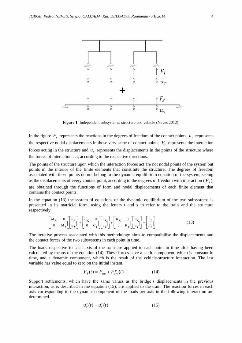
Figure 1. Independent subsystems: structure and vehicle (Neves 2012).

In the figure T

F represents the reactions in the degrees of freedom of the contact points, T

u represents

the respective nodal displacements in those very same of contact points, S

F represents the interaction

forces acting in the structure and S

u represents the displacements in the points of the structure where

the forces of interaction act, according to the respective directions.

The points of the structure upon which the interaction forces act are not nodal points of the system but

points in the interior of the finite elements that constitute the structure. The degrees of freedom

associated with those points do not belong to the dynamic equilibrium equation of the system, seeing

as the displacements of every contact point, according to the degrees of freedom with interaction (S

F ),

are obtained through the functions of form and nodal displacements of each finite element that

contains the contact points.

In the equation (13) the system of equations of the dynamic equilibrium of the two subsystems is

presented in its matricial form, using the letters t and s to refer to the train and the structure

respectively.

TF

SF

Tu

Su

TK

SK

Tu

Su

TC

SC

Tu

Su

TM

SM

0

0

0

0

0

0

(13)

The iterative process associated with this methodology aims to compatibilise the displacements and

the contact forces of the two subsystems in each point in time.

The loads respective to each axis of the train are applied to each point in time after having been

calculated by means of the equation (14). These forces have a static component, which is constant in

time, and a dynamic component, which is the result of the vehicle-structure interaction. The last

variable has value equal to zero on the initial instant.

)()( tFFtF p

dynstaS (14)

Support settlements, which have the same values as the bridge’s displacements in the previous

interaction, as is described in the equation (15), are applied to the train. The reaction forces in each

axis corresponding to the dynamic component of the loads per axis in the following interaction are

determined.

)()( tutu c

S

c

T (15)


In the end of each interaction a convergence criterion that evaluates wether or not the result obtained is

sufficiently precise is described in the equation (16). To that t instant the iterative process is ends when

the convergence criterion has been determined.

tolerancetF

tFtFp

dyn

p

dyn

c

dyn

)(

)()( (16)

Direct method

This methodology was developed by Neves et al. (Neves et al. 2012, Neves et al. 2014) and it allows

the vertical interaction between bridge and train to be analysed in two-dimentional and three-

dimensional problems. In each point in time the dynamic equilibrium equations of the bridge and train

are accompanied by additional displacement compatibility equations that connect the train’s nodal

displacements to the nodal displacements on the bridge. Application of these restrictions is based on

the Lagrange multipliers. The irregularities present in the contact interface may be taken into account

in the compatibility equations. In the method developed by Neves et al. (Neves et al. 2012, Neves et

al. 2014) these equations are only mandatory when the elements are in contact with each other, hence

allowing wheel and rail loss of contact. The dynamic equilibrium equations and the constraint

equations form a single system whose unknowns are the displacements and contact forces. The system

is solved directly without the need to resort to an iterative process to satisfy the compatibility between

the two subsystems. Due to the nonlinear nature of the contact is considered an incremental procedure

based on Newton's method and still using a factoring algorithm block to solve the system of equations.

In Figure 2 the bridge-rail two-dimensional contact used in the present methodology and the local

coordinate system (ξ1, ξ2, ξ3) of the contact pair are represented. ξ2 axis always points in the direction

of the contact node and both elements are separated by an initial gap g. When contact occurs, the

contact node and k node coincide. The contact forces in action are marked as X and the

aforementioned CE and TE indicate the contact element and the target element respectively.

a) b)

Figure 2. Node-to-segment contact element: (a) forces and (b) displacements at the contact interface

(Montenegro et al. 2013)

Forces acting at the contact interface are balanced, therefore:

0 TECE XX (17)


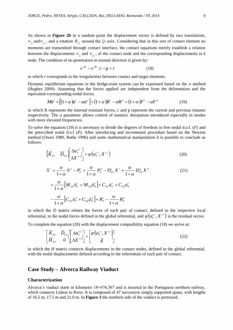
As shown in Figure 2b in a random point the displacement vector is defined by two translations,

1 and

2 , and a rotation

3 around the ξ3 axix. Considering that in this sort of contact element no

moments are transmitted through contact interface, the contact equations merely establish a relation

between the displacements 1

and 2

, of the contact node and the corresponding displacements in k

node. The condition of no penetration in normal direction is given by:

rgTECE (18)

in which r corresponds to the irregularities between contact and target elements.

Dynamic equilibrium equations in the bridge-train system can be expressed based on the α method

(Hughes 2000). Assuming that the forces applied are independent from the deformation and the

equivalent corresponding nodal forces.

pcpcpcc FFRRaaaM 111 (19)

in which R represents the internal resistant forces, c and p represent the current and previous instants

respectively. The α parameter allows control of numeric dissipation introduced especially in modes

with more elevated frequencies.

To solve the equation (19) it is necessary to divide the degrees of freedom in free nodal d.o.f. (F) and

the prescribed nodal d.o.f (P). After introducing and incremental procedure based on the Newton

method (Owen 1980, Bathe 1996) and some mathematical manipulation it is possible to conclude as

follows:

icic

Fi

i

F

FXFFXa

X

aDK ,,

1

1

,

(20)

pp

PX

cc

PX

p

P

c

P

pc XDXDPPSS

111 (21)

c

PPP

c

FPF

c

PPP

c

FPFaCaCaMaM

1

p

P

c

P

p

PPP

p

FPFRRaCaC

11

in which the D matrix relates the forces of each pair of contact, defined in the respective local

referential, to the nodal forces defined in the global referential, and icic

FXa ,, , is the residual vector.

To complete the equation (20) with the displacement compatibility equation (18) we arrive at:

g

Xa

X

a

H

DK icic

F

i

i

F

XF

FXFF

,,

1

1 ,

0

(22)

in which the H matrix connects displacements in the contact nodes, defined in the global referential,

with the nodal displacements defined according to the referentials of each pair of contact.

Case Study – Alverca Railway Viaduct

Characterization

Alverca’s viaduct starts in kilometre 18+676,367 and is inserted in the Portuguese northern railway,

which connects Lisbon to Porto. It is composed of 47 successive simply supported spans, with lengths

of 16.5 m, 17.5 m and 21.0 m. In Figure 3 the northern side of the viaduct is portrayed.


Figure 3. Alverca Viaduct: north side photo

The single-cell box ginger deck consists of a precast U-type beam simple supported by its edges on

pilares and on them sits a system of concrete pre-slabs serving as internal formwork allowing the slab

cast’s in situ concreting. The railway is continuous between successive spans and is made of 30 cm

ballast, monoblock sleepers and UIC60 rails.

Figure 4. Cross section of Alverca railway Viaduct

Numerical modelling of the viaduct

The viaduct’s numeric model is a 3D model of finite elements including the railway, based on the

model created by Fernandes (Fernandes 2010) and Horas (Horas 2011). The dynamic analysis focused

on the first three spans simple supported on the northern side, one of them 16,5 m in length and two of

them 21 m in length, as well as on a 6m ballast extension to simulate the effect of the track on the

embankment. In Figure 5 a global view of the numerical model is shown.


a) b)

Figure 5. Three-dimensional numerical model of Alverca Viaduct in ANSYS: a) Global view and detail of extra

track; b) Cross section

The precast beam, the slab cast and the ballast retaining wall were modelled with Shell elements and

the ballast and the sleepers with elements of volume. Both the ballast enveloping the sleepers as well

as the edge beams were modelled with concentrated masses. Between the rail and the sleeper springs

of rigidity similar to that of the pads were used. Aditional elements that apply constraint equations

were also considered to guarantee the compatibilisation of the displacements between the several

disconnected elements.

The numerical model of the Alverca’s viaduct has already been calibrated once through the results of

ambient vibration tests. These results led to the identification of several modal parameters, like

vibration modes, natural frequencies and damping coefficients. All the post calibration geometric and

mechanic characteristics of the model can be observed in the article of Malveiro et al. (Malveiro et al.

2012).

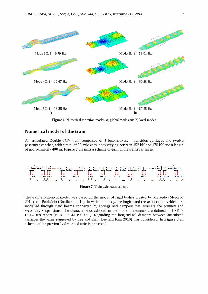
In Figure 6 the global vibration modes of the deck (G) and the local vibration modes of the upper

slabs and the consoles obtained from the post calibration vibration model are displayed.

Mode 1G: f = 6.73 Hz Mode 1L: f = 26.68 Hz






a) b)

Figure 6. Numerical vibration modes: a) global modes and b) local modes

Numerical model of the train

An articulated Double TGV train comprised of 4 locomotives, 4 transition carriages and twelve

passenger coaches, with a total of 52 axle with loads varying between 153 kN and 170 kN and a length

of approximately 400 m. Figure 7 presents a scheme of each of the trains carriages.

Figure 7. Train axle loads scheme

The train’s numerical model was based on the model of rigid bodies created by Meixedo (Meixedo

2012) and Bonifácio (Bonifácio 2012), in which the body, the bogies and the axles of the vehicle are

modelled through rigid beams connected by springs and dampers that simulate the primary and

secondary suspensions. The characteristics adopted in the model’s elements are defined in ERRI’s

D214/RP9 report (ERRI D214/RP9 2001). Regarding the longitudinal dampers between articulated

carriages the value suggested by Lee and Kim (Lee and Kim 2010) was considered. In Figure 8 an

scheme of the previously described train is presented.


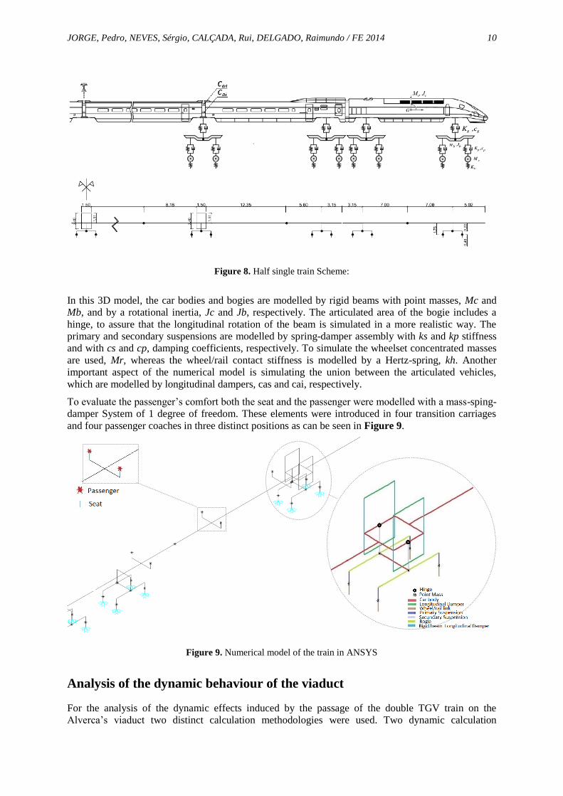
Figure 8. Half single train Scheme:

In this 3D model, the car bodies and bogies are modelled by rigid beams with point masses, Mc and

Mb, and by a rotational inertia, Jc and Jb, respectively. The articulated area of the bogie includes a

hinge, to assure that the longitudinal rotation of the beam is simulated in a more realistic way. The

primary and secondary suspensions are modelled by spring-damper assembly with ks and kp stiffness

and with cs and cp, damping coefficients, respectively. To simulate the wheelset concentrated masses

are used, Mr, whereas the wheel/rail contact stiffness is modelled by a Hertz-spring, kh. Another

important aspect of the numerical model is simulating the union between the articulated vehicles,

which are modelled by longitudinal dampers, cas and cai, respectively.

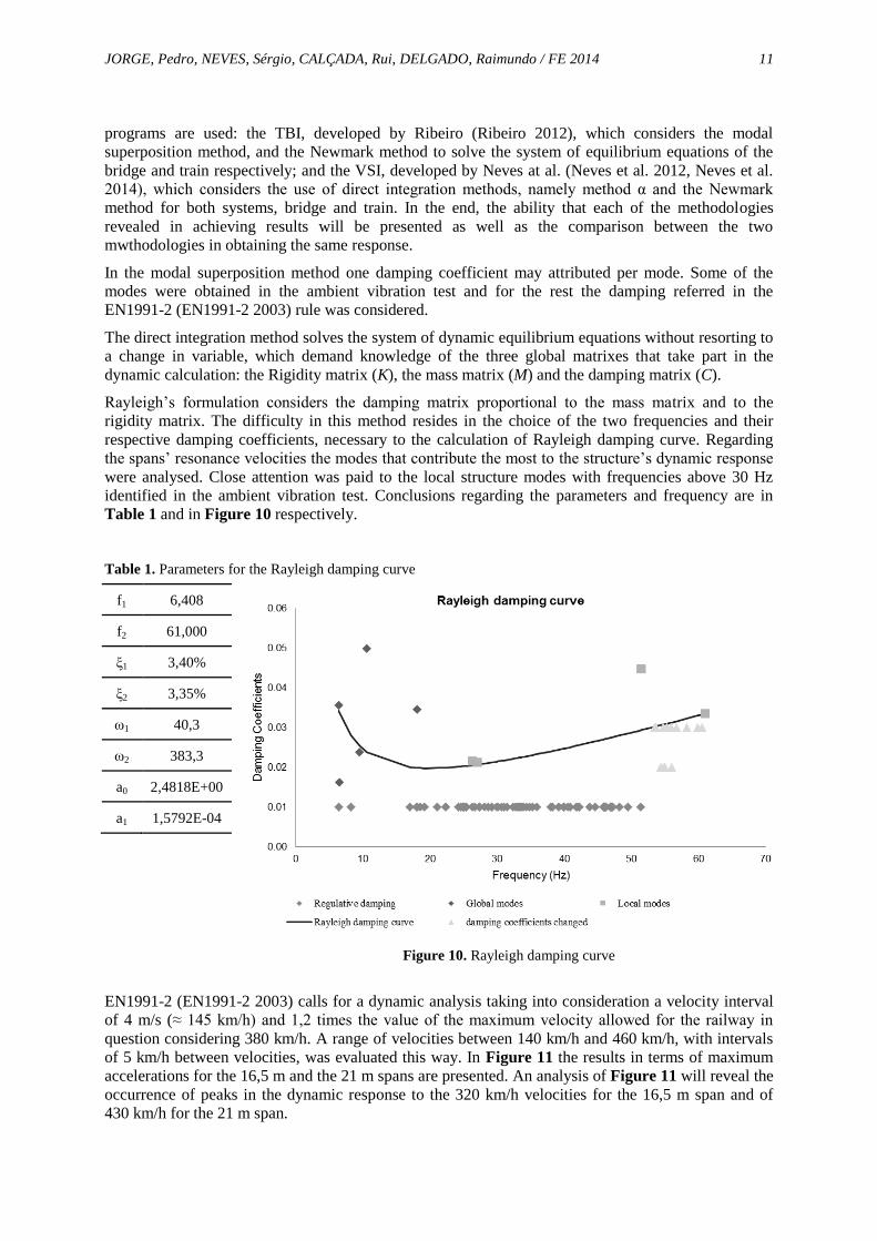
To evaluate the passenger’s comfort both the seat and the passenger were modelled with a mass-sping-

damper System of 1 degree of freedom. These elements were introduced in four transition carriages

and four passenger coaches in three distinct positions as can be seen in Figure 9.

Figure 9. Numerical model of the train in ANSYS

Analysis of the dynamic behaviour of the viaduct

For the analysis of the dynamic effects induced by the passage of the double TGV train on the

Alverca’s viaduct two distinct calculation methodologies were used. Two dynamic calculation


programs are used: the TBI, developed by Ribeiro (Ribeiro 2012), which considers the modal

superposition method, and the Newmark method to solve the system of equilibrium equations of the

bridge and train respectively; and the VSI, developed by Neves at al. (Neves et al. 2012, Neves et al.

2014), which considers the use of direct integration methods, namely method α and the Newmark

method for both systems, bridge and train. In the end, the ability that each of the methodologies

revealed in achieving results will be presented as well as the comparison between the two

mwthodologies in obtaining the same response.

In the modal superposition method one damping coefficient may attributed per mode. Some of the

modes were obtained in the ambient vibration test and for the rest the damping referred in the

EN1991-2 (EN1991-2 2003) rule was considered.

The direct integration method solves the system of dynamic equilibrium equations without resorting to

a change in variable, which demand knowledge of the three global matrixes that take part in the

dynamic calculation: the Rigidity matrix (K), the mass matrix (M) and the damping matrix (C).

Rayleigh’s formulation considers the damping matrix proportional to the mass matrix and to the

rigidity matrix. The difficulty in this method resides in the choice of the two frequencies and their

respective damping coefficients, necessary to the calculation of Rayleigh damping curve. Regarding

the spans’ resonance velocities the modes that contribute the most to the structure’s dynamic response

were analysed. Close attention was paid to the local structure modes with frequencies above 30 Hz

identified in the ambient vibration test. Conclusions regarding the parameters and frequency are in

Table 1 and in Figure 10 respectively.

Table 1. Parameters for the Rayleigh damping curve

f1 6,408

f2 61,000

ξ1 3,40%

ξ2 3,35%

ω1 40,3

ω2 383,3

a0 2,4818E+00

a1 1,5792E-04

Figure 10. Rayleigh damping curve

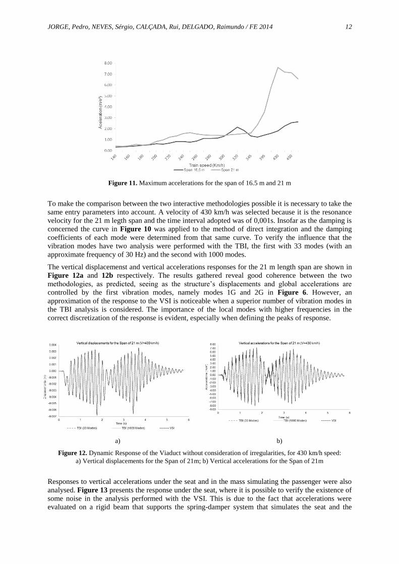
EN1991-2 (EN1991-2 2003) calls for a dynamic analysis taking into consideration a velocity interval

of 4 m/s (≈ 145 km/h) and 1,2 times the value of the maximum velocity allowed for the railway in

question considering 380 km/h. A range of velocities between 140 km/h and 460 km/h, with intervals

of 5 km/h between velocities, was evaluated this way. In Figure 11 the results in terms of maximum

accelerations for the 16,5 m and the 21 m spans are presented. An analysis of Figure 11 will reveal the

occurrence of peaks in the dynamic response to the 320 km/h velocities for the 16,5 m span and of

430 km/h for the 21 m span.


Figure 11. Maximum accelerations for the span of 16.5 m and 21 m

To make the comparison between the two interactive methodologies possible it is necessary to take the

same entry parameters into account. A velocity of 430 km/h was selected because it is the resonance

velocity for the 21 m legth span and the time interval adopted was of 0,001s. Insofar as the damping is

concerned the curve in Figure 10 was applied to the method of direct integration and the damping

coefficients of each mode were determined from that same curve. To verify the influence that the

vibration modes have two analysis were performed with the TBI, the first with 33 modes (with an

approximate frequency of 30 Hz) and the second with 1000 modes.

The vertical displacemenst and vertical accelerations responses for the 21 m length span are shown in

Figure 12a and 12b respectively. The results gathered reveal good coherence between the two

methodologies, as predicted, seeing as the structure’s displacements and global accelerations are

controlled by the first vibration modes, namely modes 1G and 2G in Figure 6. However, an

approximation of the response to the VSI is noticeable when a superior number of vibration modes in

the TBI analysis is considered. The importance of the local modes with higher frequencies in the

correct discretization of the response is evident, especially when defining the peaks of response.

a) b)

Figure 12. Dynamic Response of the Viaduct without consideration of irregularities, for 430 km/h speed:

a) Vertical displacements for the Span of 21m; b) Vertical accelerations for the Span of 21m

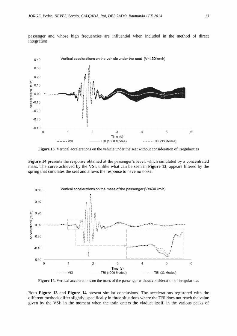
Responses to vertical accelerations under the seat and in the mass simulating the passenger were also

analysed. Figure 13 presents the response under the seat, where it is possible to verify the existence of

some noise in the analysis performed with the VSI. This is due to the fact that accelerations were

evaluated on a rigid beam that supports the spring-damper system that simulates the seat and the


passenger and whose high frequencies are influential when included in the method of direct

integration.

Figure 13. Vertical accelerations on the vehicle under the seat without consideration of irregularities

Figure 14 presents the response obtained at the passenger’s level, which simulated by a concentrated

mass. The curve achieved by the VSI, unlike what can be seen in Figure 13, appears filtered by the

spring that simulates the seat and allows the response to have no noise.

Figure 14. Vertical accelerations on the mass of the passenger without consideration of irregularities

Both Figure 13 and Figure 14 present similar conclusions. The accelerations registered with the

different methods differ slightly, specifically in three situations where the TBI does not reach the value

given by the VSI: in the moment when the train enters the viaduct itself, in the various peaks of


response and also in the moment when the train exits the bridge. In these situations the number of

modes used in the modal superposition method rise to become important in the sense that the response

has a tendency to get closer to the response achieved by the direct integration method. Unlike the 21 m

length span’s vertical displacements whose final response was described in full by the first modes,

when it comes to accelerations the more elevated modes become particularly important to describe

specific response situations, of which the three aforementioned situations are example. In the case of

accelerations under the seat and on the mass of the passenger the modal superposition method falls

short because it doesn’t consider the impact of the deformation of the railway, which is characterised

by modes with higher frequencies. In Figure 14 an enlargement of the moment when the vehicle

enters the viaduct is performed in which the approximation of the response by the TBI is observed

when the number of modes considered is superior by 30.

In the dynamic analyses that involve vehicle-structure interaction the irregularities in the railway were

considered. The conclusions drawn from the responses are absolutely similar to those drawn from the

analyses that didn’t observe the irregularities in the railway.

By looking at Figure 15 one can see that taking railway irregularities into account significantly affects

accelerations measured within the vehicle, with an approximate twofold increase in accelerations.

Because of this, to verify the level of comfort for the passenger it is essential to consider irregularities.

Rule EN1990-2 (EN1991-2 2003) indicates the limit of maximum vertical acceleration to which the

carriage may be subjected from 1 m/s² to a very good level of comfort. A value close to 0,70 m/s² was

achieved, under 1 m/s², which allowed the criterion to be met.

a) b)

Figure 15. Dynamic Response of the Train considering irregularities, for 430 km/h speed:

a) Vertical accelerations on the vehicle under the seat; b) Vertical accelerations on the mass of the passenger

Conclusions

The present article evolved towards evaluating the dynamic effects of the passage of a train like the

TGV on the Alverca’s viaduct. Applying two analysis methodologies involving vehicle-structure

interaction requires the modelling of both parts. Modelling that was based on models created by other

authors.

Before the comparison dynamic analyses between the two methods were performed it was essential

that both entry parameter were the same. At this point the major difficulty was to adapt a damping

curve to the types of damping seen in each mode, set between regulative damping and experimentally

measured damping.

An analysis for a velocity close to the resonance velocity for the 21 m length span was performed,

considering modal dampings collected from Rayleigh’s damping curve. Two additional analyses were

also performed with the TBI: the first took the 33 vibration modes into account and the second took

the 1000 vibration modes into consideration so that the importance of the number of modes would

become clear in the final response. Analyses in terms of displacements and accelerations proved to be


close to one another, leading to the conclusion that the analysis is mainly determined by lower

frequency modes, associated with modes that involve the global deformation of the structure.

Regarding the responses gathered for the passenger and under the seat differences in the results were

confirmed, especially in three situations: in the moment when the train enters the viaduct itself, in the

peaks of response and also in the viaduct’s exiting area. The differences observed also display an

approximation of the TBI’s response when a higher number of vibration modes is considered. These

differences exist because the TBI ignores the deformation of the railway, which is usually presents

higher frequencies.

The existence of irregularities in the Railway, which have an important role in dynamic analysis

because they make the calculation more realistic was also considered in the analysis. In this way, the

influence of this parameter in the interaction analysis and the differences present in the two dynamic

analysis methodologies considered were evaluated. By looking at the results from within the train it is

explicitly notorious that the registered maximum acceleration values increase when irregularities in the

railway are considered. It was also concluded that the passengers’ level of comfort is very good in the

scenario where irregularities in the railway are considered and the train is travelling with velocity

closer to the ressonat fot the 21 m span.

References

Bathe, K. J. (1996). Finite element procedures. Upper Saddle River, NJ, Prentice-Hall.

Calçada, R. A. B., Efeitos dinâmicos em pontes resultantes do tráfego ferroviário a alta velocidade,

Master Thesis, FEUP, Porto, 1995.

Clough, R. W., Penzien, J. (1993). Dynamics of structures, McGraw-Hill New York.

EN1991-2, Eurocode 1: Actions on structures - Part 2: Traffic loads on Bridges, 2003, European

Committee for Standardization (CEN): Brussels, Belgium.

ERRI D214/RP9, Rail bridges for speeds > 200 Km/h final report ERRI D 214/RP 9, 2001, European

Rail Research Institute: Utrecht, Netherlands.

Fernandes, M. A. M., Comportamento dinâmico de pontes com tabuleiro pré-fabricado em vias de

alta velocidade, Master Thesis, FEUP, Porto, 2010.

Horas, C. C. S., Comportamento dinâmico de pontes com tabuleiro pré-fabricado em vias de alta

velocidade, Master Thesis, FEUP, Porto, 2011.

Hughes, T. J. R. (2000). The finite element method: Linear static and dynamic finite element analysis.

New York, Dover Publications.

Hughes, T. J. R. (2012). The finite element method: linear static and dynamic finite element analysis,

Courier Dover Publications.

Lee, Y.-S. and Kim, S.-H. (2010) Structural analysis of 3D high-speed train–bridge interactions for

simple train load models. Vehicle System Dynamics. 48(2): p. 263-281.

Malveiro, J., Ribeiro, D. R. F., Sousa, C. and Calçada, R. A. B. (2012) Updating and validation of the

dynamic model of a railway viaduct with precast deck.

Montenegro, P. A., Neves, S. G. M., Azevedo, A. F. M. and Calçada, R. A. B., A nonlinear vehicle-

structure interaction methodology with wheel-rail detachment and reattachment, in 4th

ECCOMAS Thematic Conference on Computational Methods in Structural Dynamics and

Earthquake Engineering2013, COMPDYN 2013: Kos Island, Greece.

Neves, S. G. M., Análise dinâmica com interacção veículo-estrutura em vias de alta velocidade,

Master Thesis, FEUP, 2012.


Neves, S. G. M., Azevedo, A. F. M. and Calçada, R. A. B. (2012) A direct method for analyzing the

vertical vehicle–structure interaction. Engineering Structures. 34: p. 414-420.

Neves, S. G. M., Montenegro, P. A., Azevedo, A. F. M. and Calçada, R. (2014) A direct method for

analyzing the nonlinear vehicle–structure interaction. Engineering Structures. 69: p. 83-89.

Owen, D. R. J., Hinton, E. (1980). Finite Elements in Plasticity: Theory and Practice. Swansea, UK,

Pineridge Press Limited.

Ribeiro, D. R. F., Comportamento dinâmico de pontes sob acção de tráfego ferroviário a alta

velocidade, Dissertação para obtenção do grau de Mestre em Engenharia Civil, FEUP, Porto,

2004.

Ribeiro, D. R. F., Efeitos dinâmicos induzidos por tráfego em pontes ferroviárias modelação

numérica, calibração e validação experimental, Doctoral Thesis, FEUP, Porto, 2012.

Date post:	24-Jan-2019
Category:	Documents
Upload:	lamnhu
View:	214 times
Download:	0 times

Dynamic Behaviour of a Railway Viaduct with a Precast Deck … · JORGE, Pedro, NEVES, Sérgio,...

Documents