Dynamic Causal Modelling (DCM) for fMRI

Klaas Enno Stephan

Laboratory for Social & Neural Systems Research (SNS) University of Zurich

Wellcome Trust Centre for NeuroimagingUniversity College London

SPM Course, FIL13 May 2011

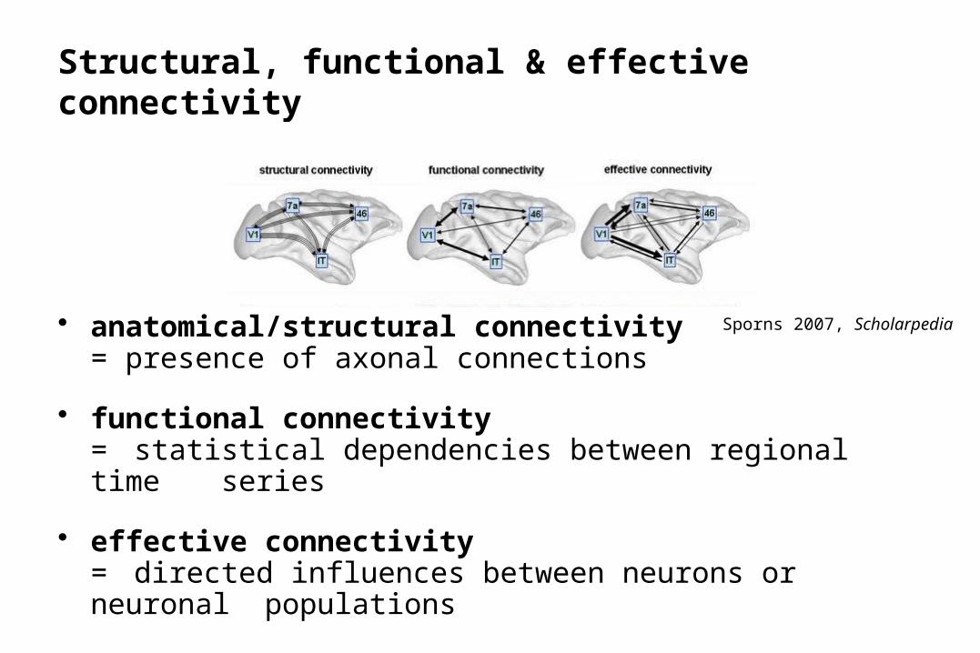
Structural, functional & effective connectivity

• anatomical/structural connectivity= presence of axonal connections

• functional connectivity = statistical dependencies between regional time series

• effective connectivity = directed influences between neurons or neuronal populations

Sporns 2007, Scholarpedia

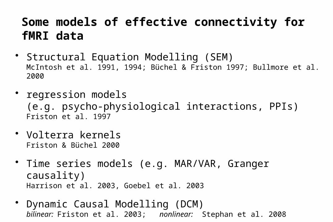
Some models of effective connectivity for fMRI data

• Structural Equation Modelling (SEM) McIntosh et al. 1991, 1994; Büchel & Friston 1997; Bullmore et al. 2000

• regression models (e.g. psycho-physiological interactions, PPIs)Friston et al. 1997

• Volterra kernels Friston & Büchel 2000

• Time series models (e.g. MAR/VAR, Granger causality)Harrison et al. 2003, Goebel et al. 2003

• Dynamic Causal Modelling (DCM)bilinear: Friston et al. 2003; nonlinear: Stephan et al. 2008

Dynamic causal modelling (DCM)

• DCM framework was introduced in 2003 for fMRI by Karl Friston, Lee Harrison and Will Penny (NeuroImage 19:1273-1302)

• part of the SPM software package

• currently more than 160 published papers on DCM

),,( uxFdt

dx

Neural state equation:

Electromagneticforward model:

neural activityEEGMEGLFP

Dynamic Causal Modeling (DCM)

simple neuronal modelcomplicated forward model

complicated neuronal modelsimple forward model

fMRIfMRI EEG/MEGEEG/MEG

inputs

Hemodynamicforward model:neural activityBOLD

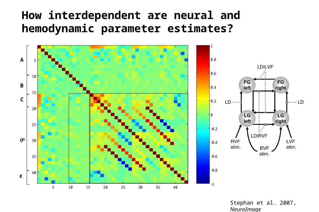
LGleft

LGright

RVF LVF

FGright

FGleft

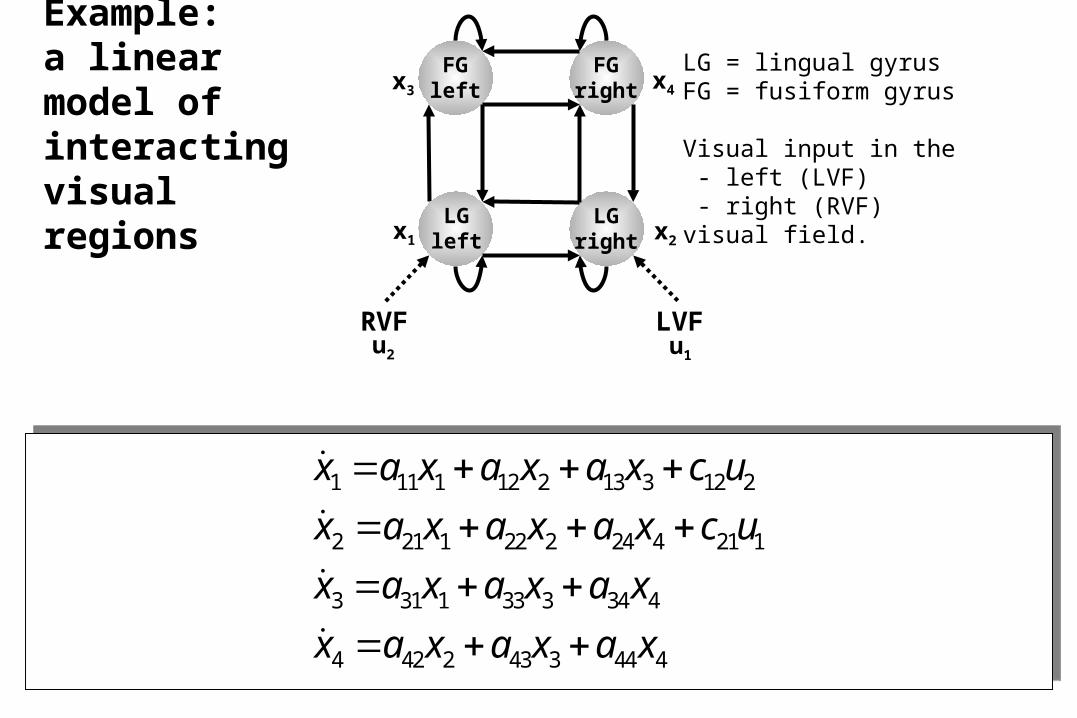
LG = lingual gyrusFG = fusiform gyrus

Visual input in the - left (LVF) - right (RVF)visual field.x1 x2

x4x3

u2 u1

1 11 1 12 2 13 3 12 2

2 21 1 22 2 24 4 21 1

3 31 1 33 3 34 4

4 42 2 43 3 44 4

x a x a x a x c u

x a x a x a x c u

x a x a x a x

x a x a x a x

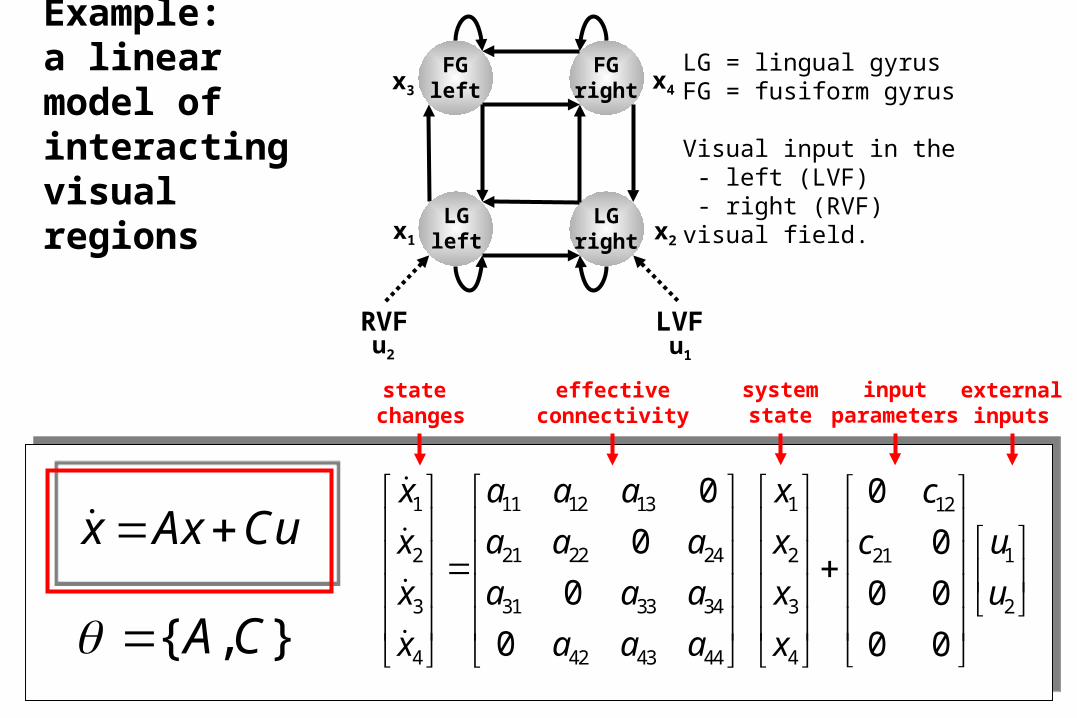
Example: a linear model of interacting visual regions

Example: a linear model of interacting visual regions

LG = lingual gyrusFG = fusiform gyrus

Visual input in the - left (LVF) - right (RVF)visual field.

state changes

effectiveconnectivity

externalinputs

systemstate

inputparameters

11 12 131 1 12

21 22 242 2 121

31 33 343 3 2

42 43 444 4

0 0

0 0

0 0 0

0 0 0

a a ax x c

a a ax x uc

a a ax x u

a a ax x

x Ax Cu

},{ CA

LGleft

LGright

RVF LVF

FGright

FGleft

x1 x2

x4x3

u2 u1

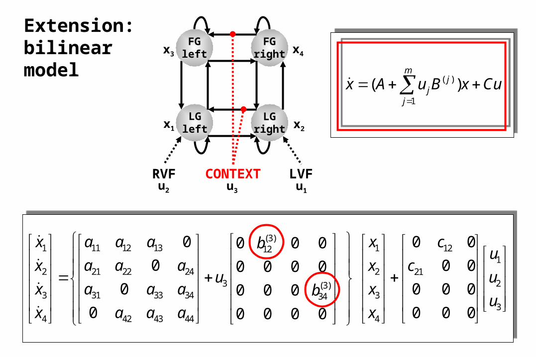
Extension: bilinear model

LGleft

LGright

RVF LVF

FGright

FGleft

x1 x2

x4x3

u2 u1

CONTEXTu3

( )

1

( )m

jj

j

x A u B x Cu

(3)11 12 131 1 1212

121 22 242 2 21

3 2(3)31 33 343 334

342 43 444 4

0 0 00 0 0

0 0 00 0 0 0

0 0 0 00 0 0

0 0 0 00 0 0 0

a a ax x cbu

a a ax x cu u

a a ax xbu

a a ax x

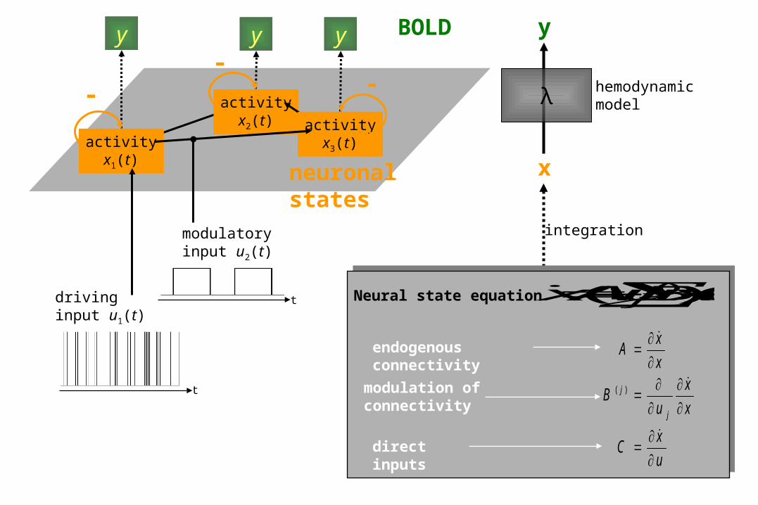
endogenous connectivity

direct inputs

modulation ofconnectivity

Neural state equation CuxBuAx jj )( )(

u

xC

x

x

uB

x

xA

j

j

)(

hemodynamicmodelλ

x

y

integration

BOLDyyy

activityx1(t)

activityx2(t) activity

x3(t)

neuronalstates

t

drivinginput u1(t)

modulatoryinput u2(t)

t

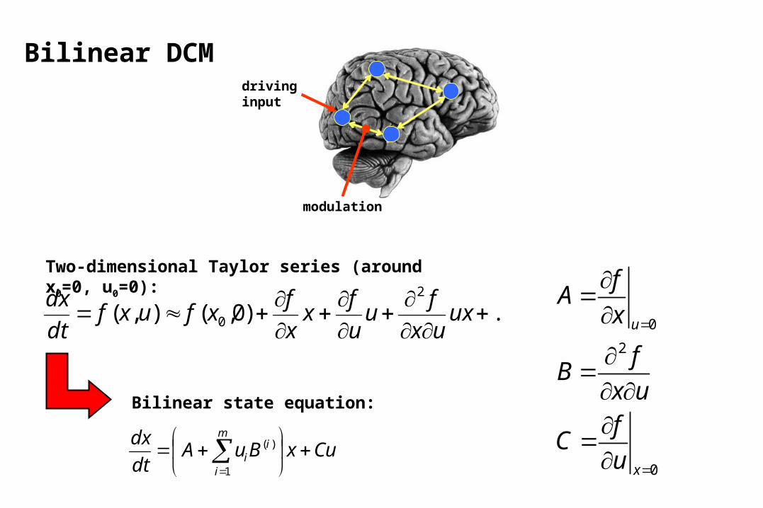
Bilinear DCM

CuxBuAdt

dx m

i

ii

1

)(

Bilinear state equation:

driving input

modulation

...)0,(),(2

0

uxux

fu

u

fx

x

fxfuxf

dt

dx

Two-dimensional Taylor series (around x0=0, u0=0):

0

2

0

u

x

fA

x

fB

x uf

Cu

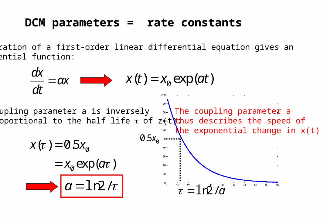
DCM parameters = rate constants

dxax

dt 0( ) exp( )x t x at

The coupling parameter a thus describes the speed ofthe exponential change in x(t)

0

0

( ) 0.5

exp( )

x x

x a

Integration of a first-order linear differential equation gives anexponential function:

/2lna

00.5x

a/2ln

Coupling parameter a is inverselyproportional to the half life of z(t):

-

x2

stimuliu1

contextu2

x1

+

+

-

-

-+

u1

Z1

u2

Z2

2 1

(2)

2121 1111

22

212 222

0 0

0 00

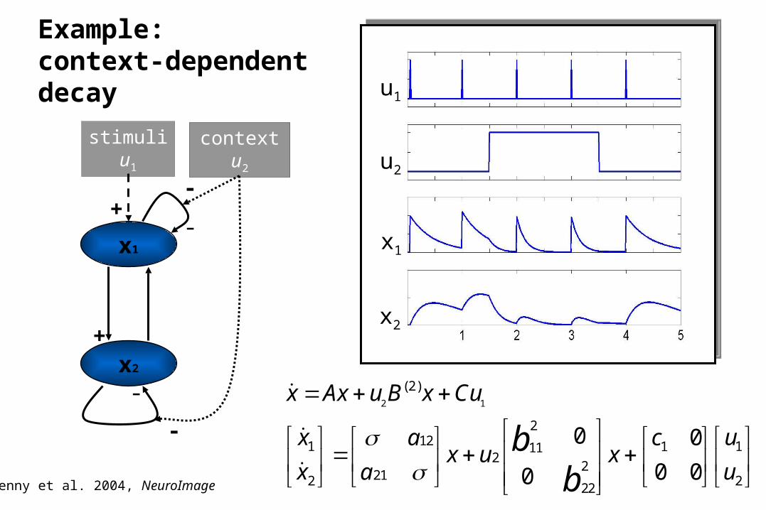
x Ax u B x Cu

x ua cx u x

x uab

b

Example: context-dependent decay u1

u2

x2

x1

Penny et al. 2004, NeuroImage

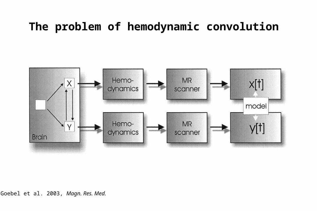
The problem of hemodynamic convolution

Goebel et al. 2003, Magn. Res. Med.

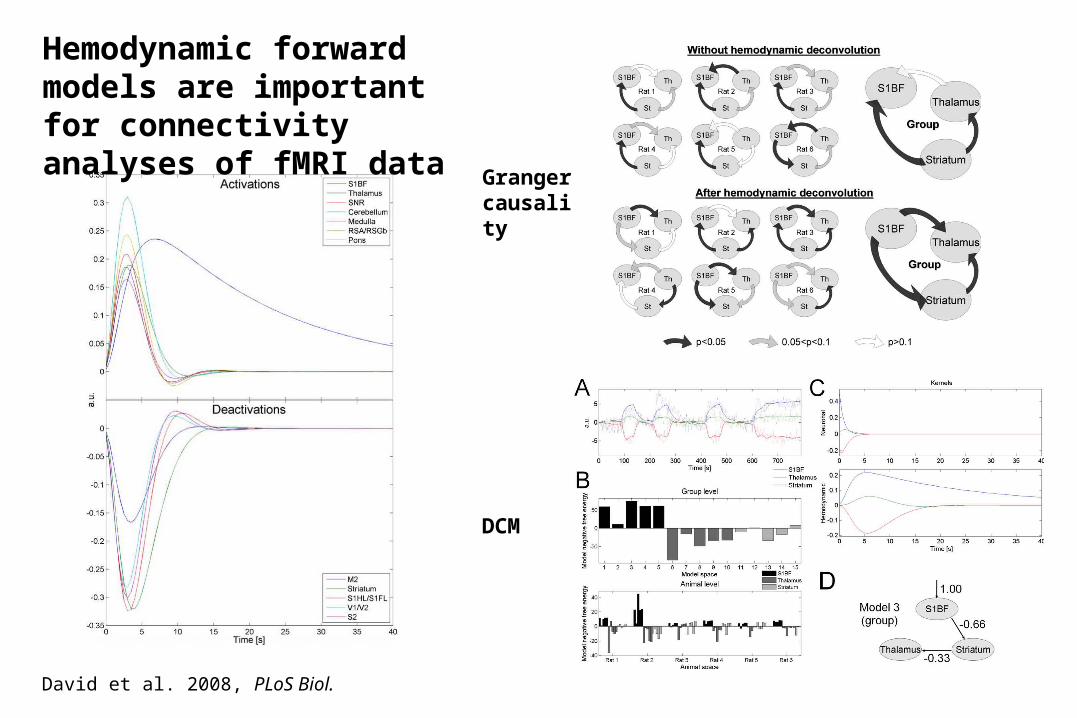
Hemodynamic forward models are important for connectivity analyses of fMRI data

David et al. 2008, PLoS Biol.

Granger causality

DCM

0 2 4 6 8 10 12 14

0

0.2

0.4

0 2 4 6 8 10 12 14

0

0.5

1

0 2 4 6 8 10 12 14

-0.6

-0.4

-0.2

0

0.2

RBMN

, = 0.5

CBMN

, = 0.5

RBMN

, = 1

CBMN

, = 1

RBMN

, = 2

CBMN

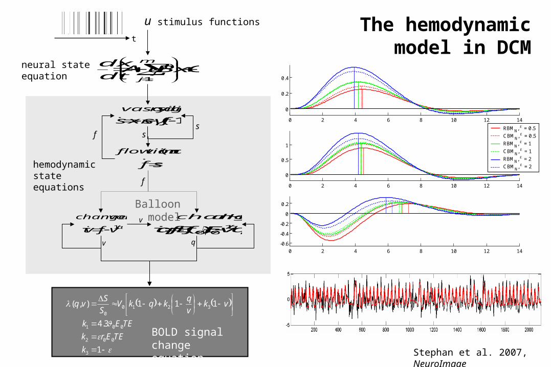
, = 2sf

tionflow induc

(rCBF)

s

v

stimulus functions

v

q q/vvEf,EEfqτ /α

dHbchanges in

100 )( /αvfvτ

volumechanges in

1

f

q

)1(

fγsxs

signalryvasodilato

u

s

CuxBuAdt

dx m

j

jj

1

)(

t

neural state equation

1

3.4

111),(

3

002

001

32100

k

TEErk

TEEk

vkv

qkqkV

S

Svq

hemodynamic state equations

f

Balloon model

BOLD signal change equation

The hemodynamic model in DCM

Stephan et al. 2007, NeuroImage

5 10 15 20 25 30 35 40

5

10

15

20

25

30

35

40

-1

-0.8

-0.6

-0.4

-0.2

0

0.2

0.4

0.6

0.8

1

A

B

C

h

ε

How interdependent are neural and hemodynamic parameter estimates?

Stephan et al. 2007, NeuroImage

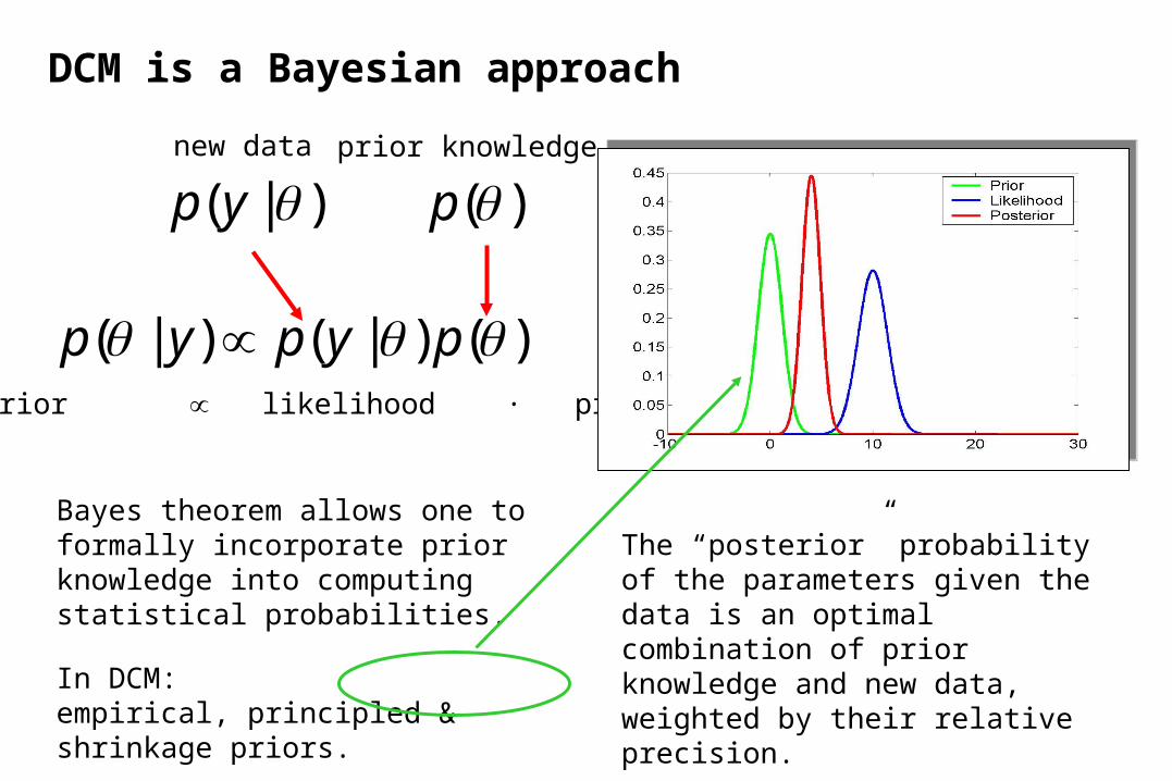
DCM is a Bayesian approach

)()|()|( pypyp posterior likelihood ∙ prior

)|( yp )(p

Bayes theorem allows one to formally incorporate prior knowledge into computing statistical probabilities.

In DCM: empirical, principled & shrinkage priors.

The “posterior” probability of the parameters given the data is an optimal combination of prior knowledge and new data, weighted by their relative precision.

new data prior knowledge

sf (rCBF)induction -flow

s

v

f

stimulus function u

modelled BOLD response

vq q/vvf,Efqτ /α1)(

dHbin changes

/αvfvτ 1

in volume changes

f

q

)1(

signalry vasodilatodependent -activity

fγszs

s

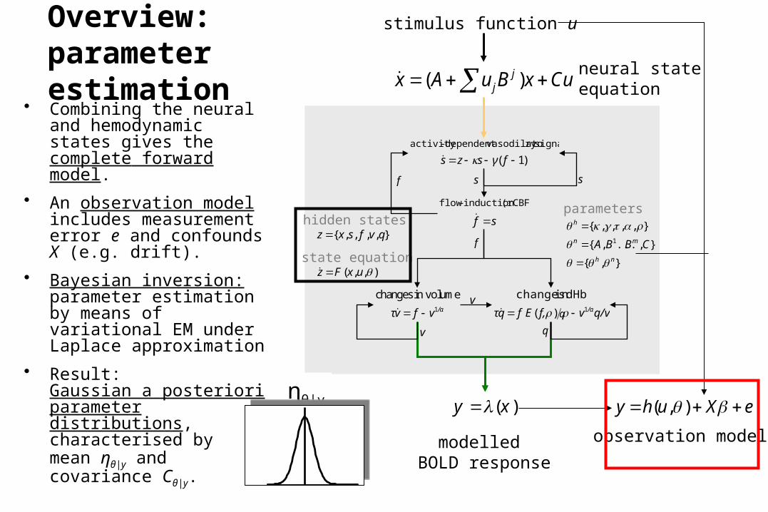
)(xy eXuhy ),(

observation model

hidden states{ , , , , }z x s f v q

state equation( , , )z F x u

parameters

},{

},...,{

},,,,{1

nh

mn

h

CBBA

• Combining the neural and hemodynamic states gives the complete forward model.

• An observation model includes measurement error e and confounds X (e.g. drift).

• Bayesian inversion: parameter estimation by means of variational EM under Laplace approximation

• Result:Gaussian a posteriori parameter distributions, characterised by mean ηθ|y and covariance Cθ|y.

Overview:parameter estimation

ηθ|y

neural stateequation( )j

jx A u B x Cu

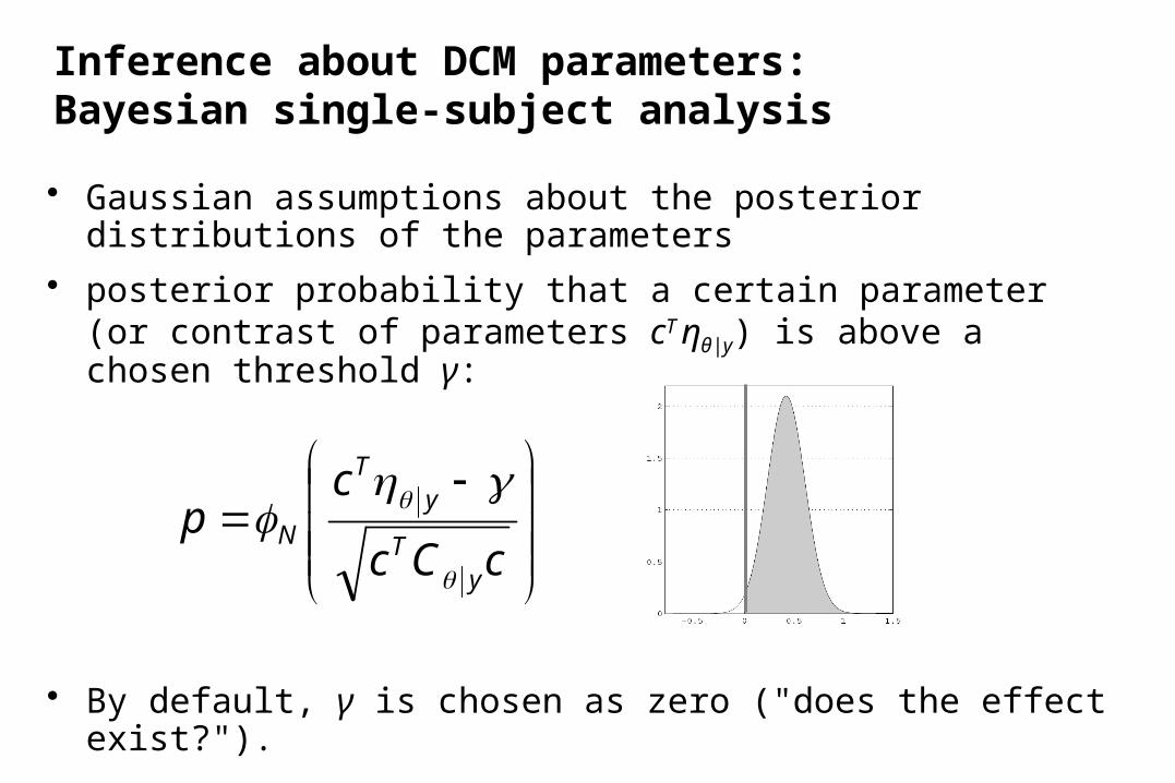
• Gaussian assumptions about the posterior distributions of the parameters

• posterior probability that a certain parameter (or contrast of parameters cT ηθ|y) is above a chosen threshold γ:

• By default, γ is chosen as zero ("does the effect exist?").

Inference about DCM parameters:Bayesian single-subject analysis

cCc

cp

yT

yT

N

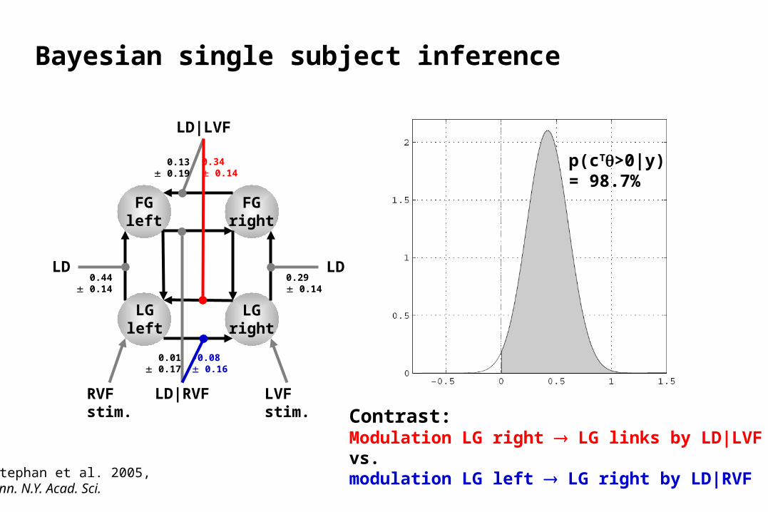
Bayesian single subject inference

LGleft

LGright

RVFstim.

LVFstim.

FGright

FGleft

LD|RVF

LD|LVF

LD LD

0.34 0.14

-0.08 0.16

0.13 0.19

0.01 0.17

0.44 0.14

0.29 0.14

Contrast:Modulation LG right LG links by LD|LVFvs.modulation LG left LG right by LD|RVF

p(cT>0|y) = 98.7%

Stephan et al. 2005, Ann. N.Y. Acad. Sci.

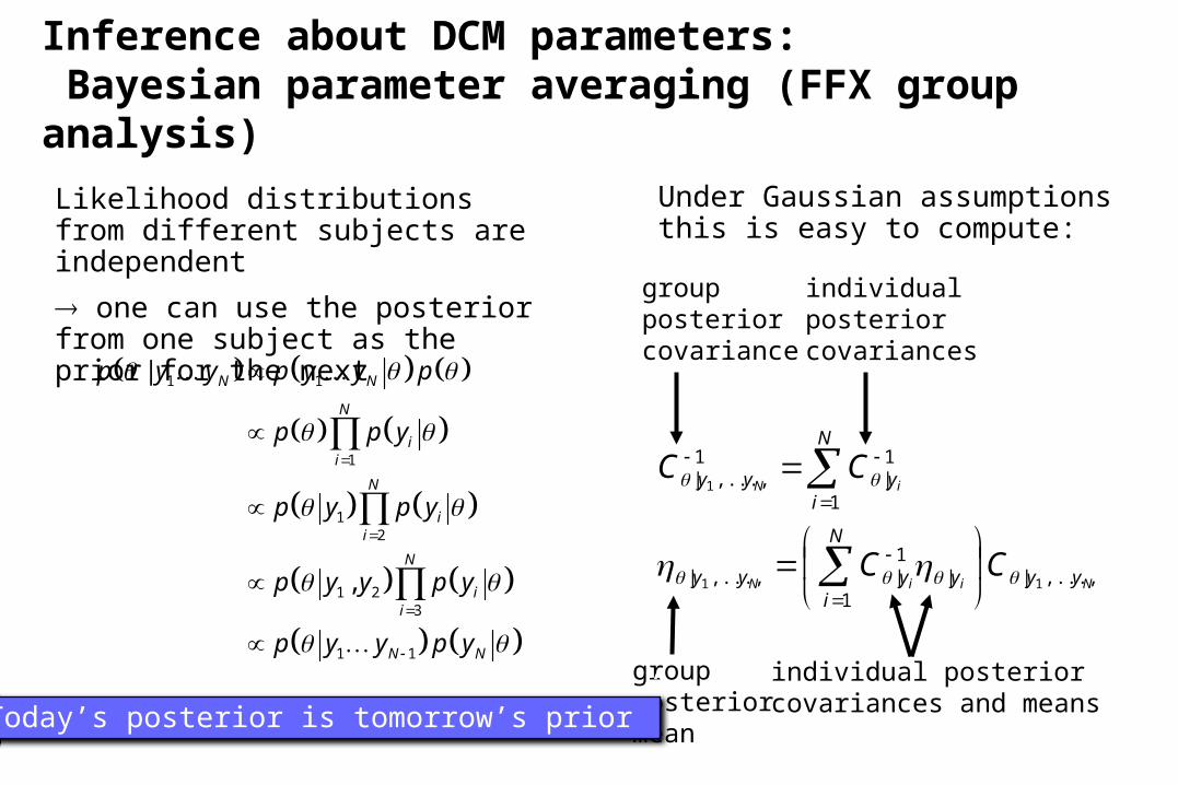
Likelihood distributions from different subjects are independent

one can use the posterior from one subject as the prior for the next

NiiN

iN

yy

N

iyyyy

N

iyyy

CC

CC

,...,|1

|1|,...,|

1

1|

1,...,|

11

1

Under Gaussian assumptions this is easy to compute:

groupposterior covariance

individualposterior covariances

groupposterior mean

individual posterior covariances and means“Today’s posterior is tomorrow’s prior”

Inference about DCM parameters: Bayesian parameter averaging (FFX group analysis)

1 1

1

12

1 23

1 1

|

,

N N

N

ii

N

ii

N

ii

N N

p y y p y y p

p p y

p y p y

p y y p y

p y y p y

Inference about DCM parameters:RFX group analysis (frequentist)

• In analogy to “random effects” analyses in SPM, 2nd level analyses can be applied to DCM parameters:

Separate fitting of identical models for each subject

Separate fitting of identical models for each subject

Selection of (bilinear) parameters of interestSelection of (bilinear) parameters of interest

one-sample t-test:

parameter > 0 ?

one-sample t-test:

parameter > 0 ?

paired t-test: parameter 1 > parameter 2 ?

paired t-test: parameter 1 > parameter 2 ?

rmANOVA: e.g. in case of

multiple sessions per subject

rmANOVA: e.g. in case of

multiple sessions per subject

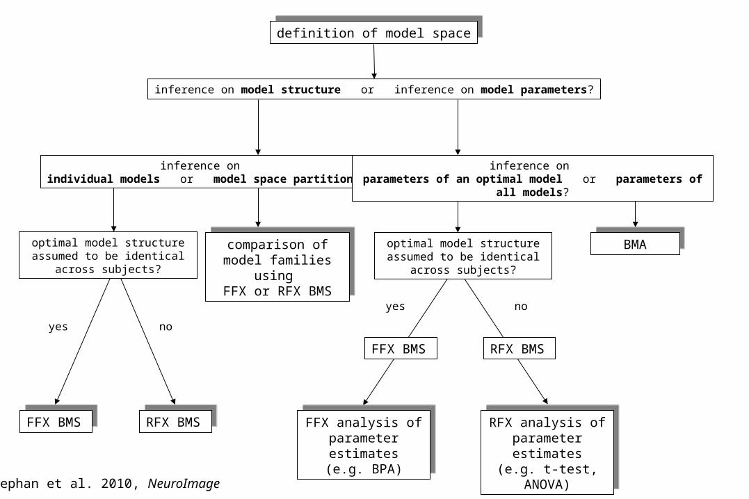
inference on model structure or inference on model parameters?

inference on individual models or model space partition?

comparison of model families using

FFX or RFX BMS

comparison of model families using

FFX or RFX BMS

optimal model structure assumed to be identical across subjects?

FFX BMSFFX BMS RFX BMSRFX BMS

yes no

inference on parameters of an optimal model or parameters of all models?

BMABMA

definition of model spacedefinition of model space

FFX analysis of parameter estimates

(e.g. BPA)

FFX analysis of parameter estimates

(e.g. BPA)

RFX analysis of parameter estimates(e.g. t-test, ANOVA)

RFX analysis of parameter estimates(e.g. t-test, ANOVA)

optimal model structure assumed to be identical across subjects?

FFX BMS

yes no

RFX BMS

Stephan et al. 2010, NeuroImage

Any design that is good for a GLM of fMRI data.

What type of design is good for DCM?

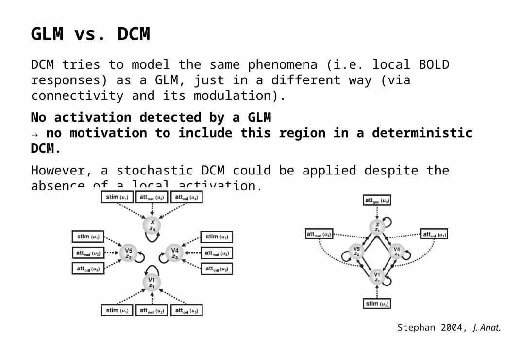
GLM vs. DCM

DCM tries to model the same phenomena (i.e. local BOLD responses) as a GLM, just in a different way (via connectivity and its modulation).

No activation detected by a GLM → no motivation to include this region in a deterministic DCM.

However, a stochastic DCM could be applied despite the absence of a local activation.

Stephan 2004, J. Anat.

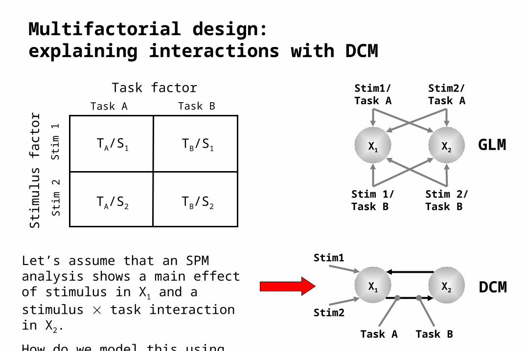
Multifactorial design: explaining interactions with DCM

Task factorTask A Task B

Sti

m 1

Sti

m 2

Sti

mu

lus

fact

or

TA/S1 TB/S1

TA/S2 TB/S2

X1 X2

Stim2/Task A

Stim1/Task A

Stim 1/Task B

Stim 2/Task B

GLM

X1 X2

Stim2

Stim1

Task A Task B

DCM

Let’s assume that an SPM analysis shows a main effect of stimulus in X1 and a stimulus task interaction in X2.

How do we model this using DCM?

Stim 1Task A

Stim 2Task A

Stim 1Task B

Stim 2Task B

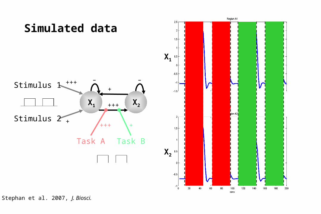
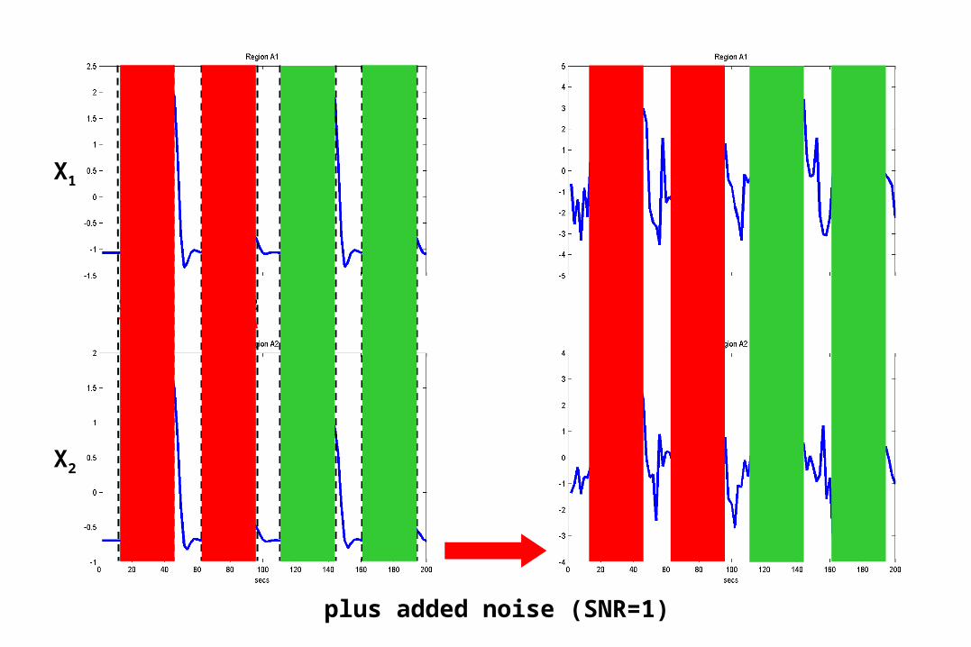
Simulated data

X1

X2

+++X1 X2

Stimulus 2

Stimulus 1

Task A Task B

+++++

++++

– –

Stephan et al. 2007, J. Biosci.

Stim 1Task A

Stim 2Task A

Stim 1Task B

Stim 2Task B

plus added noise (SNR=1)

X1

X2

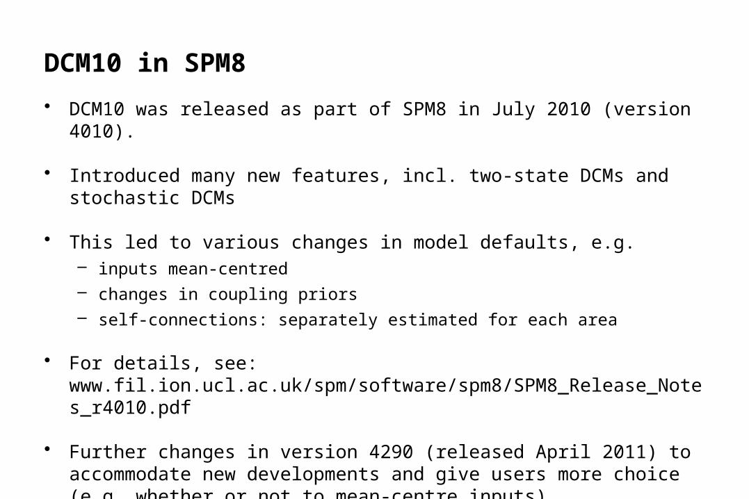
DCM10 in SPM8

• DCM10 was released as part of SPM8 in July 2010 (version 4010).

• Introduced many new features, incl. two-state DCMs and stochastic DCMs

• This led to various changes in model defaults, e.g.– inputs mean-centred– changes in coupling priors– self-connections: separately estimated for each area

• For details, see: www.fil.ion.ucl.ac.uk/spm/software/spm8/SPM8_Release_Notes_r4010.pdf

• Further changes in version 4290 (released April 2011) to accommodate new developments and give users more choice (e.g. whether or not to mean-centre inputs).

The evolution of DCM in SPM

• DCM is not one specific model, but a framework for Bayesian inversion of dynamic system models

• The default implementation in SPM is evolving over time– better numerical routines for inversion– change in priors to cover new variants (e.g., stochastic DCMs,

endogenous DCMs etc.)

To enable replication of your results, you should ideally state which SPM version you are using when publishing papers.

Factorial structure of model specification in DCM10• Three dimensions of model specification:

– bilinear vs. nonlinear

– single-state vs. two-state (per region)

– deterministic vs. stochastic

• Specification via GUI.

bilinear DCM

CuxDxBuAdt

dx m

i

n

j

jj

ii

1 1

)()(CuxBuA

dt

dx m

i

ii

1

)(

Bilinear state equation:

driving input

modulation

driving input

modulation

non-linear DCM

...)0,(),(2

0

uxux

fu

u

fx

x

fxfuxf

dt

dx

Two-dimensional Taylor series (around x0=0, u0=0):

Nonlinear state equation:

...2

)0,(),(2

2

22

0

x

x

fux

ux

fu

u

fx

x

fxfuxf

dt

dx

0 10 20 30 40 50 60 70 80 90 100

0

0.1

0.2

0.3

0.4

0 10 20 30 40 50 60 70 80 90 100

0

0.2

0.4

0.6

0 10 20 30 40 50 60 70 80 90 100

0

0.1

0.2

0.3

Neural population activity

0 10 20 30 40 50 60 70 80 90 100

0

1

2

3

0 10 20 30 40 50 60 70 80 90 100-1

0

1

2

3

4

0 10 20 30 40 50 60 70 80 90 100

0

1

2

3

fMRI signal change (%)

x1 x2

x3

CuxDxBuAdt

dx n

j

jj

m

i

ii

1

)(

1

)(

Nonlinear dynamic causal model (DCM)

Stephan et al. 2008, NeuroImage

u1

u2

V1 V5stim

PPC

attention

motion

-2 -1 0 1 2 3 4 50

0.1

0.2

0.3

0.4

0.5

0.6

0.7

0.8

%1.99)|0( 1,5 yDp PPCVV

1.25

0.13

0.46

0.39

0.26

0.50

0.26

0.10MAP = 1.25

Stephan et al. 2008, NeuroImage

V1

V5PPC

observedfitted

motion &attention

motion &no attention

static dots

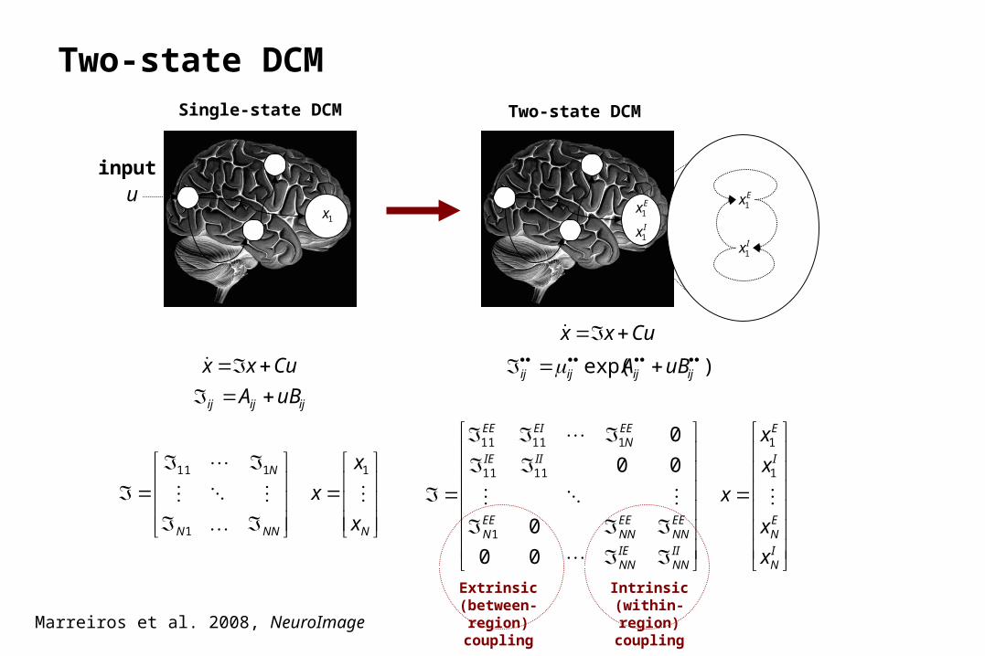
uinput

Single-state DCM

1x

Intrinsic (within-region)

coupling

Extrinsic (between-region)

coupling

NNNN

N

ijijij

x

x

x

uBA

Cuxx

1

1

111

Two-state DCM

Ex1

IN

EN

I

E

IINN

IENN

EENN

EENN

EEN

IIIE

EEN

EIEE

ijijijij

x

x

x

x

x

uBA

Cuxx

1

1

1

1111

11111

00

0

00

0

)exp(

Ix1

I

E

x

x

1

1

Two-state DCM

Marreiros et al. 2008, NeuroImage

0 200 400 600 800 1000 1200-1

-0.5

0

0.5

1inputs or causes - V2

0 200 400 600 800 1000 1200-0.1

-0.05

0

0.05

0.1hidden states - neuronal

0 200 400 600 800 1000 12000.8

0.9

1

1.1

1.2

1.3hidden states - hemodynamic

0 200 400 600 800 1000 1200-3

-2

-1

0

1

2predicted BOLD signal

time (seconds)

excitatorysignal

flowvolumedHb

observedpredicted

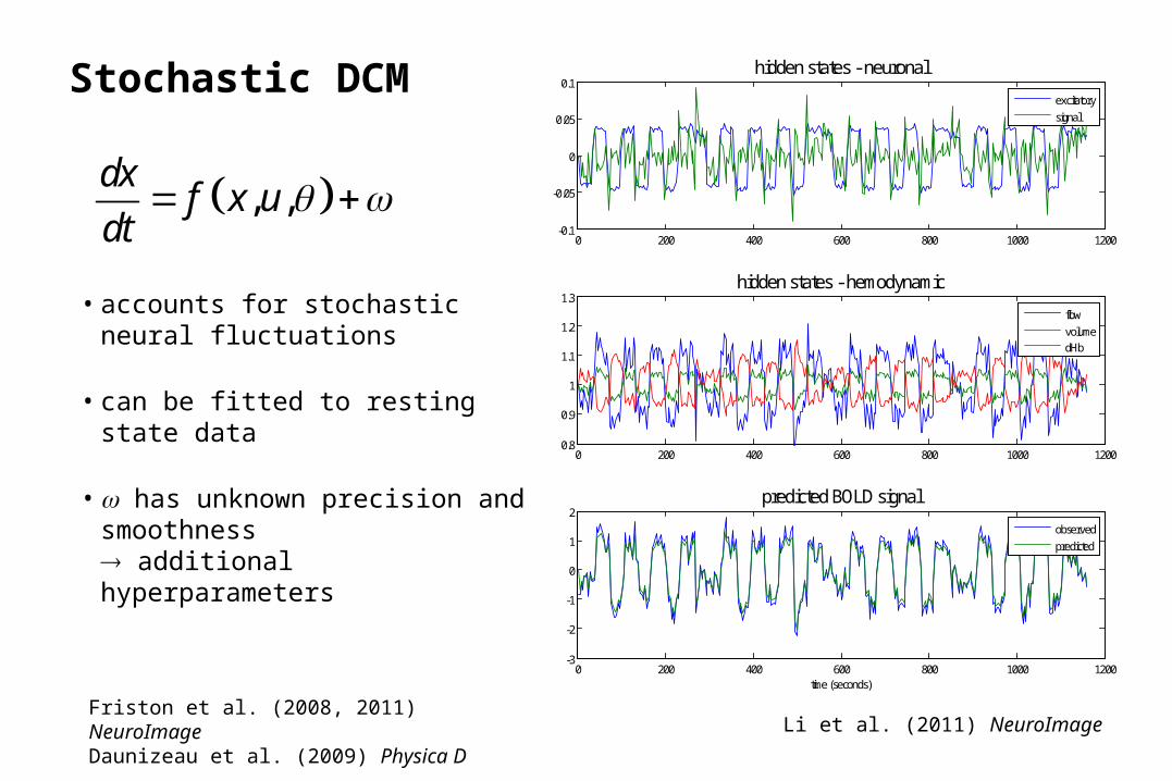
Stochastic DCM

, ,dx

f x udt

Friston et al. (2008, 2011) NeuroImageDaunizeau et al. (2009) Physica D

• accounts for stochastic neural fluctuations

• can be fitted to resting state data

• has unknown precision and smoothness additional hyperparameters

Li et al. (2011) NeuroImage

Thank you