Dynamic data-driven prediction of lean blowout in a … data-driven prediction of lean blowout in a...

Dynamic data-driven prediction of leanblowout in a swirl-stabilized combustor

Soumalya Sarkar†, Asok Ray†, Achintya Mukhopadhyay‡ and Swarnendu Sen‡

†Department of Mechanical & Nuclear Engineering, Pennsylvania State University, University Park, PA 16802, USA

‡Department of Mechanical Engineering, Jadavpur University, Kolkata 700 032, India

(Submission date: June 21, 2014; Revised Submission date: October 29, 2014; Accepted date: December 19, 2014)

ABSTRACTThis paper addresses dynamic data-driven prediction of lean blowout (LBO) phenomena inconfined combustion processes, which are prevalent in many physical applications (e.g., land-based and aircraft gas-turbine engines). The underlying concept is built upon patternclassification and is validated for LBO prediction with time series of chemiluminescence sensordata from a laboratory-scale swirl-stabilized dump combustor. The proposed method of LBOprediction makes use of the theory of symbolic dynamics, where (finite-length) time series dataare partitioned to produce symbol strings that, in turn, generate a special class of probabilisticfinite state automata (PFSA). These PFSA, called D-Markov machines, have a deterministicalgebraic structure and their states are represented by symbol blocks of length D or less, whereD is a positive integer. The D-Markov machines are constructed in two steps: (i) state splitting,i.e., the states are split based on their information contents, and (ii) state merging, i.e., two ormore states (of possibly different lengths) are merged together to form a new state without anysignificant loss of the embedded information. The modeling complexity (e.g., number of states)of a D-Markov machine model is observed to be drastically reduced as the combustorapproaches LBO. An anomaly measure, based on Kullback-Leibler divergence, is constructedto predict the proximity of LBO. The problem of LBO prediction is posed in a patternclassification setting and the underlying algorithms have been tested on experimental data atdifferent extents of fuel-air premixing and fuel/air ratio. It is shown that, over a wide range offuel-air premixing, D-Markov machines with D > 1 perform better as predictors of LBO thanthose with D = 1.

Keywords: Data-driven Dynamics, Lean Blowout, Gas Turbine Combustor, SymbolicDynamics, Probabilistic Finite State Automata

International journal of spray and combustion dynamics · Volume .7 · Number . 3 .2015 – pages 209 – 242 209

*Corresponding author email: [email protected]; [email protected]; [email protected];[email protected]

1. INTRODUCTIONUltra-lean combustion is commonly used for reduction of oxides of nitrogen (NOx) andis susceptible to thermo-acoustic instabilities and lean blowout (LBO). It is well knownthat occurrence of LBO could be detrimental for operations of both land-based andaircraft gas turbine engines. For example, LBO in land-based gas turbines may lead toengine shutdown and subsequent re-ignition involves loss of productivity; similarly,LBO in aircraft gas turbines may cause loss of engine thrust especially if the fuel flowis suddenly reduced during a throttling operation, or if air flow reduction takes place ata much slower rate due to the moment of inertia of the compressor. In essence, a suddendecrease in the equivalence ratio may lead to LBO in gas turbine engines, which couldhave serious consequences. This phenomenon calls for a real-time prediction of LBOand adoption of appropriate measures to mitigate it.

It is noted that a priori determination of the LBO margin may not be feasible,because of flame fluctuations in the presence of thermoacoustic instability. To addressthis issue, the current paper develops an online LBO prediction tool for both well-premixed (e.g., in land-based gas turbines) and partially premixed (e.g., in aircraft gasturbines) combustors. The LBO limit is dependent on a number of parameters that arerelated to the combustor configuration and operating conditions, and monitoring of allthese parameters would require a complicated and expensive diagnostic system. Fromthis perspective, quantifiable dynamic characteristics of flame preceding blowout havebeen exploited in the past as LBO precursors by a number of researchers. De Zilwa et al. [1] investigated the occurrence of blowout in dump combustors with and withoutswirl. Chaudhuri and Cetegen [2], [3] investigated the effects of spatial gradients inmixture composition and velocity oscillations on the blowoff dynamics of a bluff-bodystabilized burner that resembles representative of afterburners of gas turbinecombustors. They used photomultiplier tubes with CH chemiluminescence filters tocapture the optical signal and characterized the signal in the vicinity of blowout.Chaudhuri et al. [4] and Stohr et al. [5] investigated LBO dynamics of premixed andpartially premixed flames using combined particle image velocimetry/planar laser-induced fluorescence (PIV/PLIF)-based diagnostics. However, these works did notfocus on developing strategies for mitigating LBO.

Lieuwen, Seitzman and coworkers [6], [7], [8], [9] used time series data from acousticand optical sensors for early detection and control of LBO in laboratory-scale gas turbinecombustors. Nair and Lieuwen [8] identified blowout parameters using various (e.g.,spectral, statistical, wavelet-based and threshold-based) techniques. For statisticalanalysis, they used moving average kurtosis. They defined thresholds in terms of cut-offsfor peak pressure in a cycle falling below. The number of such events increased sharplynear blowout. For wavelet-based analysis, they used the Mexican Hat and a customizedwavelet that matches with the time series data of OH* chemiluminescence. Yi andGutmark [10] identified two indices, namely, normalized chemiluminescence root meansquare and normalized cumulative duration of LBO precursor events, for LBO predictionin real time. However, both Lieuwen et al. and Gutmark demonstrated their techniques forLBO prediction in premixed combustors. On the other hand, Mukhopadhyay and co-workers [11], [12] developed a number of techniques for early detection of LBO, which

210 Dynamic data-driven prediction of lean blowout in a swirl-stabilized combustor

worked satisfactorily over a wide range of fuel-air premixing. Chaudhari et al. [11] usedflame color to device a novel and inexpensive strategy for LBO detection. In this work,they used as an LBO detection metric, the ratio of red and blue intensities in the flameimage obtained with a commercial color charge-coupled device (CCD) camera.Mukhopadhyay et al. [12] used chemiluminescence time series data for online predictionof LBO under both premixed and partially premixed operating conditions. The algorithmwas built upon a data-driven symbolic-dynamics-based technique, called D-Markovmachine [13], [14], where the parameter D was set to 1 to construct the probabilistic finitestate automata (PFSA), which implies that the memory of the underlying combustionprocess was restricted only to its immediate past state.

In a number of recent publications, the transition to LBO was correlated withchanges in signature of the dynamic characteristics of the system. Kabiraj et al. [15] andKabiraj and Sujith [16] investigated dynamics of a ducted laminar premixed flame andusing tools of dynamical systems analysis demonstrated that the system undergoes anumber of bifurcations involving quasiperiodic and intermittent behaviors leading toblowout. Gotoda and co-workers [17] used a number of analytical tools to examine thedynamics of a model gas turbine combustor and showed that close to lean blowout thedynamics of the combustor exhibits a self-affine structure indicating fractionalBrownian motion but changes to chaotic oscillations showing oscillations with slowamplitude modulation as the equivalence ratio increases. Gotoda et al. [18] showed thatthe relatively regular pressure oscillations undergo transition to intermittent chaoticoscillations as the equivalence ratio is decreased and the system approaches LBO.Translational errors were used to measure the parallelism of neighboring trajectories inthe phase space as a control variable for mitigation of LBO. Through similar studies,Sujith and co-workers [19], showed that combustion noise is due to chaotic fluctuationsof moderately high dimension that undergoes transition to high amplitude oscillationscharacterized by periodic behavior. This information was used to determine the loss ofchaos in the system dynamics as a precursor for prediction of thermoacoustic instability.

The current paper is a major extension of the earlier work on D-Markov machine-based LBO prediction, reported by Mukhopadhyay et al. [12]. The significantcontributions of the current paper in the context of dynamic data-driven applicationsystems (DDDAS) [20] are delineated below.

1) State splitting and state merging: The states of the D-Markov machine areconstructed in two steps [14]: (i) state splitting, i.e., the states are split basedon their information contents, and (ii) state merging, i.e., two or more states(of possibly different lengths) are merged together to form a new state withoutany significant loss of their embedded information.

2) Accommodation of a longer memory of chemiluminescence time series:Algorithms of the D-Markov machine are reformulated with D > 1 (instead ofD = 1) to extract low-dimensional features with a longer history of thecombustion process.

3) Bias removal to achieve leaner operating conditions: The bias (i.e., the non-zero mean) is removed from chemiluminescence time series to avoid mean-based prediction that may result in richer operating conditions with consequentpenalties of enhanced NOx emission.

International journal of spray and combustion dynamics · Volume .7 · Number . 3 . 2015 211

4) Information-theoretic anomaly measure for LBO prediction: An anomalymeasure [13] is constructed, based on Kullback- Leibler divergence [21], toanticipate the proximity of LBO with increased sensitivity.

5) Pattern classification based on the features extracted from chemiluminescencetime series: The prediction of LBO is posed as a pattern classification problembased on different ranges of the equivalence ratio at several premixing levels.This approach largely alleviates the problem of loss of robustness due tolimited data availability for making online decisions [22].

The paper is organized in five sections, including the present one, and threeappendices. Section 2 describes a laboratory- scale swirl-stabilized dump combustor,which has been used for prediction of LBO phenomena from time series of opticalsensor data. Section 3 explains the method of information extraction from time seriesas a D-Markov machine in the form of low-dimensional features. Section 4 presents thecapability and advantages of the proposed approach for LBO prediction over differentparameter ranges. Finally, the paper is summarized and concluded in Section 5 withselected recommendations for future research. Appendix A explains the notion of two-time-scale behavior of combustion dynamics, which are captured from the sensor timeseries data. Appendix B explains in detail the key mathematical concepts that arenecessary for construction of the pattern classification algorithms in the context of D-Markov machines. Appendix C lists the four algorithms of state splitting and statemerging in the construction of D-Markov machines, from which the computer codescan be readily developed.

2. APPARATUS FOR EXPERIMENTAL RESEARCHA swirl-stabilized dump combustor, as depicted in Figure 1, was designed as alaboratory-scale model of a generic gas turbine combustor based on the earlier worksof Williams et al. [24], Meier et al. [25], Nair et al. [6], Chaudhuri and Cetegen [2] andYi and Gutmark [10]. The air is supplied at the ambient temperature from a compressorto the bottom port on the premixing tube and the air flow rate is measured upstream ofthe combustor by using a calibrated mass flow controller (MFC) (Aalborg range 0 to500 litres per minute (lpm)). Liquefied petroleum gas (LPG), having a composition of40% propane (C3H8) and 60% butane (C4H10) by volume, has been used as the fuel inthe experiments. The fuel is supplied from a pressurized cylinder fitted with needlevalve to control the flow rate and is also measured upstream of the combustor by acalibrated Aalborg mass flow controller (Range: 0 – 10 lpm). To investigate the effectsof premixing on flame dynamics, six side ports are provided 50 mm apart along thelength of the premixing tube, as seen in Figure 1. This arrangement allows the fuel tobe injected at different axial positions of the premixing tube, thereby providing differentpremixing lengths. The ports are numbered 1 to 6 from the bottom of the premixingtube. Thus the fuel injected through Port 1 allows greatest premixing while Port 6allows least premixing. The fuel is injected to one of the side ports of the premixingtube. The fuel-air mixture enters the combustor through the inlet swirler in the annulusaround a center body, located just prior to the dump plane in the premixing section. Theinner diameter of the premixing section is 23 mm, and the diameter of the center-body


is 8 mm. The inlet swirler has six vanes positioned at 60o to the flow axis. A quartz tubeis provided in the combustion zone having the internal diameter 60 mm and length 200mm to facilitate optical diagnostics.

The heat release rate is measured by the chemiluminescence emitted from the CH*radicals (wavelength λ 431 nm) of the flame. The time series data are obtained witha photomultiplier tube (PMT) fitted with an optical band pass filter (λpass = 430 nm)with full-width at half-maximum (FWHM) =10 nm. The PMT output signal (in volts)is acquired using a 16-bit analog input channel on a National Instruments P X I-6250data acquisition card that is mounted in a National Instruments P X I-1050 Chassis


Photo multiplertube (PMT)

Fuel inlet

1

2

3

4

5

6

Flame

Air inlet

L =

200

mm

L =

350

mm

Pre

mix

ing

tube

Fue

l por

ts

Mas

s flo

w c

ontr

olle

r (M

FC

)

Dat

a ac

quis

ition

sys

tem

(Sig

nal c

ondi

tione

r, N

I PX

I, pC

)

Sw

irler

CombustorQuartz tubeInt Dia = mm

Figure 1: Schematic View of the Laboratory Apparatus.

having a built-in 08 channel S C X I -1125 signal conditioner module. Time series datawith 215 points have been acquired at a sampling frequency of 2 kHz in eachexperiment. Video images of the flame are recorded in order to visualize LBOphenomenology and correlate the same with the optical signal. Still color images of theflame are also acquired simultaneously using the digital single lens reflex (DSLR)camera at suitable exposure to avoid pixel saturation. Further details of theexperimental apparatus and instrumentation are available in [23].

Experiments were carried out using liquefied petroleum gas (LPG) as the fuel. A major reason for the choice of LPG as the fuel is that LPG consists of mainly propaneand butane, which are the simplest hydrocarbons whose combustion exhibits thechemical behavior, flame speed, and extinction limits closer to the heavier and morecomplex hydrocarbon fuels [26]. Tests were first conducted with stoichiometric fuel/airmixture (i.e., φ = 1). Then, at each given air flow rate, the fuel supply was graduallydecreased to generate progressively lean reacting mixtures. A constant air flow rate inthe experiments was maintained to ensure that the Reynolds number of fluid flowremains practically constant because air constitutes the bulk of the incoming reactantmixture.

3. LBO PREDICTION VIA SYMBOLIC ANALYSISSymbolic time series analysis (STSA) [27] is built upon the concept of symbolicdynamics [28] that deals with discretization of dynamical systems in both space and time.The notion of STSA has led to the development of a feature extraction tool for patternclassification, in which a time series of sensor signals is represented as a symbol sequencethat, in turn, leads to the construction of probabilistic finite state automata (PFSA)[29][30]. Statistical patterns of slowly evolving dynamical behavior in physical processescan be identified from sensor time series data and often the changes in these statisticalpatterns occur over a slow time scale with respect to the fast time scale of processdynamics. The concept of two time scales is succinctly presented in Appendix A.

Since PFSA models are capable of efficiently compressing the informationembedded in sensor time series [13][31], these models could enhance the performanceand execution speed of information fusion and information source localization that areoften computation-intensive. Rao et al. [32] and Bahrampour et al. [33] have shownthat the performance of this PFSA-based tool as a feature extractor for statistical patternrecognition is comparable (and often superior) to that of other existing techniques (e.g.,Bayesian filters, Artificial Neural Networks, and Principal Component Analysis [34]).Mathematical preliminaries and background information on symbolic dynamics arepresented in Appendix B.

The major steps for construction of PFSA from sensor signal outputs (e.g., timeseries) of a dynamical system are as follows.

1) Coarse-graining of time series to convert the scalar or vector-valued data intosymbol strings, where the symbols are drawn from a (finite) alphabet [35].

2) Encoding (i.e., identification of labeled graph structure and pertinentparameters) of probabilistic state machines from the symbol strings [13], [14],[31], [22], [36].


The next step is to construct probabilistic finite state automata (PFSA) from thesymbol strings to encode the embedded statistical information so that the dynamicalsystem’s behavior is captured by the patterns generated from the PFSA in a compactform. The algebraic structure of PFSA (i.e., the underlying FSA) consists of a finite setof states that are interconnected by transitions [37], where each transition correspondsto a symbol in the (finite) alphabet. At each step, the automaton moves from one stateto another (including self loops) via these transitions, and thus generates acorresponding block of symbols so that the probability distributions over the set of allpossible strings defined over the alphabet are represented in the space of PFSA. Theadvantage of such a representation is that the PFSA structure is simple enough to beencoded as it is characterized by the set of states, the transitions (i.e., exactly onetransition for each symbol generated at a state), and the transition’s probability ofoccurrence.

D-Markov machines are models of probabilistic languages where the future symbolis causally dependent on the (most recently generated) finite set of (at most) D symbolsand form a proper subclass of PFSA with applications in various fields of research suchas anomaly detection [13] and robot motion classification [38]. The underlying FSA inthe PFSA of D-Markov machines are deterministic, i.e., the future state is adeterministic function of the current state and the observed symbol. Therefore, D-Markov machines essentially encode two entities: (1) probability of generating asymbol at a given state, and (2) deterministic evolution of future states from the currentstate and the symbol. It is noted that if the symbol is not observed, the description ofthe state transition in the D-Markov machine becomes a probabilistic Markov chain.Furthermore, under the assumption of irreducibility, the statistically stationarydistribution of states is unique and can be computed. This class of PFSA (i.e., D-Markov machines) is a proper subclass of probabilistic non-deterministic finite stateautomata which is equivalent to Hidden Markov Models (HMMs) [29]. Even thoughHMMs form a more general class of models, the deterministic properties of D-Markovmachines present significant computational advantages. For example, due to theconstrained algebraic structure of D-Markov machines, it is possible to constructalgorithms for efficient implementation and learning.

Since long-range dependencies in the time series rapidly diminish under theassumption of strong mixing [39], such a dynamical system could be modeled as a D-Markov machine with a sufficiently large value of D. However, increasing the valueof D may lead to an exponential growth in the number of machine states and hence thecomputational complexity of the model grows. The main issue addressed in this paperis order reduction of the states of a D-Markov machine model for representing thestationary probability distribution of the symbol strings that are generated from thetimes series of a dynamical system [14]. In addition, this paper addresses the trade-offbetween modeling accuracy and model order, represented by the number of states, forthe proposed algorithm. The power of the proposed tool of PFSA-based D-Markovmachines is its capability of real-time execution on in-situ platforms for anomalydetection, pattern classification, condition monitoring, and control of diverse physicalapplications.


A. Construction of D-Markov MachinesThis subsection develops the pertinent concepts that are necessary to construct a

D-Markov machine. The PFSA model of the D-Markov machine generates symbolstrings on the underlying Markov process. The generation

of a symbol depends only on the current state in the PFSA structure of a D-Markovmachine. However, if the state is unknown, the next symbol generation may depend onthe history of the symbol generated by the PFSA. In the PFSA model, a transition fromone state to another is independent of the previous states. Therefore, the states andtransitions form a Markov process, which is a special class of Hidden Markov Models(HMM) [30]. However, from the perspectives of PFSA construction from a symbolsequence, the states are implicit and generation of the next symbol may depend on thecomplete history of the symbol sequence. In the construction of a D-Markov machine[13], generation of the next symbol depends only on a finite history of at most Dconsecutive symbols, i.e., a symbol block of length not exceeding D. A formaldefinition of the D-Markov machine follows.

Definition 3.1 (D-Markov Machine [13]) A D-Markov machine is a PFSA (seeDefinition B.5 in Appendix B) and it generates symbols that solely depend on the (mostrecent) history of at most D symbols in the sequence, where the positive integer D iscalled the depth of the machine. Equivalently, a D-Markov machine is a statisticallystationary stochastic process S = s-1s0s1 , where the probability of occurrence ofa new symbol depends only on the last D symbols, i.e.,

(1)

Consequently, for w D (see Definition B.2), the equivalence class *w of all(finite-length) words, whose suffix is w, is qualified to be a D-Markov state that isdenoted as w.

Considering the set of all symbol blocks of length D as the set of states, one mayconstruct a D-Markov machine from a symbol sequence by frequency counting toestimate the probabilities of each transition. Since the number of states increasesexponentially as the depth D is increased, state merging might be necessary for orderreduction of D-Markov machines with relatively large values of D.

Given a finite-length symbol sequence S over a (finite) alphabet , there existseveral PFSA construction algorithms to discover the underlying irreducible PFSAmodel K of S, such as causal-state splitting reconstruction (CSSR) [36] and D-Markov[13], [14]. All these algorithms start with identifying the structure of the PFSA K � (Q,, δ, π) (see Appendix B). Then, to estimate the morph matrix, a |Q| || countmatrix C is initialized to the matrix, each of whose elements is equal to 1.

Let Nij denote the number of times that a σj is generated from the state qi uponobserving the sequence S. An estimate of the probability map for the PFSA K iscomputed by frequency counting as

(2)

N� �� ∈ ∀ ∈Σs s s s{ : , }1 2

� � �⎡⎣⎢

⎤⎦⎥ =

⎡⎣⎢

⎤⎦⎥− − − −P s s s P s s sn n D n n n D n1 1

�� ∑ ∑

π σ =+

Σ +q

C

C

N

Nˆ( , )

1

| |i jij

i

ij

i


The rationale for initializing each element of the count matrix C to 1 is that if noevent is generated at a state q Q, then there should be no preference to any particular

symbol and it is logical to have i.e., the uniform distribution of

event generation at the state q. The above procedure guarantees that the PFSA,constructed from a (finite-length) symbol string, must have an (elementwise) strictlypositive morph map P, as stated in Definition B.6 of Appendix B.

B. Algorithm DevelopmentThis subsection develops the algorithms for construction of D-Markov machines. Theunderlying procedure consists of two major steps, namely, state splitting and statemerging. In general, state splitting increases the number of states to achieve moreprecision in representing the information content in the time series. This is performedby splitting the states that effectively reduce the entropy rate H(|Q), thereby focusingon the critical states (i.e., those states that carry more information). Although thisprocess is executed by controlling the exponential growth of states with increasingdepth D, the D-Markov machine still may have a large number of states. Thesubsequent process reduces the number of states in the D-Markov machine by mergingthose states that have similar statistical behavior. Thus, a combination of state splittingand state merging, described in Algorithms 1, 2, 3 and 4 in Appendix C leads to the finalform of the D-Markov machine.

1) The State Splitting Algorithm: In D-Markov machines, a symbol block of (finite)length D is sufficient to describe the current state. In other words, the symbols thatoccur prior to the last D symbols do not affect the subsequent symbols observed.Therefore, the number of states of a D-Markov machine of depth D is bounded aboveby ||D , where || is the cardinality of the alphabet . For example, with the alphabetsize || = 4 (i.e., 4 symbols in the alphabet ) and a depth D = 3, the D-Markovmachine could have at most ||D = 64 states. As this relation is exponential in nature,the number of states rapidly increases as D is increased. However, form the perspectiveof modeling a symbol string, some states may be more important than others in termsof their embedded information contents. Therefore, it is advantageous to have a set ofstates that correspond to symbol blocks of different lengths. This is accomplished bystarting off with the simplest set of states (i.e., Q = for D = 1) and subsequentlysplitting the current state that results in the largest decrease of the entropy rate.

The process of splitting a state q Q is executed by replacing the symbol block q byits branches as described by the set {σq : σ } of words. Maximum reduction of theentropy rate is the governing criterion for selecting the state to split. In addition, thegenerated set of states must satisfy the self-consistency criterion, which only permits aunique transition to emanate from a state for a given symbol. If δ(q, σ) is not unique foreach σ , then the state q is split further. In the state splitting algorithm, a stoppingrule is constructed by specifying the threshold parameter ηspl on the rate of decrease ofconditional entropy. An alternative stopping rule for the algorithm is to provide amaximal number of states Nmax instead of the threshold parameter ηspl. The operationof state splitting is described in Algorithm 1 (see Appendix C).

π σ σ=Σ∀ ∈Σqˆ( , )

1| |

,


Let q be a D-Markov state (see Definition 3.1), which is split to yield new states σq,where σ and σq represents the equivalence class of all (finite-length) symbolstrings with the word σq as the suffix. Figure 2 illustrates the process of state splittingin a PFSA with alphabet = {0, 1}, where each terminal state is circumscribed by anellipse. For example, the states in the third layer from the top are: 00q, 10q, 01q, and11q, of which all but 10q are terminal states. Consequently, the state 10q is further splitas 010q and 110q that are also terminal states, i.e, Q = {00q, 01q, 11q, 010q, 110q},as seen in the split PFSA diagram of Figure 2. Given the alphabet and the associatedset Q of states, the morph matrix P can be computed in the following way.

(3)

where P() and P(|) are the same as those used in Definition B.7 and Eq. (14) therein.For construction of PFSA, each element p(σ, q) of the morph matrix P is estimated

by frequency counting as the ratio of the number of times, N(qσ), the state q is followed(i.e., suffixed) by the symbol σ and the number of times, N(q), the state q occurs. Byusing the structure of Eq. (2), it follows from Eq. (3) that each element p̂(σ, q) of theestimated morph matrix P̂ is obtained as

(4)

where

Similar to Eq. (4) and following the structures of Eq. (2), each element P(q) of thestationary state probability vector is estimated by frequency counting as

(5)

π σ σσ

σ= = ∀ ∈Σ∀ ∈q P qP qP q

q Q( , ) ( | )( )( )

�π σσ

σ+Σ +

∀ ∈Σ∀ ∈qN q

N qq Qˆ( , )

1 ( )| | ( )

∑ π σ = ∀ ∈σ∈Σ

q q Qˆ( , ) 1 .

��∑++ ′

∀ ∈

′∈

P qN q

Q N qq Q( )

1 ( )| | ( )

q Q


q

0q00q

00q 10q

010q 110q

1q

01q 11q

Figure 2: Tree-representation of state splitting in D-Markov machines.

where is an element of the estimated stationary state probability vector, which

implies the estimated stationary probability of the PFSA being in the state q Q. Wenet al. [22] have statistically modeled the error of estimating the state probability vectorfrom finite-length symbol strings.

Now the entropy rate (see Eq. (14) in Appendix B) is computed in terms of theelements of estimated state probability vector and estimated morph matrix as

(6)

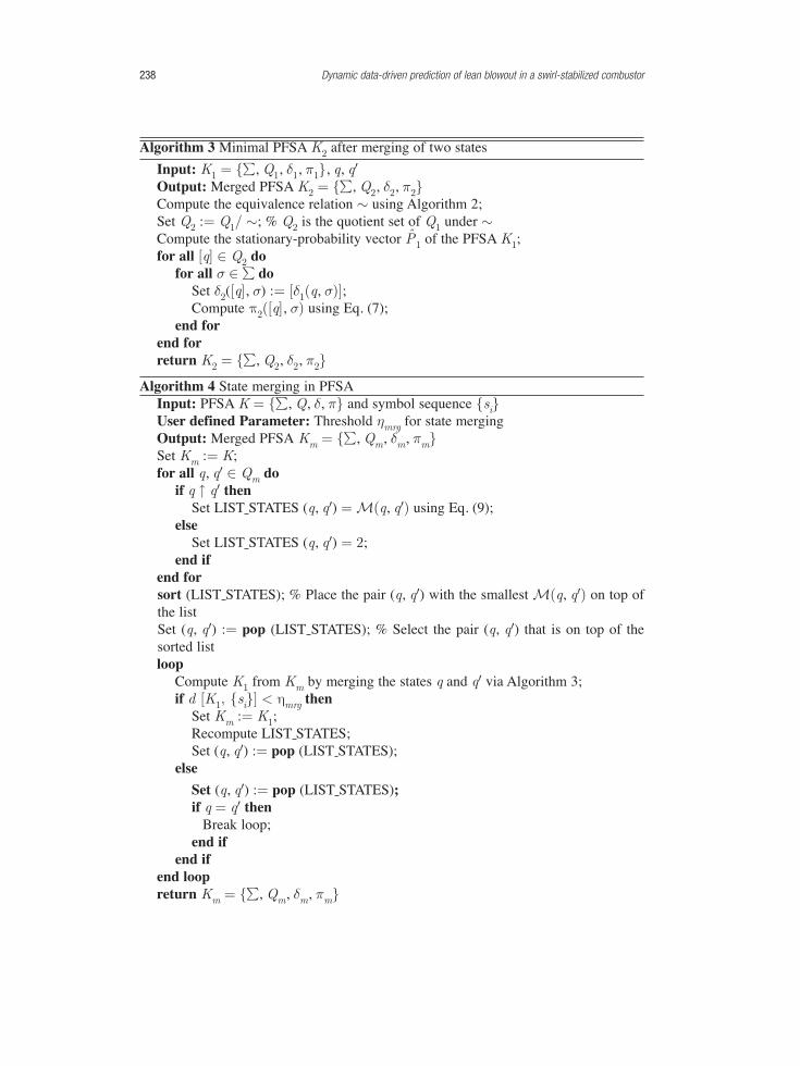
2) The State Merging Algorithm: Once state splitting is performed, the resulting D-Markov machine is a statistical representation of the symbol string underconsideration. Depending on the choice of alphabet size || and depth D, the numberof states after splitting may run into hundreds. Although increasing the number of statesof the machine may lead to a better representation of the symbol string, it rapidlyincreases the execution time and memory requirements. The motivation behind the statemerging is to reduce the number of states, while preserving the D-Markov structure ofthe PFSA. Of course, such a process may cause the PFSA to have degraded precisiondue to loss of information. The state merging algorithm aims to mitigate this risk.

In the state merging algorithm, a stopping rule is constructed by specifying anacceptable threshold ηmrg on the distance F(, ) between the merged PFSA and thePFSA generated from the original time series. Before embarking on the state mergingalgorithm, the procedure for merging of two states is described below.

Notion of merging two states: The process of state merging is addressed by creatingan equivalence relation [40], denoted as , between the states. The equivalence relationspecifies which states are identified to belong to the same class, thereby partitioning theoriginal set of states into a smaller number of equivalence classes of states, each beinga nonempty collection of the original states. The new states are, in fact, equivalenceclasses as defined by .

Let K1 = {, Q1, δ1, π1} be the split PFSA, and let q, q Q1 be two states that areto be merged together. Initially, an equivalence relation is constructed, where none ofthe states are equivalent to any other state except itself, i.e., each equivalence class isrepresented by a singleton set. To proceed with the merging of states q and q, anequivalence relation is imposed between q and q, denoted as q q; however, thetransitions between original states may not be well-defined anymore, in the followingsense: there may exist σ such that the states δ1(q, σ) and δ2(q, σ) are not equivalent.In essence, the same symbol may cause a transition to two different states from themerged state {q, q}. As the structure of D-Markov machines does not permit thisambiguity of non-determinism [13], the states δ1(q, σ) and δ2(q, σ) are also required tobe merged together, i.e., δ1(q, σ) δ2(q, σ) (this procedure is known as determinizationin the state merging literature). Therefore, the symbol σ will cause a transition from themerged state {q, q} to the merged state {δ1(q, σ), δ2(q, σ)}. This process is recursive

�

∑∑

∑∑

σ σ

π σ π σ

Σ =−

≈−

σ

σ

∈Σ∈

∈Σ∈

H Q P q P q P q

P q q q

( | ) ( ) ( | ) log ( | )

( )ˆ( , ) log ˆ( , )

q Q

q Q

�P q( )


and is performed until no ambiguity in state transitions occurs. Indeed at each iteration,the number of states of the future machine is reduced, and the machine where all thestates are merged is always consistent. Therefore, the number of states is a decreasingsequence of positive integers, which must eventually converge. The recursive operationof the equivalence relation is described in Algorithm 2 (see Appendix C).

Let K1 = {, Q1, δ1, π1} be the split PFSA that is merged to yield the reduced-orderPFSA K2 = {, Q2, δ2, π2}, where the state-transition map δ2 and the morph function π2for the merged PFSA K2 are defined on the quotient set Q2 � Q1/, and [q] Q2 is theequivalence class of q Q1. Then, the associated morph function p2 is obtained as:

(7)

As seen in Eq. (7), the morph function π2 of the merged PFSA K2 is estimated as thesum of p̂1 weighted by the stationary state probabilities of the PFSA K1. Byconstruction, δ2 is naturally obtained as

(8)

Algorithm 3 in Appendix C presents the procedure to obtain the PFSA, where theobjective is to merge the states q and q.

Identification of the states to be merged: The next task is to decide which states haveto be merged. States that behave similarly (i.e., have similar morph probabilities) havea higher priority for merging. The similarity of two states, q, q Q, is measured interms of morph functions (i.e., conditional probabilities) of future symbol generation asthe distance between the two rows of the estimated morph matrix P̂ corresponding tothe states q and q. The �1-norm (i.e., the sum of absolute values of the vectorcomponents) has been adopted to be the distance function as seen below.

(9)

∪ �

�

�

�

�

�

∑

∑

π σ σ

σ

= = =⎡

⎣⎢⎢

⎤

⎦⎥⎥

== =

=

+∈

∈+

∈

q P s X q

P s X q

P X q

([ ], ) | { }

[ ;{ }]

( )

i iq q

q qi i

q qi

2 1[ ]

[ ]1

[ ]

� �

�

�

�

�

�

�

�

�

�

∑

∑

∑

∑

σ

π σ

== = =

=

≈×

∈+

∈

∈

∈

P s X q P X q

P X q

q P q

P q

[ | ] ( )

( )

ˆ ( , ) ( )

( )

q qi i i

q qi

q q

q q

[ ]1

[ ]

1[ ]

1

1

[ ]

�P1

δ σ δ σ=q q([ ], ) [ ( , )]2 1

M � �

∑π π

π σ π σ

′ ⋅ − ′ ⋅

= − ′σ∈Σ

q q q q

q q

( , ) || ˆ( , ) ˆ( , ) ||

| ˆ( , ) ˆ( , ) |1


A small value of M(q, q) indicates that the two states have close probabilities ofgenerating each symbol. Note that this measure is bounded above as M(q, q) 2 q,q Q, because and Now the procedure of

state merging is briefly described below.First, the two closest states (i.e., the pair of states q, q Q having the smallest value

of M(q, q)) are merged using Algorithm 3 (see Appendix C). Subsequently, distanceF(, ) (see Eq. (15) in Subsection B-C) of the merged PFSA from the initial symbolstring is evaluated. If F < ηmrg where ηmrg is a specified threshold, then the machinestructure is retained and the states next on the priority list are merged. On the otherhand, if F ≥ ηmrg, then the process of merging the given pair of states is aborted andanother pair of states with the next smallest value of M(q, q) is selected for merging.This procedure is terminated if no such pair of states exist, for which F < ηmrg. Theoperation of the procedure is described in Algorithm 4 (see Appendix C).

3) Feature Extraction: After the D-Markov machine is constructed, the stationarystate probability vector is computed in the following way. Similar to Eq. (4), eachelement of the stationary state probability vector P(q) is estimated by frequencycounting as (see Eq. (5)).

The estimated stationary state probability vector serves as a feature vectorrepresenting the associated time series for classification of different zones of flame; thisfeature vector is low-dimensional and can be computed in real time, based on thevarying equivalence ratio before the onset of LBO. For example, if the alphabet is {1,2, 3, 4, 5}, the set of states after state splitting is {1, 2, 13, 23, 33, 43, 53, 14, 24, 34,44, 54, 5} for port 3 and state merging leads to the set of states, {1, 2, 13, 23, 33, 43,53, {14, 24, 34}, 44, 54, 5}. The stationary state probability vector computed from theD-Markov machine with proposed state description, served as the feature for thisprediction problem. Figure 3 shows the state probability vectors fromchemiluminescence time series at three different stages of fuel-air ratios.

∑ π≤ ′ ⋅ ≤σ∈Σ

q0 ˆ( , ) 1.∑ π≤ ⋅ ≤σ∈Σ

q0 ˆ( , ) 1

�P q( )�P q( )


0.3

0.2

0.1

01 2 3 4 5 6 7 8

State index

9 1011

Pro

babi

lity

111 2 3 4 5 6 7 8

State index

9 10

0.3

0.2

0.1

0

Pro

babi

lity

1 2 3 4 5 6 7 8

State index

9 1011

0.3

0.2

0.1

0

Pro

babi

lity

3210

CH

* In

tens

ity (

a.u.

)

0 1

Data sequence

× 104 × 104 × 104

2 3

-1

Data sequence

0 1 2 3

3210

CH

* In

tens

ity (

a.u.

)

-1

Data sequence

0 1 2 3

3210

CH

* In

tens

ity (

a.u.

)

-1

Figure 3: Markov machine features from chemiluminescence time-series for threedifferent stages of fuel-air ratios (from left to right: φ = 0.90, φ = 0.74and φ = 0.66) for airflow at 150 lpm for Lfuel = 250 mm (Port 3).

4) Kullback-Leibler Divergence as LBO measure: Let be the estimated stateprobability vector (see Eq. (5)) of the resulting probabilistic finite state automaton(PFSA) model at the reference epoch τ0 in the slow time scale (see Appendix A) and let

be the estimated state probability vector of the (possibly evolved) PFSA model atan epoch tk . Relative to the reference flame condition at the epoch τ0, any anomalous

behavior of the current flame condition at the epoch τk is expressed in terms of and

as the (scalar) Kullback-Leibler divergence [21] that is defined as

(10)

where other choices of the divergence (e.g., standard Euclidean distance) can also bemade (for example, see [13]). A special advantage of using the Kullback-Leiblerdivergence is that it provides an average anomaly measure of the current the flamerelative to the reference condition in the log scale. It is noted that, in Eq. (10), the

standard conventions 0 log(0) = 0 and are applicable based on

the continuity arguments. However, such a singularity condition is highly undesirablefor continous monitoring and control of flame stability and it is avoided by appropriateselection of the reference vector , each of whose elements is strictly positive.

5) Pattern Classification: The next step is classification of patterns among the featuresextracted from the time series data. A nested classification architecture, as shown in Figure4, is proposed based on the range of the non-dimensional ratio of φ/φLBO to predict a

��

�∑⎛

⎝

⎜⎜⎜⎜⎜

⎞

⎠

⎟⎟⎟⎟⎟⎟∈

d P P P qP q

P q( || ) ( ) log

( )

( )

k k

q Q

k0

0

�Pk

�P0

�Pk

⎛⎝⎜⎜⎜⎞⎠⎟⎟⎟=∞∀ ∈ ∞p

pplog

0(0, )

�P0

�P0


Chemiluminescence time-series

AlarmNominalφ / φLBO > 1.2

Progressive LBO1.1 < φ/φLBO ≤ 1.2

Impending LBO1 ≤ φ/φLBO ≤ 1.1

Figure 4: Nested classification for lean blowout (LBO) prediction.

forthcoming LBO, irrespective of the airflow rates for a certain premixing level. Initially,the chemiluminescence time series of duration 16 sec for different premixing lengths weregrouped into two classes as: Alarm (1 φ/φLBO 1.20) and Nominal (φ/φLBO > 1.20).The class Alarm was divided into two finer classes as: Impending LBO (ILBO) for 1 φ/φLBO 1.1, and Progressive LBO (PLBO) for 1.1 < φ/φLBO 1.2. Identification ofthe PLBO phase is crucial for LBO mitigation as the control actions need to be initiatedtypically near the PLBO-ILBO boundary.

While there are many tools for pattern classification [34], this paper makes uses oftwo well known techniques, namely, leave-one-out and support vector machines (SVM).The leave-one-out method is adopted, because of the limited availability of training and test data; it makes use of the cross validation concept, where n groups of (n - 1)training data are used with the remaining one of the n available measurements beingtreated as test data. In Section 4, the SVM method with either a Gaussian or a linearkernel [34] has been used to determine the classes to which the test features belong.

4. RESULTS AND DISCUSSIONSThis section validates the algorithms of D-Markov machines for LBO prediction on theensemble of time series data that were generated from the swirl-stabilized dumpcombustor described in Section 2. Multiple experiments have been conducted withliquefied petroleum gas (LPG) fuel at airflow rates of 150, 175 and 200 lpm for threedifferent fuel-air premixing lengths (i.e., distance of fuel injection port from the dumpplane) of Lfuel = 350 mm, 250 mm, and 150 mm for Port 1, Port 3, and Port 5,respectively, where Reynolds numbers based on cold flow conditions have been up to18, 700 at 200 lpm.

A. Experimental ObservationsThe combustion process was relatively steady and occupied the whole combustor whilethe shape of the flame was conical as the fuel was injected through Port 1 (with Lfuel =350 mm) at stoichiometric air-fuel mixture (i.e., φ = 1) . As the equivalence ratio wasreduced to φ = 0.81 case, there was a significant change in the flame color; it becamebluish with a reddish tip while retaining a well defined combustion region. Forconditions close to LBO (e.g., φ = 0.75) the flame shape changed from conical toelongated columnar due to reduced reaction rate and burning velocity of flame nearLBO. There were random instances of flame oscillations and flame lift-off from thedump plane. As the unburned fuel was reignited, the flame became detached from thecenter body and returned to the inlet. The random occurrences of unique extinction andre-ignition events spanned a period of several milliseconds prior to LBO.

The observations with the minimum premixing length Lfuel = 150 mm weresignificantly different from those of larger premixing lengths for operations near theLBO limit. The flame was attached to the dump plane and did not show any lift-offpattern at all times due to lower fuel-air premixing. The flame intensity wassignificantly reduced and, after a subsequent reignition, the flame did not oscillate andthe precursor events were not so intense. Furthermore, the flame was not symmetricallyattached to the dump plane and exhibited asymmetric spread with a flickering nature.


B. Reduction of Modeling Complexity near Lean BlowoutEach chemiluminescence time-series is converted to zero mean by subtracting the biaswhich is a dominating factor in generating the anomaly measure in the symbolicanalysis, reported by Mukhopadhyay et al. [12]. The removal of the bias has yielded asignificant improvement in the performance of LBO prediction over the previousstrategy [12], because mean-based detection may lead to the controller operating theengine at relatively richer conditions with consequent penalties of enhanced NOxemission. Since there is no bias in the algorithms reported in this paper, the texture oftime series data is modeled precisely to predict LBO ahead of time. The reference timeseries (i.e., at φ = 1) for different premixing lengths are partitioned for an alphabet sizeof seven (i.e., || = 7) via maximum entropy partitioning (MEP) [14], [31]. Thisinformation on partitioning has been used to symbolize the data set at differentequivalence ratios (i.e., for φ < 1) for the corresponding premixing length. Once thetime series data are symbolized, D-Markov machines are constructed from the symbolstrings via state splitting and state merging.

Figure 5 shows that the number of states of the D-Markov machine after statesplitting and state merging reduces approximately monotonically as the equivalenceratio is dropped for Lfuel = 350) mm. In this case, state splitting is done with an upperbound of 30 PFSA states (i.e., Nmax = 30 in Algorithm 1 of Appendix C) and statemerging with a threshold parameter ηmrg = 0.05 (see Algorithm 4 of Appendix C). InFigure 5, the right-hand endpoints of the curves after φ = 0.63 denote the onset of LBO.Hence, it can be inferred that modeling complexity (i.e., the number of states) for D-Markov machine construction reduces drastically as the flame approaches LBO. Forother premixing lengths (e.g., Lfuel = 250 mm and Lfuel = 150 mm), the modelingcomplexity near LBO is also reduced by a large amount compared to that at φ = 1.

It appears that the complexity of PFSA models (e.g., the number of states |Q|) tends toreduce as an LBO situation is approached. The dynamics of a combustor close to blowoutis a topic of intense current research. For example, Gotoda and coworkers [17][18]


0.650.70.750.80.850.90.95

Equivalence ratio (φ)

Port 1 150 Ipm

Port 1 75 Ipm

Port 1 200 Ipm

Num

ber

of s

tate

s (⏐

Q⏐)

10

10

20

30

Figure 5: State order reduction for Lfuel = 350 mm (Port 1).

have reported increase in system complexity as LBO is approached; on the other hand,Kabiraj and Sujith [16] have shown a slight decrease in embedding dimension duringintermittency prior to blowout. A possible explanation is that the effects of bothdestructive and constructive interferences in the combustion process give rise to a largedimension of the phase-space that is represented by a relatively large |Q| in the PFSAmodel. Similarly, it is observed that the embedding dimension of the combustion systemreduces in the vicinity of an LBO. However, since these conjectures are at best qualitative,further theoretical and experimental research is necessary to quantitatively assess theirtruth or falsity. Therefore, in the context of the current paper, further research is needed to correlate the reduction in |Q| with changes in the dynamic characteristics of thecombustion process. These issues are identified as a topic of future research in Section 5.

Although modeling complexity approximately monotonically reduces as the flameapproaches LBO, it cannot be treated as a definitive measure for LBO prediction,because the number of states may fluctuate within ranges of equivalence ratios at smallpremixing length. Hence, an anomaly measure (see Eq. (10) in Subsection 3-B4) isconstructed to quantify the proximity of the combustion system to LBO. Furthermore,while approaching LBO, different ranges of equivalence ratio φ can be identified,irrespective of the airflow rate at a fixed premixing level.

C. Prediction of Lean Blowout (LBO)This subsection presents the performance of the anomaly measure to quantify theproximity to LBO under different premixing conditions and also elucidates theclassification performance for predicting different combustion regimes before the onsetof LBO. Following Figure 5, where the number of states is within a reasonable (i.e.,after excluding a few obvious outliers) range of 6 to 13, the maximum number of stateswas assigned to be Nmax = 13 for state splitting in the D-Markov machine construction.The LBO measure is computed with respect to a reference at a condition far from LBOand it is kept at zero. To compare LBO measures for different airflow rates at a certainpremixing level, they are normalized with respect to the LBO measures at theirrespective blowout point.

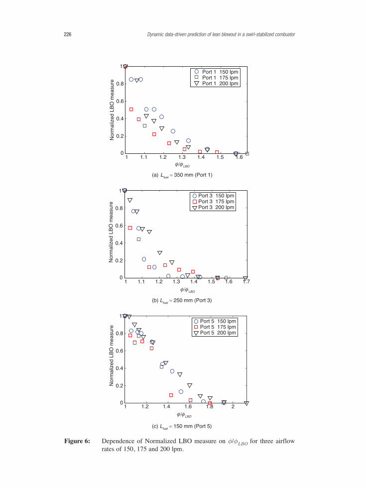
Figures 6(a), 6(b), and 6(c) show the performance of the proposed LBO measure forthree different flow rates (i.e., 150, 175 and 200 lpm) at well-premixed (Port 1),partially-premixed (Port 3), and poorly-mixed (Port 5) fuel-air conditions, respectively.It is seen that, with the exception of the poorly-mixed condition (i.e., Lfuel = 150 mm(Port 5)), the average slope of the normalized LBO measure with respect to normalizedequivalence ratio (φ/φLBO) remains low till φ/φLBO reaches 1.2. As φ/φLBO is reducedbelow 1.2, the slope of the normalized LBO measure starts increasing rapidly even forthe well-premixed condition, as seen in Figure 6(a). Below φ/φLBO = 1.1, thenormalized LBO measure attains a value in the range of 0.4 – 0.6 and it reaches 1 witha steep slope when the flame blows out. The steep rise in slope of the normalized LBOmeasure close to LBO (φ/φLBO < 1.2) is desirable, because a sensitive LBO measurewould be capable of detecting the proximity of LBO. It is apparent from Figure 6(c) thatthe normalized LBO measure for the poorly-mixed is not as sensitive as it is in the cases



1 1.1 1.2 1.3 1.4 1.5 1.60

0.2

0.4

0.6

0.8

1

(a)

(b)

(c)

φ/φLBO

Nor

mal

ized

LB

O m

easu

re

Lfuel = 150 mm (Port 5)

Port 1 150 lpmPort 1 175 lpmPort 1 200 lpm

1 1.1 1.2 1.3 1.4 1.5 1.6 1.7

Nor

mal

ized

LB

O m

easu

re


φ/φLBO

0

0.2

0.4

0.6

0.8

1

1 1.2 1.4 1.6 1.8 2

Nor

mal

ized

LB

O m

easu

re


φ/φLBO

0

0.2

0.4

0.6

0.8

1



Figure 6: Dependence of Normalized LBO measure on φ/φLBO for three airflowrates of 150, 175 and 200 lpm.

of well-premixed and partially-premixed conditions. The rationale for this result can beattributed to the absence of dominant precursor events prior to LBO at a poorly-premixed condition.

Subsequently, the ensemble of time series data for these three air-flow rates aremixed to build a robust classification scheme, where it is ensured that such data setswere independently collected. Since the number of samples in each class is not large(e.g., 10), leave-one-out cross-validation approach is adopted for LBO prediction andsupport vector machines (SVM) with linear kernels [34] are used at both first andsecond levels of classification (see Figure 4). The results of this classification methodare presented in Table I using confusion matrices for three different premixing lengths,where the rows are the actual classes (i.e., ground truth) and the columns are thepredicted classes. [Note: the notions of two classes of alarm, namely, Impending LBO(ILBO) and Progressive LBO (PLBO) have been introduced in Subsection 3-B5]. Table I shows high accuracy in detecting ILBO, PLBO, and nominal conditions withlarger air-fuel premixing (i.e., higher values of Lfuel)).

The confusion matrices in Table I show that the D-Markov machine is capable ofclassifying different LBO situations fairly accurately even in the absence of intensevisual flame-precursor events. The efficacy of the proposed method to detect LBO evenat low levels of premixing is important as other methods reported in literature mostlydeal with lean premixed flames and do not generally work very satisfactorily forpartially premixed configurations [12]. This classification scheme, in general, predictsthe proximity of LBO fairly accurately for a wide range of air-flow rate,

The D-Markov machine parameters of the pattern classifier are now presented forLBO prediction for well-premixed, partially-premixed, and poorly premixed fuel-airflow.

1) LBO Prediction for Premixed Flame: For combustion flames with fuel flow fromPort 1 (i.e., Lfuel = 350 mm) and Port 3 (i.e., Lfuel = 250 mm) are at well-premixed andpartially-premixed conditions, respectively. The D-Markov machine parameters arefound to be the same for these cases.

The symbol alphabet is = {1, 2, 3, 4, 5, 6, 7}, i,e,, the alphabet size is || = 7.After state merging, the states of the D-Markov machine are calculated for the


Table 1: Confusion matrix before lean blow out for differet premixing (port 1, port 3 and port 5)

PREDICTED

A Premixing level Port 1 (Lfuel = 350 mm) Port 3 (Lfuel = 250 mm) Port 5 (Lfuel = 150 mm)

C Alarm Alarm Alarm

T Class ILBO PLBO Nom ILBO PLBO Nom ILBO PLBO Nom

U ILBO 9 0 0 9 0 0 6 2 0

A Alarm PLBO 0 7 0 0 6 0 0 6 0

L Nom 0 1 12 0 1 12 0 3 16

stoichiometric fuel/air ratio, i.e., φ = 1, are found to be eleven (i.e., |Q| = 11) for thedata from Port 1 and Port 3. The corresponding sets of states are: {1, 2, 3, {14, 24}, 34,44, 54, {64, 74}, 5, 6, 7} and {1, 2, 3, 4, {15, 75}, {25, 35}, 45, 55, 65, 6, 7} for port 1 and port 3, respectively.

2) LBO Prediction for Non-Premixed Flame: Combustion flame with fuel flow fromport 5 (Lfuel = 150 mm) is close to non-premixed condition. The alphabet size is keptat || = 7. After state merging, the number of states for the D-Markov machine iscalculated (based on φ = 1) to be eleven. Figure 6(c) shows the performance of theproposed LBO measure for different flow rates at a (nearly) non-premixed condition.

D. Performance of D-Markov Machine: D = 1 and D > 1D-Markov machines with D = 1 was reported by Chaudhuri [23] and Mukhopadhyayet al. [12] to perform equivalently or sometime superior to other time series basedonline LBO prediction tools [6], [7], [8], [9], [10]. This subsection makes a comparisonof the predictive performance of D-Markov machines for D > 1 with that for D = 1,which was reported earlier for LBO prediction [12]. This comparison is performedbased on the following two metrics.

1) Total mis-prediction = (Actual ILBO, predicted PLBO) + (Actual ILBO,predicted Nominal) + (Actual PLBO, predicted Nominal); and

2) Total false alarm = (Actual Nominal, predicted PLBO) + (Actual Nominal,predicted ILBO) + (Actual PLBO, predicted ILBO).

Figure 7 shows how the classification performance is improved for a typical case ofcombustion with fuel inlet at port 5 (see Figure 1), as the number of PFSA states |Q| inthe D-Markov machine is increased via state splitting and state merging for an alphabet


5 10 15 200

0.2

0.4

0.6

0.8

1

Number of states

Pre

dict

ive

perf

orm

ance

Classification accuracy

Total mis−prediction

Total false alarm

Figure 7: Dependence of predictive performance of the D-Markov machine on thenumber of states (|Q|) from alphabet size || = 5.

size || = 5. It appears that the predictive performance of the D-Markov machinesaturates beyond a certain value of number of states (e.g., |Q| = 10), as seen in Figure 7. Investigation of the fact, whether the phase space dimension of thecombustion dynamics consistently converges in the vicinity of LBO, is a topic of futureresearch as indicated in Section 5.

Table II shows that the classification performance of the D-Markov machine with D > 1 becomes increasing better relative to that of its predecessor with D = 1 as thequality of premixing is degraded. For higher premixing, the performances of Port 1 andPort 3 are comparable, which is intuitively supported by the presence of intense andclearly visible precursor events before the onset of LBO. However, as the quality offuel-air premixing is reduced (e.g., Port 5), the visibility of precursor events becomesrather rare. This physical phenomenon makes the task of LBO prediction more difficult.The last row of Table II shows that the the D-Markov machine with D > 1 performswell for all ports including Port 5 too, whereas the D-Markov machine with D = 1 failsto predict LBO as it yields unacceptable levels of total mis-predictions and total falsealarms. The technique adopted in [12] (that uses D = 1) may not perform satisfactorilywhen the bias due to the mean value of the CH* chemiluminescence is removed fromthe analyzed signal. Although the usage of D = 1 may work in presence of the bias,mean-based implementations could lead to higher emission as discussed earlier. Thus,the development and validation of the D-Markov machine with D > 1 for LBOprediction is one of the major contributions of the present work.

E. Estimate of the Computational CostThe computational cost of the proposed algorithm is estimated for calculating the LBOmeasure from the time series of raw chemiluminescence data on a Dell Precision T3400platform with Intel(R) Core(TM) 2 Quad CPU Q9550 @ 2.83 GHz 2.83 GHz. The statespace of the PFSA is usually constructed off-line via state splitting and state merging.Figure 8 shows the profiles of required computational time (in the MATLAB 7.10.0(R2010a) environment) to obtain the LBO measure from a one-second-duration timeseries of raw chemiluminescence data, collected at a sample frequency of 2 kHz. The


Table 2: Performance comparison oflbo prediction by D-Markovmachine classification with D > 1 and D = 1)

Port # Total mis- Total false(# of test cases) predictions alarms

Port 1 (29) D > 1 0 1D = 1 2 3

Port 3 (28) D > 1 0 1D = 1 4 4

Port 5 (33) D > 1 2 3D = 1 6 9

equality of alphabet size || and number of PFSA states |Q| > at the beginning of eachplot in Figure 8 implies D = 1; for subsequent points in each plot, |Q| > ||, whichimplies that state splitting and merging with D > 1. It is seen that the computationaltime has an increasing trend as the depth D of the underlying PFSA (see Definition 3.1)is increased from one. A typical value of computational time is 20 ms for the alphabetsize || = 7 and the number of PFSA states |Q| = 11. Apparently, the proposed methodof LBO prediction is well-suited for real-time LBO prediction, where the typicalfrequency response of combustion dynamics is 10 Hz [18].

5. SUMMARY, CONCLUSIONS AND FUTURE WORKThis paper addresses data-driven pattern classification for prediction of lean blowout(LBO) phenomena in combustion processes. The proposed LBO prediction method isbuilt upon low-dimensional feature vectors that are extracted from time series of opticalsensor data of chemiluminescence. The feature vectors are realized as (statisticallystationary) state probability vectors of a special class of finite-history probabilisticfinite state automata (PFSA). These PFSA, called D-Markov machines, have adeterministic algebraic structure and their states are represented by symbol blocks oflength D or less, where D is a positive integer. The states of a D-Markov machine areconstructed via splitting the symbol blocks of different lengths based on theirinformation contents and merging two or more split states without any significant lossof the embedded information.

An anomaly measure, based on Kullback-Leibler divergence, is constructed tosuccessfully predict the onset of LBO. This anomaly measure becomes increasinglysensitive to small changes in the equivalence ratio as the combustion process


6 8 10 12 14 16 18 20 220.014

0.016

0.018

0.02

0.022

0.024

Number of states |Q|

Tim

e (s

ec)

Alphabet size ⎪Σ⎪ = 5 Alphabet size ⎪Σ⎪ = 6 Alphabet size ⎪Σ⎪ = 7

Figure 8: Computation times for calculating LBO measure from 1 second of rawchemiluminescence time series (sampling frequency 2 kHz) for differentnumber of states |Q| and different alphabet size ||.

approaches LBO. An architecture of the pattern classification problem has beenformulated based on different ranges of the equivalence ratio to reliably predict theLBO optimally ahead of its onset. The proposed pattern classification method has beenvalidated on experimental data collected from a laboratory-scale swirl-stabilizedcombustor. It is observed that the modeling complexity (i.e., number of states of D-Markov machine) of the PFSA, constructed from optical sensor data reduces drasticallyas the system approaches LBO.

It is demonstrated over a wide range of fuel-air premixing and air flow rates that theD-Markov machine with D > 1 performs significantly better than the D-Markovmachine with D = 1 for prediction of LBO [12]. The results, reported in this paper,suggest the potential capability of D-Markov machines to fairly precisely predictregions close to LBO in a laboratory- scale combustor. In this way, the operatingcondition in a combustor could be extended to a leaner equivalence ratio withoutsignificantly risking LBO. While there are many other areas yet to be addressed in thiscontext, a few topics of future research are delineated below.

1) Theoretical research on identification of the optimum threshold for maximumnumber of states (state splitting) and the distance metric (state merging) forenhancement of the predictive performance of the D-Markov machine.

2) Prediction of combustion instability in both premixed and non-premixedcombustors.

3) Prediction of LBO under thermo-acoustic instability for different flowconditions.

4) Validation of the proposed data-driven approach with respect to model-driventools.

5) Identification of the statistical ranges of uncertainty in the LBO measure (e.g.,relative to different confidence levels) in typical combustors.

6) Investigation of the physical significance of the reduction in number of D-Markov machine states in the vicinity of LBO relative to the correspondingchanges in the dynamic behavior of the combustion system under nominaloperating conditions.

7) Theoretical and experimental research on prediction of thermo-acousticinstabilities under operating conditions, other than LBO (e.g., screechphenomena in the afterburner of gas turbine engines in tactical aircraft [41]).

ACKNOWLEDGEMENTSThe work reported in this paper has been supported in part by the U.S. Air Force Officeof Scientific Research under Grant No. FA9550-12-1-0270, by the U.S. Office of NavalResearch under Grant No. N00014-14-1-0545, and by the U.S. Army ResearchLaboratory under Grant No. W911NF-14-2-0068. Any opinions, findings andconclusions or recommendations expressed in this publication are those of the authorsand do not necessarily reflect the views of the sponsoring agencies. The authorsthankfully acknowledge the benefits of scientific and technical discussions with theircolleagues in the following areas:


• Dr. K. Mukherjee and Dr. S. Phoha of Pennsylvania State University fordevelopment of the theory of the D-Markov machine.

• Professor S. Chakravarthy and Professor R.I. Sujith of Indian Institute ofTechnology, Madras for interpretation of the physical phenomena of combustion.

APPENDIX ACONCEPT OF TWO TIME SCALESThis appendix presents the notion of two time scales in dynamical systems, as neededfor pattern classification based on time series of sensor data.

Definition A.1 (Fast Scale) The fast scale is defined to be a time scale over whichthe statistical properties of the process dynamics are assumed to remain invariant, i.e.,the process is assumed to have statistically stationary dynamics at the fast scale.

Definition A.2 (Slow Scale) The slow scale is defined to be a time scale over whichthe statistical properties of the process dynamics may gradually evolve, i.e., the processmay exhibit statistically non-stationary dynamics at the slow scale.

In view of Definition A.1, statistical variations in the internal dynamics of theprocess are assumed to be negligible at the fast scale. Thus, sensor time series data areacquired based on the assumption of statistical stationarity at the fast scale. In view ofDefinition A.2, an observable non-stationary behavior could be associated with thegradual evolution of anomalies (i.e., deviations from the nominal behavior) in theprocess at the slow scale. In general, a long time span at the fast scale is a tiny (i.e.,several orders of magnitude smaller) interval at the slow scale. A pictorial view of thetwo-time-scales operation in Figure 9 illustrates the concept.

APPENDIX BMATHEMATICAL PRELIMINARIESThis appendix presents pertinent information regarding construction of D-Markovmachines and other mathematical tools (e.g., entropy rate and metric to quantify thedistance between two PFSA). The following standard definitions are recalled [14].

Definition B.1 (Finite State Automaton) A finite state automaton (FSA) G, having adeterministic algebraic structure, is a triple (, Q, δ) where:


Slow time epochs

τ1 τ2τ3 τ4

Fast time instants

Figure 9: Underlying concept of fast and slow time scales.

• is a (nonempty) finite alphabet with cardinality ||;• Q is a (nonempty) finite set of states with cardinality |Q|;• δ : Q Q is a state transition map.Definition B.2 (Symbol Block) A symbol block, also called a word, is a finite-length

string of symbols belonging to the alphabet , where the length of a word

with si is |w| = �, and the length of the empty word ε is |ε| = 0. The parameters ofFSA are extended as:

• The set of all words constructed from symbols in , including the empty word ε,is denoted as *,

• The set of all words, whose suffix (respectively, prefix) is the word w, is denoted as*w (respectively, w*).

• The set of all words of (finite) length �, where � > 0, is denoted as �.Definition B.3 (Extended Map) The extended state transition map δ* : Q * Q

transfers one state to another through finitely many transitions such that, for all q Q,σ and w *,

where wσ is the suffixing of the word w by the symbol .Definition B.4 (Irreducible FSA) An FSA G is said to be irreducible if, for all q1 , q2

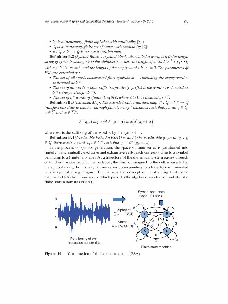
Q, there exists a word w1,2 * such that q1 = δ* (q2, w1,2).In the process of symbol generation, the space of time series is partitioned into

finitely many mutually exclusive and exhaustive cells, each corresponding to a symbolbelonging to a (finite) alphabet. As a trajectory of the dynamical system passes throughor touches various cells of the partition, the symbol assigned to the cell is inserted inthe symbol string. In this way, a time series corresponding to a trajectory is convertedinto a symbol string. Figure 10 illustrates the concept of constructing finite stateautomata (FSA) from time series, which provides the algebraic structure of probabilisticfinite state automata (PFSA).

� � �w s s s1 2

δ δ σ δ δ σ( )( ) ( )= =∈q q and q w q w, , ( , ),* * *


Figure 10: Construction of finite state automata (FSA)

Partitioning of pre−processed sensor data

Finite state machine

Symbol sequence

0

0

00

0

1

11

1 1

2

2

2 2

2

3

3

33

3

...232211011223...

States Q = {A,B,C,D}

Alphabet ∑ = {1,2,3,4}

Definition B.5 (PFSA) A probabilistic finite state automaton (PFSA) K is a pair (G, π), where:

• The deterministic FSA G is called the underlying FSA of the PFSA K;• The probability map π : Q [0, 1] is called the morph function (also known

as symbol generation probability function) that satisfies the condition:for all q Q.

Equivalently, a PFSA is a quadruple K = ( , Q, δ, π), where• The alphabet of symbols is a (nonempty) finite set, i.e., 0 < || < ∞, where ||

is the cardinality of ;• The set Q of automaton states is (nonempty) finite, i.e., 0 < |Q| < ∞, where |Q|

is the cardinality of Q;• The state transition function δ : Q Q;• The morph function π : Q [0, 1], where for all q Q.

The morph function π generates the (|Q| ||)morph matrix P.

Definition B.6 (Extended Morph Function) The morph function π : Q [0, 1]of PFSA is extended as π* : Q * [0, 1] such that, for all q Q, σ and w *,

where w is the suffixing of the word w by the symbol . The above equationsrepresent how the PFSA responds to occurrence of a certain block of symbols, i.e, aword w * of finite length |w|.

A. Symbolization of Time SeriesThis step requires partitioning (also known as quantization) of the time series data ofthe measured signal. The signal space is partitioned into a finite number of cells that arelabeled as symbols, i.e., the number of cells is identically equal to the cardinality ||of the (symbol) alphabet . As an example for the one-dimensional time series in Figure 10, the alphabet = {α, β, γ , δ}, i.e., || = 4, and three partitioning linesdivide the ordinate (i.e., y-axis) of the time series profile into four mutually exclusiveand exhaustive regions. These disjoint regions form a partition, where each region islabeled with one symbol from the alphabet . If the value of time series at a giveninstant is located in a particular cell, then it is coded with the symbol associated withthat cell. As such, a symbol from the alphabet is assigned to each (signal) valuecorresponding to the cell where it belongs. (Details are reported in [31].) Thus, a (finite)array of symbols, called a symbol string (or symbol block), is generated from the(finite-length) time series data.

The ensemble of time series data are partitioned by using a partitioning tool (e.g.,maximum entropy partitioning (MEP) or uniform partitioning (UP) methods [31]). InUP, the partitioning lines are separated by equal-sized cells. On the other hand, MEPmaximizes the entropy of the generated symbols and therefore, the information-rich

π π σ π π δ σ( )( ) ( )= = ×∈q and q w q w q w, 1 , ( , ) ( , ),* * * *

∑ π σ =σ∈Σ

q( , ) 1

∑ π σ =σ∈Σ

q( , ) 1


cells of a data set are partitioned finer and those with sparse information are partitionedcoarser, i.e., each cell contains (approximately) equal number of data points under MEP.In both UP and MEP, the choice of alphabet size || largely depends on the specificdata set and the allowable loss of information (e.g., leading to error of detection andclassification).

1) Selection of Alphabet Size: Considerations for the choice of alphabet size ||include the maximum discrimination capability of a symbol sequence and theassociated computational complexity. The maximum discrimination capability ischaracterized by the entropy of the sequence that should be maximized to the extent itis possible, or alternatively by minimizing the information loss that is denoted as thenegative of the entropy. As the alphabet size is increased, there is both an increase incomputational complexity and a possible reduction in loss of information; in addition,the effects of a large alphabet may become more pronounced for an insufficiently longtime series [22].

In partitioning of a (one-dimensional) time series for symbolization, the alphabetsize || must be appropriately chosen in order to transform the real-valued finite-lengthdata set S into a symbol string. The data set S is partitioned into a (finite) number of(mutually exclusive and exhaustive) segments to construct a mapping between S andthe alphabet of symbols {s|s }. To do so, a choice must be made as to the numberof symbols, i.e., the cardinality || of the symbol alphabet . Presented below is a briefdiscussion on how to make the tradeoff between information loss and computationalcomplexity.

Let the alphabet size be k = || and the method of partitioning the time series bemaximum entropy partitioning [31], i.e., a uniform probability distribution on the

symbols with Then, the information loss, represented by the

negative of the entropy [21] of the symbol sequence, is given as

(11)

By representing the computational complexity as a function g(k) of the alphabet sizek and choosing an appropriate scalar tradeoff weighting parameter a (0, 1), the costfunctional to be optimized becomes:

(12)

The optimal alphabet size || is obtained by solving for k in the equation J(k + 1) -J(k) = 0 along with additional constraints that may have to be imposed in theoptimization procedure to realize the effects of critical issues such as any bounds on thealphabet size.

B. Entropy rateThis subsection introduces the notion of entropy rate that, given the current state,represents the predictability of PFSA.

σ σ( ) = ∀ ∈ ∑Pk1

.

σ σ( ) ( )=− = ∑ =−σ∈∑I H P P kIn In

α α( ) ( ) ( )=− + −J k k g kIn 1


Definition B.7 (Conditional Entropy and Entropy Rate [21]) The entropy of a PFSA(, Q, δ, π) conditioned on the current state q Q is defined as follows.

(13)

The entropy rate of a PFSA (, Q, δ, π) is defined in terms of the conditionalentropy as follows.

(14)

where P(q) is the (unconditional) probability of a PFSA state q Q; and P( |q) is the(conditional) probability of a symbol σ emanating from the PFSA state q Q.

C. Metric for the distance between two PFSAThis subsection introduces the notion of a metric to quantify the distance between twoPFSA.

Definition B.8 (Metric) Let K1 = (, Q1, δ1, π1) and K2 = (, Q2, δ2, π2) be twoPFSA with a common alphabet . Let P1(

j) and P2(j) be the steady state

probability vectors of generating words of length j from the PFSA K1 and K2,respectively, i.e., P1(

j) � [P(w)]wj for K1 and P2(j) � [P(w)]wj for K2. Then,

the metric for the distance between the PFSA K1 and K2 is defined as

(15)

where the norm ||*||�1 indicates the sum of absolute values of the elements in the vector *.The norm on the right side of Eq. (15) yields

because each of the probability vectors P1(j) and P2(

j) has non-negative entries thatsum to 1. Furthermore, convergence of the infinite sum on the right side of Eq. (15) is

guaranteed due to the weight and satisfies the relation 0 F(, ) 1. It is noted

that alternative forms of norms could also be used, because of norm equivalence infinite-dimensional vector spaces.

Since the metric in Definition B.8 assigns more weight to words of smaller length,the infinite sum could be truncated to a relatively small order D (e.g., typically in therange of 5 to 20) [31] for a given tolerance ε � 1. That is, the distance F(, ) in Eq. (15) effectively compares the probabilities of generating words of length D in two

� ∑ σ σ( ) ( )( )∑⎞

⎠⎟⎟⎟⎟σ∈∑

H q P q P qlog

�∑

∑∑ σ σ

( ) ( )

( ) ( )

( )

( )

∑ ∑

=−σ

∈

∈∑∈

H Q P q H q

P q P q P qlog

q Q

q Q

� �∑( ) ( )

( )Φ∑ − ∑

→∞ +=

K KP P

, lim2n

j j

jj

n

1 2

1 2

11

1

� � �( ) ( ) ( ) ( )∑ − ∑ ≤ ∑ + ∑ =P P P P 2j j j j

1 2 1 21 1 2

+

12 j 1


PFSA and is especially adaptable to D-Markov machines whose dynamical behavior ischaracterized by words of a specified maximal depth [13].

The metric F(, ) can also be used to calculate the distance between a PFSA and asymbol string, in which case the probabilities are expressed in terms of relativefrequency of occurrence of a word.

APPENDIX CSTATE SPLITTING & STATE MERGING ALGORITHMSThis appendix lists the algorithms of state splitting and state merging for constructionprobabilistic finite state state automata (PFSA) from symbol strings, where statesplitting is addressed by Algorithm 1 and state merging by Algorithms 2, 3 and 4.

Algorithm 1 State splittingInput: Symbol sequence s1s2s3....., where each si belongs

to the symbol alphabet User defined Parameters: Maximum number of states Nmax and

threshold ηspl for state splittingOutput: PFSA K = {, Q, δ, π}Initialize: Create a 1-Markov machine := repeat

Q := ;

= arg minQ H(|Q);where Q = (Q\{q}) ({σq : σ }) and q Q

until | | < Nmax or H(|Q) - H(| ) < ηspl

for all and σ do

if δ(q, ) is not unique then

:= ( \{q}) ({σq : σ });end if

end forreturn K = {, Q, δ, π}

Algorithm 2 Minimal equivalence relation given q qInput: δ, q, q, Initial equivalence relation Output: Updated equivalence relation NOTE: Recursive function () := Merge(δ, q, q, )Set q q;for all σ do

if δ(q, σ) δ(q, σ) then

Set := Merge(δ, δ(q, σ), δ(q, σ), );

end ifend forreturn

�Q

�Q�Q

�Q

�∈q Q

�Q�Q

�Q


Algorithm 3 Minimal PFSA K2 after merging of two states

Input: K1 = {, Q1, δ1, π1}, q, qOutput: Merged PFSA K2 = {, Q2, δ2, π2}Compute the equivalence relation using Algorithm 2;Set Q2 := Q1/ ; % Q2 is the quotient set of Q1 under Compute the stationary-probability vector P̂1 of the PFSA K1;for all [q] Q2 do

for all σ doSet δ2([q], σ) := [δ1(q, σ)];Compute p2([q], σ) using Eq. (7);

end forend forreturn K2 = {, Q2, δ2, π2}

Algorithm 4 State merging in PFSAInput: PFSA K = {, Q, δ, π} and symbol sequence {si}User defined Parameter: Threshold ηmrg for state mergingOutput: Merged PFSA Km = {, Qm, δm, πm}Set Km := K;for all q, q Qm do

if q ≠ q thenSet LIST STATES (q, q) = M(q, q) using Eq. (9);

elseSet LIST STATES (q, q) = 2;

end ifend forsort (LIST STATES); % Place the pair (q, q) with the smallest M(q, q) on top ofthe listSet (q, q) := pop (LIST STATES); % Select the pair (q, q) that is on top of thesorted listloop

Compute K1 from Km by merging the states q and q via Algorithm 3;if d [K1, {si}] < mrg then

Set Km := K1;Recompute LIST STATES;Set (q, q) := pop (LIST STATES);

else

Set (q, q) := pop (LIST STATES);if q = q then

Break loop;end if

end ifend loopreturn Km = {, Qm, δm, πm}


REFERENCES[1] S. D. Zilwa, J. H. Uhm, and J. H. Whitelaw, “Combustion oscillations close to the

lean flammability limit,” Combustion Science and Technology, 2000, 160,231–258.

[2] S. Chaudhuri and B. M. Cetegen, “Blowoff characteristics of bluff body stabilizedconical premixed flames under upstream mixture gradients and velocityoscillations,” Combustion and Flame, 2008, 153, 616–633.

[3] S. Chaudhuri and B. M. Cetegen, “Blowoff characteristics of bluff body stabilizedconical premixed flames in a duct with upstream mixture gradients and velocityoscillations,” Combustion Science and Technology, 2009, 181, 555–569.

[4] S. Chaudhuri, S. Kostska, M. W. Renfro, and B. M. Cetegen, “Blowoff dynamicsof bluff body stabilized turbulent premixed flames,” Combustion and Flame,2010, 157, 790–802.

[5] M. Stohr, I. Boxx, C. Carter, and W. Meier, “Dynamics of lean blowout of a swirl-stabilized flame in a gas turbine model combustor,” Proceedings of theCombustion Institute, 2011, 33, 2953 2960.

[6] S. Nair, T. M. Muruganandam, R. Olsen, A. Meyers, J. Seitzman, B. T. Zinn, T. Lieuwen, T. Held, and H. Mongia, “Lean blowout detection in a single nozzleswirl cup combustor,” in 42nd AIAA Aerospace Sciences Meeting and Exhibit,Reno, NV, USA, 2004, AIAA 2004–0138.

[7] T. M. Muruganandam, S. Nair, D. Scarborough, Y. Neumeier, J. Jagoda, T. Lieuwen, J. Seitzman, and B. T. Zinn, “Active control of lean blowout forturbine engine combustors,” Journal of Propulsion and Power, 2005, 21,807–815.

[8] S. Nair and T. Lieuwen, “Acoustic detection of blowout in premixed flames,”Journal of Propulsion and Power, 2005, 21, 32–39.

[9] S. Prakash, S. Nair, T. M. Muruganandam, Y. Neumeier, T. Lieuwen, J. M.Seitzman, and B. T. Zinn, “Acoustic based rapid blowout mitigation in a swirlstabilized combustor,” in ASME Turbo Expo, Reno, USA, 2005.

[10] T. Yi and E. J. Gutmark, “Real-time prediction of incipient lean blowout in gasturbine combustors,” AIAA Journal, 2007, 45, 1734–1739.

[11] R. R. Chaudhari, R. Sahu, S. Ghosh, A. Mukhopadhyay, and S. Sen, “Flame coloras a lean blowout predictor,” International Journal of Spray and CombustionDynamics, 2013, 5, 49–66.

[12] A. Mukhopadhyay, R. Chaudhuri, T. Paul, S. Sen, and A. Ray, “Prediction of leanblow-out in gas turbine combustors using symbolic time series analysis,” Journalof Propulsion and Power (AIAA), 2013, 29, 950–960.

[13] A. Ray, “Symbolic dynamic analysis of complex systems for anomaly detection,”Signal Processing, July 2004, 84, 1115–1130.

[14] K. Mukherjee and A. Ray, “State splitting and state merging in probabilistic finitestate automata for signal representation and analysis,” Signal Processing,November 2014, 104, 105–119.


[15] L. Kabiraj, R. I. Sujith, and P. Wahi, “Investigating dynamics of combustiondriven oscillations leading to lean blowout,” Fluid Dynamics Research, 2012, 44.

[16] L. Kabiraj and R. I. Sujith, “Nonlinear self-excited thermoacoustic oscillations:intermittency and flame blowout,” J. Fluid Mech., 2012, 713, 376–397.

[17] H. Gotoda, M. Amano, T. Miyano, T. Ikawa, K. Maki, and S. Tachibana,“Characterization of complexities in combustion instability in a lean premixedgas-turbine model combustor,” Chaos, 2012, 22, 043128.

[18] H. Gotoda, Y. Shinoda, M. Kobayashi, Y. Okuno, and S. Tachibana, “Detectionand control of combustion instability based on the concept of dynamical systemtheory,” Phys. Rev. E, 2014, 89, 022910.

[19] V. Nair, G. Thampi, S. Karuppusamy, S. Gopalan, and R. I. Sujith, “Loss of chaosin combustion noise as a precursor of impending combustion instability,”International Journal of Spray and Combustion Dynamics, 2013, 5, 273–290.

[20] F. Darema, “Dynamic data driven applications systems: new capabilities forapplication simulations and measurements”. In: 5th International conference oncomputational science – ICCS 2005, Atlanta, GA (United States); May 2005, 610-615.

[21] T. Cover and J. Thomas, Elements of Information Theory, 2nd ed. Hoboken, NJ,USA: Wiley, 2006.

[22] Y. Wen, K. Mukherjee, and A. Ray, “Adaptive pattern classification for symbolicdynamic systems,” Signal Processing, 2013, 93, 252–260.

[23] R. Chaudhari, Investigation of Thermoacoustic Instabilities and Lean Blowout ina Model Gas Turbine Combustor. PhD thesis, Jadavpur University, India, 2011.Ph.D. Dissertation, Department of Mechanical Engineering.

[24] T. Williams, R. Schefer, J. Oefelein, and C. Shaddix, “Idealized gas turbinecombustor for performance research and validation of large eddy simulations,”Review of Scientific Instruments, 2007, 78, 035114–1–9.

[25] W. Meier, P. Weigand, X. Duan, and R. Giezendanner-Thobben, “Detailedcharacterization of the dynamics of thermoacoustic pulsations in a lean premixedswirl flame,” Combustion and Flame, 2007, 150, 2–26.

[26] S. Turns, An Introduction to Combustion. NYC, NY, USA: McGraw-Hill, 2 ed.,2000.

[27] C. Daw, M. Kennel, C. Finney, and F. Connolly, “Observing and modelingnonlinear dynamics in an internal combustion engine,” Physical Review. E, 1998,57, 2811 2819.

[28] D. Lind and B. Marcus, Symbolic Dynamics and Coding. Cambridge UniversityPress, Cambridge, UK, 1995.

[29] P. Dupont, F. Denis, and Y. Esposito, “Links between probabilistic automata andhidden Markov models: probability distributions, learning models and inductionalgorithms,” Pattern Recognition, 2005, 38, 1349–1371.


[30] E. Vidal, F. Thollard, C. de la Higuera, F. Casacuberta, and R. Carrasco,“Probabilistic finite-state machines - Part I and Part II,” IEEE Transactions onPattern Analysis and Machine Intelligence, 2005, 27, 1013–1039.

[31] V. Rajagopalan and A. Ray, “Symbolic time series analysis via wavelet-basedpartitioning,” Signal Processing, 2006, 86, 3309–3320.

[32] C. Rao, A. Ray, S. Sarkar, and M. Yasar, “Review and comparative evaluation ofsymbolic dynamic filtering for detection of anomaly patterns,” Signal, Image andVideo Processing, 2009, 3, 101–114.

[33] S. Bahrampour, A. Ray, S. Sarkar, T. Damarla, and N. Nasrabadi, “Performancecomparison of feature extraction algorithms for target detection andclassification,” Pattern Recogntion Letters, December 2013, 34, 2126–2134.

[34] C. M. Bishop, Pattern Recognition and Machine Learning. Springer, New York,NY, USA, 2006.

[35] T. Liao, “Clustering of time series data – A survey,” Pattern Recognition, 2005,38, 1857–1874.

[36] C. Shalizi and K. Shalizi, “Blind construction of optimal nonlinear recursivepredictors for discrete sequences,” in AUAI ‘04: Proceedings of the 20thConference on Uncertainty in Artificial Intelligence, (Arlington, VA, USA),AUAI Press, 2004, 504–511.

[37] M. Sipser, Introduction to the Theory of Computation, 3rd ed. Boston, MA, USA:Cengage Publishing, 2013.

[38] G. Mallapragada, A. Ray, and X. Jin, “Symbolic dynamic filtering and languagemeasure for behavior identification of mobile robots,” IEEE Transactions onSystem, Man, and Cybernetics Part B: Cybernetics, June 2012, 42, 647–659.

[39] C. Beck and F. Schlӧgl, Thermodynamics of chaotic systems: an introduction.Cambridge, U.K: Cambridge University Press, 1993.

[40] P. Halmos, Naive Set Theory, 26–29. Princeton, NJ: Van Nostrand, 1960.

[41] H. Ebrahimi, “Overview of gas turbine augmentor design, operation andcombustion oscillation,” in ILASS Americas, 19th Annual Conference on LiquidAtomization and Spray Systems, Toronto, Canada, 2006.


Date post:	17-Apr-2018
Category:	Documents
Upload:	dinhminh
View:	219 times
Download:	0 times

Dynamic data-driven prediction of lean blowout in a … data-driven prediction of lean blowout in a...

Documents