Dynamic Effects of Total Debt and GDP: A Time-Series Analysis of the United States Economics Master's thesis Patrizio Lainà 2011 Department of Economics Aalto University School of Economics
Transcript
Dynamic Effects of Total Debt and GDP: A Time-SeriesAnalysis of the United States
Economics
Master's thesis
Patrizio Lainà
2011
Department of EconomicsAalto UniversitySchool of Economics
Although nowadays most economists agree that money is created endogenously, there exist
different perspectives on how much control central banks have over the money supply and loans in
general. The two common approaches are accommodationist view and structuralist view. The
accommodationist view maintains that central banks are always willing to fully accommodate the
commercial banks' need for reserves. In addition, it suggests that the money supply is not controlled
through the monetary base, but through the interest rates. Thus, the central bank money supply
function is horizontal in money-interest space. The structuralist view holds that central banks do not
accommodate the needed reserves fully. It also holds that central banks can control the money
supply through the monetary base, if they choose so, but conclude that mostly they do not. Thus, the
central bank money supply function is upward sloping in money-interest space. It is, however,
possible that both views are accurate. The accommodationist view could be an accurate description
of the short-run money supply, while the structuralist view could be a plausible explanation of the
intermediate-run money supply.
We will not go deeper into these different approaches as they are beyond the scope of this study, but
some empirical studies to support or to reject these approaches are briefly presented below. We
already discussed the findings of Kydland and Prescott (1990) that the exogenous money creation
theory does not hold in reality. However, they did not explicitly study endogenous money, although
their results support it. Moore (1989) studies the endogenous money creation theory in the United
States and finds evidence to support the accommodationist view. The findings of Pollins (1991), on
the other hand, support the structuralist view over the accommodationist approach. Shanmugan,
Nair and Li (2003) study and compare the different approaches in Malaysia between 1985 and
2000. The results support the accommodationist view, but not the structuralist view, although it
could neither be rejected. Vera (2001) collects data from Spain from 1987 until 1998. The results
provide some evidence for both views, but not enough in order to discriminate between them.
Tarvonen (2011) finds strongest evidence for the accommodationist view, but no evidence supports
the structuralist view.
Although there still seems to be dispute which approach of the endogenous money creation theory
24
is correct, there seems to be a consensus that money, regardless of the details, is endogenous. The
next two sections will present two branches of the endogenous money creation theory. First, the
modern money theory, which focuses on the role of central bank money, is presented. Then, the
monetary circuit theory, which describes how production takes place from the perspective of money
and debt, is presented.
3.3 Modern money theory
This section explains the modern money theory, or chartalism. It maintains that money mainly
derives its value from the government’s ability to levy taxes denominated in the currency it chooses
and issues. The modern money theory is also sometimes called as the state theory of money because
it emphasizes the role of central bank money over commercial bank money. It stresses that
commercial banks can create money, but the payments between banks always have to be cleared
solely with central bank money. This fact raises a need to scrutinize our payment system and the
role of central bank money in it.
Although modern money theory has not established its position among the mainstream economic
theory, its roots are long. Knapp (1924) is seen as the founder of the modern money theory already
in 1905. Also Innes (1913) is an important early contributor. Later, the approach experienced a
revival under Lerner (1947). The approach influenced also Keynes (1971) as he positively cites
Knapp and chartalism in the opening pages. Contemporaneous proponents include, among others,
Wray (1998 & 2000), who refers to it as neo-chartalism.
The modern money theory starts its analysis by asking the question where money derives its value.
Economic actors within a country could choose any other object to act as a medium of exchange.
However, most current monetary systems are characterized by a monopoly of a central bank.
Typically, the currency is not backed by any precious metals or scarce resources, but only by legal
contract. The central bank is the only economic actor who can provide the economy with a currency
that is legal tender.
According to Wray (2000), money derives – and has always derived – its value from the fact that a
sovereign government can levy taxes and other payments denominated in its own currency and thus
create demand for it. This creates an incentive for every economic actor, who has to make payments
25
for the government, for example, in form of taxes, to acquire government's currency. Wray (2000)
argues that the value depends on the difficulty to obtain the currency. As the monopoly issuer, the
sovereign government can determine what must be done in order to obtain its currency. Other
economic actors will offer goods and services for the government to obtain the currency valid for
paying taxes. Now the government can spend in exchange for the goods and services it desires.
Thus, a currency mainly derives its value not from precious metals or scarce resources that are used
for backing, but from its monopoly for paying taxes. Accordingly, Wray (1998, ix) argues that “[t]he
government does not ‘need’ the ‘public’s money’ in order to spend; rather, the public needs the
‘government money’ in order to pay taxes.”
In addition, Febrero (2009) has put forward a complementary argument. He argues that money is
valuable also due to its legal position to cancel private debt. Thus, money is valuable besides the
fact that the issuing authority can levy taxes denominated in its currency, but also because its ability
to cancel private debt.
Also from the perspective of the modern money theory, government debts are backed by taxes, but
not by the discounted cash flow they generate as the traditional explanation insists. Instead,
government debs are solely backed by government's sovereign power to levy taxes with the threat
of a violence monopoly. Thus, government can generate demand for the currency it issues at will –
and also clear all its debt obligations at any given time.
Nevertheless, a sovereign government cannot impose taxes on other countries' economic actors.
Thus, the argumentation above can explain the valuation of money within a country, but not
between countries. Wray (2000) argues that in international trade currencies have only relative
value and, at least earlier, net clearing took place in terms of a scarce resource, such as gold. Wray
(2000) continues that nowadays, however, net clearing takes place in terms of a currency of a
dominant nation (e.g. the United States). Next, we will examine the examples of Japan and Greece
to highlight the difference between a financially sovereign and not sovereign country.
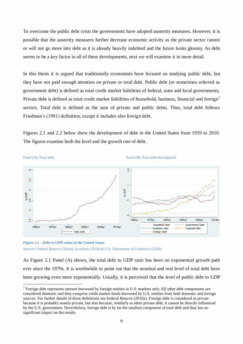
As the examples of Greece and Japan will demonstrate, the public debt to GDP ratio does not tell
the whole story. According to IMF (2011), Greece's public debt to GDP ratio is going to be
approximately 150 % until the end of 2011. As a consequence, the interest rate of Greece
government 10 year bonds has peaked at 26 % in September 2011, as Bloomberg (2011a) confirms.
Interestingly, IMF (2011) estimates the public debt to GDP ratio in Japan to be over 230 % in the
26
end of 2011. Nevertheless, according to Bloomberg (2011b), Japan pays only 1 % interest on its 10
year government bonds in September 2011. Actually, the interest rate of Japan government bonds
has been dropping for a long time, while the public debt to GDP ratio has been constantly
increasing. Why?
Typically, Japan's low interest rate has been explained by a high domestic saving rate and that Japan
is mainly indebted to its own citizens (see e.g. Reinhart and Rogoff 2010). According to Reinhart
and Rogoff (2010), foreign investors own the majority of Greece's (as well as other PIIGS8-
countries') debt. This is, undoubtedly, true but it does not reflect the fundamental causes. According
to Nersisyan and Wray (2010), it is highly unlikely that Japanese investors would ignore the risk
that the government of Japan might default on its debt obligations. They argue that Japanese
investors have all the chances to buy some other country's government bonds, instead of buying
government bonds of Japan.
According to Nersisyan and Wray (2010), a more fundamental cause for the low interest rate of
Japanese government bonds is that Japan has gotten into debt in its own currency, unlike Greece
and other Europe’s Economic and Monetary Union (EMU) member states. Nersisyan and Wray
(2010) argue that the central bank of a financially sovereign country9 can credit the government's
account without any limit. Thus, the government of a financially sovereign country can manage all
its debt obligations at any given time. In other words, the solvency of a financially sovereign
country can never be threatened.
Nersisyan and Wray (2010) insist that this is the case also with Japan. Government of Japan has its
own central bank, from where it can lend yens as much as it wants – at an interest rate it sets to
itself. Japan has borrowed yens and it is also the issuer of yens. Greece, on the other hand, has
mainly borrowed euros, but it is only the user of euros, not the issuer. Nersisyan and Wray (2010)
argue that, in this sense, Greece should be compared to a state in the United States and not consider
it as a financially sovereign country. Greece has not an own central bank, but shares one with all
EMU member states. In addition, in the EMU member states there exists no central fiscal authority,
who could borrow directly from the ECB, and look after the solvency of every member state.
Neither are there any mechanisms of income redistribution among the EMU member states.
8 Portugal, Ireland, Italy, Greece and Spain. 9 A country that has an independent fiscal and monetary policy with a floating exchange rate. In addition, the country
has not made any promises to exchange the currency to any commodity, for example, gold.
27
Consequently, Nersisyan and Wray (2010) argue that Japan's public spending is not income
constrained as is the case with Greece. Yet, the constraints are less restrictive if the country can run
current account surpluses to accumulate foreign currency – but this is neither the case with Greece.
Investors are aware of these facts that the solvency of the Japanese government can never
deteriorate, as opposed to the solvency of the Greece government. For this reason investors demand
a notably higher interest on Greece government bonds than Japanese government bonds.
The same argument can be taken even further with the United States. The United States is a
financially sovereign country. It could be said that the United States is actually the most sovereign
country in the world, if it would not have set a debt ceiling for itself, as the U.S. dollar is also
globally the most commonly used reserve currency. The United States pays, according to
Bloomberg (2011c), 2 % interest on its 10 year government bonds in September 2011, while IMF
(2011) estimates the public debt to GDP ratio to be 100 % in the end of 2011. Investors do not seem
to question the ability of the United States to clear all of its debt obligations as the interest rate of its
10 year government bonds has been constantly declining, as Bloomberg (2011c) confirms, even
though the debt ceiling was almost not raised on the 2nd
of August 2011 due to political
confrontations in the congress. Not raising the government debt ceiling would have pushed the
United States into insolvency.
As explained above, public debt can only artificially drive a financially sovereign country into
insolvency. The only “genuine” constraint, and which can also drive a country into insolvency, is
external debt. Reinhart and Rogoff (2009, 10) define external debt as debt “issued under another
country's jurisdiction, typically (but not always) denominated in a foreign currency, and typically
held mostly by foreign creditors.” Nersisyan and Wray (2010) define external debt10
as debt
denominated in a foreign currency. Consequently, they argue that it is irrelevant whether the
government bonds are owned by domestic citizens or foreigners. External debt is denominated in a
foreign currency and, thus, cannot be cleared simply by “printing money11
” as the exchange rate
would probably also be affected.
10 Notice that foreign debt defined in Chapter 2 is not comparable to external debt. In addition, all debts of Greece
government can be considered to be “external” in the sense that Greece cannot issue money in order to clear its
maturing debt obligations. 11 According to Kauko (2010), printing notes does not actually monetize outstanding domestic debt as notes are also
issued against debt. Notes, however, do not bear interest and they have an infinite maturity. Thus, printing notes only
changes the structure of debt, but not the amount. Only coins are not issued against debt and can be considered as debt-
free money.
28
Thus, Nersisyan and Wray (2010) admit that external debt can be very problematic. Also if the
currency is pegged into another currency or promised to exchange for some precious metal such as
gold, they argue that it can cause serious problems. However, Nersisyan and Wray (2010) point out
that domestic debt of a financially sovereign country does not set any operational constraints for the
government. They also argue that the need to balance the budget over some time period is a myth.
There are no financial constraints inherent in the fiat system that exist under a gold standard or
fixed exchange rate regime.
Reinhart and Rogoff (2009) make many rigorous remarks on financial crises in their book “This
Time Is Different” and finally ironically conclude that this time is actually not different. However,
Reinhart and Rogoff (2009) also argue that big public debt reduces economic growth due to
dampened confidence towards the country's repayment ability. They rely on Ricardian equivalence
theory as economic actors assume that ultimately taxes need to be raised and thus they spend less
today, which lowers the economic growth rate. This, in turn, forces the public sector to cut
spending, which will ultimately cause even more disturbance to economic growth.
As has been explained above, this conclusion does not seem to be in line with the modern money
theory, where a financially sovereign country does not face an income constraint for public
spending. For this reason, Nersisyan and Wray (2010) criticize Reinhart and Rogoff (2009) for
assuming too simply that correlation implies causality. If one simply takes average growth rates at
different levels of public debt, certainly there will be a negative correlation. Nersisyan and Wray
(2010) insist that causality runs the other way around: the income of the public sector tends to drop
in recessions, and for this reason the public sector ends up rapidly into heavy debt. In other words,
when the economic growth weakens, leads it to rising public debt – and not vice versa. They argue
that the current financial crisis is an excellent example of this link; it is not plausible to argue that
the financial crisis in the United States was due to too much government debt.
In defense for Reinhart and Rogoff (2009) it must be stated that their research covers past eight
centuries. During that period most countries were not financially sovereign as their currencies were
usually pegged to some precious metal or, at least, promised to exchange for another currency with
a fixed exchange rate. Consequently, it is possible that governments were, at least to some extent,
income constrained historically, but it does not imply that they still are in the modern world. Thus,
the conclusion of Reinhart and Rogoff (2009) can be as correct as Nersisyan and Wray’s (2010)
conclusion, but they depict different times in history.
29
3.4 Monetary circuit theory
This section describes the monetary circuit theory, or circuitism. As has been explained above, it is
a branch of the endogenous money creation theory. The monetary circuit theory focuses on how
production takes place from the perspective of money and debt. The first outlines of the monetary
circuit theory were given by Parquez (1984) and Lavoie (1987). However, first detailed analysis of
the theory was given by Graziani (1989). Other modern proponents of the circuitist approach are
Rochon (1999), Febrero (2006) and Keen (2009). This section mainly follows the circuit theory by
Graziani (2003), which is probably one of the most prominent works within the branch. First, a very
simplified version, which heavily relies on some underlying assumptions, is presented. Later, some
extensions are made to the model.
In mainstream economics money functions as a means of trade or as a stock of liquid wealth. In
neither case it is considered fundamental to the production process or the distribution of income.
Graziani (2003) challenges this view in his formulation of the monetary circuit theory.
Graziani (2003, 17) argues that circuitists hold that the role of money is to enable the circulation of
commodities, but it also determines the level of production and consumption. According to Graziani
(2003, 17-18), the term “monetary circuit” draws its origin from the fact that the theory studies the
complete life cycle of money: from its creation by the banking system, via its circulation in the
market, to its destruction at the time of repayment.
In principle, the monetary circuit theory accepts the chartalist view of money and, hence, should be
seen as complementary rather than an alternative. Yet, proponents of the circuit theory build models,
which typically have neither a government sector nor an explicit role for a central bank (see e.g.
Graziani 2003, 26-32). According to Keen (2009), the model does not need a central bank as long as
transfers between private bank accounts are accepted as making final settlement of debts between
buyers and sellers.
The fundamental insight of the circuit theory is that banks create money ex nihilo when granting
credit to creditworthy borrowers to make payments to third agents. Hence, all sales in a monetary
economy involve three parties: a seller, a buyer and a bank. The bank's role is to transfer a necessary
30
number of monetary units from the buyer's account to the seller's account. Next, the most simplified
model of the monetary circuit is presented.
Graziani (2003, 26-31) assumes that production takes time and it occurs in a closed market
economy. The model is as follows:
1. The monetary dynamics begin with a decision by banks to grant credit to firms.
2. This enables the firms to start a production process. With the borrowed money, the firms can
pay workers for producing commodities.
3. When the workers spend their income on the produced commodities, money is returned to
the firms.
4. Now, the firms can use this money to repay their debts to the banks.
As the issuance of debt creates money, similarly the repayment of debt destroys money. Thus,
according to Graziani (2003, 30), when the firms repay their debts to the banks, the circuit is closed.
As a result, the balance sheet of every economic actor is at its initial value, which is zero. However,
the temporary existence of bank credit created real economic transactions thus leaving the economy
better off than without the temporary credit extension.
The demand for and supply of credit is assumed to be mainly affected by future prospects
(including current indebtedness) to service and repay debt. For example, if a firm expects to make
enough profit from a potential investment after servicing and repaying the debt needed to finance
the investment, the firm will most likely demand credit. If also a bank evaluates that the firm is able
to carry out the payments related to the potential debt, the bank will most likely supply credit.
In the simple model described above the circuit closes only if some underlying assumptions are
satisfied. The model requires that the workers spend their incomes entirely on the goods and
services produced by the firms (including on purchases of corporate bonds). If they do not, then
some serious dilemmas arise. Graziani (2003, 30) argues that if the workers choose instead to keep
some portion of their income in the form of liquid balances, such as cash, and not spend it, firms are
unable to repay their debts to the banks. This typical behavior of the workers (and every economic
actor in order to prepare for uncertain future) is called “hoarding”. In order to avoid this dilemma, it
is suggested that the money supply must continuously increase to finance a constant scale of
production. According to Graziani (2003, 31), the money supply in the second circuit must equal the
wage bill of the workers plus the liquid balances put aside by the workers. Alternatively, Febrero
31
(2006) suggests that firms must negotiate with banks a conversion of short-term debt into long-term
debt.
Another dilemma, which many circuitists omit, is interest. Graziani (2003, 31) acknowledges this
and suggests that part of the commodities have to be sold to the bankers. This seems reasonable as
bankers can spend the interest payments back to the economy thus enabling full settling of debt. If
they do not spend the interest payments entirely, it is, in effect, exactly the same dilemma of
hoarding. In this case, the money supply in the second circuit to finance a constant scale of
production must equal the wage bill of the workers plus the liquid balances put aside by the workers
and bankers.
Graziani (2003, 32) identifies a further conundrum in his simple model: the money profits of the
firms are zero in the aggregate. This seems implausible as it can be shown that, in reality, the firms
can indeed make aggregate profits in a given time horizon. Due to this reason the circuitists have
sometimes been criticized for that the real world cannot possibly work in their theory. Keen (2009),
on the other hand, argues that these conundrums are due to applying wrong analytical tools to valid
economic insights. Keen (2009) models the circuit theory with a highly mathematical dynamic
model, which does not include either a government sector or a central bank. In his model of pure
credit economy firms can, besides making monetary profits in the aggregate, also service and repay
debt with a constant scale of production.
Another major shortcoming of the circuit theory is to undermine money creation for other purposes
than investments on production. As you have probably noticed, in the model above the banks do not
issue credit directly to the workers. Instead, workers have to acquire purchasing power indirectly
from the firms, who have exclusive access to credit. In reality, of course, banks grant credit also for
other purposes, such as private consumption and asset acquisition. Also this creates new purchasing
power, which can then circulate in the economy.
According to Febrero (2006), introducing additional economic actors and alternative circuits does
not radically alter the main message of the monetary circuit theory. He argues that it is possible to
add a government, a central bank and international trade into the model and stick to its implications.
He also argues that the implications are not affected even if households are granted access to credit
and if borrowing for speculative purposes is allowed. Febrero (2006) argues that including these
modifications does not alter the main message, although it can enrich the analysis. In the figure
32
below, a more comprehensive picture of the circuit theory is outlined. Notice that the figure is
author’s own view of the circuit theory and it is not necessarily fully in line with the perspectives of
other circuit theorists.
Figure 3.2 – An extension of the monetary circuit theory
Source: Author.
Figure 3.2 above presents a more complex process, where debt is created for a variety of purposes
in the economy. Debt creation is affected – besides other supply and demand factors – by two main
variables: interest rate and collateral rate. The reason why interest rate affects debt creation should
be obvious: it signals the price of acquiring additional purchasing power. The reason why collateral
rate affects debt creation was discussed in the first section of the present chapter.
In Figure 3.2 debt can be created for financing investment, private consumption and government
spending – all of which affect the real economy. This is illustrated by the red-blue arrow directing to
the left. The simple model described earlier captures only debt creation for investment purposes.
The feedback effects are represented by the curvy red-blue arrow. The logic behind this is that a
higher (lower) GDP might increase (decrease) debt creation as it enables more collateral to be used
even if the collateral rate stays unchanged. More collateral probably lowers the banks threshold to
grant credit at a given collateral rate.
In addition, debt creation can also be used for acquiring assets. As was discussed in Section 3.1,
debt creation for asset acquisition typically increases asset prices. Appreciated asset values can also
be used as collateral, which might induce debt creation similarly as a higher GDP. These
mechanisms are illustrated by the two red-violet arrows in Figure 3.2 above. Asset acquisition,
33
however, does not have any direct effects on the real economy. Yet, it can have indirect effects as
the purchasing power created for the asset markets might drift to the real economy. For example, a
firm can issue assets in order to invest in the real economy. Similarly, purchasing power can also
drift from the real economy to the asset markets. These mechanisms are illustrated by the two blue-
violet arrows.
It should be noted that, in Figure 3.2, money creation is already included into debt creation. This is
because of all money is debt12
. However, all debt is not money – at least in terms of typical money
supply measures such as M2 and M3.
Nevertheless, Figure 3.2 above does not capture the effects of hoarding. Hoarding simply implies
that all outstanding debt does not circulate in the real economy or in the asset markets (or in foreign
countries through imports or investments), but some purchasing power is put aside. Similarly,
dishoarding implies that more than observed change in debt affects the real economy or the asset
markets. Hoarding is analogous to Keynes’s liquidity preference, but here “liquid balances” cover
all debt instead of some money supply measure.
The rate of hoarding (or dishoarding) at any given time is affected by the liquidity preference of
economic actors. Typically the liquidity preference is assumed to depend on the distribution of
income and uncertainty of the future, among other factors. Distribution of income has an effect on
the aggregate liquidity preference, while the earners in the low-end tend to have a higher marginal
spending propensity than the earners in the high-end. Thus, hoarding has also macroeconomic
effects.
According to Moore (1988, 330), an increase in hoarding will lead to a decrease in the velocity of
circulation given the amount of debt and the share spend on asset markets. Consequently, if the
velocity of circulation is constant, it must indicate that hoarding by some agents must be offset by
dishoarding by some other agents. Therefore, if the velocity of circulation is constant, the aggregate
demand will remain unchanged.
Hoarding itself is assumed to be caused by the direct utility of money. For instance, money-in-the-
12 According to Kauko (2010), with the exception of coins, which are issued by the government and not by the central
bank, although the central bank typically buys them from the government. This, however, means that the government
does not have a liability in its balance sheet, but only central bank money (or coins in the case not selling them to the
central bank) as an asset.
34
utility-function (MIUF) models maintain that money yields utility not only when spent, but also
when kept idle. For instance, Fisher (1930, 215-216) and Keynes (1936) argue that people tend to
have liquid balances as a protection against uncertain future. According to King (1994), hoarding
increases especially during high level of debt. As economic actors tend to hoard and, consequently,
some other economic actors are unable to repay their debts, there is the risk of a debt deflation cycle
to emerge. Consequently, the aggregate demand is insufficient to satisfy the full production capacity
of the economy.
In order to avoid the problems of hoarding it has been suggested that the government can create
(monetary) net worth for the private sector. Nersisyan and Wray (2010) argue that when an
economic actor in the private sector goes into debt, its liabilities are another's assets. Thus, there is
no net worth creation. But when a financially sovereign country issues debt, it creates an asset for
the private sector without an offsetting private sector liability. According to Nersisyan and Wray
(2010), if the government is not income constrained, it can mitigate the problem of hoarding by
issuing debt through budget deficits. From this perspective, it seems peculiar that many
commentators defending the interests of either firms or tax payers insist that the governments
should cut their deficits in order to overcome the public debt crisis.
As the next chapter will reveal, this study will not try to model the whole complexity of the
monetary circuit. That would be by far too ambitious. Instead, this study will focus on the
relationship between debt creation and economic activity. Before presenting the model, the next
section will present some empirical studies, which are related to the theoretical factors outlined
previously in this chapter.
3.5 Related empirical studies
This final section of this chapter presents some selected empirical studies related to this thesis. The
studies presented here examine the relationship between quantity variables, such as money and debt
aggregates, and economic activity. The studies examine both the long run and the short run.
There has been a long-lasting dispute over (non-)neutrality of money. Neutrality of money indicates
that the level of money does not have any impact on the level of real economic activity,
unemployment or real interest rate, but only on the price level. Similarly, (super-)neutrality of
35
money implies that the growth rate of money does not have any effect on the growth rate of real
economic activity. Typically money is perceived non-neutral in the short run, but neutral in the long
run. First, we will go through studies examining the long-run effects and, then, we will examine the
short-run effects.
McCandless and Weber (1995) plot growth rates of real output and different money aggregates
against each other. The data is based on 1960–1990 and 110 countries. They find that money is
neutral in the whole sample as the slope is zero. However, they also find that in the subsample of
OECD countries there exists a positive correlation between money growth and real output growth.
Although this study has been taken as an evidence for long-run neutrality of money, money seems
to be non-neutral at least in the OECD subsample.
Bernanke (2000, 24), on the other hand, argues that during the Great Depression the effects of
monetary contraction on real economy were persistent and significant. He argues that to economists
it has been challenging to explain this persistent non-neutrality of money as typical models of non-
neutrality (such as those based on menu costs or money illusion) predict the effects to be only
transitory.
Friedman (1981) examines the relationship between nonfinancial domestic debt and economic
activity in the United States. He finds that the relationship has been very stable from 1946 to 1980,
although the public and private components of nonfinancial domestic debt have been unstable.
Friedman (1981) explains this either with crowding out effect or portfolio preferences. Crowding
out effect implies that increased budget deficits of the government crowd out private financing,
while portfolio preferences imply that, instead of crowding out, private sector shifts from debt to
equity financing. Nevertheless, it should be noted that even though the relationship between
nonfinancial domestic debt and economic activity was stable until 1980, according to Federal
Reserve (2010a), EconStats (2010) and U.S. Department of Commerce (2010), thereafter the ratio
has been growing almost constantly. Thus, expanding the sample until nowadays refutes Friedman’s
(1981) findings.
Next, we will go through some empirical studies examining the short-run effects. Conventionally,
fluctuations in money quantity used to contain information about future values of real income and
prices. Nowadays, it is typically perceived that this relation broke down in the late 1970s.
36
Sims (1972) studies the causality of money and income, which is measured with GNP. He uses
Granger causality tests with alternative lag specifications. Sims (1972) finds that money, measured
with the monetary base or M1 aggregate, is exogenous, but income is endogenous. That is,
fluctuations in money cannot be explained with the past fluctuations in income, but fluctuations in
income can be explained with the past fluctuations in money. In addition, he argues that the
temporal order of the variables does not necessarily imply causality, but it most likely does. Thus, it
is probable that changes in money are causing changes in income – and not vice versa.
Moore (1988, 307-308) estimates regressions for the relation between GNP growth and M3 growth
in the United States between 1959 and 1985. He uses both annual and quarterly data. He finds that
in annual data a lagged change in M3 explains about 70 % of the contemporaneous change in GNP,
while in quarterly data it explains approximately one third. Moore (1988, 308-311) also estimates
regressions for international comparison for total bank credit growth and GNP growth, and found
similar results.
Friedman and Kuttner (1992) estimate the following equation:
∆𝑦 = 𝛼 + ∑ 𝛽𝑖∆𝑚𝑡−𝑖4𝑖=1 + ∑ 𝛾𝑖∆𝑔𝑡−𝑖
4𝑖=1 + ∑ 𝛿𝑖∆𝑦𝑡−𝑖
4𝑖=1 + 𝑢𝑡 (3.3)
where y, m and g are all in natural logarithms and are, respectively, nominal or real income (defined
as GNP), financial variable and mid-expansion of federal expenditures. All data is quarterly and
seasonally adjusted. As a financial variable, Friedman and Kuttner (1992) use separately MB, M1,
M2 and credit, which includes the outstanding indebtedness of domestic nonfinancial borrowers.
The main finding of Friedman and Kuttner (1992) is that neither credit nor any of the money
aggregates are useful to predict nominal or real income after 1979, while before that they contained
significant predictive power. In addition, they find that market interest rates – especially the spread
between the interest rate on prime 4–6 month commercial paper and the 90-day Treasury bill –
contain significant information about the future fluctuations in nominal and real income.
Bernanke (2000, 58) estimates the following equation and obtains parameter values:
where 𝑌𝑡 is the rate of growth of industrial production relative to exponential trend and (𝑀 −𝑀𝑒)𝑡
is the rate of growth of nominal and seasonally adjusted M1 less predicted rate of growth. The data
is on a monthly level. Bernanke (2000, 58) finds that the first three explanatory terms are
statistically highly significant, but the last three terms before the error term are not significant even
at 10 % level. Thus, a contemporaneous deviation of M1 money aggregate from the expectation has
an effect on the contemporaneous industrial production.
Adrian et al. (2010) argue that there exists an inverse relation between macro risk premium and real
GDP growth. The higher the macro risk premium is the slower is the real GDP growth. As
methodology, they use standard vector autoregressive model and present impulse response
functions. Their study focuses mainly on the United States, but they also conduct an international
comparison including Germany, Japan and the United Kingdom. The results seem to be consistent
also internationally.
The next chapter presents the model and describes the key variables. Furthermore, three hypotheses
based on previous theoretical and empirical considerations are presented.
38
4 MODEL, DATA AND HYPOTHESES
This chapter presents the model, which will be estimated later, and describes the data. In addition,
three hypotheses are presented. The econometric methods applied in estimation can be found in
Appendix A.
4.1 Model
This first section presents a two-variable structural vector autoregressive (SVAR or structural VAR)
model with multiple lags. A two-variable model is presented as the empirical analysis is also
conducted with two variables. This section follows Enders (2004).
We can use matrix algebra to write a primitive bivariate system as:
𝐵𝑥𝑡 = 𝛤0 + 𝛤1𝑥𝑡−1 + 휀𝑡 (4.1)
where 𝐵 = [1 𝑏12𝑏21 1
], 𝑥𝑡 = [𝑦𝑡𝑧𝑡], 𝛤0 = [
𝑏10𝑏20
], 𝛤1 = [𝛾11 𝛾12𝛾21 𝛾22
], 휀𝑡 = [휀𝑦𝑡휀𝑧𝑡
].
Premultiplication by B–1
gives us the vector autoregressive (VAR) model in standard form:
𝑥𝑡 = 𝐴0 + 𝐴1𝑥𝑡−1 + 𝑒𝑡 (4.2)
where 𝐴0 = 𝐵−1𝛤0, 𝐴1 = 𝐵−1𝛤1, 𝑒𝑡 = 𝐵−1휀𝑡.
For notational purposes, we will define ai0 as element i of the vector A0, aij as the element in row i
and column j of matrix A1, and eit as the element i of the vector et. With this new notation, we can
rewrite the previous equation in matrix form:
[𝑦𝑡𝑧𝑡] = [
𝑎10𝑎20
] + [𝑎11 𝑎12𝑎21 𝑎22
] [𝑦𝑡−1𝑧𝑡−1
] + [𝑒1𝑡𝑒2𝑡
] (4.3)
Because of the feedback inherent in a VAR process, primitive systems, such as equation (4.1),
cannot be estimated directly. The reason is that zt is correlated with the error term εyt and that yt is
39
correlated with the error term εzt. Standard estimation methods require that the regressors are
uncorrelated with the error term. There is no such problem in the standard VAR model as the
dependent variables are expressed in terms of lagged variables.
However, some information might be recovered from the primitive system if it can be identified.
The primitive system is underidentified unless we are willing to impose a restriction on at least one
parameter. Imposing zero restrictions, and thus settling for the standard VAR form, may waste
important information.
Choleski decomposition offers one way to restrict a necessary amount of parameters. In Choleski
decomposition the lower triangular of matrix B in equation (4.1) is set to zero. In equation (4.1)
above it implies setting 𝑏21 = 0, which means that zt has a contemporaneous effect on yt, but yt
affects {zt} sequence only with a one-period lag. Thus, the ordering of the variables determines
which variable has also a contemporaneous effect on another variable. Choleski decomposition
results in an exactly identified system.
When we have applied Choleski decomposition, the premultiplication of the primitive equation
(4.1) by B–1
gives:
[𝑦𝑡𝑧𝑡] = [
𝑏10 − 𝑏12𝑏20𝑏20
] + [𝛾11 − 𝑏12𝛾21 𝛾12 − 𝑏12𝛾22
𝛾21 𝛾22] [𝑦𝑡−1𝑧𝑡−1
] + [휀𝑦𝑡 − 𝑏12휀𝑧𝑡
휀𝑧𝑡] (4.4)
When the system is estimated using ordinary least squares (OLS), the parameter estimates are from:
𝑥𝑡 = 𝐴0 + 𝐴1𝑥𝑡−1 + 𝑒𝑡 (4.5)
where 𝐴0 = [𝑎10𝑎20
] = [𝑏10 − 𝑏12𝑏20
𝑏20], 𝐴1 = [
𝑎11 𝑎12𝑎21 𝑎22
] = [𝛾11 − 𝑏12𝛾21 𝛾12 − 𝑏12𝛾22
𝛾21 𝛾22],
𝑒𝑡 = [𝑒1𝑡𝑒2𝑡
] = [휀𝑦𝑡 − 𝑏12휀𝑧𝑡
휀𝑧𝑡].
The variances and covariance are:
𝑉𝑎𝑟(𝑒1) = 𝜎𝑦2 + 𝑏12
2 𝜎𝑧2 (4.6)
𝑉𝑎𝑟(𝑒2) = 𝜎𝑧2 (4.7)
40
𝐶𝑜𝑣(𝑒1, 𝑒2) = −𝑏12𝜎𝑧2 (4.8)
We can generalize the previous structural VAR system in equation (4.5) to multiple lags case:
[𝑦𝑡𝑧𝑡] = [
𝑎10𝑎20
] + [𝑎11(1) 𝑎12(1)
𝑎21(1) 𝑎22(1)] [𝑦𝑡−1𝑧𝑡−1
] + (4.9)
+[𝑎11(2) 𝑎12(2)
𝑎21(2) 𝑎22(2)] [𝑦𝑡−2𝑧𝑡−2
] + ⋯+ [𝑎11(𝑝) 𝑎12(𝑝)
𝑎21(𝑝) 𝑎22(𝑝)] [𝑦𝑡−𝑝𝑧𝑡−𝑝
] + [𝑒1𝑡𝑒2𝑡
]
where aij(L) is the L-th lag of element in row i and column j of matrix AL, and p is the number of
lags.
The previous equation can also be written more compactly as:
𝑥𝑡 = 𝐴0 + ∑ 𝐴𝐿𝑥𝑡−𝐿𝑝𝐿=1 + 𝑒𝑡 (4.10)
Applying Choleski decomposition and including multiple lags we have the necessary tools for
estimating a structural VAR model. The model will be applied in the empirical analysis in the next
chapter.
4.2 Data description
The present section describes the key variables used in estimation and also explains the rationale
behind them. The theoretical framework outlined in Chapter 3 suggests studying the interactions
between money (or debt) aggregates and economic activity. As the monetary circuit theory implies,
monetized debt obligations (money supply measures) are a determinant of contemporaneous and
future economic activity, but they are also an outcome of past economic activity. In this study,
however, total debt and GDP are chosen as the main variables. They were chosen because of variety
of reasons, which are explained below.
Adrian and Shin (2009) argue that traditionally depository banks were the dominant suppliers of
credit, but their role has increasingly been replaced by market-based institutions, in particular those
involved in the securitization process. Consequently, Adrian and Shin (2009) suggest that there are
less reasons to study typical bank-based credit, that is, typical money supply measures such as M2
41
and M3. Adrian and Shin (2011) argue that the traditional money supply measures were valid
instruments before the market-based financial system, but not after that. The reason why they argue
so is probably that the money supply measures are not comprehensive enough to measure the
aggregate purchasing power of the economy and, thus, they do not have any relevant meaning.
In fact, Adrian and Shin (2010) define aggregate liquidity through the aggregate balance sheet of
financial institutions (including, for example, depository banks, investment banks, insurance
companies and pension funds). Adrian and Shin (2011) suggest that balance sheet quantities of
financial institutions, such as total assets or leverage, could be more modern counterparts for
traditional money supply measures. They argue that, ironically, quantity aggregates – although not
traditional money quantity measures – have made a return into monetary policy analysis after a long
period of silence, which Friedman and Kuttner (1992) among others put forward.
Adrian and Shin (2011, 65) argue that the “money stock is a measure of liabilities of deposit-taking
banks, and so may have been useful before the advent of the market-based financial system.” Their
argument supports measuring the aggregate liquidity in the economy with a more comprehensive
measure than only measuring liabilities of deposit-taking banks. This is also in line with Minsky
(1982 & 1986) as he argues that, in a regulated market, increased demand for and supply of debt
manifest themselves through market-based financial institutions, which do not affect the money
supply measures.
But why should we limit our scope to cover only the balance sheets of financial institutions
(including deposit-taking banks)? Any economic actor can issue credit and, in a highly liquid world,
it can be sold in the market. In addition, when any debt is created, very likely a market transaction is
also created at the same time or briefly afterwards. Otherwise, there would be no point to demand
for purchasing power and repay it with interest. Thus, it is argued that the total debt of all (domestic
and foreign) economic actors borrowed from domestic sources is a much better measure of
aggregate purchasing power in the economy. This is the reason why the present study has chosen to
examine total debt instead of the traditional money supply measures or the aggregate balance sheet
of financial institutions. Figure 4.1 below depicts the vast difference between total debt and
traditional money supply measures.
42
Figure 4.1 – Money aggregates and total debt
Sources: Federal Reserve (2010a & 2010b) & EconStats (2010).
Note: Federal Reserve ceased publishing M3 statistics in March 2006.
As Figure 4.1 above illustrates, total debt is notably larger than any of the typical money
aggregates. It is argued in the spirit of Adrian and Shin that total debt can capture credit creation of
market-based institutions, but also other credit creation. Hence, total debt is the comprehensive
measure of the aggregate purchasing power of the economy.
Money supply measures could be included into the analysis as a third endogenous variable.
However, in this case it should be deducted from total debt. Decomposing total debt into monetized
debt and non-monetized debt and studying their different impacts might be interesting. Instead of
money supply measures, aggregate balance sheet of financial institutions could also be used.
Nevertheless, this thesis will focus on different aspects.
All debt, however, does not affect the domestic economic activity. The debt of foreign entities
borrowed from domestic entities should be included into the analysis as it probably mainly affects
exports and, thus, has an influence on the GDP. However, the debt of domestic entities borrowed
from foreign entities should be excluded from the analysis as it is probably used to finance imports,
which are not part of the GDP. For example, the federal debt of the United States borrowed from
China should be excluded from the analysis as it is likely to affect mainly the imports of the United
States. Thus, external debt, defined by Reinhart and Rogoff (2009, 10), should be excluded from the
analysis. Reinhart and Rogoff’s (2009, 10) definition of external debt might be inappropriate for
explaining the modern money theory, but it seems to be appropriate for analyzing the interaction
between debt and economic activity.
43
Unfortunately, Federal Reserve (2010a) and EconStats (2010) register external debt under domestic
debt. That is, they do not provide data on whether domestic debtors have borrowed from domestic
or foreign sources. On the other hand, they provide numbers for foreign debt, which is defined as
debt of foreign entities borrowed from the U.S. credit markets. Therefore, as has been argued above,
foreign debt can have an effect on the GDP of the United States as it probably affects the export
sector and, hence, should be included into the analysis.
The choice of variables can be seen as complementary to Geanakoplos’s (2010) theory of the
leverage cycle. We argue that a change in total debt captures how leverage is actually utilized. It is
possible that even during very low collateral rates debt is, for some reason or another, not issued.
Thus, asset prices do not go up, even if huge leverage would be possible. One factor that might
neutralize the possibility to leverage aggressively could be a high interest rate. High interest rate
might suspend the eagerness to buy with borrowed money. Thus, it is argued that total debt change
is actually the realization of these two factors (interest rate and collateral rate), future prospects and
possibly some other factors too. Therefore, total debt change could be used as a variable to explain
changes in asset prices.
Nevertheless, this study is more interested in the real economy. There is no reason why leverage,
and thus total debt, could not push the demand up also in the real economy. For these reasons, this
thesis replaces asset prices used in Geanakoplos’s (2010) study with economic activity and
collateral rate with total debt. However, it would be pretty straightforward to limit our study to only
nominal variables as it is very probable that an increase in nominal total debt really does push the
nominal GDP up – either by inflation or by increased output. In order to cope this, the variables are
studied also in real terms.
According to Fisher (1933), debt and deflation are the fundamental causes of disturbances in almost
all other economic variables. Treating the variables in real terms removes the price level from the
analysis as an independent factor. In other words, the price level is already included in total debt
and GDP, when they are measured in real terms. For example, deflation can cause a stampede to
repay debt and, therefore, the real value of debt changes causing also a change in real economic
activity. When the variables are in real terms, the price level effects are included in the variables
and, thus, there is no need to include the price level separately into the analysis.
Now the rationale behind the choice of the variables has been explained. Next the data collection
44
process and its modifying procedures are described.
The data is based on the United States macro level statistics and it is a time series organized
quarterly from 1959 first quarter to 2010 first quarter. This time horizon is chosen because it is the
longest possible time horizon, where data on all the variables is available. None of the variables is
originally seasonally adjusted.
The time series is not perfectly balanced. Some variables have missing values in the end due to the
lag in collecting statistics. The consumer price index (CPI), which is obtained from U.S.
Department of Labor (2010), has been converted from monthly to quarterly by taking arithmetic
average from the corresponding months of every quarter. As a base value the CPI uses the average
of 1982–1984 prices. All other data is originally quarterly.
The variables are converted to seasonally adjusted logarithmic differences, which approximates the
annual rate of change. First, nominal GDP is collected from U.S. Department of Commerce (2010)
and nominal total debt is obtained from Federal Reserve (2010a) and EconStats (2010). As has been
explained in Chapter 2, total debt is the sum of household debt, business debt, financial debt,
foreign debt, federal government debt, state government debt and local government debt. Foreign
debt has already been defined in Chapter 2 (for detailed definitions of other debt components see
Federal Reserve 2010a). Thus, both nominal variables are originally reported quarterly. They are
converted into real terms by dividing the nominal variable with the CPI.
The variables in nominal and real terms are then transformed into logarithmic form by taking a
natural logarithm. Logarithmic form is applied in order to even out the variance depending on the
time of origin. Then, seasonally adjusted logarithmic difference is obtained by taking a difference
from the corresponding quarter of the previous year. Seasonal adjustment is used to remove the
seasonal variation, which is typical for quarterly data, from the variables. Otherwise, the estimation
results might not be fully reliable. Finally, the seasonally adjusted logarithmic differences are
converted into percentages by multiplying the variables by 100. In this study growth rate is
commonly used to refer to seasonally adjusted logarithmic difference. A summary of the variables is
presented in Table 4.1 below.
45
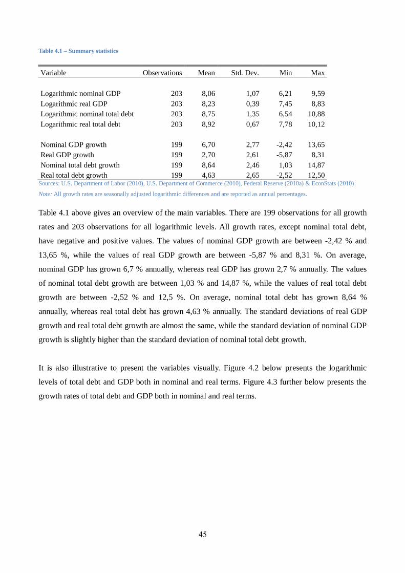
Table 4.1 – Summary statistics
Variable Observations Mean Std. Dev. Min Max
Logarithmic nominal GDP 203 8,06 1,07 6,21 9,59
Logarithmic real GDP 203 8,23 0,39 7,45 8,83
Logarithmic nominal total debt 203 8,75 1,35 6,54 10,88
Logarithmic real total debt 203 8,92 0,67 7,78 10,12
Nominal GDP growth 199 6,70 2,77 -2,42 13,65
Real GDP growth 199 2,70 2,61 -5,87 8,31
Nominal total debt growth 199 8,64 2,46 1,03 14,87
Real total debt growth 199 4,63 2,65 -2,52 12,50 Sources: U.S. Department of Labor (2010), U.S. Department of Commerce (2010), Federal Reserve (2010a) & EconStats (2010).
Note: All growth rates are seasonally adjusted logarithmic differences and are reported as annual percentages.
Table 4.1 above gives an overview of the main variables. There are 199 observations for all growth
rates and 203 observations for all logarithmic levels. All growth rates, except nominal total debt,
have negative and positive values. The values of nominal GDP growth are between -2,42 % and
13,65 %, while the values of real GDP growth are between -5,87 % and 8,31 %. On average,
nominal GDP has grown 6,7 % annually, whereas real GDP has grown 2,7 % annually. The values
of nominal total debt growth are between 1,03 % and 14,87 %, while the values of real total debt
growth are between -2,52 % and 12,5 %. On average, nominal total debt has grown 8,64 %
annually, whereas real total debt has grown 4,63 % annually. The standard deviations of real GDP
growth and real total debt growth are almost the same, while the standard deviation of nominal GDP
growth is slightly higher than the standard deviation of nominal total debt growth.
It is also illustrative to present the variables visually. Figure 4.2 below presents the logarithmic
levels of total debt and GDP both in nominal and real terms. Figure 4.3 further below presents the
growth rates of total debt and GDP both in nominal and real terms.
46
Panel (A): Nominal Panel (B): Real
Figure 4.2 – Logarithmic levels of total debt and GDP
Panel (A): Nominal Panel (B): Real
Figure 4.3 – Growth rates of total debt and GDP
Note: All growth rates are seasonally adjusted logarithmic differences.
4.3 Hypotheses
This section presents three hypotheses, which are motivated by the following questions. Does total
debt affect GDP? Does GDP affect total debt? If either one does, what are the effects? Can we say
anything about the causality?
The theoretical framework and related studies discussed in Chapter 3 might provide some answers.
However, these answers should also be tested empirically. According to the theoretical framework,
47
following hypotheses have been constructed:
Hypothesis 1: Contemporaneous and past total debt affects contemporaneous GDP. In other
words, the hypothesis suggests that GDP is endogenous. This is assumed to be due to
contemporaneous and past total debt might determine production, consumption and public
spending possibilities.
Hypothesis 2: Past GDP affects contemporaneous total debt. In other words, the hypothesis
suggests that total debt is endogenous. This is assumed to be due to the possibility that past
GDP might be used as collateral for debt creation.
Hypothesis 3: GDP growth responds differently to a shock in total debt growth depending on
the time horizon. High (low) total debt growth might increase (decrease) GDP in the near
future, but it might decrease (increase) GDP in the distant future. This is supposed to be due
to changes in purchasing power and inflexible prices. Total debt growth might increase
economic activity in the near future as more purchasing power is created than returned. In
contrast, total debt growth might decrease economic activity in the distant future as more
purchasing power is returned than created as debts mature. In addition, hoarding
(precautionary saving) might be more common during high level of debt.
The three hypotheses above will be empirically tested in the next chapter.
48
5 ECONOMETRIC ANALYSIS
This chapter presents the preliminary tests, the estimated regressions and the postestimation results.
First, however, some illustrative figures are presented and interpreted. Second, stationarity is tested.
Third, cointegration is tested. Fourth, the estimated regressions are presented. Fifth, Granger
causality is tested. Sixth, impulse response functions are visually presented. Finally, forecast error
variance decompositions are also visually presented. A detailed description of the applied
econometric methods can be found in Appendix A.
The present chapter examines the dynamic effects of total debt and GDP. The theory discussed in
Chapter 3 suggests studying the relation between debt and GDP. Previous studies, such as Sims
(1972), Moore (1989) and Bernanke (2000), use two-variable systems in order to explain the
interactions between money (or debt) aggregates and economic activity. In addition, Minsky (1982
& 1986) and Adrian and Shin (2009 & 2011) argue that instead of the money supply measures more
comprehensive credit aggregates should be analyzed. Moreover, any debt creation will most likely
be followed by a market transaction due to logical reasons. All these factors support the choice to
use two-variable structural VAR model in order to study the dynamic interactions of total debt and
GDP.
5.1 Total debt and GDP at a glance
This section examines the interrelations between total debt and GDP simply by presenting some
illustrative figures. The figures can also be helpful when determining the correct specification of the
model to be estimated. First, the contemporaneous effects are briefly examined. Then, we will move
to examine the dynamic effects.
A very rough way of examining the existence of a relationship between total debt and GDP is to
plot them against each other. Figure 5.1 shows the growth rates of total debt and GDP against each
other.
49
Panel (A): Nominal growth rates Panel (B): Real growth rates
Figure 5.1 – Scatterplots for total debt and GDP
Note: All variables are seasonally adjusted logarithmic differences.
As Figure 5.1 above depicts, there is a positive relation between the contemporaneous nominal and
real growth rates of total debt and GDP in the United States between 1959 and 2010. However, the
relation does not seem to be completely linear at least with the real growth rates. That is, even
though real total debt would grow faster, real GDP will not grow faster after a certain limit. The
limit seems to be approximately 8 % for both variables. This makes sense since real economy
clearly cannot grow arbitrarily fast and, thus, further real total debt growth would only stimulate
inflation instead of the real economy. On the other hand, negative real total debt growth can imply
deflation. Deflation, as has been discussed in Section 3.1, is known to be harmful for real economic
growth. Figure 5.1 Panel (B) shows that negative growth rates of real total debt are closely
associated with negative growth rates of real GDP.
There seems to be a positive contemporaneous correlation between the growth rates of total debt
and GDP, but it is even more important to study the dynamic effects. Figure 5.2 below presents the
time series of the real growth rates of total debt and GDP in the United States from 1959 to 2010.
As Figure 5.2 below confirms, real total debt and real GDP are clearly positively correlated. In other
words, real total debt is procyclical. As discussed in Chapter 3, creating new debt might increase
(decrease) GDP through new (lost) investment, consumption and public spending. The rate, at
which total debt is created (destroyed), is supposed to increase (decrease) as a consequence when
the central bank lowers (raises) the interest rate. However, an increase (decline) in GDP might also
enable more (less) debt creation as the collateral, against which debt is issued, increases (decreases).
50
Figure 5.2 – Real growth rates of total debt and GDP
Notes: Both variables are seasonally adjusted logarithmic differences and have been smoothed with
moving-average filter with four lags, one contemporaneous term and four forwards. The figure is
otherwise the same as Figure 4.3 Panel (B).
Interestingly, Figure 5.2 above depicts that real total debt has grown almost constantly faster than
real GDP after the year 1979, while before that they both grew approximately at the same rate. This
might be due to the new monetary policy procedures announced by the Federal Reserve in October
1979, which gave a start for an era of deregulation. This might also be deemed as Adrian and Shin’s
(2009 & 2011) turning point from bank-based credit to market-based credit.
The fact that real total debt has grown faster than real GDP might have some interesting
implications. It might imply that new purchasing power created by new total debt has mainly been
channeled to asset markets, instead of the real economy. This view is also supported by the fact that
asset prices, such as stock values, have grown notably faster than the real economy from 1979
onwards. If the new purchasing power would have been channeled solely to the real economy, the
total debt to GDP ratio could not have changed (unless the velocity of circulation changes), that is,
their growth rates should not depart from each other. Why? There are three explanations. First, if
new purchasing power would create real economic growth exactly in the same proportion, the ratio
could not change. Second, if new purchasing power would be only inflationary without any real
economic effects, the ratio could not change either as inflation is removed from the variables. Third,
logically a combination of these two effects should neither have any effects on the ratio. As the total
debt to GDP ratio has changed, as Figure 2.1 Panel (A) illustrated, we can relatively safely conclude
that new purchasing power created by an increase in total debt after 1979 has mainly been
channeled outside the real economy.
51
The structural break in 1979, however, should not go unnoticed in the regression analysis as it could
affect the estimates differently during these two periods. The existence of a structural break implies
two possible adjustments. Either a dummy-variable should be added from 1979Q4 onwards (or until
1979Q3). This might be the point when Adrian and Shin’s (2011, 65) “market-based financial
system” replaced its predecessor. Alternatively, two separate regressions could be estimated for pre-
and post-1979.
These procedures are commonly used in other empirical studies, where interactions between
quantity measures and economic activity are estimated. For instance, Friedman and Kuttner (1992)
use both methods. They adapt the third quarter of 1979 as a threshold for one subsample because
the Federal Reserve introduced its new monetary policy procedures in October 1979.
Next, we will take a brief outlook at the autocorrelations of the variables. Figure 5.3 presents the
autocorrelations of nominal variables, while Figure 5.4 presents the autocorrelations of real
variables.
Panel (A): Nominal GDP growth Panel (B): Nominal total debt growth
Figure 5.3 – Autocorrelations of nominal variables
Notes: Both variables are seasonally adjusted logarithmic differences. Bartlett's formula for MA(q) 95% confidence bands.
As Figure 5.3 above shows, both nominal variables are strongly and positively autocorrelated. The
first eleven lags of nominal GDP and the first nine lags of nominal total debt are statistically
significant. The autocorrelation of nominal GDP decays relatively rapidly to around 0,4 but
thereafter it is very persistent. The autocorrelation of nominal total debt, on the other hand, decays
very slowly and smoothly. Both variables seem to converge very slowly towards zero.
52
Panel (A): Real GDP growth Panel (B): Real total debt growth
Figure 5.4 – Autocorrelations of real variables
Notes: Both variables are seasonally adjusted logarithmic differences. Bartlett's formula for MA(q) 95% confidence bands.
According to Figure 5.4 above, also real variables are autocorrelated. However, only the first three
lags of real GDP and the first six lags of real total debt are statistically significant. Now, the
autocorrelation of real GDP decays notably fast to zero after five lags and then fluctuates around it.
The autocorrelation of real total debt decays more slowly reaching persistent negative values after
the tenth lag. Nevertheless, both variables tend to converge slowly towards zero.
Below in Figure 5.5 are shown cross-correlations between total debt growth and GDP growth. The
variables are both in nominal and real terms. Notice that total debt is on the horizontal axis
including lags and forwards, while GDP is on the vertical axis including only the contemporaneous
effects. Nevertheless, there is no reason to illustrate the variables with inverted axis because the
figure would simply be a mirror image (the cross-correlation of p-th lag of total debt with
contemporaneous GDP would be the same as the cross-correlation of p-th forward of GDP with
contemporaneous total debt).
According to nominal cross-correlations presented in Figure 5.5 Panel (A) below, there seems to be
a positive correlation between the nominal growth rates of GDP and total debt with all lags and
forwards. Correlation of the contemporaneous periods is the strongest correlation. The forwards of
total debt are also strongly correlated with GDP, while the lags are somewhat weaker correlated.
53
Panel (A): Nominal growth rates Panel (B): Real growth rates
Figure 5.5 – Cross-correlations of total debt and GDP
Notes: All variables are seasonally adjusted logarithmic differences. Total debt is on the horizontal axis (lags and forwards) and GDP
is on the vertical axis.
The argument that GDP is used as collateral for debt creation is supported by the fact that forwards
of total debt are strongly correlated with contemporaneous GDP. In addition, future GDP obviously
cannot be used as collateral, which could explain why lagged total debt is correlated weakly with
contemporaneous GDP. On the other hand, lagged total debt being weakly correlated with
contemporaneous GDP could indicate that past debt creation causing present GDP should be
questioned. However, the possibility that only the contemporaneous periods matter cannot be ruled
out. It is possible that contemporaneous total debt could cause contemporaneous GDP, even though
the lags of total debt do not have any effect on contemporaneous GDP.
When examining the real variables, as Figure 5.5 Panel (B) shows, the cross-correlations are
somewhat different. Still, the contemporaneous periods are most strongly and positively correlated.
Surprisingly, however, now the distant (more than 6 quarters) lags and forwards are negatively
correlated. Again the distant lags of real total debt are less correlated with contemporaneous real
GDP than distant forwards, but only slightly. The near (up to 6 quarters) lags and forwards are still
positively correlated. Now, however, the correlations of near lags and forwards are evenly
distributed, that is, the cross-correlations are not skewed. In addition, the cross-correlations of the
most distant lags and forwards tend to converge to zero.
The distant lags and forwards of real total debt being negatively correlated with contemporaneous
GDP raises some interesting questions. Could aggressive debt creation in the distant past affect
present GDP negatively? According to Figure 5.5 Panel (B), it might be possible. This makes sense
54
since, ceteris paribus, when past debts are repaid, more purchasing power is destroyed than created
(total debt is shrinking), which can affect contemporaneous real economic activity negatively if
prices are inflexible. Actually, this is analogous to the debt deflation theory, although the effect is
mitigated if new debt is issued in order to replace the repaid debts. This is also in line with King’s
(1994) observation that previous changes in private debt are negatively correlated with
contemporaneous changes in GDP in the 1990s recession. From this perspective, a higher (lower)
total debt growth rate could provide a higher (lower) GDP growth rate in the short run, but a lower
(higher) GDP growth rate in the intermediate run. The idea is captured by hypothesis 3, which was
already presented in Section 4.3.
What about future expectations? The interpretation of cross-correlations of the real variables is
consistent with the rational expectations theory (meaning that expectations will be realized in the
future). Thus, if a higher debt growth rate is expected in the near future, present real GDP increases.
The present real GDP is financed with increased present borrowing as the debt is easier to repay in
the future if there is going to be more borrowing in the future. In addition, it is reasonable to borrow
for investment or consumption if the interest rate is expected to drop soon (remember that the
central bank interest rate is assumed to influence the growth rate of total debt). However, if a lower
interest rate is expected to take place in the distant future, it is reasonable to wait and borrow later.
Consequently, the present GDP may be negatively affected. Again, it is possible to identify a
positive short-run relation, but a negative intermediate-run relation.
If we examine the most distant lags and forwards, the cross-correlations converge to zero.
Intuitively, it is easy to understand: very distant events in the past or future do not affect current
decision making. In other words, there are no long-run effects. Thus, the time horizon in the model
should be relevant. In the next section we will test the stationarity of the variables.
5.2 Stationarity tests
As Appendix A explains, a time-series analysis should begin with stationarity tests. Thus, this
section presents the results of the augmented Dickey-Fuller (ADF) tests. The tested variables are
logarithmic levels and growth rates (seasonally adjusted logarithmic differences) of total debt and
GDP both in nominal and real terms.
55
The variables were not tested in the level or difference form without first taking a natural logarithm
as they are clearly not stationary. In the level form both variables have an increasing mean and
variance in time and thus cannot be stationary. In the difference form both variables have a
relatively stable mean, but the variance is clearly increasing in time.
Table 5.1 below presents the ADF-tests for logarithmic levels and growth rates. The lag number for
every variable is determined using Akaike (AIC) and Bayesian (BIC) information criterion.
Table 5.1 – Augmented Dickey-Fuller tests
Variable Lags Test statistic Probability Stationary
Logarithmic nominal GDP 2 (BIC) -2,538 0,1064 No
Logarithmic nominal GDP 17 (AIC) -2,756 0,0648 Yes, P>90 %
Logarithmic nominal total debt 3 (BIC) -1,364 0,5992 No
Logarithmic nominal total debt 12 (AIC) -1,526 0,5206 No
Logarithmic real GDP 2 (BIC) -2,021 0,2773 No
Logarithmic real GDP 18 (AIC) -2,021 0,2773 No
Logarithmic real total debt 5 (BIC) -0,363 0,9162 No
Logarithmic real total debt 7 (AIC) -0,196 0,9390 No
Nominal GDP growth 13 (BIC) -1,084 0,7213 No
Nominal GDP growth 30 (AIC) -0,419 0,9069 No
Nominal total debt growth 9 (BIC) -1,349 0,6066 No
Nominal total debt growth 17 (AIC) -1,215 0,6670 No
Real GDP growth 14 (BIC) -3,468 0,0088 Yes, P>99 %
Real GDP growth 14 (AIC) -3,468 0,0088 Yes, P>99 %
Real total debt growth 9 (BIC) -3,412 0,0106 Yes, P>95 %
Real total debt growth 10 (AIC) -3,289 0,0154 Yes, P>95 % Notes: All growth rates are seasonally adjusted logarithmic differences. The information criterion supporting the lag choice is in the
parenthesis after the lag number. The ADF-test is conducted as a pure random walk model and thus does not include a drift term or a
linear time trend.
As Table 5.1 above shows, logarithmic GDP and total debt are nonstationary both in nominal and
real terms. This result should not come as a surprise as Figure 4.2 illustrates that the variables in
logarithmic levels clearly have an increasing mean in time, even though the variance seems
relatively stable. The only exception in logarithmic levels is the nominal GDP, when tested with 17
lags. In this case it is statistically significant at 10 % level, but not if it is tested with 2 lags. Hence,
using barely stationary logarithmic nominal GDP could be a risky and questionable choice.
56
Table 5.1 also shows that the nominal growth rates of the variables are not even remotely stationary.
This result is somewhat surprising as Figure 4.3 Panel (A) depicts that the mean wanders only
slightly across time and the variance is relatively stable. As Table 5.1 displays, the real growth rates
of the variables are, however, statistically significant at least at 5 % level. In other words, the real
growth rates of the variables are difference stationary I(1). Thus, it is reasonably safe to estimate the
model using real growth rates of total debt and GDP.
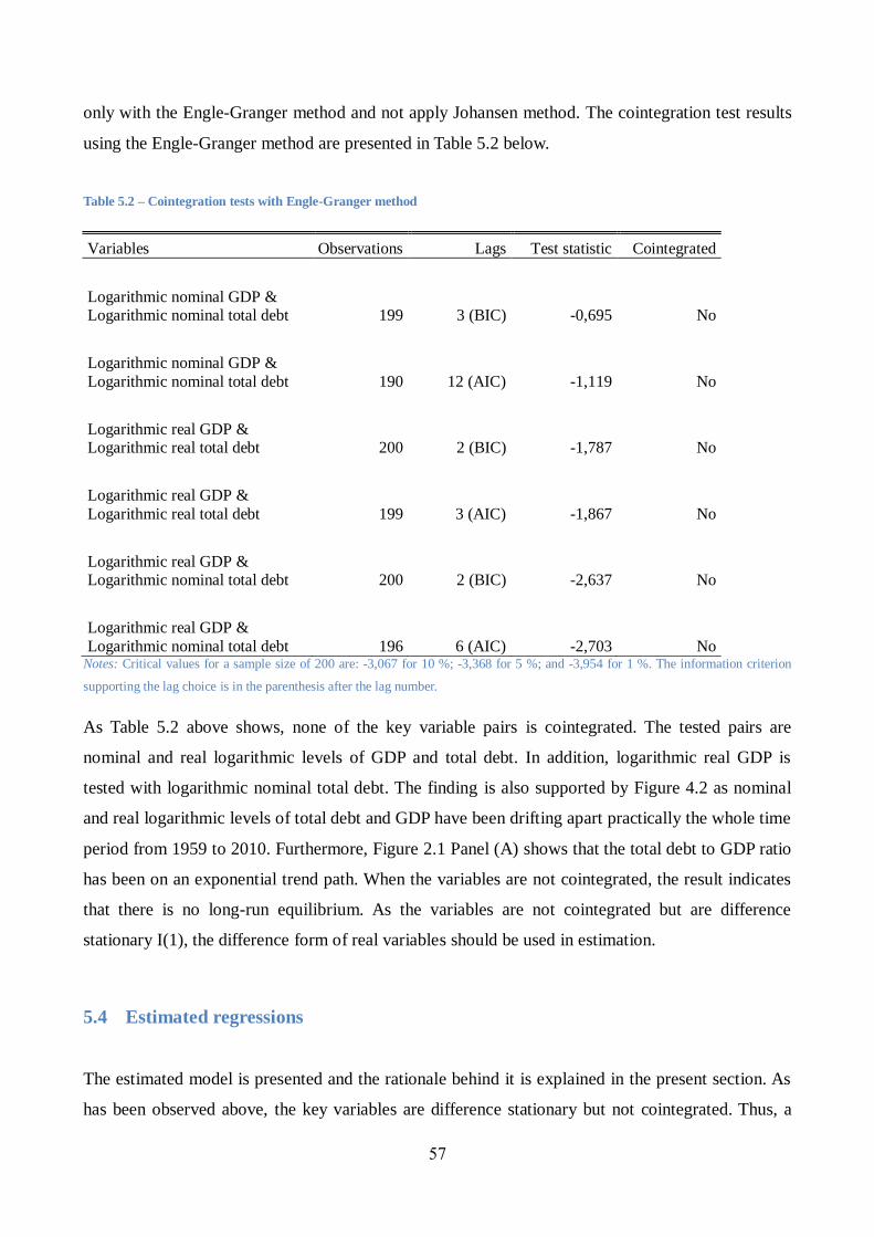
5.3 Cointegration tests
As concluded in the previous section above, the real growth rates of the variables are stationary.
Consequently, the variables cannot be straightforwardly estimated in the level form. Thus, the long-
run equilibrium13
between the variables cannot be studied, unless they are cointegrated. In the
present section cointegration of total debt and GDP is tested.
The economic logic behind the cointegration analysis is that economic variables do not typically
drift too far away from each other due to market mechanism or government intervention. This,
however, does not seem to be the case with the variables concerned in this study. As Figure 4.2
illustrated, it seems that real and nominal logarithmic levels of total debt and GDP have been
drifting apart practically the whole time period from 1959 to 2010. Thus, it seems unlikely that the
variables are cointegrated – at least in the time horizon examined in this study.
Nevertheless, the variables might be cointegrated in the very long run as, according to Morgan
Stanley (2009), the total debt to GDP ratio grew exponentially and reached 300 % in 1933, and
halved relatively fast in the next 10 odd years. As Figure 2.1 Panel (A) showed, the ratio climbed
again exponentially almost to 400 % until 2009, and thereafter it shows some signs of reaching a
turning point. Thus, it is possible that the total debt to GDP ratio will be dropping in the upcoming
years and, consequently, show some evidence of cointegration. Nevertheless, the potential
adjustment period is so long that it cannot be examined in this study.
As it seems unlikely that the variables would be cointegrated, we will settle to test for cointegration
13 It should be noted that econometricians typically have a different interpretation for the term equilibrium than
economists. These two interpretations should not be confused with each other. Here equilibrium simply refers to any
long-run relationship between non-stationary variables.
57
only with the Engle-Granger method and not apply Johansen method. The cointegration test results
using the Engle-Granger method are presented in Table 5.2 below.
Table 5.2 – Cointegration tests with Engle-Granger method
Variables Observations Lags Test statistic Cointegrated
Logarithmic nominal GDP & Logarithmic nominal total debt 199 3 (BIC) -0,695 No
Logarithmic nominal GDP &
Logarithmic nominal total debt 190 12 (AIC) -1,119 No
Logarithmic real GDP & Logarithmic real total debt 200 2 (BIC) -1,787 No
Logarithmic real GDP &
Logarithmic real total debt 199 3 (AIC) -1,867 No
Logarithmic real GDP & Logarithmic nominal total debt 200 2 (BIC) -2,637 No
Logarithmic real GDP &
Logarithmic nominal total debt 196 6 (AIC) -2,703 No Notes: Critical values for a sample size of 200 are: -3,067 for 10 %; -3,368 for 5 %; and -3,954 for 1 %. The information criterion
supporting the lag choice is in the parenthesis after the lag number.
As Table 5.2 above shows, none of the key variable pairs is cointegrated. The tested pairs are
nominal and real logarithmic levels of GDP and total debt. In addition, logarithmic real GDP is
tested with logarithmic nominal total debt. The finding is also supported by Figure 4.2 as nominal
and real logarithmic levels of total debt and GDP have been drifting apart practically the whole time
period from 1959 to 2010. Furthermore, Figure 2.1 Panel (A) shows that the total debt to GDP ratio
has been on an exponential trend path. When the variables are not cointegrated, the result indicates
that there is no long-run equilibrium. As the variables are not cointegrated but are difference
stationary I(1), the difference form of real variables should be used in estimation.
5.4 Estimated regressions
The estimated model is presented and the rationale behind it is explained in the present section. As
has been observed above, the key variables are difference stationary but not cointegrated. Thus, a
58
structural vector autoregressive (SVAR or structural VAR) model should be estimated in differenced
form for real total debt and real GDP.
In this study a structural VAR model is estimated using OLS. The model is the same as in equation
(4.9), or in a more compact form in equation (4.10). The estimated model presented already in
equation (4.9) is:
[𝑦𝑡𝑧𝑡] = [
𝑎10𝑎20
] + [𝑎11(1) 𝑎12(1)
𝑎21(1) 𝑎22(1)] [𝑦𝑡−1𝑧𝑡−1
] + (5.1)
+ [𝑎11(2) 𝑎12(2)
𝑎21(2) 𝑎22(2)] [𝑦𝑡−2𝑧𝑡−2
] + ⋯+ [𝑎11(𝑝) 𝑎12(𝑝)
𝑎21(𝑝) 𝑎22(𝑝)] [𝑦𝑡−𝑝𝑧𝑡−𝑝
] + [𝑒1𝑡𝑒2𝑡
]
where 𝑦𝑡 is seasonally adjusted logarithmic difference of real GDP, 𝑧𝑡 is seasonally adjusted
logarithmic difference of real total debt, and p is the number of lags. The number of lags is
determined with AIC and BIC, which suggest using 16 and 2 lags respectively.
As has been explained in Chapter 3, the contemporaneous causality runs from total debt to GDP.
The monetary circuit theory argues that debt creation is an important determinant of the production
process and hence must take place first. Thus, the variables have been ordered in this way and not in
the alternative way. In this ordering real total debt growth has a contemporaneous effect on real
GDP growth, but real GDP growth affects real total debt only with delay.
As explained in Section 5.1, due to the structural break in October 1979 the model is estimated
separately for the whole sample and two subsamples. The time horizon of the whole sample is
1959Q1–2010Q1, while the time horizons of the subsamples are 1959Q1–1979Q3 and 1979Q4–
2010Q1. In addition, the whole sample is estimated both with and without a dummy-variable for
1979Q4–2010Q1. These adjustments allow us to conduct also some comparative analysis.
The estimated model should be quite valid. The explanatory value of the whole sample with 16 lags
without the dummy-variable is very good. The R2-value of the real GDP growth equation is 0,90
and of the real total debt growth equation is 0,95. In addition, the error terms do not seem to be
autocorrelated as the Lagrange-multiplier test returns a high probability with almost all lag numbers
for the null hypothesis, which implies that there is no autocorrelation. Furthermore, there is 0,000 %
probability that all coefficients of either equation would be jointly zero.
59
5.5 Granger causality tests
The present section shows the results of Granger causality tests. Table 5.3 below presents the
probabilities of the null hypothesis for different model specifications. Rejecting the null hypothesis
implies that the the exluded variable contains predictive power over the lags of the dependent
variable and, thus, Granger causes the dependent variable.
Table 5.3 – Granger causality tests
Excluded variable Lags 1959Q1–2010Q1
(without dummy)
1959Q1–2010Q1
(with dummy)
1959Q1–1979Q3
1979Q4–2010Q1
Real total debt growth 2 (BIC) 0,087* 0,013** 0,032** 0,109
Real total debt growth 16 (AIC) 0,519 0,404 0,014** 0,004***
Real GDP growth 2 (BIC) 0,680 0,687 0,836 0,946
Real GDP growth 16 (AIC) 0,011** 0,019** 0,003*** 0,039** Notes: All variables are seasonally adjusted logarithmic differences. The dummy-variable is for 1979Q4–2010Q1. One asterisk
stands for 10 %, two asterisks for 5 % and three asterisks for 1 % significance level. The information criterion supporting the lag
choice is in the parenthesis after the lag number.
As Table 5.3 depicts, the results of Granger causality tests are somewhat ambiguous. In the whole
sample real total debt growth Granger causes real GDP growth at 10 % significance level when two
lags are used in estimation, but there is no Granger causality with 16 lags. Including the dummy-
variable for 1979Q4–2010Q1 increases the significance level at 5 % (almost at 1 %) with 2 lags, but
does not change the result of 16 lags.
Similar results are found with real GDP growth. Contrary to real total debt growth, however, real
GDP growth does not Granger cause real total debt growth with 2 lags, but it does Granger cause
real total debt growth with 16 lags at 5 % (almost at 1 %) significance level. Including the dummy-
variable hardly changes the results.
In the 1959Q1–1979Q3 subsample the findings are less ambiguous for real total debt growth. Now,
real total debt growth Granger causes real GDP growth at 5 % significance level with both 2 and 16
lags. The findings for real GDP growth are, however, quite contradictory. When the model is
estimated with 2 lags, real GDP growth does not Granger cause real total debt growth even
60
remotely, but with 16 lags it Granger causes real total debt growth even at 1 % significance level.
In the 1979Q4–2010Q1 subsample real total debt growth does not quite Granger cause real GDP
growth with 2 lags, but with 16 lags it does Granger cause real GDP growth even at 1 %
significance level. Also in this subsample real GDP growth does not Granger cause real total debt
growth even remotely with 2 lags, but with 16 lags it does Granger cause real total debt growth at 5
% significance level.
As has been pointed out above, Granger causality tests did not provide us with any straightforward
results. There is evidence to support but also to reject Granger causality between both variables in
all samples. The only exception is the 1959Q1–1979Q3 subsample, where real total debt growth
seems to Granger cause real GDP growth in both cases. In the next section the dynamic effects of
the variables will be examined in more detail. Finally, Section 5.7 provides us with further analysis
of the predictive power of the variables.
5.6 Impulse responses
This section presents the impulse response functions (IRF). First, impulse responses are visually
presented and analyzed. Then, the cumulative impulse responses are visually presented and
interpreted. Figure 5.6 below illustrates the orthogonalized impulse response functions.
Orthogonalized IRFs indicate that the error term is isolated and it does not keep on “bouncing” from
one IRF to another. In the orthogonalized IRFs the error terms are transformed so that the
covariance matrix of the error terms is an identity matrix. In other words, the errors are uncorrelated
and the variances (and standard deviations) of the error terms are one. Thus, one-unit (annual
percentages in this thesis) shock in the transformed error term is also one standard deviation shock.
Figure 5.6 below presents the impulse response functions to different shocks at 15 quarter forecast
horizon. As explained above, the shock is one annual percentage or one standard deviation. One of
the main findings is that all impulse responses are transitory. Furthermore, real GDP growth
responds positively to a real total debt growth shock. Real total debt growth, however, does not
respond to a real GDP growth shock. In addition, both variables respond positively to their own
shocks.
61
Figure 5.6 – Impulse response functions
Notes: All variables are seasonally adjusted logarithmic differences. The model is estimated using the whole sample with 16 lags and
without the dummy-variable.
The response of real GDP growth to a real total debt growth shock peaks approximately at 0,8 %
after three quarters, and then the response decays slowly to zero. The corresponding impact
multiplier, that is the contemporaneous effect, is approximately 0,4 %. These findings support
hypothesis 1 and the first part of hypothesis 3, but they reject the latter part of hypothesis 3. The
response of real total debt growth to a real GDP growth shock fluctuates around zero, and then the
response converges to slightly negative value, which is, however, not statistically significant. This
finding implies rejecting hypothesis 2. Due to the ordering of the variables, the corresponding
impact multiplier is necessarily zero.
The IRFs in Figure 5.6 are estimated using the whole sample with 16 lags and no dummy-variable.
To check for robustness the impulse responses were estimated also with alternative model
specifications. The alternative model specifications tell roughly the same story. Nevertheless, the
detailed results of IRFs using alternative model specifications are described below.
62
In the whole sample with 16 lags including the dummy-variable for 1979Q4–2010Q1 returns
practically identical results. Estimating the model with 2 lags smoothens the fluctuations, but
otherwise there are no differences. Also including the dummy-variable in the model with 2 lags
preserves the results unchanged.
The IRFs tell approximately the same story also for the two subsamples. The only noteworthy
difference is that the response of real GDP growth to real total debt growth is somewhat stronger,
compared to the whole sample, in the 1959Q1–1979Q3 subsample while the response is somewhat
weaker in the 1979Q4–2010Q1 subsample. Still the response of real total debt growth to a real GDP
growth shock does not depart from zero at any time.
The results are quite robust also with respect to alternative ordering of the variables. When
alternative ordering is adopted, there is a contemporaneous effect from real GDP to real total debt,
but not vice versa. In this case, the response of real GDP growth to a real total debt growth shock
peaks at 0,5 % after five quarters. Thus, the effect is slightly weaker, but it is still significantly
positive. Now, however, the response of real total debt growth to a real GDP growth shock is also
significant peaking at 0,6 % after 3 quarters, and then it decays to negative values although not
statistically significantly.
As has been observed above, all responses to various shocks are transitory. However, they are
transitory only when the growth rates are considered. It is possible that there are persistent level
effects. In order to obtain some view on the level effects we must study the cumulative effects of the
growth rates. Figure 5.7 below illustrates the cumulative orthogonalized IRFs.
Figure 5.7 presents the cumulative impulse response functions, in other words, the long-run
multipliers. The cumulative impulse response of real GDP growth to a real total debt growth shock
tends to converge to around 5 %. Also the cumulative impulse responses of real GDP growth and
real total debt growth to their own shocks converge to statistically significant positive values. The
cumulative impulse response of real total debt growth to a real GDP growth shock, however, does
not statistically significantly depart from zero even when the cumulative effects are examined.
Thus, it might be that the level effects tend to be persistent, although the effects of relative changes