Dynamic Estimation of the Consumer Demand System in Postwar Japan

Sasaki, K. and Fukagawa, Y.

IIASA Research ReportAugust 1984

Sasaki, K. and Fukagawa, Y. (1984) Dynamic Estimation of the Consumer Demand System in Postwar Japan.

IIASA Research Report. IIASA, Laxenburg, Austria, RR-84-018 Copyright © August 1984 by the author(s).

http://pure.iiasa.ac.at/2397/ All rights reserved. Permission to make digital or hard copies of all or part of this

work for personal or classroom use is granted without fee provided that copies are not made or distributed for

profit or commercial advantage. All copies must bear this notice and the full citation on the first page. For other

purposes, to republish, to post on servers or to redistribute to lists, permission must be sought by contacting

repository@iiasa.ac.at

DYNAMIC ESITMATION OF THE CONSUMER D E W D SYSI'EM IN POSlWAR JAPAN

Kozo Sasaki I n s t i t u t e of Soc io -Economic P l a n n i n g , U n i v e r s i t y o f T s u k u b a , S u r a , Ibaraki 305, Japan

Yoshihiro Fukagawa Mathemat i ca l S y s t e m s I n s t i t u t e , h c . , Tokyo, J a p a n

RR-84- 18 August 1984

INTERNATIONAI. INSTITUTE FOR APPLED SYSTEMS ANALYSIS Laxenburg, Austria

International Standard Book Number 3-7045-0072-0

&search Reports, which record research conducted a t IIASA, are independently reviewed before publication. However, the views and opinions they express are not necessarily those of the Institute or the National Member Organizations that support it.

Copyright @ 1984 International Institute for Applied Systems Analysis

All rights reserved. No part of this publication may be reproduced or transmitted in any form or by any means, electronic o r mechanical, including photocopy, recording, or any informa- tion storage or retrieval system, without permission in writing from the publisher.

Cover design by Anka James

Printed by Novographic, V~enna, Austria

Understanding the nature and dimensions of the world food problem and the policies available to alleviate it has been the focal point of the IIASA Food and Agriculture Program since i t began in 1977.

National food systems are highly interdependent, and yet the major pol- icy options exist a t the national level. Therefore, to explore these options i t is necessary both to develop policy models for national economies and to link them together by trade and capital transfers. For greater realism the models in this scheme are being kept descriptive, ra ther than normative. Eventually i t is proposed to link models of twenty countries, which together account for nearly 80 percent of important agricultural attr ibutes such as area, produc- tion, population, exports, imports, and so on.

A description of consumer behavior is critically important in our policy models. This report on consumer demand estimation for Japan in the postwar period discusses the dynamic aspects of the demand structure over the period 1951-80 and focuses on the specification of a proxy variable for changing tastes. Drs. Sasaki and Fukagawa report importarit findings with regard to the empirical implementation of their dynamic version of the linear expenditure system and on the varied structures of Japanese consumer demand. This is a further step toward the completion of a detailed agricul- tural policy model for Japan.

KIRIT PARIKH Program Leader

National Agricultural Policies

ACKNOWLEDGMENTS

We would like to thank Kirit Parikh, Eric Geyskens, and Hisanobu Shishido, and many other former colleagues in IIASA's Food and Agriculture Program for their valuable comments and suggestions. Many thanks are also due to Bonnie Riley for typing and editing earlier drafts of the report. We of course take full responsibility for any remaining errors.

SUMMARY

This report explores the dynamic demand relations operative in Japan in the period 1951-80 in order to elucidate the dynamic nature and characteris- tics of the varied structures of consumer demand. The analysis was con- ducted at the subgroup level on the basis of time series of family budget data, using Powell's version of the linear expenditure system. A taste variable was incorporated into the expenditure functions and five alternative specifications of the taste variable were utilized to take account of recent structural changes in demand. The first two are based on current annual increase in income and on current annual rate of increase in income. The next two incorporate lagged annual increase in income and lagged annual rate of increase in income, and the last specification is based on the time trend.

The analysis was based on a 21-commodity breakdown and numerous individual segments of the total observation period were chosen for estimat- ing the dynamic model. The taste variables had the effect of stabilizing the demand system as a whole and they considerably reduced the instability of important estimates, such as those for money flexibility, subsistence con- sumption levels, etc. Consumption patterns in Japan are considered to have changed substantially toward more "Westernized" living and eating habits since the beginning of the 1960s. Per capita consumption of rice and fish went down with the increase in deflated income, whereas the consumption of animal protein food, fruit, beverages, and food away from home all increased rapidly. Owing to income and taste effects, transportation, recreation, and rent showed a notable upward shift in average shares, while rice consumption declined remarkably in terms of its reduced marginal share.

Broadly speaking, estimated average substitution elasticity in Leser's model is inversely proportional to estimated money flexibility, which itself has a close relation to price elasticities. High values of money flexibility were obtained for the lower levels of per capita income in the early years of the period studied. For periods of more rapid economic growth, money flexibility estimates dropped to some extent, while for recent years they rose appreci- ably, reflecting the smaller response of consumer demand to price changes.

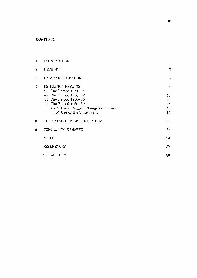
CONTENTS

1 INTRODUCTION

2 METHOD

3 DATA AND ESTIMATION

4 ESTIMATION RESULTS 4.1 The Period 1951-61 4.2 The Period 1960-77 4.3 The Period 1958-80 4.4 The Period 1960-80

4.4.1 Use of Lagged Changes in Income 4.4.2 Use of the Time Trend

5 INTERPRETATION OF THE REST-TLTS

6 CONCLUDING REMARKS

NOTES

REFERENCES

THE AUTHORS

DYNAMIC ESZllldATION OF THE CONSUMER DEMAND S Y m M IN POSlWAR JAPAN

Kozo Sasaki and Yoshihiro Fukagawa

1 INTRODUCTION

This report explores the dynamic demand relations operative in Japan in the period 1951-80. Consumption levels and patterns have shifted so drasti- cally over the last thirty years that i t is of great interest to elucidate the dynamic nature and characteristics of the varied structures of consumer demand during the entire period. Special attention is given to the analysis of structural change in more recent years.

This study also aims a t evaluating empirical evidence of the dynamic structure of consumer demand in the postwar period. It is an extension of a previous study (Sasaki 1982) in which both static and dynamic models of the linear expenditure system were fitted to time series of family budget data for the period 1951-77.

The same method is adopted here: a simplified version of the linear expenditure system extended by A. A. Powell for the sake of computational convenience. The expenditure and price data used in the earlier study were updated, adding three more years to the time series. Five alternative specifications of the taste variable were utilized here in order to take due account of recent structural changes in consumer demand. The first two are based on current annual increase in income and on current annual rate of increase in income, which can be seen in some of the conventional demand analyses in econometric models. The next two incorporate lagged annual increase in income and lagged annual rate of increase in income, and the last specification is based on the t ime trend.

The commodity definition used is described in more detail below. With respect to the previous study, the original 24 subgroups have been adjusted somewhat, yielding a 21-commodity breakdown for all the cases under con- sideration. Moreover, Inany individual segments of the total observation period were chosen for estimating the dynamic model. All these changes were made to satisfy more closely the theoretical constraints imposed on the model and to obtain, as far as possible, a good fit between the model and the empirical data.

We also felt i t was of some interest to examine the stability of such important parameters as money flexibility, subsistence consumption levels,

etc., when a particular specification of the taste variable is introduced into the expenditure functions.

The estimation results for many different cases could, in principle, be compared in various respects. However, this study concentrates on just four subperiods with fairly good results for detailed discussion. Note that most of the statistical tests used are implemented under linear least-squares postu- lates.

2 METHOD

A complete set of linear expenditure functions is used, explaining per capita expenditure on each commodity in terms of all prices, per capita income, and the taste variable. Under the given assumptions, the estimating equation of Powell's system takes the form:

where

and

ut = m t - C p . ,tzj - ( i , j = 1,2 , . . . , N ) , ( t = 1,2 , . . . , T) j

The notation used here is as follows: pi and xi are the price and quantity consumed per capita, m the per capita income, s the taste variable, and ci the error term. pi is the sample mean of pi and ?ti is the ratio of the sample mean expenditure to the mean price pi. zi and u indicate substitution and income variables, respectively. The subscripts i and j are commodity indices, and t denotes time. The A, bi, and ci are unknown parameters. More specifically. A has the following properties:

and

A = m - C pipi (Pi = subsistence consumption level) i

(3)

where 13 is money flexibility, which is equivalent to the income elasticity of the marginal utility of income. p is called income flexibility and is the reciprocal of w'. Then A is interpreted as the supernumerary income. bi represents the marginal budget stlare and ci denotes the coefficient of the taste variable s t .

The taste variable st can be specified in an appropriate way as the occa- sion requires. Leser (1960) noted tha t i t is easy to estimate a set of regres- sion equations with the same independent variables, but disregarding the zit variable, under least-squares assumptions.' In accordance with Leser's argu- ment, Powell's version of the linear expenditure system (Powell 1966) also contains a dynamic factor common to all equations, which allows for shifts in expenditure and demand functions.

In the present analysis, taste changes are represented by a single vari- able st in order to facilitate estimation by a systems least-squares method. The dynamic model is fitted for various phases of the period studied, with alternative specifications of a proxy for the taste variable. In the first place, two alternative expressions are taken into account: current annual increase in income and current annual rate of increase in income:

st = mt - mt-l and st = (mt - mt-l) /mt- l (4)

These expressions are applied uniformly to all cases involving different sample periods. For more recent periods, which the above specifications do not fit well, three different alternative expressions are incorporated separately into the estimating equation (1). These are written as:

't = mt-1 - and st = (mt-l - mt -2), mt-2

and

Equation (5) is the same as eqn. (4), except that the former has a one- year lag. I t simply suggests that, in recent years, the consumer has responded more slowly to either annual increments in or the annual growth rate of real income.

The dynamic model is assumed to satisfy the homogeneity condition only a t the mid-point of the sample period. In cases where the model uses deflated expenditure and price data, however, all current (or nominal) expenditure functions are homogeneous of degree one in current prices, current income, and the General Consumer Price Index (hereafter referred to as the CPI). I t is apparent that the corresponding demand Iunctions are homogeneous of degree zero in current prices and income.

3 DATA AND ESI'WI'ION

The data sources on per capita expenditures and prices are the Annual Reports published by the Office of the Prime Minister, Japan (1950-1980). Data for all households in cities with a population of 50,000 or more are util- ized in this study, since long t ime series are available on expenditures and prices in the postwiir period. Price indexes in the Laspeyres form are avail- able for all subgroups and these are taken as individual prices for each sub- group, with all of the 1970 indexes being set a t unity. Hence, the associated quantities represent expenditures in constant 1970 yen.

The commodity grouping on which the study is based is shown in Table 1. In practice, a 21- rather than 24-commodity breakdown is generally employed here by combining several of the original subgroups into broader groups. This results in two commodity lists, which differ slightly from each other as can be seen in some of the Iollowing tables. All the time series used cover the period 1951-80.

It should be noted that both the expenditure and the price data are deflated by the CP1 so as to ensure that consumer demand in the model does not respond to changes in nominal prices, but to changes in relative prices.

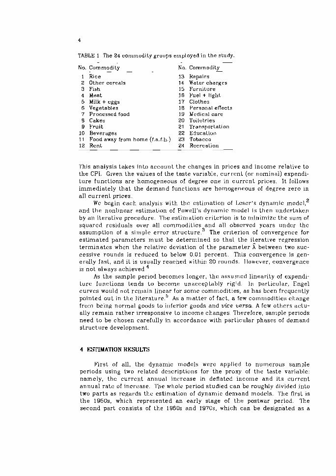
TABLE 1 The 24 commodity groups employed in the study.

No. Commodity No. Commodity

1 Rice 13 2 Other cereals 14 3 Fish 15 4 Meat 16 5 Milk + eggs 17 6 Vegetables 18 7 Processed food 19 B Cakes 20 9 Fruit 21

10 Beverages 22 11 Food away from home (f.a.f.h.) 23 12 Rent 24

Repairs Water charges Furniture Fuel + Light Clothes Personal effects Medical care Toiletries Transportation Education Tobacco Recreation --

This analysis takes into account the changes in prices and income relative to the CPI. Given the values of the taste variable, cu r ren t (or nominal) expendi- t u re functions are homogeneous of degree one in cur rent prices. I t follows immediately tha t the demand functions are homogeneous of degree zero in a11 cu r ren t prices.

We begin each analysis with the est imation of Leser's dynamic model, 2

and the nonlinear estimation of Powell's dynamic model is then undertaken by an i terat ive procedure. The estimation criterion is to minimize the sum of squared residuals over a11 commodities and all observed years under the assumption of a simple error ~ t r u c t u r e . ~ The criterion of convergence for est imated parameters must be determined so tha t the i terat ive regression terminates when the relative deviation of the parameter between two suc- cessive rounds is reduced to below 0.01 percent. This convergence: is gen- erally fast, and i t is usuaIly reached within 20 rounds. However, convergence is not always a ~ h i e v e d . ~

As the sample period becomes longer, the assumed linearity of expendi- t u re functions tends t o become unacceptably rigid. In part icular, Engel curves would not remain linear for some commodit.ies, as has been frequently pointed out in the ~ i t e r a t u r e . ~ As a ma t te r of fact, a few commodities change from being normal goods to inferior goods and vice versa. A few others actu- ally remain ra ther irresponsive to income changes. Therefore, sample periods need to be chosen carefully in accordance with part icular phases of demand s t ruc ture development.

4 ESTIMATION RESULTS

First of all, t he dynamic models were applied to numerous sample periods using two related descriptions for the proxy of the taste variable: namely, the c-urrent annual increase in deflateti income and i ts cur rent annual ra te of increase. The whole period studied can be roughly divided into two pa r t s as regards the estimation of dynamic demand modc:ls. The first is t h e 1950s, which represented an early stage of the postwar period. The second part consists of the 1960s and 1970s, which can be designated as a

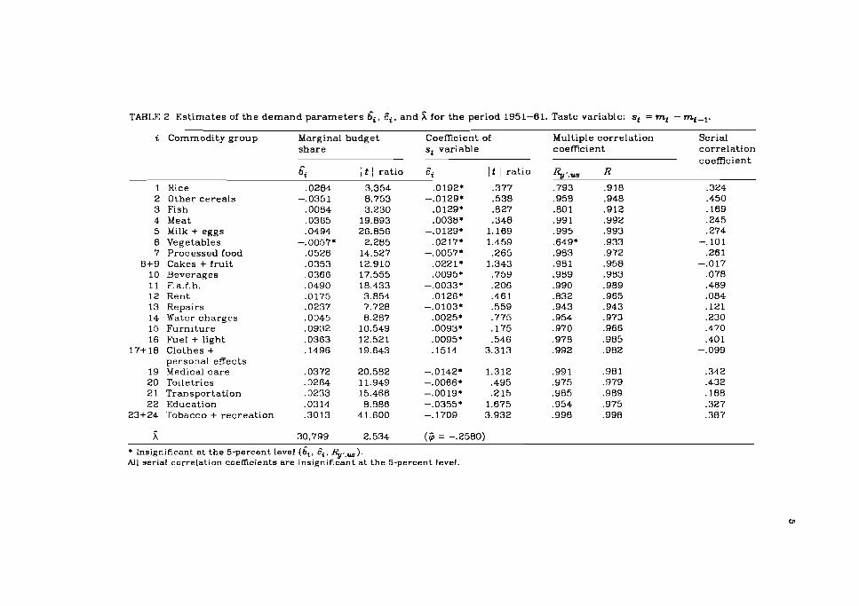
TABLE 2 Estimates of the demand parameters gin Ei, and for the period 1951-61. Taste variable: st = 9 - mt-*.

i Commodity group Marginal budget Coefficient of Multiple correlation Serial share st variable coefficient correlation

coefficient Ki It 1 ratio 4 It 1 ratio , R

1 Rice ,0284 3.354 .0192* .377 .793 .918 .324 2 Other cereals -.0351 8.753 -.0129* .538 ,958 .948 .450 3 Fish ,0084 3.230 .0129* .827 .801 .912 .I69 4 Meat ,0365 19.893 .0038* .348 .99 1 .992 ,245 5 Milk + eggs .0494 26.856 -.0129* 1.169 ,995 .993 ,274 6 Vegetables -. 0057* 2.285 .0217* 1.459 .649* ,933 -. 101 7 Processed food .0526 14.527 -.0057* .265 .983 ,972 .261

8+9 Cakes + fruit .0353 12.910 .0221* 3.343 ,981 .958 -.017 10 Beverages ,0366 17.555 .0095* ,759 .989 .983 ,078 11 F.a.f.h. ,0490 18.433 -.0033* .206 ,990 .989 .469 12 Rent .0175 3.854 .0126* ,461 .832 ,965 ,084 13 Repairs .0237 7.728 -.0103* ,559 ,943 ,943 ,121 14 Water charges ,0045 8.287 .0025* .775 .954 ,973 ,230 15 Furniture ,0932 10.549 .0093* .I75 ,970 .966 ,470 16 Fuel + light ,0363 12.521 .0095* .546 .978 ,985 ,401

17+18 Clothes + .I496 19.643 .I514 3.313 .992 ,982 -.099 personal effects

19 Medical care .0372 20.582 -.0142* 1.312 .991 .981 .342 20 Toiletries .0264 11.949 -.0086* .495 .975 .979 .432 21 Transportation ,0233 15.466 -.0019* ,215 .985 .989 ,188 22 Education .03 14 8.886 -.0355* 1.675 ,954 ,975 .327

23+24 Tobacco + recreation .3013 41.600 -. 1709 3.932 .998 ,998 .387

Insignificant at the 5-percent level (&, E,, %..,). All serial correlat~on coefficients are insignificant at the 5-percent level

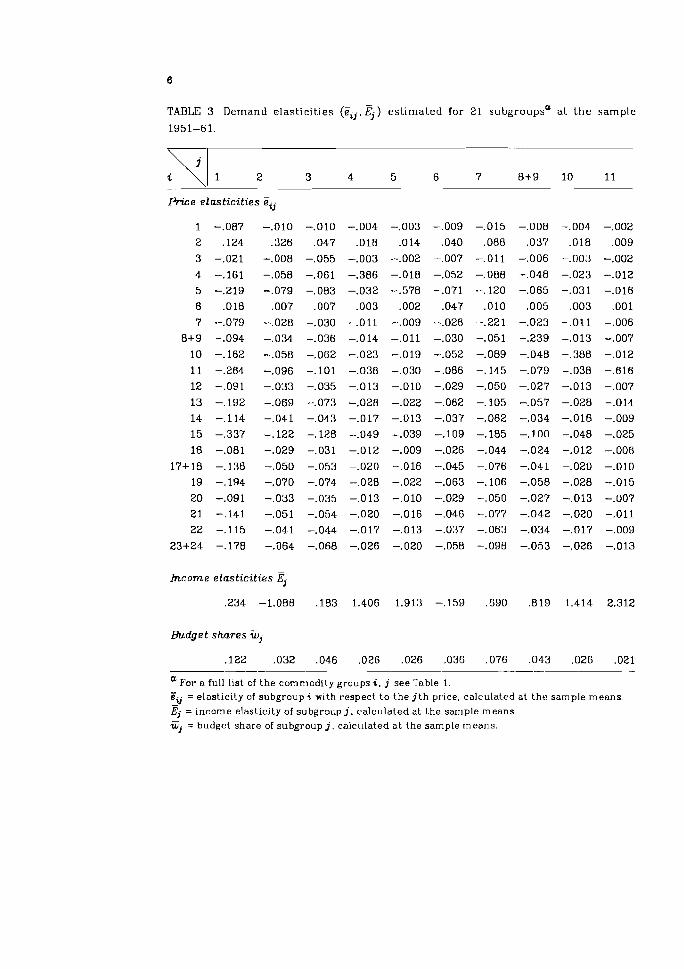
TABLE 3 D e m a n d e las t i c i t i es (eii.6) e s t i m a t e d for 2 1 subgroupsa a t t h e s a m p l e

1951-61.

Price e las t ic i t ies Fij

h c o m e e las t ic i t ies

Budget shares Gj

a For a full list of the commodity groups i, j see Table 1.

Zij = elast ic i ty of srlbgroup i with respect t o t h e j t h price, calculated a t t h e sample means

Ej = income elasticity of subgroup j, calculated at the sample means. G . = budget share of subgroup j, calculated a t the sample means. J

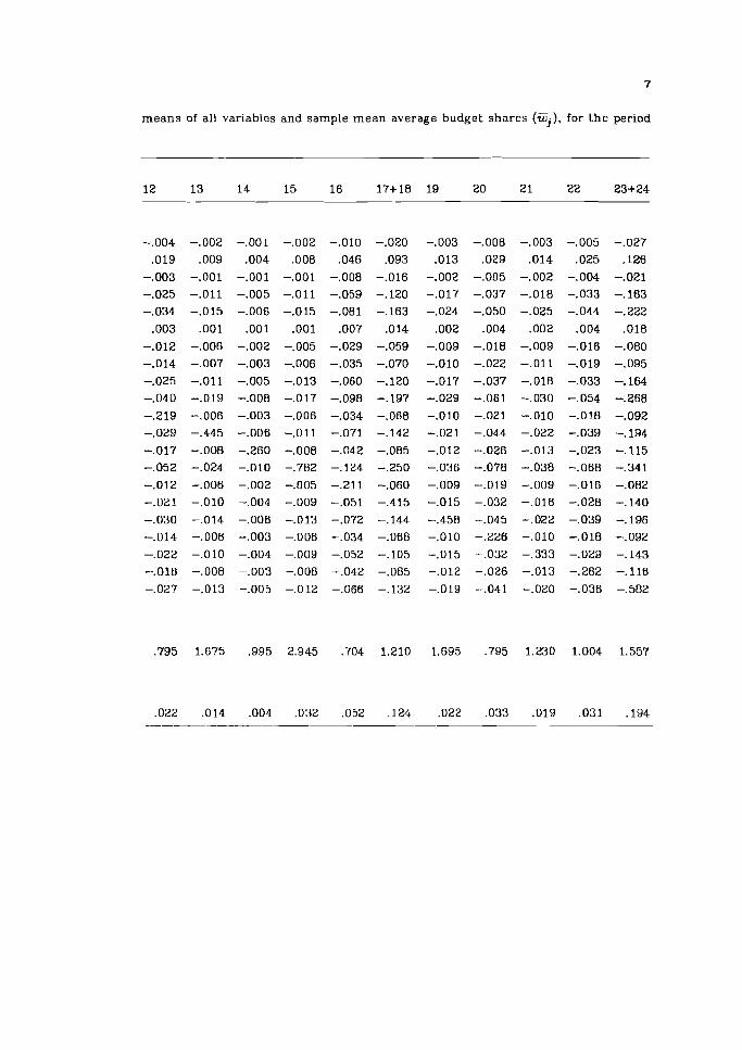
means of all variables and sample mean average budget shares (W,), for the period

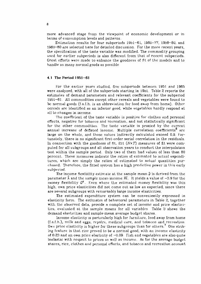
more advanced stage from the viewpoint of economic development or in terms of consumption levels and patterns.

Estimation results for four subperiods 1951-61, 1960-77, 1958-80, and 1960-80 are selected here for detailed discussion. For the more recent years, the specification of the taste variable was modified. The commodity grouping used for earlier subperiods is also different from that of recent subperiods. Great efforts were made to enhance the goodness of fit of the models and to handle as many normal goods as possible.

4.1 The Period 1951-61

For the earlier years studied, five subperiods between 1951 and 1965 were analyzed, with all of the subperiods starting in 1951.. Table 2 reports the estimates of demand parameters and relevant coefficients for the subperiod 1951-61. All commodities except other cereals and vegetables were found to be normal goods (f.a.f.h. is an abbreviation for food away from home). Other cereals are identified as an inferior good, while vegetables hardly respond a t all to changes in income.

The coefficient of the taste variable is positive for clothes and personal effects, negative for tobacco and recreation, and not statistically significant for the other commodities. The taste variable is proxied by the current annual increase of deflated income. Multiple correlation coefficients6 are large on the whole, and those values indirectly calculated exceed 0.9. For- tunately, there is no significant first-order serial correlation in the residuals. In connection with the goodness of fit, 231 ( N x T ) measures of fit were com- puted for all subgroups and all observation years t o conduct the interpolation test within the sample period. Only two of them had values of less than 80 percent. These measures indicate the ratios of estimated to actual expendi- tures, which are simply the ratios of estimated to actual quantities pur- chased. Therefore, the fitted system has a high predictive power in this early subperiod.

The inc_ome flexibility estimate a t the sample mean is derived from the parameter X and the sample mean income E. I t yields a value of -3.9 for the money flexibility G e . Even where the estimated money flexibility was this high, own price elasticities did not come out as low as expected, since there are several subgroups with remarkably large income elasticities.

The estimated expenditure system can be conveniently expressed in elasticity form. The estimates of behavioral parameters in Table 2, together with the observed data, provide a complete set of income and price elastici- ties, evaluated a t the sample means for all variables. Table 3 shows the demand elasticities and sample-mean average budget shares.

Income elasticity is particularly high for [urniture, Iood away from home (f.a.i.h.), milk and eggs, repairs, medical care, and tobacco and recreation. Owrl price elasticity is higher for these subgroups than for other^.^ One strik- ing feature is that rice proved to be a normal good, with an income elasticity of 0.23 and an own price elasticity oi -0.09. Fish and vegetables are also quite inelastic with respect to prices as well as income. As for the average budget shares, rice, clothes and personal effects, and tobacco and recreation account

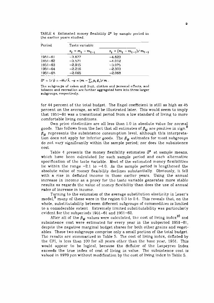
TABLE 4 Estimated money flexibility 2jB by sample period in the earl ier years studied.

Period Taste variable

The subgroups of cakes and fruit, clothes and personal effects, and tobacco and recreation ere further aggregated here into three larger subgroups, respectively.

for 44 percent of the total budget. The Engel. coefficient is still as high as 45 percent on the average, as will be il lustrated later. This would seem to imply that 1951-61 was a transitional period from a low standard of living to more comfortable living conditions.

Own price elasticities are all less than 1.0 in absolute value for normal goods. This follows from the fact that all est imates of pit are positive in sign.' pit represents the subsistence consumption level, although th is interpreta- tion does not apply for inferior goods. The pit estimates for most subgroups do not vary significantly within the sample period; nor does the subsistence cost.

Table 4 presents the money flexibility estimates w" at sample means, which have been calculated for each sample period and each alternative specification of the taste variable. Most of the estimated money flexibilities lie within the range -2.1 to -4.0. As the sample period is lengthened the absolute value of money flexibility declines substantially. Obviously, i t fell with a rise in deflated income in those earlier years. Using the annual increase in income as a proxy for the taste variable generates more stable results as regards the value of money flexibility than does the use of annual r a t e s of increase in income.

Turning to the estimates of the average substitution elasticity in Leser's model,' many of these were in the region 0.3 to 0.4. This reveals that , on the whole, substitutability between different subgroups of commodities is limited to a considerable extent. Extremely limited substitutability was particularly evident lor the subperiods 1951-61 and 1951 -62.

After all of the pit values were calculated, the cost of living index1' and subsistence cost were estimated for every year in the subperiod 1961-61., despite the negative marginal budget shares for both other grains and veget- ables. These two subgroups comprise only a small portion of the total budget. The results are summarized in Table 5. Th.e cost of living index, deflated by the CPI, is less than 100 for all years other than the base year, 1951. This would appear to be logical, because the deflator of the 1,aspeyres Index exceeds the t rue index of cost of living in value. The subsistence cost is valued in 1970 yen without modification by the cost of living index in Table 5.

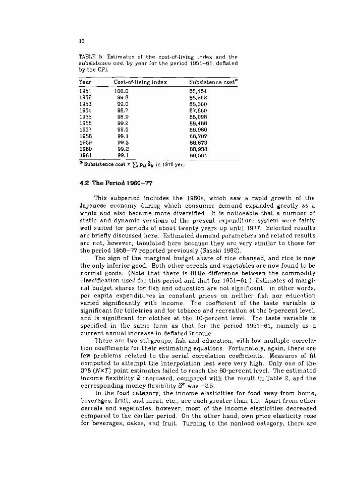
TABLE 5 Estimates of the cost-of-living index and the subsistence cost by year for the period 1951-61, deflated by the CPI.

Year Cost-of-living index

1951 100.0 1952 99.6 1953 99.0 1954 98.7 1955 98.9 1958 99.2 1957 99.5 1958 99.1 1959 99.3 1960 99.2 1981 99.1

a Subsistence cost = z , p u Bit in 1970 yen.

Subsistence costa

4.2 The Period 1960-77

This subperiod includes the 1960s, which saw a rapid growth of the Japanese economy during which consumer demand expanded greatly as a whole and also became more diversified. It is noticeable that a number of static and dynamic versions of the present expenditure system were fairly well suited for periods of about twenty years up until 1977. Selected results are briefly discussed here. Estimated demand parameters and related results are not, however, tabulated here because they are very similar to those for the period 1958-77 reported previously (Sasaki 1982).

The sign of the marginal budget share of rice changed, and rice is now the only inferior good. Both other cereals and vegetables are now found to be normal goods. (Note that there is litt le difference between the commodity classification used for this period and that for 1951-61.) Estimates of margi- nal budget shares for Ash and education are not significant: in other words, per capita expenditures in constant prices on neither fish nor education varied significantly with income. The coefficient of the taste variable is significant for toiletries and for tobacco and recseation a t the 5-percent level, and is significant for clothes a t the 10-percent level. The taste variable is specified in t-he same form as that for the period 1951-61, namely as a current annual increase in deflated income.

There are two subgroups, fish and education, with low multiple correla- tion coefficients for their estimating equations. Fortunately, again, there are few problems related to the serial correlation coefficients. Measures of fit computed to at tempt the interpolation test were very high. Only one of the 378 ( N x T ) point estimates failed to reach the 80-percent level. The estimated income flexibility $ increased, compared with the result in Table 2, and the corresponding money flexibility Ze was -2.5.

In the food category, the iricome elasticities for food away from home, beverages, fruit, and meat, etc., are each greater than 1.0. Apart from other cereals and vegetables, however, most of Che income elasticities decreased compared to the earlier period. On the other hand, own price elasticity rose for beverages, cakes, and fruit. Turning to the nonfood category, there are

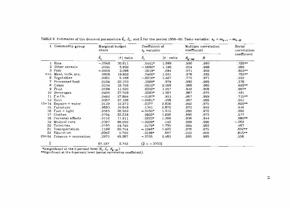
TABLE 6 Estimates of the demand parameters gi, Ei. and 5; for the period 1958-80. Taste variable: st = rnt-l - r n t - ~ .

i Commodity group

1 Rice 2 Other cereals 3 Fish

4+5 Meat, milk, etc. 6 Vegetables 7 Processed food 8 Cakes 9 Fruit

10 Beverages 11 F.a.f.h. 12 Rent

13+ 14 Repairs + water 15 Furniture 16 Fuel + light 17 Clothes 18 Personal effects 19 Medical care 20 Toiletries 21 Transportation 22 Education

23+24 Tobacco + recreation

Marginal budget share

b ,̂ It ( ratio

-.0546 30.811 .0035 5.838

-.0048 3.096 ,0626 19.950 ,0061 5.168 .0194 22.073 .0134 16.706 .0198 11.520 .0406 27.709 ,0462 27.864 ,0357 27.198 ,0139 12.373 .0683 18.648 ,0525 28.509 ,0794 22.238 ,0152 11.911 .0397 88.200 ,0195 24.745 ,1199 20.754 ,0062 2.700 .3973 45.287

Coefficient of st variable

Multiple correlation coefficient

Ei It 1 ratio

Serial correlation coefficient

*Insignificant a t the 5-percent level (g i , 4, %.,,). **Significact a t the 5-percent level (serial correlation coefficient).

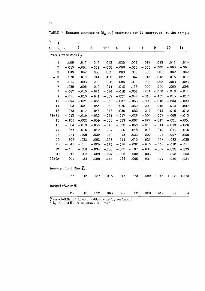
TAEILE 7 Demand elasticities ( F i j , E,) estimated for 21 subgroupsa at the sample

Price e las t ic i t ies Fij

h c o m e e las t ic i t ies Ej

Budget shares G,

a For %full list of the commodity groups i, j see Table 1. G , E,. and Gj are as defined in Table 3.

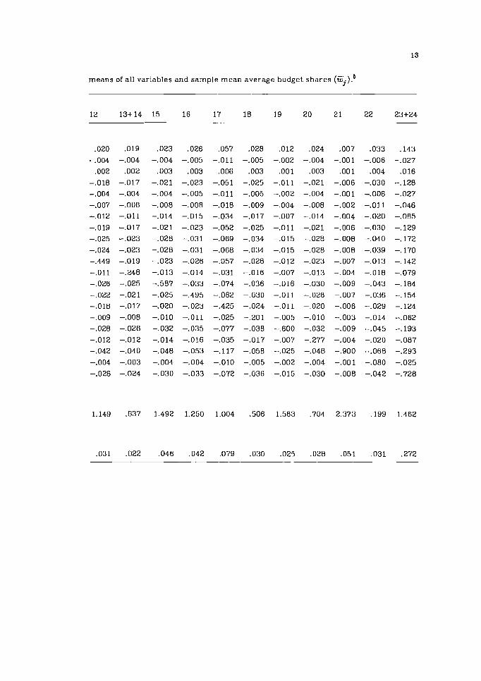
means of all variables and sample mean average budget shares (G,).*

quite a few subgroups whose income elasticities exceed 1.0. Demands for transportation, medical care, furniture, and recreation are all highly respon- sive to income changes. The absolute values of own price elasticity increased conspicuously for transportation, medical care, recreation, and rent, and for fuel and light. Own price elasticities were all less than 1.0 in absolute value, which stems from the fact that all of the pit estimates were positive.

The average budget shares for rice and other cereals are much smaller than before. Those for food away from home, meat, milk and eggs, and bever- ages apparently went up. Of the nonfood subgroups, recreation and transpor- tation sharply expanded their shares of the total budget. Money flexibilities are found to be rather stable in the three subperiods 1958-77, 1959-77, and 1960-77, falling in the range -2.1 to -2.7. The estimates for 1958-79, how- ever, fell some distance outside this range. Moreover, the specification of the taste variable used here does not seem to be suitable for more recent years. This issue will be discussed later. Leser's elasticities of substitution were estimated a t between 0.6 and 0.7, except for the period 1951-77, for which the values were slightly greater than 1.0

4.3 The Period 1958-80

The specifications of the taste variable described above did not prove suitable for estimating the dynamic model for more recent years. Moreover, the static model did not fit the latest data sets. Accordingly, another pair of taste variables were implemented separately for the estimation of dynamic expenditure systems: namely, a lagged annual change in deflated income and a lagged annual rate of change in deflated income. For this purpose, a one- year lag was applied to the previous taste variables. The resulting, new taste variables are predetermined variables in the expenditure system, and they produced good results for some cases covering more recent years.

Some examples of tht: results are shown in Table 6 in terms of estimated demand parameters and related coefficients. The marginal budget share now takes a negative value for fish as well as for rice. The growth of expendi-ture in constant prices on fish was so low in the past that the income responsive- ness of fish consumption turned out to be insignificant for the period 1960-77. Over a longer period of time, such as the present subperiod, 1958-80, the income elasticity of fish declines to a negative value. It is fre- quently said that the reduction in fish consumption as a whole has been due to the sharp increase in its price associated with changes in fish-supply con- ditions in recent years, changes in quality, and so on. All subgroups other than rice and fish are normal goods.

The coefficient of the taste variable is significantly different from zero a t the 5-percent significance 1t:vel for three subgroups: repairs and water, furni- ture, and tobacco and recreation. A t the 10-percent level, by comparison, i t is significant for five more subgroups as far as the t-ratio test is concerned: these are rice, cakes, fuel and light, clothes, and toiletries.

Multiple correlation coefficients are all significant, but nearly half of all the subgroups have positive serial correlation in the residuals. Measures of fit in the interpolation test were mostly 80 percent or more. Of the 483 ( N x T)

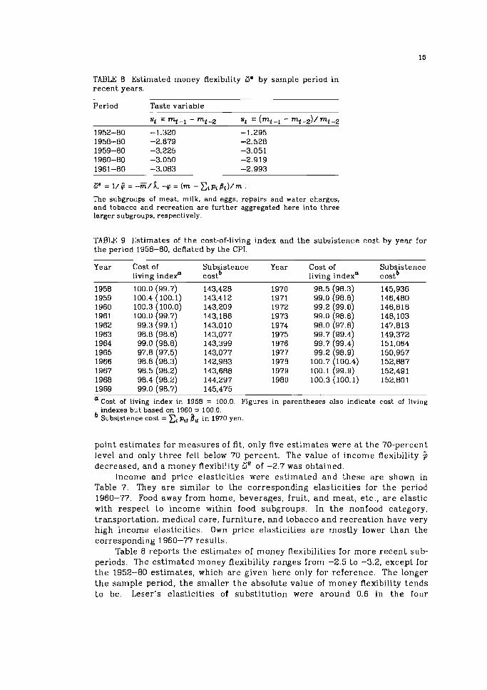
TABLE 8 Estimated money flexibility 2js by sample period in recent years.

Period Taste variable

st = nt - mt -Z st = (mi -1 - mt -2)/ mi -2

1952-80 -1.320 -1.295 1958-80 -2.679 -2.528 1959-80 -3.225 -3.051 1960-80 -3.050 -2.919 1961-80 -3.083 -2.993

The subgroups of meat, milk, and eggs, repairs and water charges, and tobacco and recreation are further aggregated here into three larger subgroups, respectively.

TABLE 9 Estimates of the cost-of-living index and the subsistence cost by year for the period 1958-80, deflated by the CPI.

Year Cost of Subsistence Year Cost of Subsistence living indexa costb living indexa costb

a Cost of living index in 1958 = 100.0. Figures in parentheses also indicate cost of living indexes but based on 1960-= 100.0. Subsistence cost = z i p , * flu in 1970 yen.

point estimates for measures of fit, only five estimates were a t the 70-percent level and only three fell below 70 percent. The value of income flexibility 5 decreased, and a money flexibility Ge of -2.7 was obtained.

Income and price elasticities were es?iinated and these are shown in Table 7. They are similar to the corresponding elasticities for the period 1960-77. Food away from home, beverages, fruit, and meat, etc., are elastic with respect to income within food subgroups. In the nonfood category. trarisportation, medical care, furniture, and tobacco and recreation have very high income elasticities. Own price elasticities are rnostly lower than the corresponding 1960-77 results.

Table 8 reports the estimates of money flexibilities for more recent sub- periods. The estimated money flexibility ranges from -2.5 to -3.2, except for the 1952-80 estimates, which are given here only for reference. The longer the sample period, the smaller the absolute value of money flexibility tends to be. Leser's elasticities of substitution were around 0.6 in the four

subperiods, while those for the 1952-80 period were close to 1.0. All pit estimates were found to have positive values and to change, to a

greater or lesser extent, from year to year. The cost of living index and sub- sistence cost by year, computed from estimated demand parameters and observed data, are presented in Table 9. Incidentally, these results for the individual years between 1960 and 1977 were comparable with those obtained for the whole period 1960-77 and examined in Section 4.2.

4.4 The Period 1960-80

For this period, two model formulations were employed. The first, and less successful approach used the lagged annual change in deflated income for the taste variable in the same way a s described in earlier sections. The second approach utilized a t ime trend as a proxy for the taste variable. The results for each method will now be briefly described.

4.4.1 Use of Lagged Changes in Income The lagged annual change in deflated income was again found to play a

role in changes in tastes, although using this kind of taste variable shed little light on the dynamic factors a t work. Rice and fish have negative marginal budget shares while all other subgroups have positive ones. Repairs and water, and furniture, have positive coefficients for the taste variable while tobacco and recreation show a negative coefficient a t the 5-percent significance level. A t t he 10-percent level, the coefficient of the taste variable is positive for rice and cakes, but negative for fuel and light. These data are not tabulated here because they are very similar to the results in Table 6 for the period 1958-80.

4.4 .2 Use of the Zime Trend Since none of the specifications of the taste variable described earlier

worked particularly well in. identifying dynamic factors affecti.ng the ex:pendi- ture system, a time trend. mechanism was incorporated in the model. This version of the model has been fitted to four data sets in recent years, and i t has been found that the t ime trend serves rather well as a proxy for the taste variable over relatively long t ime series.

The period 1960-80 is singled out here for more detailed discussio.n, and the relevant data are given in the following two tables. Table 10 indicates that the coefficient of the t ime trend is statistically significant for two-thirds of all subgroups of commodities. The t rend variable exerts a significantly positive effect on four subgroups, including food away from home and trans- portation, and i t has a negative coefficient for ten other subgroups. For the remaining subgroups i t does not seem to have any significant influence.

Rice is certainly an inferior good. All other commodities are normal goods except other cereals, food away from home, transportation, and educa- tion, which are irresponsive to income change. The multiple correlation coefficients, whether or not they are adjusted for degrees of freedom, tend to be greater and the serial correlation in the residuals is much less serious in Table 10 than in Table 6. The interpolation test resulted in high measures of

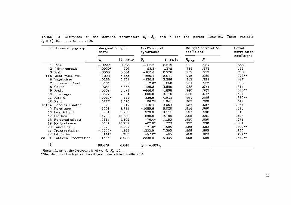
TABLE 10 Estimates of the demand parameters &. I?=. and for the period 1960-80. Taste variable: st = t(-10.. . . , -1,O.l.. . . -10).

i Commodity group

1 Rice 2 Other cereals 3 Fish

4+5 Meat. milk. etc. 6 Vegetables 7 Processed food 8 Cakes 9 Fruit

10 Beverages 11 F.a.f.h. 12 Rent

13+14 Repairs + water 15 Furniture 16 Fuel + light 17 Clothes 18 Personal effects 19 Medical care 20 Toiletries 21 Transportation 22 Education

23+24 Tobacco + recreation

Marginal budget share

& It 1 ratio

-. 0292 2.985 -.0030* .707

.0360 5.351 ,1203 5.854 ,0288 6.761 ,0161 3.032 ,0285 6.868 ,0662 6.624 ,0677 7.524 ,0024' 2 8 9 ,0277 3.040 .0372 6.917 ,1552 7.844 ,0201 2.958 ,1762 16.660 ,0224 3.169 ,0427 10.939 ,0273 5.297

-.0055* ,295 .0114* ,735 ,1515 3.920

Coemcient of st variable

Multiple correlation coefficient

It 1 ratio

2.519 1.375 2.930 3.011 3.366 ,350

3.559 4.898 3.716 4.512 1.041 2.953 6.020 6.111 9.186 1.183 .779

1.505 7.303 .405

6.335

Serial correlation coefficient

'Insignificant at the 5-percent level (&, 4, %.,,). **Significant at the 5-percent level (serial correlation coefficient)

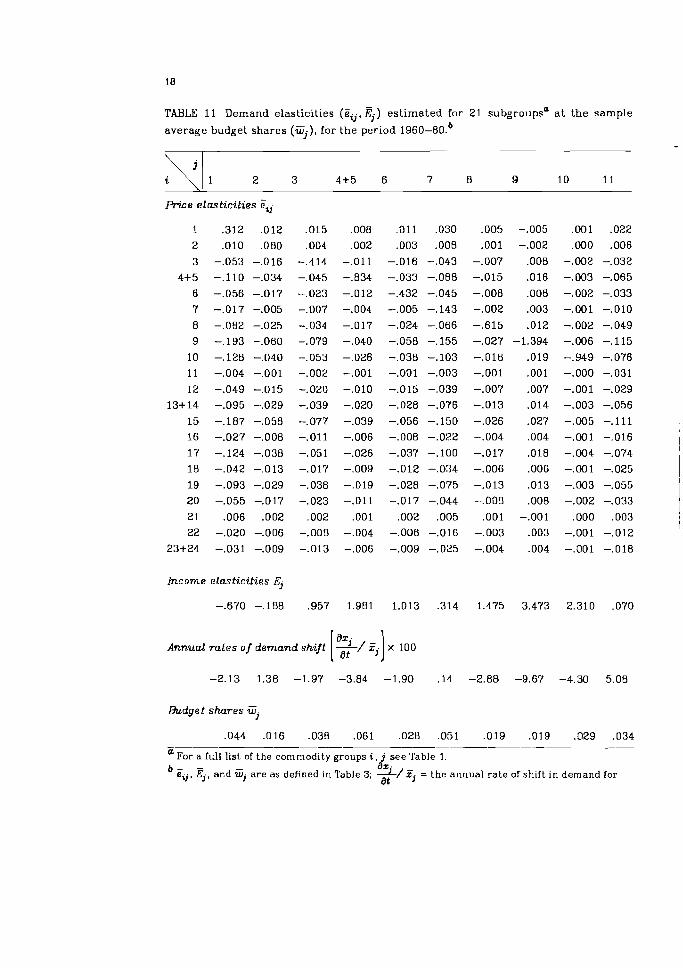
TABLE 11 Demand elasticities (q j . 6 ) est imated for 21 subgroupsa a t the sample

average budget shares (q), for the period 1960-80.~ -

2 3 4+5 6 7 8 9 10 11

Price elasticities eij

Encome elasticities E,

Annual rates of demand shift -/ F,. x 100 [2 ]

Budget shares

a For a full list of the cornrnodity groups i , j see Table 1. b - az. e ~ . E,, and Gj are as defined in Table 3; -/ 3 = the annual rate of shift in demand for

at

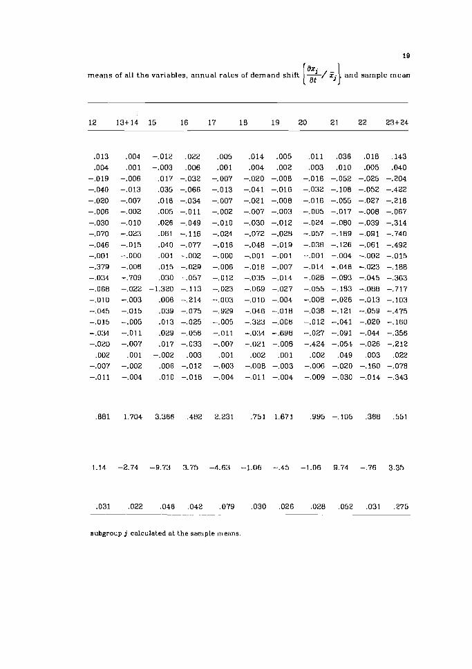
means of all the variables, annual rates of demand shift [? -/ z. -,] , and sample mean

subgroup j calculated a t the sample means

fit. Only two of the 441(NxT) measures of fit were less than 80 percent. Table 11 presents the demand elasticities, annual rates of demand shift,

and average budget shares, calculated at sample means. Fruits, beverages, furniture, and clothes have large income elasticities that exceed 2.0. Demand for these subgroups, however, shifts substantially downward year after year, other things being equal. On the other hand, demands for food away from home, fuel and light, transportation, and recreation increase annually, while their income elasticities are quite low.

For the subperiods 1957-80, 1958-80, 1959-80, and 1960-80, estimates of money flexibility a t the mid-point were -2.5, -2.7, -2.8, and -2.4, respec- tively. The corresponding estimates for Leser's elasticity of substitution were 0.89, 0.76, 0.68, and 0.70. The estimated money flexibilities were rather stable.

As some pit estimates have negative values for the period 1960-80 and as there are three subgroups with a negative marginal budget share, we do not propose to discuss here the cost of living index or the subsistence cost for this period.

5 INTERPRETATION OF THE RESULTS

Based on the estimation results for the above four subperiods, demand elasticities and average budget shares can be derived a t sample mean levels by subperiod for the two broad categories of food and nonfood. The demand elasticities are obtained from the estimates of income and price elasticities for 21 subgroups of commodities and their sample mean average budget shares, by using Engel aggregation, Cournot aggregation, and the homo- geneity condition.'' Table 12 shows the derived income and price elasticities and average budget shares for food and nonfood in the four sample periods. For the period 1960-80 annual ra tes of shift in demand a t sample means are also presented. The rate of shift for food is -1.9 percent per annum, while both income and price elasticities are appreciably higher than expected.

The derived demand elasticities varied across the sample periods. On examination of the results for the flrst three periods, i t is clear that income and price elasticities for food have been diminishing in absolute terms over t ime. This is reflected in the fact that. the average budget share of food (or Engel coefficient) declines as per capita income grows. The demand for food is more susceptible to income and food price than to nonfood price. Cross price elasticities take negative values, satisfying the theoretical features of the linear expenditure system.12 This indicates that the income effect of a change in price exceeds the substitution effect, and that the estimates a t sample means are positive and can be interpreted as subsistence consump- tion levels.

According t o the analysis of the 21-commodity breakdown, all est imates of pit were positive in the first three subperiods, where own price elasticities were all less than 1.0 in absolute value. Meanwhile, income elasticities were particularly high for such nonfood subgroups as transportation, medical care, furniture, and recreation during the whole period studied. Rent, as well a s fuel and light, exhibited an upward tendency in income elasticity. It is

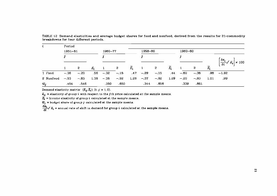
TABLE 12 Demand elasticit ies and average budget shares for food and nonfood, derived from the results for 21-commodity breakdowns for four different periods.

Period

- - - I "" I 1 2 Ei 1 2 Ei 1 2 4 1 2 G

1 Food -.36 -.20 .56 -.32 -.I5 .47 -.29 -.I5 .44 -.60 -.38 .98 -1.92

Demand elasticity matrix: (Fv 4); (i. j = 1,2). o;j = elasticity of group i with respect to the j t h price calculated a t the sample means.

4 = income elasticity of group i calculated at the sample means. Gj = budget share of group j calculated at the sample means.

4 = annual rate of shift in demand for group i calculated at the sample means.

beyond question that larger and higher-quality housing continues to be in great demand. At the same t ime, beverages, food away from home, fruit , and meat all exhibit high income elasticities.

I t is clear that these commodity groups with high income elasticity have been rising in their relative position in total expenditure. Rice arid other cereals, which have a negative or low income elasticity, have dropped remarkably in their share of the consumer's budget. As a result, income is considered the most important factor in allocating the total budget between different commodities, always assuming that annual increment in income or the annual growth rate thereof is used for the taste variable.

A brief illustration of the changes in prices and their influence on con- sumption patterns may be useful a t this point. Over the period 1958-80, for instance, the current price increased 10 t imes for fish, 9 t imes for veget- ables, 6 t imes for other cereals, 5.7 t imes for food away from home, and 5 t imes for rice, whereas there was a 4.4-times rise in the CPI. Other subgroups of food commodities advanced relatively slowly in current price. Of the non- food subgroups, education and repairs each went up 8 t imes, and rent advanced 6 t imes in price during the period 1958-80. Increases in other prices were relatively small.

No sharp drop was observed in the expenditures in constant prices on flsh, vegetables, food away from home, rent , or education, etc., whose prices jumped markedly during the period in question. This suggests that consump- tion was affected more by income and probably by various dynamic factors than by relative prices. Except for food away from home and rent , the latter subgroups seem to have ceased to grow in terms of per capita consumption.

As is widely recognized, money flexibility estimates are sensitive to differences in the sample period, commodity classification, model specification, whether the model version is stat ic or dynamic, the type of proxy variable used for changing tastes, and so on. On the basis of results for the same commodity classification and model specification, there is some indication tha t the longer the sample period, the greater the money flexibil- ity in algebraic terms. Since own price elasticities are closely related to the magnitude of money flexibility, they are likely to become larger in absolute value over a longer period of time. Thus, money flexibility is to a large extent associated with substitutability between commodities. For these reasons, we agree with the assertion that too much emphasis should not be placed on the welfare aspect of money flexibility.13

Several other notable characteristics of the demand patterns in the 1950s can be singled out. Traditional Japanese di.etary habits prevailed, with a n increased per capita consumption of rice and fish and less consumption of barley and other miscellaneous grains. Food away from home and animal protein food like milk and eggs exhibited very high income elasticities. In view of the highly income-elastic demand for furniture and repairs (and equipment), i t is evident that the Japanese had a growing interest in housing facilities.

In the 1960s and the 1970s, per capita consumption of rice dropped markedly while meat, fruits, beverages, and food away from home remained strongly in demand. Other cereals turned into normal o r neutral goods as bread, noodles, etc., became more deeply-rooted. in dietary pat terns. Milk and

egg consumption ceased to grow at a rapid rate. Apart from food consump- tion, there was great demand for private cars with the advance of motoriza- tion into daily life. There was a noticeable rise in the income elasticity for rent, and later also in the demand for fuel and light, indicating a strong demand for more spacious and comfortable housing. Education was essen- tially inelastic with respect to income and prices.

The introduction of the taste variable into the expenditure functions made i t possible to obtain a good fit in the regression of the linear expendi- ture system to long time series. The lagged increase in deflated income and the lagged rate of increase in deflated income were both found to be fairly effective in structuring a dynamic system of consumer demand, in particular for periods of slow and moderate economic growth when consumers adopt a more prudent attitude toward purchasing. However, time trends seem more suitable for describing changing tastes than the other specifications of the taste variable utilized here.

6 CONCLUDING REMARKS

In this study, changing patterns of Japanese consumer expenditure and demand over the last three decades were analyzed. The analysis was con- ducted at the subgroup level on the basis of time series of family budget data, using Powell's version of the linear expenditure system. The demand estima- tion problem was formulated as a complete systems approach within the clas- sical framework of consumer demand theory.

When analyzing the actual situation regarding consumer demand over a long period of time, i t is very important to identify the effects of dynamic fac- tors as well as those of income and price changes.14 For this reason, a proxy for changing tastes was incorporated into the expenditure system. The incor- poration of a taste variable led to fairly good regression results and more stable demand and utility parameters were obtained. The taste variable in this study was generally formulated in three ways: as the annual increment in deflated income, as the annual rate of growth of deflated income, or as a time trend. For earlier subperiods the first two specifications were useful.

For later subperiods, a lagged annual increase in deflated income, a lagged annual rate of growth in deflated income, and a time trend were used separately; the time trend proved effective in achieving valid regression results. These approaches give a fairly plausible account of structural change in ccnsumer demand in recent years.

Consumption patterns are considered to have changed substantially toward more "Westernized" living and eating habits since the end of the 1950s and the beginning of the 1960s. With regard to per capita food consumption, rice and fish went down with increases in deflated income, whereas animal protein food, fruit, and beverages increased rapidly. Food away from home increased steadily throughout the period. Turning to nonfood consumption, private transportation practically became a daily necessity. There was a growing demand for more spacious and pleasant accommodation. It is also possible that people's views of education have been changing slightly and that they may be gradually diversifying in various ways.

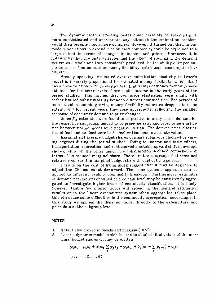
The dynamic factors affecting tastes could certainly be specified in a more sophisticated and appropriate way, although the estimation problem would then become much more complex. However, i t turned out that, in our models, variations in expenditure on each commodity could be explained to a large extent in terms of changes in income and prices. Moreover, i t is noteworthy that the taste variables had the effect of stabilizing the demand system as a whole and they considerably reduced the instability of important parameter estimates, such as money flexibility, subsistence consumption lev- els, etc.

Broadly speaking, estimated average substitution elasticity in Leser's model is inversely proportional to estimated money flexibility, which itself has a close relation to price elasticities. High values of money flexibility were obtained for the lower levels of per capita income in the early years of the period studied. This implies that own price elasticities were small, with rather limited substitutability between different commodities. For periods of more rapid economic growth, money flexibility estimates dropped to some extent, and for recent years they rose appreciably, reflecting the smaller response of consumer demand to price changes.

Since /fit estimates were found to be positive in many cases, demand for the respective subgroups tended to be price-inelastic and cross price elastici- ties between normal goods were negative in sign. The derived price elastici- ties of food and nonfood were both smaller than one in absolute value.

Marginal and average budget shares of many subgroups changed by vary- ing degrees during the period studied. Owing to income and taste effects, transportation, recreation, and rent showed a notable upward shift in average shares, while on the other hand, rice consumption declined remarkably ir, terms of its reduced marginal share. There are few subgroups that remained relatively constant in marginal budget share throughout the period.

Results on the cost of living index suggest that it may be desirable to adjust the CPI somewhat downward. The same systems approach can be applied to different levels of commodity breakdown. Furthermore, estimates of demand parameters obtained at a certain level may be consistently aggre- gated to investigate higher levels of commodity classification. It is likely, however, that a few inferior goods will appear in the demand estimation results or in the linear expenditure system when aggregation takes place; this will cause some difficulties in the commodity aggregation. Accordingly, in this study we applied the dynamic model directly to the expenditure and price data a t the subgroup level.

NOTES

1. This is also proved in Sasaki and Saegusa (1972). 2. Leser's dynamic model, which is used to obtain initial values of the mar-

ginal budget shares bi, may be written

pixi = pi% + a(Gi C p .F -pi%) + bi(m - C pjZj) + cis 3 1

i 1

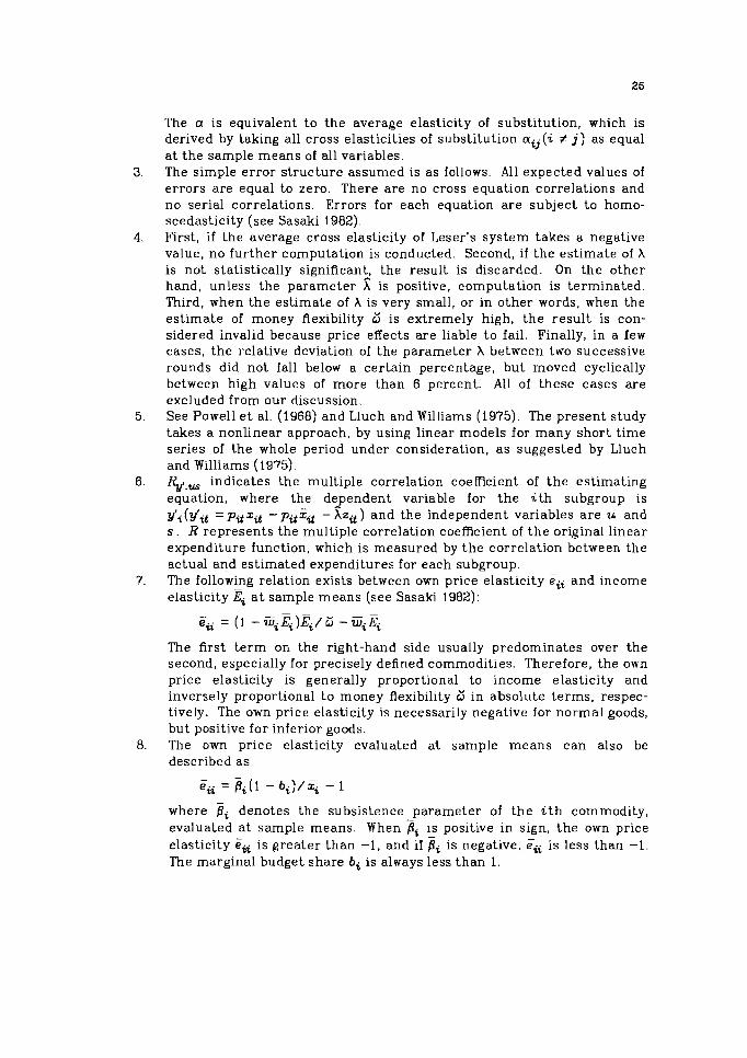
The a is equivalent to the average elasticity of substitution, which is derived by taking all cross elasticities of substitution ai j ( i # j) as equal a t the sample means of all variables.

3. The simple error structure assumed is as follows. All expected values of errors are equal to zero. There are no cross equation correlations and no serial correlations. Errors for each equation are subject to homo- scedasticity (see Sasaki 1982).

4. First, if the average cross elasticity of Leser's system takes a negative value, no further computation is conducted. Second, if the estimate of A is not statistically significant, the result is discarded. On the other hand, unless the parameter is positive, computation is terminated. Third, when the estimate of A is very small, or in other words, when the estimate of money flexibility o' is extremely high, the result is con- sidered invalid because price effects are liable to fail. Finally, in a few cases, the relative deviation of the parameter X between two successive rounds did not fall below a certain percentage, but moved cyclically between high values of more than 6 percent. All of these cases are excluded from our discussion.

5. See Powell e t al. (1968) and Lluch and Williams (1975). The present study takes a nonlinear approach, by using linear models for many short time series of the whole period under consideration, as suggested by Lluch and Williams (1975).

6. Rv,., indicates the multiple correlation coefficient of the estimating equation, where the dependent variable for the i t h subgroup is

A - y'.( ' . = pitz. r. yr.t r.t -pitzit - A z ~ ) and the independent variables are u and s. R represents the multiple correlation coefficient of the original linear expenditure function, which is measured by the correlation between the actual and estimated expenditures for each subgroup.

7. The following relation exists between own price elasticity & and income elasticity Ei a t sample means (see Sasaki 1982):

The first term on the right-hand side usually predominates over the second, especially for precisely defined commodities. Therefore, the own price elasticity is generally proportional to income elasticity and inversely proportional to money flexibility w' in absolute terms, respec- tively. The own price elasticity is necessarily negative for normal goods, but positive for inferior goods.

8. The own price elasticity evaluated a t sample means can also be described as

where pi denotes the subsistence parameter of the i t h commodity, evaluated a t sample means. When Fi is positive in sign, the own price elasticity is greater than -1, and if pi is negative, & is less than -1. The marginal budget share bi is always less than 1.

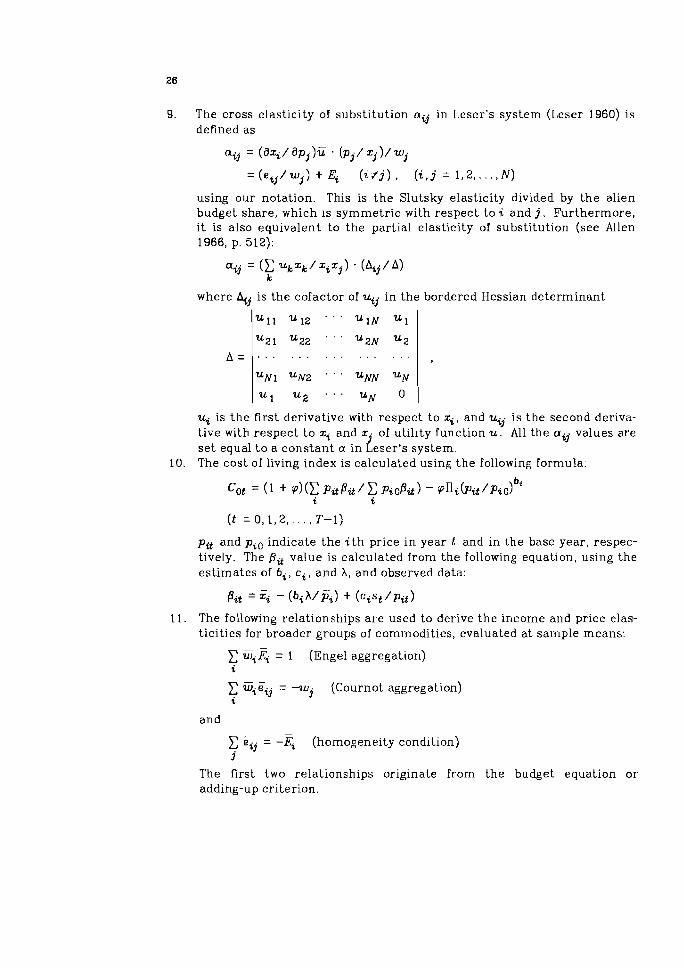
9. The cross elasticity of substitution aij in Leser's system (Leser 1960) is defined as

using our notation. This is the Slutsky elasticity divided by the alien budget share, which is symmetric with respect to i and j. Furthermore, i t is also equivalent to the partial elasticity of substitution (see Allen 1966, p. 512):

where kj is the cofactor of uij in the bordered Hessian determinant

ui is the first derivative with respect to zi, and uij is the second d.eriva- tive with respect to zi and xj of utility function u . All the aij values are set equal to a constant a in Leser's system.

10. The cost of living index is calculated using the following formula:

pit and pic indicate the i t h price in year t and in the base year, respec- tively. The Pit value is calculated from the following equation, using the estimates of bi, ci, and A, and observed data:

Pit = < - (bi U p i ) + (cist / p i t )

11. The following relationships are used to derive the income and price elas- ticities for broader groups of commodities, evaluated at sample means:

C TZiEi = 1 (Engel aggregation) i

-

C vl iqj = -w . (Cournot aggregation) i

3

and -

C Gj = -Ei (homogeneity condition) 3

The first two relationships originate from the budget equation or adding-up criterion.

12. Cross pr ice elast ic i t ies a re confined t o negative values for all pa i rs of commodi t ies provided t h a t bo th marginal budget sha res and subsis tence pa rame te rs a re positive for al l commodit ies. They c a n also be described in t h e form of expressions:

F . . = - b & j a . / ( j i i q ) (i, j = 1,2,, . . , N ; i # j ) t3 3

which are evaluated at sample means . 13. For a detai led discussion see Lluch and Powell (1975). 14. In a n excel lent empir ical study, Yoshihara (1969) f itted Stone's l inear

expendi ture system t o Japanese expendi ture da ta over a long period using a stat ic model.

REFERENCES

Allen, R.G.D. (1966). Mathematical Analysis for Economists. London: The MacMillan Press.

Leser, C.E.V. (1960). Demand functions for nine commodity groups in Australia. Aus- Cralian Journal of S ta t i s t ics , 2 (November): 102-1 13.

Lluch, C. and Powell, LA. (1975). International comparisons of expenditure patterns. h r o p e a n Economic Review, 5 (July): 275-303.

Lluch, C. and Williams, R. (1975). Consumer demand systems and aggregate con- sumption in the USk an application of the extended linear expenditure systeni. Canadian Journal of Economics, 8 (February): 49-66.

Office of the Prime Minister (1950-1980a). Annual Report o n the Consumer Price M e z . Tokyo, Japan.

Office of the Prime Minister (1950-1980b). Annual Report on the Rzmily h c o m e and hkpendi ture Survey. Tokyo, Japan.

Powell, A.A. (1966). A complete system of consumer demand equations for the Aus- tralian economy fitted by a model of additive preferences. Econometrics, 34 (~u ly ) : 66 1-675.

Powell, k A . . Hoa, T.V.. and Wilson, R.H. (1968). A multi-sectoral analysis of consumer demand in the post-war period. Southern Economic Journal, 35 (October): 109-120.

Sasaki. K. and Saegusa. Y. (1972). Food demand functions in linear expenditure sys- tems. Journal of Rural Economics. 44 (June): 20-29.

Sasaki, K. (1982). Est imat ion of the Consumer Demand ,%stem. in Postwar Japan. CP-P2-14. Laxenburg, Austria: International Institute for Applied Systems Analysis.

Yoshihara. K. (1969). Demand functions: an application to the Japanese expenditure pattern. Economet rka , 37 (April): 257-274.

THE AUTHORS

Kozo Sasaki was a Research Scholar with the Food and Agriculture Program a t IIASk He is currently Associate Professor of Socio-Economic Planning a t the Univer- sity of Tsukuba, Sakura, Japan.

Yoshihiro Fukagawa is a systems analyst a t Mathematical Systems Institute. Inc., Tokyo, Japan.