Page 1
DYNAMIC HYBRID CROSS-DOCKING MODEL WITH
MULTIPLE TRUCK TYPES
by
Sitara Holla
A Thesis Presented to the Faculty of the
American University of Sharjah
College of Engineering
in Partial Fulfillment
of the Requirements
for the Degree of
Master of Science in
Engineering Systems Management
Sharjah, United Arab Emirates
May 2015
Page 2
© 2015 Sitara Holla. All rights reserved.
Page 3
Approval Signatures
We, the undersigned, approve the Master’s Thesis of Sitara Holla.
Thesis Title: Dynamic Hybrid Cross-Docking Model with Multiple Truck Types
Signature Date of Signature (dd/mm/yyyy)
___________________________ _______________
Dr. Moncer Hariga
Professor, Engineering Systems Management Graduate Program
Thesis Advisor
___________________________ _______________
Dr. Mehmet Gumus
Associate Professor, Department of Marketing and Information Systems
School of Business Administration
Thesis Co-Advisor
___________________________ _______________
Dr. Rami Afif Asad
Assistant Professor, Industrial Engineering
Thesis Committee Member
___________________________ _______________
Dr. Abdulkadr Dagfous
Professor, Department of Marketing and Information Systems
School of Business Administration
Thesis Committee Member
___________________________ _______________
Dr. Moncer Hariga
Director, Engineering Systems Management Graduate Program
___________________________ _______________
Dr. Mohamed El-Tarhuni
Associate Dean, College of Engineering
___________________________ _______________
Dr. Leland Blank
Dean, College of Engineering
___________________________ _______________
Dr. Khaled Assaleh
Director of Graduate Studies
Page 4
Acknowledgments
Firstly, I would like to express my sincere gratitude to my advisors Dr.
Moncer Hariga and Dr. Mehmet Gumus for their continuous support and guidance,
and for their patience, encouragement, and much required motivation. Their
supervision helped me in the process of researching and writing this thesis and I am
deeply honored to have worked with them for the past two years.
I would also like to express my sincere thanks to the ESM professors who
made my masters experience an inspiring one. They have given us a lot of their time
and knowledge which is greatly appreciated. I would also like to thank American
University of Sharjah, for giving me an opportunity to be a part of this university, to
attend this program, and making it an unforgettable experience.
Page 5
Dedication
This thesis would not have been completed without the continuous support
from my father, mother, husband, brother and grandparents. I dedicate my entire work
to them as they were with me through each and every step of my educational path and
were very supportive when it came to working on the thesis.
I would like to thank my colleagues at L’Oreal, who helped me tremendously
when it came to working on my thesis. I dedicate this work to all my friends and
family as well as those who have supported me and shared the long days and sleepless
nights.
Finally, I dedicate this thesis to all the future ESM students, and I hope these
students would find this thesis helpful in their work and help in seeking knowledge as
well. I also thank God for giving me an opportunity to be a part of this university and
to attend this program, and making this journey a memorable experience.
Page 6
6
Abstract
In today’s business environment, companies are forced to improve their
logistics activities due to high competition. Therefore, improving the design and
operations of distribution networks plays a very important role in efficiently
managing supply chains. Usually, companies operate traditional distribution
networks, which may not be economical for complex networks. Research and practice
have been very inquisitive to find better ways to transport goods across locations. One
way to improve distribution in such networks is through the use of cross-docks, which
are intermediate facilities used to consolidate shipments. This research addressed the
problem of optimizing the flow of goods between multiple supplier and multiple
retailer terminals by taking complete advantage of the concept of hybrid cross-
docking facilities. The objective of the developed model is to determine the best fleet
dispatching and consolidation plans between the terminals using multiple truck types
over a finite planning horizon. The objective function includes quantity dependent
transportation cost components. The model is formulated as a mixed integer linear
program and minimizes the total costs of transportation, throughput and inventory
holding costs over the entire planning horizon. Sensitivity analysis is performed to
assess the effect of varying the problem’s parameters on the model’s outputs. The
results show that as the demand increases, there are more direct shipments using full
truckload (TL) pickups, in order to ensure that the warehouse doesn’t store bulky
products. For large values of inventory holding costs and demand values, there seems
to be little or no inventory of high volumetric weight products left at the warehouse.
Most of the indirect shipments from cross-docks to retailers were for low volume
products using TL trailers. Amongst all input parameters analyzed, changes in
demand had the greatest effect on increasing leasing costs. However, changes in
inventory holding costs were found to have a significant effect on decreasing the
processing costs. Therefore, decision makers have to consider all the studied changes
in parameters at the same time, in order to minimize the total system cost.
Search Terms: Supply Chain, Distribution Network, Logistics, Cross-docking,
Sensitivity Analysis
Page 7
7
Table of Contents
Abstract .......................................................................................................................... 6
List of Figures ................................................................................................................ 8
List of Tables ................................................................................................................. 9
Chapter 1: Introduction ................................................................................................ 10
1.1 Research Objective ............................................................................................. 15
1.2 Research Significance ........................................................................................ 16
1.3 Research Methodology ....................................................................................... 17
1.4 Thesis Outline .................................................................................................... 17
Chapter 2: Literature Review ....................................................................................... 18
2.1 Distribution Systems .......................................................................................... 18
2.2 Warehousing Facility ......................................................................................... 18
2.3 Cross-Docking .................................................................................................... 19
2.4 Cross-Docking Operations ................................................................................. 20
2.5 Types of Cross-Docking..................................................................................... 22
2.6 Cross-Docking Problems.................................................................................... 24
2.6.1 Strategic Decisions. ..................................................................................... 24
2.6.2 Tactical Decisions. ....................................................................................... 25
2.6.3 Operational decisions. ................................................................................. 26
2.6.4 Other related issues. ..................................................................................... 28
2.7 Chapter Summary ............................................................................................... 28
Chapter 3: Model Formulation..................................................................................... 30
3.1 Problem Formulation.......................................................................................... 32
3.2 Illustrative Example ........................................................................................... 37
Chapter 4: Computational Analysis ............................................................................. 53
4.1 Effect of changes in inventory holding cost vs changes in demand ................... 54
4.2 Impacts of leasing costs at medium inventory and medium demand levels. ..... 63
Chapter 5: Conclusion.................................................................................................. 65
5.1 Research findings and key recommendations .................................................... 65
5.2 Limitations and Future Research........................................................................ 67
References .................................................................................................................... 68
Appendix A .................................................................................................................. 72
Appendix B .................................................................................................................. 78
Appendix C .................................................................................................................. 84
Vita ............................................................................................................................... 86
Page 8
8
List of Figures
Figure 1: Pure Cross-Docking Terminal ...................................................................... 12
Figure 2: Hybrid Cross Docking Terminal .................................................................. 13 Figure 3: Cross-Docking Terminal .............................................................................. 22 Figure 4: Quantity Segment for Transportation Function............................................ 31 Figure 5: Proposed network ......................................................................................... 38 Figure 6: Cost comparison study of illustrative examples 1 and 2 .............................. 47
Figure 7: Study on number of trailers and pickups ...................................................... 48 Figure 8: Study on the number of TL and LTL shipments .......................................... 48 Figure 9: Cost comparison of illustrative examples 4 and 5 ........................................ 49 Figure 10: Study on number of trailers and pickups .................................................... 49
Figure 11: Study on number of TL and LTL shipments .............................................. 49 Figure 12: Cost comparison study of illustrative examples 1 and 4 ............................ 50 Figure 13: Study on number of trailers and pickups .................................................... 50
Figure 14: Study on the number of LTL and TL shipments ........................................ 51 Figure 15: Cost comparison study of illustrative examples 2 and 5 ............................ 51 Figure 16: Study on the number of trailers and pickups .............................................. 52 Figure 17: Study on the number of LTL and TL shipments ........................................ 52
Figure 18: Cost structure for scenario 1 ....................................................................... 55 Figure 19: Cost structure for scenario 2 ....................................................................... 56
Figure 20: Cost structure for scenario 3 ....................................................................... 56 Figure 21: Cost structure for scenario 4 ....................................................................... 58
Figure 22: Cost structure for scenario 5 ....................................................................... 58 Figure 23: Cost structure for scenario 6 ....................................................................... 59
Figure 24: Cost structure for scenario 7 ....................................................................... 59 Figure 25: Cost structure for scenario 8 ....................................................................... 60 Figure 26: Cost structure for scenario 9 ....................................................................... 61
Page 9
9
List of Tables
Table 1: Number of variables and constraints for different problem sizes .................. 36
Table 2: List of all model parameters and their values for illustrative example 1 ....... 39 Table 3: Truck parameters for illustrative example 1 .................................................. 40 Table 4: Cut off quantities for segments 1 to 8 for each truck type in all echelons .... 40 Table 5: Cost parameter values for illustrative example 1 .......................................... 40 Table 6: Results of cost structure for illustrative example 1 ....................................... 40
Table 7: Quantity variables for the i-j network using trailers ...................................... 41 Table 8: Quantity variables for the i-j network using pickups ..................................... 42 Table 9: Quantity variables for the j-k network using pickups .................................... 43 Table 10: Total quantity and volume for the j-k network using pickups ..................... 43
Table 11: Trailer and pickups rented for the ij, jk, and ik networks ............................ 43 Table 12: Summary of truck types leased and breakdown of LTL/TL shipments for
illustrative example 1 ................................................................................................... 44
Table 13: Inventory left over at the cross-dock in each period.................................... 44 Table 14: Results of cost structure for illustrative example 2 ..................................... 45 Table 15: Results of cost structure for illustrative example 3 ..................................... 45 Table 16: Results of cost structure for illustrative example 4 ..................................... 46
Table 17: Results of cost structure for illustrative example 5 ..................................... 47 Table 18: List of all the sensitivity parameters and the different performance measures
...................................................................................................................................... 53 Table 19 List of all the sensitivity parameters and the different performance measures
(cont'd) ......................................................................................................................... 54
Page 10
10
Chapter 1: Introduction
Many companies around the world are discovering a powerful source of
competitive advantage through supply chain management (SCM), which comprises all
of the integrated activities and processes that bring a finished product to the market
and create satisfied customers. A supply chain is a system of people, organizations,
information, activities and resources that is involved in helping to move a product or
to deliver a service from the main supplier to the end customer. The end customer
usually gets the finished product that is made from natural resources, raw materials
and other components. SCM encompasses a wide range of topics within it, from
manufacturing operations to purchasing to transportation and physical distribution of
products. It links all of the partners in the supply chain. In addition to these
departments, it also includes a few partners outside the organization such as the
vendors, carriers, information system providers and the third party providers.
Within the organization, the supply chain can be broken down into different
departments such as the physical distribution which encompasses data management,
inbound and outbound transportation, and warehousing and inventory control
activities. Sourcing, procurement, forecasting, production planning and scheduling
and customer service are all part of the supply chain as well. In the recent past,
managers have recognized that getting the products to customers faster than any
competitors will improve the company's competitive position. Companies must seek
new solutions to important supply chain management issues such as distribution
network design, network performance analysis, load planning, and route planning, to
remain competitive. Supply chain management becomes a tool to help achieve
complex strategic corporate objectives. However, sometimes these objectives can be
very conflicting. SCM is a tool to help reduce working capital, accelerate cash to cash
cycles, take assets off the balance sheets, and increase inventory turns.
There are different opportunity areas in supply chain management, and each
has its own benefits. These benefits individually can bring about cost savings and
service enhancements, whereas collectively they can lead to breakthroughs in market
share and profitability. One area of opportunity is distribution network optimization.
Optimizing the distribution network brings about cost advantages. This breaks down
into transportation savings and improvements in inventory carrying costs. Optimizing
Page 11
11
a distribution network usually involves determining the best location for each facility,
selecting the right carriers and setting the proper system configuration. Inventory
management also plays an important role in SCM, and industrial and academic
communities have formed many strategies in order to reduce total inventory cost.
Vendor Managed Inventory (VMI) is one of the most popular strategies in inventory
management. It is a business model in which the buyer of the product gives product
information to the supplier and then the supplier takes full responsibility for
maintaining inventory levels of the product at the buyer’s location of consumption. It
is a very successful concept used by many big box retailers such as Walmart [1]. The
VMI methodology can reduce the demand variability in order to reduce the total
inventory cost. The key to making a VMI work is shared risk.
Another very interesting supply chain initiative that has proven payback
potential is cross-docking. It is the practice of receiving goods and processing them
for distribution to customers in the shortest time possible with minimum handling and
absolutely no storage in the facility. Figure 1 illustrates a pure cross-docking terminal
[1]. This practice brings about potential savings over conventional warehousing. It
uses the concept of consolidation of products from different suppliers intended to be
distributed to one or more retailers. Also since there is no storage, it helps a great deal
in reducing the inventory storage costs. Major retailers like Walmart use cross-
docking to gain a huge competitive advantage over their competitors [1]. They
introduced this concept in their system in the 1980s. It uses staging areas where the
inbound goods are sorted, consolidated and stored until the outbound quantity is
completed for shipment. The storage time is shorter than 24 hours. This strategy has
helped Walmart streamline its supply chain from the point of origin to the point of
sale by not only reducing the handling cost, but also by reducing the operating and
storage costs. To track their sales and inventories, Walmart set up their own satellite
system and is able to reduce unproductive inventories by allowing the stores to
manage their stocks, reducing pack keys across many product categories and ensuring
timely price markdowns.
In practice, there are different types of cross-docking methods used in
industries. Among the different types of cross-docking methods, one of the most
innovative and compromising approaches to cross-docking is the hybrid cross-
Page 12
12
docking method as it provides some degree of storage to supplement the cross-
docking operations.
In this case, the cross-docking terminal has a capacitated warehouse for the
storage of incoming goods that are not shipped the same day. One or more products
stored in the warehouse are blended with the incoming material, and then these
completed palletized orders are loaded on outbound trucks [1]. A slight variation of
this process involves some of the incoming products being routed to temporary
storage at the warehouse while the rest is cross-docked. For the items that are not
shipped immediately, racks are provided near the dock doors to facilitate the
immediate retrieval of items. The hybrid cross-docking model is often used with high
demand and high value products, as well as products that usually require small safety
stock. This approach may also benefit the manufacturer to maintain economic
production volumes while still fulfilling the needs of partners in the downstream
supply chain [1]. Figure 2 illustrates a hybrid cross-docking terminal [1].
Shipment consolidation is another study opportunity in the area of supply
chain. Shippers usually use two ways of transporting items using trucks: one is called
the less-than-truckload shipment (LTL) and the other is called truckload shipment
(TL). The former means that the shipped items do not take up the entire available
Incoming Trucks Outbound Trucks
Receiving Area Pallet Loads Shipping Area
Figure 1: Pure Cross-Docking Terminal
Page 13
13
space on the truck and the latter means that the shipped items would fill up the entire
capacity of the truck.
Shippers who offer TL shipments mainly cater to customers who try to ship in
bulk. Consider an example of a company that has been delivering items from multiple
plants using six different less-than-truckload (LTL) carriers. Through the use of a
third party logistics provider, it will be able to consolidate the multi-vendor lots into
two truckloads. By strategically consolidating the shipments, it helps in cutting the
transportation costs by half. Also it helps reduce inventory levels, cut down on
delivery times, improvise on time delivery, and enhance the product fill rates.
Supplier management is another potential area of study in supply chain management.
It works by involving the supplier during the product design and development stages.
IKEA is one such example, whose furniture comes in simple to assemble kits that
allow them to store the furniture in the same warehouse-like locations where they are
displayed and sold.
Incoming Trucks
Receiving
Area
Outbound Trucks
Shipping Area
Pallet Loads
Warehouse
Storage
Warehouse
Storage
Figure 2: Hybrid Cross Docking Terminal
Page 14
14
Managing transportation in a supply chain is a huge area of concern for both
customers and manufacturers. The parties that are involved are carriers and shippers.
The modes of shipping include road, air, sea, and rail. We specifically look into truck
shipments in this study. The major issues concerning truckload (TL) shipments are
effective utilization of truck space and consistent service among different companies.
The major issues concerning less than truckload (LTL) shipments are location of the
consolidation facilities, vehicle routing and customer service. Shipments could either
be direct from the supplier to customers or indirect through a distribution facility.
Distributors add a lot of value to the supply chain. They bring about economies of
scale in inbound and outbound transportation costs by combining shipments coming
from several manufacturers to the same retailer. They also involve inventory
aggregation at the distributor instead of individual retailer inventories. They also do a
better job in shipment logistics with on time deliveries, shipment tracking and
breaking bulk shipments. There are multiple tradeoffs while considering a
transportation cost reduction. One of them is the tradeoff between transportation,
facility and inventory costs. This usually involves the choice of the transportation
mode and inventory aggregation. Another tradeoff is between transportation costs and
responsiveness. There are many areas of transportation problems that are under study.
One such area is the routing and scheduling in transportation which involves the
assignment of trucks to demand points, sequencing the delivery points, and managing
the exact time of visits/ unloading and loading.
In today’s distribution environment, companies are forced to improve their
logistics and supply chain networks due to high competition. There is a lot of pressure
to manage Stock Keeping Units (SKUs) and have more frequent shipments of fewer
items in less time due to customer demand for better service [2]. Improving
distribution networks plays a very important role in supply chains as it has a huge
impact on inventory reduction. Most companies apply a variety of distribution
networks to transport various types of goods [3]. Most of the goods are transported
from various suppliers to their Distribution Centers (DCs), and then to the retailers
who require that specific good. With increased product proliferation, the average
demand for individual product is decreasing but the variability in individual demand
is increasing [4]. Additionally, logistics costs account for more than 30% of the sales
dollar. Moreover, many companies in different industries (e.g. retail firms and less-
Page 15
15
than-truckload (LTL) logistic providers) look for ways to minimize their total costs by
reducing inventory at every step of the operation, including distribution.
Considering various problems in the area of the supply chain, this study
mainly looks into the area of cross-docking which favors the timely distribution of
freight, better synchronization with demand and a much more efficient usage of
transportation assets. The main advantages involve minimization of warehousing cost
and economies of scale in outbound flows (from the distribution center to the
customers). With this method of distribution, the costly inventory function of a
distribution center becomes minimal, while still sustaining the value-added functions
of consolidation and shipping. Inbound flows are thus directly transferred into
outbound flows in the short term with very little warehouse operations. Shipments
characteristically spend less than 24 hours in the distribution center, sometimes even
less than an hour. With cross-docking, goods are already assigned to a customer, and
hence shipped as a truckload (TL). Cross-docking as a method of distribution that can
be applied to many situations. In the case of manufacturing, it can be used to
consolidate inbound supplies, which can be arranged to support just-in-time (JIT)
assembly (parts for various stages of an assembly line). In the case of distribution, it
can be used to consolidate the products coming from various suppliers and then can
be delivered when the last inbound shipment is received. For transportation, it
involves the consolidation of shipments from several suppliers (often in LTL carriers)
in order to achieve economies of scale with truckload (TL). In the case of retailing,
cross-docking looks into receiving products from multiple suppliers and then sorting
them for outbound shipments to different stores. To date, a lot of research has been
done on cross-docking problems varying from location and layout design of cross-
docks to vehicle routing, dock door assignment and truck scheduling issues to
temporary storage.
1.1 Research Objective
In this research, a supply chain of multiple suppliers providing multiple
product types to multiple retailers is considered. The aim of this research is to
optimize the flow of goods between the supplier-cross dock facility and the cross-
dock facility-retailer terminals. We consider a hybrid cross-docking facility that is
owned by a retailer, who is in charge of transporting these goods between the
terminals. This hybrid facility houses a small capacitated warehouse inventory that is
Page 16
16
required for temporal storage of certain goods. The developed supply chain model
includes the quantity dependent transportation cost component in its objective
function which hasn’t been explored in the supply chain management literature. We
consider both direct and indirect shipments, taking into consideration the capacity of
the warehouse for temporal storage in a cross-docking facility, and also consolidation
at the warehouses and cross-docks. Capacity at the supplier stage, which is specific
for a product type, is considered to be unlimited.
The main aim of this work is to determine the load to be transported from
origin to destination assuming that this load can come from different origins and be
split and consolidated at the warehouses or cross-docks before reaching destinations.
We also consider the availability of trucks which are owned by the retailer. The trucks
are specific to each echelon, meaning they have specific truck types. The retailer can
lease trucks from the market when they are short of their own, and similarly they can
also rent out their trucks to the market to generate rental revenue. Transportation lead
times are considered depending on the route. Also the processing time at the cross-
dock facility is considered to be negligible. The objective is to meet the retailers’
demand with no delays by trying to optimize the flow of goods between terminals and
taking complete advantage of the cross-docking facility. It basically involves finding
out the best fleet dispatching and consolidation plans between the terminals, so as to
minimize the total costs of transportation, throughput and inventory holding costs
over the entire planning horizon, by determining if the load is to be sent directly to
customers or indirectly through cross-docks. The aim of this research is to better
understand the process of hybrid cross-docking and enable a smooth distribution of
products between suppliers and end retailers.
1.2 Research Significance
The main contributions of this research are as follows:
1. Supplement the cross-docking literature with a new model that considers multiple
periods, multiple truck types and non-negative lead times using the concept of
hybrid cross-docking.
2. Formulate the integrated problem as mixed integer linear model.
3. Provide an optimal transportation schedule for fleet dispatching using multiple
truck types (whether using LTL or TL shipment), best consolidation plans at the
cross-dock, and inventory storage decisions at the warehouse.
Page 17
17
4. Assess the impact on cost structure achieved through the integration of the
concept of multiple truck types and a hybrid cross-docking terminal.
1.3 Research Methodology
The following steps will be followed to solve the problem discussed in this
research:
Step 1: Review the literature related to distribution systems, warehousing facilities,
cross-docking, its types and various problems associated with it.
Step 2: Formulate the optimization model by defining the assumptions, objective
function, decision variables, problem parameters and various constraints.
Step 3: Code the formulated model using CPLEX Optimization software.
Step 4: Perform sensitivity analysis to test the effect of the key problem parameters
on the formulated model’s outputs.
1.4 Thesis Outline
Chapter 1 introduced the research problem, the objective, its significance, and
the methodology. Chapter 2 gives a brief introduction on cross-docking, types of
cross-docking, cross-docking problems, and its various applications. Chapter 3 gives a
detailed description of the problem under study. It explains the supply chain network
in detail taking into consideration the quantity segment based transportation cost
function. This chapter also details the mathematical model under consideration with
specific highlights on the costs involved, the decision variables, parameters and
constraints taken into consideration, along with some illustrative examples. Chapter 4
studies the effect of change of various sensitivity parameters on the performance of
the model using various performance measures which are discussed in detail. Chapter
5 gives the results of the sensitivity analysis done on the experimental model taking
various scenarios into consideration, and draws conclusions. The chapter also
discusses the implications of this research on future research.
Page 18
18
Chapter 2: Literature Review
In this chapter, a thorough literature review is performed on the different
distribution systems, with specific focus on cross-docking and its various related
activities. The first part explains cross-docking, its operations and their types. This is
followed by a detailed review of the various strategic and operational problems
involved in cross-docking.
2.1 Distribution Systems
As defined by Chopra [5], “Distribution refers to the steps taken to move and
store a product from the supplier stage to the customer stage in the supply chain.” It
has a direct effect on the supply chain costs and customer experience and therefore
has an impact on the overall profitability of a business. A good distribution strategy
could be used to attain the objectives of a supply chain ranging from high
responsiveness to low cost structure. This is why companies remain vigilant while
selecting a distribution network. This requires decision makers to decide on the
facilities to be built and their locations, such that the network will not just perform
well with the current system state but will serve well for the facility’s lifetime even
when it is being exposed to changing environmental factors and market trends [6].
Facility location decisions are therefore very vital in strategic planning for a wide
variety of firms. Therefore the design and operation of a physical distribution network
involves selecting the best sites for intermediate cross-docking points [7]. Once the
sites have been decided upon, the operations to, from and within the intermediate
cross-docking points have to be optimized.
2.2 Warehousing Facility
Warehouses are physical locations where raw materials, work-in-process
items, or finished products are stored and held as inventory. Companies can take
advantage of the concept of managing a warehouse facility as it helps to meet
increased customer demands, achieve economies of scale, and reduce the lead time
required to deliver products. However, warehousing has some drawbacks. This type
of operation is continuously under pressure to reduce the duration of the stay of
products [8]. The longer the stay, the higher the costs associated with it (i.e. the
inventory holding costs are high). Having a warehouse also introduces other problems
such as opportunity costs, maintenance costs, and obsolescence costs. The major
Page 19
19
functions of warehousing include receiving, putting away, storage, order picking, and
shipping [9].
2.3 Cross-Docking
Cross-docking is defined as a materials handling and distribution strategy in
which the materials flow from receiving to shipping with a primary objective of
eliminating storage, excessive handling, and lead time, and minimizing transportation
and storage costs while also maintaining the level of customer service [10]. It is
basically a way to accelerate the product flow to minimize the lead time from
suppliers to customers [11]. It is also an approach that helps in eliminating inventory
level at the warehouse, as goods are not stored but moved from receiving dock to
shipping dock. Cross-docking enables consolidation of differently-sized shipments to
full truckloads, transported to the same destination, enabling economies in
transportation costs. This is realized from another definition provided by [12]:
“receiving product from a supplier or manufacturer for several end destinations and
consolidating this product with other supplier’s product for common final delivery
destinations.” This implies that products are transported indirectly from suppliers to
retailers via cross-docks as opposed to direct shipment, where the products are
transported directly from suppliers to retailers. It is an intermediate node in a
distribution network that is committed to transshipments of truckloads alone [13]. As
opposed to a warehouse, a cross-dock carries no stock or at least a significantly
reduced amount of stock. In other words, warehouses, now as cross-docks, are
transformed from inventory repositories to points of delivery, consolidation and pick-
up [14, 15]. The focus now shifts from transshipping to not holding stock. This
requires perfect synchronization between the inbound and outbound vehicles, which is
quite difficult to achieve since most of the inbound shipments need to be sorted,
consolidated and stored until the outgoing shipments are completed. This requires
staging procedures. Therefore, cross-docking can be seen from another perspective as
well. It is defined by Van Belle et al. [16] as “the process of consolidating freight with
the same destination (but coming from several origins), with minimal handling and
with little or no storage between unloading and loading of the goods.” If these goods
are to be stored, then it should be for a short period of time of approximately 24 hours
[17, 18, 19].
Page 20
20
In a retail distribution system, for example, the system would receive a single
shipment of a number of truckloads of a given item. This incoming shipment would
be unloaded from the inbound trucks, broken down, and reassembled in outbound
trucks to the stores [10]. This immense application is credited to the fact that cross-
docking improves the flexibility and responsiveness of the supply chain network
while not requiring as much equipment investment as compared to the general
distribution centers. As opposed to the warehousing system, here the vendors would
have a prior request from the customers about the materials they need, such that as
soon as the materials come to the cross-dock they can be transported to the required
destination. The material handling operations of receiving and shipping represent the
physical flow of products. Connected with this is the flow of information concerning
the cross-docked product [4]. For many years, cross-docking has found an immense
level of application in the retail sector. Many large retailers such as Walmart apply
cross-docking which eliminates its inventory holding cost. Mailing companies like
FedEx achieve cost effective transportation and Home Depot ensures transportation
costs are reduced [11]. Therefore, the use of cross-docking operations has resulted in
considerable competitive advantages given the high proportion of distribution costs
for these industries. It shifts focus from “supply” chain to “demand” chain
management [4].
2.4 Cross-Docking Operations
A terminal dedicated for cross-docking, called a “cross-dock”, is usually a
long, narrow rectangle shaped as an I, L, T or X [16]. The working area at a cross-
dock can be classified into an import area and an export area [17]. These are where
breakdown and buildup occur, respectively. Incoming cargo reaches the cross-dock at
various times as they come from a number of suppliers. Cargo are either shipped
directly or sent to the export area where they are loaded into outgoing containers.
Outgoing cargo may then be shipped by vehicles having scheduled departure times,
such as scheduled trains or aircraft. Each incoming (or outgoing) container has a due
date and each outgoing (or incoming) container has a release time.
Generally, the retailer in a supply chain that utilizes cross-docking operations
will place an order to the central office whenever it requires goods [3]. The central
office then collects the orders from all retailers in its vicinity and places a purchase
order (PO) with the respective suppliers. Consequently, suppliers send these
Page 21
21
shipments to intermediate facilities called cross-docking facilities. Suppliers can
either ship a full truckload (TL) or less-than-truckload (LTL) to the cross-dock
facility. However, since suppliers look to minimize transportation costs, they prefer to
fill an entire truckload (TL) rather than sending a less-than-truckload shipment the
entire distance to the cross-docking facility. The cross-docking facility (CF) then
consolidates all cargo going to the same distribution center and fills an outbound truck
which remains docked at the CF until a) the truck has been waiting for a threshold-
hour time window, or b) additional demand arrives for the truck to have a full load,
whichever condition occurs first. Then the load is sent to its destination [3].
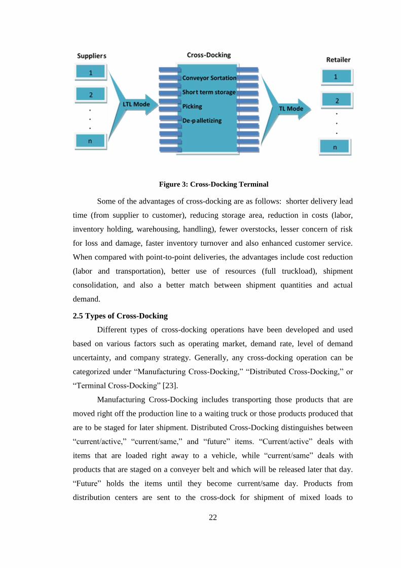
Any cross-docking center can be divided into three areas: loading, sorting, and
unloading areas as shown in Figure 3 [20]. Incoming trucks arriving at the yard of the
cross-dock are directly assigned to a receiving door until and unless all of them are
occupied, then they have to wait in a queue in the yard until assignment. Once they
are docked, supplies (i.e., pallets, packages, or boxes) from the inbound trailer are
unloaded and scanned. All of the supplies contain bar codes which reveal their
identification. In some systems, the goods are also weighed and labeled at the
receiving dock. Then, goods are taken over by a material handling device, such as a
worker operating a fork lift in retail industries, case and pallet conveyors in mail
distribution centers, tilt tray sorters, stretch wrappers, or automated guided vehicle
systems [2, 4]. The goods are then forwarded to the designated shipping door, where
they are loaded onto an outbound truck which serves the designated destination. Once
it is completely loaded, the trailer is removed from the dock and replaced by another
trailer and this course of action repeats.
Cross-docking is usually applied to those companies that deal with huge
volumes of merchandise or the ones that serve a large number of stores [20]. It
handles a high volume of items in a short period of time. There are many advantages
to the cross-docking approach. It streamlines the supply chain operations from the
point of origin to point of sale (POS). The literature provides several advantages of
cross-docking as compared to traditional distribution centers and warehouses and
point-to-point deliveries [13, 21, 22].
Page 22
22
Figure 3: Cross-Docking Terminal
Some of the advantages of cross-docking are as follows: shorter delivery lead
time (from supplier to customer), reducing storage area, reduction in costs (labor,
inventory holding, warehousing, handling), fewer overstocks, lesser concern of risk
for loss and damage, faster inventory turnover and also enhanced customer service.
When compared with point-to-point deliveries, the advantages include cost reduction
(labor and transportation), better use of resources (full truckload), shipment
consolidation, and also a better match between shipment quantities and actual
demand.
2.5 Types of Cross-Docking
Different types of cross-docking operations have been developed and used
based on various factors such as operating market, demand rate, level of demand
uncertainty, and company strategy. Generally, any cross-docking operation can be
categorized under “Manufacturing Cross-Docking,” “Distributed Cross-Docking,” or
“Terminal Cross-Docking” [23].
Manufacturing Cross-Docking includes transporting those products that are
moved right off the production line to a waiting truck or those products produced that
are to be staged for later shipment. Distributed Cross-Docking distinguishes between
“current/active,” “current/same,” and “future” items. “Current/active” deals with
items that are loaded right away to a vehicle, while “current/same” deals with
products that are staged on a conveyer belt and which will be released later that day.
“Future” holds the items until they become current/same day. Products from
distribution centers are sent to the cross-dock for shipment of mixed loads to
Page 23
23
customers. This category falls into Terminal Cross-Docking. Each type of mentioned
cross-docking system should be selected based on different factors such as “Product
Property,” “User Demand,” and “Facility Capacity” [8]. Clearly, not all products are
suitable for cross-docking, not only because of their life cycle and volume but also
because managers prefer to have some safety stock kept in warehouses rather than
utilizing a pure cross-docking approach.
Cross-docking faces many challenges in the distribution environment. These
are not disadvantages, but they are certain issues that any company that is trying to
apply cross-docking in its supply chain has to consider. The factors that influence the
suitability of cross-docking systems are not only the product type and its level of
demand uncertainty, but also other factors such as “Unit Stock-Out Costs” and
“Demand Rate.” “Unit Stock-Out Costs” refers to the cost of lost sales on a single
unit of product, whereas products are categorized from the “Demand Rate”
perspective based on having a “stable and constant demand rate” or an “unstable or
fluctuating demand rate” [4].
Cross-docking would be preferred for items that have low unit stock-out costs
and stable and constant demand. However, cross-docking can still be implemented
even while having a constant demand rate but high stock-out costs. However, care
should be taken with precise planning systems to ensure that the instances of lost sales
are kept to a minimum.
Success of cross-docking operations also depends on equipment and
manpower [4]. Hence, the selection and management of appropriate skilled manpower
and equipment becomes critical to cross-docking operations. In other words, one of
the aims of cross-docking is to minimize required manpower and equipment by
eliminating storing and picking activities. However, material handling at the cross-
docks is quite complicated and labor intensive [10]. Therefore, extra care should be
taken to optimize the personnel requirement to deal with the variety of items handled
by different processes. The layout and design of the receiving and shipping areas are
also major factors for a cross-docking system [4]. A well-designed and well-equipped
dock can process all of the mentioned activities in a faster and more efficient way. In
the cross-docking facility, each carton or pallet from an incoming truck must be
accurately identified at receipt, allocated instantaneously to a purchase order and then
routed to an appropriate outbound door for delivery. The whole process has to be
Page 24
24
done as quickly as possible, which does not leave any room for possible errors.
Therefore, it is also crucial to manage the flow of information as accurately as the
flow of goods. According to [20], one of the concerns of management in cross-
docking should be to design information systems or software to manage and speed up
the cross-docking operations.
2.6 Cross-Docking Problems
Cross-docking practitioners have to deal with many decisions that are to be
made during the design, tactical and operational phase of the cross-docks [16]. These
decisions have to be taken seriously, as they can have a major impact on the
efficiency of the system. The literature gives a brief description of the various cross-
docking decision problems studied. Some of these decisions have an effect on a
longer term; these are known as strategic or tactical decisions. Those that deal with
short term decisions are known as operational decisions. The next section describes
these decisions in detail which have been dealt with in the literature.
2.6.1 Strategic Decisions. This section describes papers that deal with the
strategic assessment of the location of the cross-docks and the best layout for the
cross-docks.
2.6.1.1 Location of cross-docks. The design of a distribution network involves
finding out the location of one or more cross-docks, with a strategic decision to be
made on their position. This problem of locating the cross-docks has attracted a lot of
attention in recent years. Initial studies on the location of cross-docks have been
performed by Sung and Song [24]. The authors found out which of the possible cross-
docks are to be opened and operated and how many vehicles are needed on each arc in
order to minimize the total costs. It assumed consolidation only at one cross-dock. A
similar transportation problem was carried out by Musa, Arnaout, and Jung [14],
where they minimized the total shipping costs by finding out the best way to load and
route the trucks in the network by considering direct shipment as well. Gumus and
Bookbinder [23] studied a similar problem by further taking multiple product types
into consideration. They considered possible consolidation at both manufacturers and
cross-docks; throughput costs at cross-docks were also investigated for multiple types
of products, and the costs for in-transit inventory. They formulated optimization
models to minimize total costs and provide solutions to medium sized networks. A
completely different approach was taken by some other authors [25, 26, 27]. They
Page 25
25
considered a multi-echelon distribution network design problem in which goods (from
multiple product families) had to be transported from the central manufacturing plant
to the different distribution centers, and from there delivered to customers via cross
docks. This problem was solved in two stages, with the first stage focusing on
locating the distribution centers and cross-docks and the second stage deciding the
required quantity of product families that needed to be transported from the plant to
distribution centers and transshipped to cross-docks from warehouses and then
distributed to customers.
2.6.1.2 Layout design. Once the location is known, another strategic decision
that needs to be made is to choose the layout of the cross-dock. A study on this was
conducted by Bartholdi and Gue [28]. They focused on the shape of a cross-dock and
how its shape affected the performance of the cross-dock. They hinted to the fact that
the layout depends on the size of the facility and the pattern of goods flow inside.
Another study on the design of the storage space for temporary storage of incoming
freight was dealt with by Vis and Roodbergen [22]. They suggested that the storage
areas have to be designed with the aim of enabling easy access to the loads and fast
transportation of loads to the loading docks.
2.6.2 Tactical Decisions. Once the cross-dock(s) is (are) available, decisions
have to be made regarding how the goods flow through a network of cross-docks
ensuring supply meeting the demand and minimizing the total costs. This section
describes the papers that dealt with this problem.
2.6.2.1 Cross-docking networks. This research dealt with the determination of
the flow of goods through a network of cross-docks to reduce the costs and make
supply meet demand [16]. Lim et al. [29] focused on extending the transshipment
problem by allowing temporary storage with the aim of minimizing holdover
inventory. This problem assumed that supplier and customer time windows and flow
were constrained by warehouse capacities and transportation schedules. This
transportation is provided by flexible or fixed schedules and lot sizing is handled
through multiple shipments. A similar study was carried out by Chen et al. [15] by
considering a multi-commodity flow problem. Küçükoğlu et al. [30] studied the
cross-docking transportation problem where the products were sent from the suppliers
to customers through the cross-docks without storing them for long time. They
considered two-dimensional truck loading constraints for different sized products to
Page 26
26
find exact capacity of each truck. Buijs et al. [31] presented a new classification
scheme for cross-docking research based on inputs and outputs for each cross-docking
problem aspect.
2.6.3 Operational decisions. This section describes the papers that focus on
the day-to-day decisions to be made in the system. The operational decisions
discussed are that of Vehicle Routing, Dock Door Assignment and Truck Scheduling,
and Temporary Storage.
2.6.3.1 Vehicle routing. The vehicle routing problem deals with the pickup
and delivery processes. The first approaches were taken by [32, 33]. The aim was to
find an optimal vehicle routing schedule for both processes, assuming that all the
pickup vehicles arrive at the cross-dock at the same time so as to prevent waiting
times for the outbound trucks in order to minimize the transportation costs and fixed
costs of the vehicles. Wen et al. [18] explained the vehicle routing problem with
cross-docking (VRPCD), where a homogeneous fleet of vehicles are used to carry
orders from the suppliers to the customers via a cross-dock. The orders are
consolidated at the cross-dock but do not allow intermediate storage. The main
objective is to minimize the overall travel time by respecting the time window
constraints at the centers and a time period for the whole transportation operation.
Ahmadizar et al. [34] studied the cross-docking problem with the aim of assigning
products to suppliers and cross-docks. They optimized the schedules of outbound and
inbound vehicles by minimizing the total costs of purchasing, transportation and
holding costs. Moghadam et al. [35] presented a vehicle routing and scheduling
problem in a network of supplier, customers and cross-docks. They assumed a set of
homogenous vehicles with limited capacities to transfer products between terminals
that must be visited within their time windows.
2.6.3.2 Dock door assignment and truck scheduling. Dock door assignment
problems deal with allocation of each dock door to an inbound or outbound truck
arriving at the cross-dock. Tsui and Chang [36] presented a general model of the dock
door assignment which assumes that all shipments go directly from inbound to
outbound trucks with no storage at the cross-dock. The model also assumed a mid-
term horizon and the designation of strip and stack doors are fixed. This approach
was extended by Cohen and Keren [37], where the model is adapted to allow goods
for a particular destination to be split and delivered to multiple doors allocated to that
Page 27
27
destination. Bartholdi and Gue [38] modeled the travel cost and the three types of
congestion normally experienced in a cross-docking terminal and built a layout to
minimize workers’ travel cost as well as congestion time.
The truck scheduling problem deals with “where” and “when” the trucks
should be processed at the terminal, which consists of assigning the trucks to dock
doors and finding out the docking schedule for all trucks and doors. Some of the
research related to this has been carried out by Yu and Egbelu, and Boysen et al. [20,
39]. They considered settings in which a terminal consists of just a single inbound and
outbound door. Boloori Arabani et al. [40] studied meta-heuristics to find the best
sequence of inbound and outbound trucks, in order to minimize the total operation
time. They dealt with a cross-docking system having temporary storage facility, but
concentrated mainly in establishing coordination between the performances of
inbound and outbound trucks. Alpan et al. [41] dealt with a transshipment scheduling
problem in a multiple dock door cross-docking warehouse, in order to minimize the
sum of inventory holding and truck replacement costs. Lim et al. [16] dealt with the
short-term scheduling problem. They looked into material handling inside the
terminal for a particular truck schedule. Once all the trucks have been docked, all
handling operations have to be assigned to resources in such a way that all operations
at the cross-dock are carried out efficiently. Miao et al. [42] studied scheduling
procedures where trucks are assumed to be given service time windows, which are
maintained as hard constraints. Boysen [43] studied a special truck scheduling
problem covering the requirements of zero inventory cross-docking terminals of the
food industry, dealing with refrigerated products that cannot be stored at cross-docks.
Dondo et al. [44] introduced a new mixed-integer-linear programming formulation for
the vehicle routing problem with cross-docking to find the routing and scheduling of a
mixed fleet, the truck docking sequence, the dock door assignment and the travel time
to move the goods through the cross-dock. Mohtashami et al. [45] proposed a model
that minimizes the make-span, transportation costs and the number of truck trips in
the entire supply chain.
2.6.3.3 Temporary storage. Sometimes due to the imperfect synchronization
of the inbound and outbound vehicles and also because the goods do not arrive in the
same sequence in which they must be loaded, these goods have to be stored in the
cross-docks for a while. Some of the literature dealt with this operational problem of
Page 28
28
where to store the incoming products. An initial study was performed by Vis and
Roodbergen [22], where they found temporary storage locations for the incoming
goods that would minimize the total travel distance of the goods within the cross-
dock. The storage areas have to be designed with the aim of enabling easy access to
the loads and fast transportation of loads to the loading docks. However, they do not
look into any transshipment decisions. Sandal [46] determined which staging strategy
is more suitable for a cross-docking operation as a function of goods attributes and
container-loading requirements. It uses simulation to evaluate many staging strategies
in order to support the optimal loading of the outbound trucks.
2.6.4 Other related issues. Some of the other characteristics are summarized
in the following papers. The loading and unloading procedures are accompanied by a
team of workers and equipment. Lim et al. [17] studied the scheduling of internal
resources for the same, by processing each truck as close as possible to its due date
(Just-In-Time). Yan and Tang [11] analyzed two distinctive cross-docking operations
which are pre-distribution cross-docking operations (Pre-C) and post-distribution
cross-docking operations (Post-C). The differential operational performances are
examined and compared, and they conclude saying that the suitability of Pre-C and
Post-C are sensitive to environmental operational factors such as the uncertainty of
demand, the unit inventory holding cost and storage cost, and unit operation cost at
the cross-dock. Also, Magableh et al. [3] presented a generic simulation model of
cross-docking operations that could be expanded to other cross-docking facilities. It
was used to study the effect of growing demand through the cross-docking facility.
Bellanger et al. [47] worked on optimizing a cross-docking system which is modeled
as a three-stage hybrid flow shop, in which shipments and orders are represented as
batches. They proposed a branch-and-bound algorithm to find a schedule that
minimizes the completion time of the latest batch.
2.7 Chapter Summary
As can be noticed from the preceding literature review, many papers addressed
vehicle routing, truck scheduling, temporary storage, transshipment and other related
operational decisions. But even the papers that addressed temporary storage problems,
they mainly only dealt with staging strategy decisions and truck docking sequences
for cross-docking operations. Yu and Egbelu [20], Borooni Arabani et al. [40] studied
truck scheduling problems by considering a cross-docking system with temporary
Page 29
29
storage. However, they did not consider multiple truck types and any transshipment
decisions. Alpan et al. [41] studied a transshipment scheduling problem in a multi
dock door cross-docking warehouse. However, they did not take multiple product
types into consideration. Even the papers that addressed transshipment problems, did
not consider any temporary storage decisions. Gumus and Bookbinder [23] worked on
a transshipment problem by considering possible consolidation at both manufacturers
and cross-docks, with multiple product types. However they did not consider
transportation lead times and temporary storage decisions. Musa, Arnaout, and Jung
[14] did not take into consideration multiple truck types and storage decisions in their
study. Küçükoğlu et al. [30] studied a transshipment problem, but did not include
direct shipping from suppliers to retailers as well as temporary storage decisions in
their study. Based on the above review of the literature and to the best of our
knowledge, this study is the first to combine the concepts of transshipment and
temporary storage decisions in a cross-docking operation. This study is the first to
address the problem of optimization of the flow of goods between multiple supplier
and multiple retailer terminals, taking complete advantage of a hybrid cross-docking
facility and aiming to find the best fleet dispatching and consolidation plans between
the terminals using multiple truck types over a finite planning horizon. It uses a
quantity-dependent transportation cost component in its objective function which
hasn’t yet been explored in the supply chain management literature.
Page 30
30
Chapter 3: Model Formulation
A supply chain of multiple suppliers providing multiple product types to
multiple retailers is considered. Flow of goods from suppliers to retailers may be
direct or through a number of hybrid cross-docks. The end consumer demand for
each product types is time-varying and realized at the retailers. A retailer owns the
cross-dock facilities and is in charge of transporting goods in the supply chain.
Locations of the cross-dock facilities are known. Each of those facilities incorporates
a small capacitated warehouse used for temporal storage.
There are specific vessel types in the retailers’ fleet, and each vessel type has
its own fixed operating cost per period and fixed capacity. These vessel types differ
and are specific for each echelon, due to the difference in the shipping bulk in each
echelon. The number of vessels owned by the retailer for each vessel type in each
echelon is constant and known. Those numbers cannot be changed as we don’t
consider tactical/strategic decisions. However, if required, the retailer can lease a
vessel from the market in each period at a fixed cost. Similarly, retailers’ idle vessels
in each period are for rent in the market and generate rental revenue. It is to be noted
that the vessels leased from the market and the ones rented to the market differ from
one another and are specific to each echelon.
A number of time periods make up the planning horizon for the retailers’
facility. The demand of each retailer in each period for each product type must be met
by shipments from cross-docks and by direct shipments from the suppliers. There are
also transportation lead times depending on the route. We assume that the lead time
on all routes between suppliers to cross-docks, and between cross-docks and retailers
is the same. Lead time on those routes is regarded as an average value which is
assumed to be the same on both the supplier-cross dock, and cross dock-retailer
network. Lead time for a direct shipment is also assumed to be a fixed time period
independent of the shipment’s origin and destination. Lead times on direct shipment
routes are greater than the lead times on all other routes. We assume that the
processing time at cross-dock facilities is negligible and therefore we do not include it
in this model.
The retailers’ aim is to minimize the total cost of transportation, throughput,
and inventory holding for the entire planning horizon. Holding cost is charged against
Page 31
31
the stock of each product type at the warehouse unit in each period. Throughput cost
is charged against each item that goes through the cross-docking process in each
period.
Transportation cost includes fixed costs and cost of leasing additional trucks
from the market. Fixed cost of transportation is the cost of operating the truck
independent of the route. We apply a quantity-dependent transportation cost function
as shown in Figure 4 for the case of four quantity segments. This transportation
costing is based on real life industry data (in this case, the source is from an
international cosmetic industry) and is approximated to real life data values.
If a retailer orders Q units, then the transportation cost function (considering
any arc) is determined by 𝑐1 (a fixed cost for shipping a small quantity in the first
segment) and then 𝑐2 (fixed cost for shipping a larger quantity in the second segment),
and 𝑦𝑖 (cut off quantities for each segment) as follows:
G (Q) = 𝑐1 , if 0 < 𝑄𝑎𝑛𝑦 𝑎𝑟𝑐𝑤 <𝑦1 and
𝑐2 , if 𝑦1< 𝑄𝑎𝑛𝑦 𝑎𝑟𝑐𝑤 <𝑦2
The cost of maintenance of these trucks is negligible as we assume that the
number of trucks owned is known. Each truck has a weight capacity, and each product
type has a weight used to calculate the total load in a truck. Note that the fixed
operating cost of a truck applies to all trucks whether owned or leased from the
market. Cost of leasing a truck is a separate cost. The unused vehicles of the retailer
can be rented to the market, and the rental revenue generated is deducted from the
Figure 4: Quantity Segment for Transportation Function
Cost
Quantity
𝑌4
𝑌3
𝑌2
𝑌1
𝑐4
𝑐3
𝑐2
𝑐1
∞
Page 32
32
total cost of transportation. The retailer needs to optimize utilizing its own trucks first
before they start renting trucks from the market. Therefore, we assume that revenue
generated by renting a truck to the market is less than the cost of leasing a truck from
the market.
We assume that suppliers have unlimited capacity. Each supplier may offer
multiple product types. We assume that product types offered by a supplier are not
offered by other suppliers in the supply chain. In order to simplify this, we include a
capacity parameter for each supplier which is unlimited for the products offered by
the supplier, and zero for the other product types.
3.1 Problem Formulation
In this section, the decision problem is formulated as a mixed integer linear
program.
Indices
i: supplier zone, (i= 1,2,…,I )
j: cross-dock (j= 1,2,…,J )
k: retailer (k= 1,2,…,K )
l: product type such that l ∈ L, L set of product families
t: time period number (t= 1,2,..,T ), which is in days
a: index for the modified all unit discount segment (a= 1,2,..,A )
Variables
𝑞𝑖𝑗𝑙𝑡: Quantity of product l shipped from supplier i to CD facility j in period t in a
truck
𝑞𝑗𝑘𝑙𝑡: Quantity of product l shipped from CD facility j to retailer k in period t in a
truck
𝑞𝑖𝑘𝑙𝑡 : Quantity of product l shipped from supplier i to retailer k in period t in a truck
𝑅𝑡𝑆𝐶: Number of rented trucks between supplier-cross dock terminals in period t
𝑅𝑡𝐶𝑅: Number of rented trucks between cross dock-retailer terminals in period t
𝑅𝑡𝑆𝑅: Number of rented trucks between supplier-retailer terminals in period t
𝑆𝑖𝑗𝑡𝑎𝑖𝑗
: Binary variable for quantity segment a for arcs i to j in period t
𝑆𝑗𝑘𝑡𝑎𝑗𝑘
: Binary variable for quantity segment a for arcs j to k in period t
𝑆𝑖𝑘𝑡𝑎𝑖𝑘 : Binary variable for quantity segment a for arcs i to k in period t
Page 33
33
𝑇𝑖𝑗𝑡𝑖𝑗
: Number of trucks owned and released by retailer in period t between i-j
𝑇𝑗𝑘𝑡𝑗𝑘
: Number of trucks owned and released by retailer in period t between j-k
𝑇𝑖𝑘𝑡𝑖𝑘 : Number of trucks owned and released by retailer in period t between i-k
𝐻𝑖𝑗𝑡𝑖𝑗
: Number of trucks leased and used specifically in period t between i and j
𝐻𝑗𝑘𝑡𝑗𝑘
: Number of trucks leased and used specifically in period t between j and k
𝐻𝑖𝑘𝑡𝑖𝑘 : Number of trucks leased and used specifically in period t between i and k
𝐼𝑗𝑙𝑡 : Inventory at the CD facility j for product l at the end of period t
Parameters
𝐷𝑘𝑙𝑡: Demand for product l from retailer k in period t
𝑌𝑎𝑖𝑗
: Quantity cut off for segment a in echelon i – j
𝑌𝑎𝑗𝑘
: Quantity cut off for segment a in echelon j - k
𝑌𝑎𝑖𝑘 : Quantity cut off for segment a in echelon i - k
𝑆𝑗𝑙𝑤: Storage capacity of the warehouse unit at facility j for product l in each period
𝑆𝑗𝑙𝑐𝑑: Processing capacity of the cross-docking unit at facility j for product l in each
period
𝑆𝑖𝑙𝑠 : Capacity of supplier i for product l in every period
ℎ𝑗𝑙𝑤 : Inventory holding cost per period for product l at the warehouse unit of CD
facility j
ℎ𝑗𝑙𝑓
: Processing cost for product l at the facility j
𝑤𝑙 : Volumetric weight of product type l
𝐶𝑎𝑖𝑗
: Fixed cost of transporting units in echelon i - j in segment a
𝐶𝑎𝑗𝑘
: Fixed cost of transporting units in the echelon j - k in segment a
𝐶𝑎𝑖𝑘: Fixed cost of transporting units in the echelon i – k in segment a
𝐹𝑖𝑗: Fixed cost of leasing truck specific for echelon i - j from the market in any
period
𝐹𝑗𝑘: Fixed cost of leasing truck specific for echelon j - k from the market in any
period
𝐹𝑖𝑘: Fixed cost of leasing truck specific for echelon i - k from the market in any
period
𝑅𝑖𝑗: Fixed revenue of renting truck from echelon i - j to market in any period.
Page 34
34
𝑅𝑗𝑘: Fixed revenue of renting truck from echelon j - k to market in any period
𝑅𝑖𝑘: Fixed revenue of renting truck from echelon i - k to market in any period
Note that: 𝑅𝑖𝑗 < 𝐹𝑖𝑗 , 𝑅𝑗𝑘 < 𝐹𝑗𝑘 , 𝑅𝑖𝑘 < 𝐹𝑖𝑘
𝐿𝑇𝑖𝑗 : Lead time (in periods) on all arcs i to j
𝐿𝑇𝑖𝑘 : Lead time (in periods) on all arcs j to k
𝐿𝑇𝑖𝑘 : Lead time (in periods) on all arcs i to k
𝑀𝑆𝐶: Total number of trucks owned by retailer for echelon i - j in every period
𝑀𝐶𝑅: Total number of trucks owned by retailer for echelon j - k in every period
𝑀𝑆𝑅: Total number of trucks owned by retailer for echelon i - k in every period
𝑆𝑐𝑎𝑝𝑖𝑗: Capacity of truck specific for echelon i - j
𝑆𝑐𝑎𝑝𝑗𝑘: Capacity of truck specific for echelon j - k
𝑆𝑐𝑎𝑝𝑖𝑘: Capacity of truck specific for echelon i – k
Objective Function
𝑀𝑖𝑛 𝑍 = ∑ ∑ ∑ ∑ 𝑆𝑖𝑗𝑡𝑎𝑖𝑗
𝐶𝑎𝑖𝑗
𝑎𝐽𝑗
𝐼𝑖
𝑇𝑡 + ∑ ∑ ∑ ∑ 𝑆𝑗𝑘𝑡𝑎
𝑗𝑘 𝐶𝑎
𝑗𝑘𝑎
𝐾𝑘
𝐽𝑗
𝑇𝑡 + ∑ ∑ ∑ ∑ 𝑆𝑖𝑘𝑡𝑎
𝑖𝑘 𝐶𝑎𝑖𝑘
𝑎𝐾𝑘
𝐼𝑖
𝑇𝑡 +
∑ ∑ ∑ 𝐻𝑖𝑗𝑡𝑖𝑗
𝐹𝐻𝑖𝑗
𝑇𝑡
𝐽𝑗
𝐼𝑖 + ∑ ∑ ∑ 𝐻𝑗𝑘𝑡
𝑗𝑘𝐹𝐻
𝑗𝑘 𝑇
𝑡𝐾𝑘
𝐽𝑗 + ∑ ∑ ∑ 𝐻𝑖𝑘𝑡
𝑖𝑘 𝐹𝐻𝑖𝑘 𝑇
𝑡𝐾𝑘
𝐼𝑖 + ∑ ∑ ∑ ∑ 𝑞𝑖𝑗𝑙𝑡ℎ𝑗𝑙
𝑓 𝑇
𝑡𝐿𝑙
𝐽𝑗
𝐼𝑖 +
∑ ∑ ∑ 𝐼𝑗𝑙𝑡ℎ𝑗𝑙𝑤𝑇
𝑡𝐿𝑙
𝐽𝑗 − ∑ 𝑅𝑡
𝑖𝑗 𝑅𝑖𝑗𝑇
𝑡 − ∑ 𝑅𝑡𝑗𝑘
𝑅𝑗𝑘𝑇𝑡 − ∑ 𝑅𝑡
𝑖𝑘 𝑅𝑖𝑘𝑇𝑡
The first three cost components capture the fixed cost of transporting units
specific to each echelon in segment a. The next three cost components are the total
cost of leasing trucks from the market which is specific for each echelon. The next
component is the total processing cost of cross-docked items at the cross-docks. The
eighth component is the total cost of goods storage at the warehouse unit of cross-
docks. The last three components are the total revenue generated by renting trucks to
market.
Constraints
1. Total load shipped on each arch i-j, j-k, and i-k in each echelon cannot exceed
the total truck capacity for each echelon-specific truck on those arcs in each
period:
𝑆𝑐𝑎𝑝𝑖𝑗(𝑇𝑖𝑗𝑡𝑖𝑗
+ 𝐻𝑖𝑗𝑡𝑖𝑗
) ≥ ∑ 𝑤𝑙𝑞𝑖𝑗𝑙𝑡𝑙 ∀ 𝑖, 𝑗, 𝑡
𝑆𝑐𝑎𝑝𝑗𝑘(𝑇𝑗𝑘𝑡𝑗𝑘
+ 𝐻𝑗𝑘𝑡𝑗𝑘
) ≥ ∑ 𝑤𝑙𝑞𝑗𝑘𝑙𝑡𝑙 ∀ 𝑗, 𝑘, 𝑡
𝑆𝑐𝑎𝑝𝑖𝑘(𝑇𝑖𝑘𝑡𝑖𝑘 + 𝐻𝑖𝑘𝑡
𝑖𝑘 ) ≥ ∑ 𝑤𝑙𝑞𝑖𝑘𝑙𝑡𝑙 ∀ 𝑖, 𝑘, 𝑡
Page 35
35
2. The retailer owns a fixed number of trucks for each echelon in every period,
whether they are being used or rented to the market:
𝑀𝑆𝐶 = 𝑅𝑡𝑆𝐶 + ∑ ∑ 𝑇𝑖𝑗𝑡
𝑖𝑗𝑖,𝑗
𝑡𝑡−𝐿𝑇𝑖𝑗 ∀ 𝑡
𝑀𝐶𝑅 = 𝑅𝑡𝐶𝑅 + ∑ ∑ 𝑇𝑗𝑘𝑡
𝑗𝑘𝑗,𝑘
𝑡𝑡−𝐿𝑇𝑗𝑘 ∀ 𝑡
𝑀𝑆𝑅 = 𝑅𝑡𝑆𝑅 + ∑ ∑ 𝑇𝑖𝑘𝑡
𝑖𝑘𝑖,𝑘𝑡−𝐿𝑇𝑖𝑘 ∀ 𝑡
3. Retailers’ demand for each product type in each period must be met by direct
shipments from suppliers and indirect shipments from cross-docks:
𝐷𝑘𝑙𝑡 = ∑ 𝑞𝑗𝑘𝑙(𝑡−𝐿𝑇𝑗𝑘)𝐽𝑗 + ∑ 𝑞𝑖𝑘𝑙(𝑡−𝐿𝑇𝑖𝑘)
𝐼𝑖 ∀ 𝑘, 𝑙, 𝑡
4. Inventory balance at the warehouse unit of a CD for each product type:
𝐼𝑗𝑙𝑡 = ∑ 𝑞𝑖𝑗𝑙(𝑡−𝐿𝑇𝑖𝑗)𝐼𝑖 + 𝐼𝑗𝑙(𝑡−1) - ∑ 𝑞𝑗𝑘𝑙𝑡
𝐾𝑘 ∀ 𝑗, 𝑙, 𝑡
5. Warehouse unit has a storage capacity for each product type:
𝐼𝑗𝑙𝑡 ≤ 𝑆𝑗𝑙𝑤 ∀ 𝑗, 𝑙, 𝑡
6. Each CD facility has a cross-docking (processing to prepare shipments)
capacity for shipments directed to retailers:
∑ 𝑞𝑗𝑘𝑙𝑡𝐾𝑘 ≤ 𝑆𝑗𝑙
𝑐𝑑 ∀ 𝑗, 𝑙, 𝑡
7. Each supplier has a capacity for each product type (in applying the model,
infinite capacity for the product types belonging to the supplier, and zero for
the remaining product types), in every period:
∑ 𝑞𝑖𝑗𝑙𝑡𝐽𝑗 + ∑ 𝑞𝑖𝑘𝑙𝑡
𝐾𝑘 ≤ 𝑆𝑖𝑙
𝑠 ∀ 𝑖, 𝑙, 𝑡
8. LTL Shipping Constraints: The quantity transported in each arc lies in one or
more of the quantity segments for the transportation function:
𝑌(𝑎−1)𝑖𝑗
𝑆𝑖𝑗𝑡𝑎𝑖𝑗
≤ ∑ 𝑞𝑖𝑗𝑙𝑡
𝑙
∗ 𝑤𝑙 ≤ ∑ 𝑌𝑎𝑖𝑗
𝑆𝑖𝑗𝑡𝑎𝑖𝑗
𝑎
∀ 𝑖, 𝑗, 𝑡, 𝑎
𝑌(𝑎−1)𝑗𝑘
𝑆𝑗𝑘𝑡𝑎𝑗𝑘
≤ ∑ 𝑞𝑗𝑘𝑙𝑡
𝑙
∗ 𝑤𝑙 ≤ ∑ 𝑌𝑎𝑗𝑘
𝑆𝑗𝑘𝑡𝑎𝑗𝑘
𝑎
∀ 𝑗, 𝑘, 𝑡, 𝑎
𝑌(𝑎−1)𝑖𝑘 𝑆𝑖𝑘𝑡𝑎
𝑖𝑘 ≤ ∑ 𝑞𝑖𝑘𝑙𝑡
𝑙
∗ 𝑤𝑙 ≤ ∑ 𝑌𝑎𝑖𝑘 𝑆𝑖𝑘𝑡𝑎
𝑖𝑘
𝑎
∀ 𝑖, 𝑘, 𝑡, 𝑎
9. Mutually Exclusive Constraint: The quantity transported in each arc should lie
in any one of the segments:
Page 36
36
∑ 𝑆𝑖𝑗𝑡𝑎𝑖𝑗
𝑎
= 1 ∀ 𝑖, 𝑗, 𝑡
∑ 𝑆𝑗𝑘𝑡𝑎𝑗𝑘
𝑎
= 1 ∀ 𝑗, 𝑘, 𝑡
∑ 𝑆𝑖𝑘𝑡𝑎𝑖𝑘
𝑎
= 1 ∀ 𝑖, 𝑘, 𝑡
10. Sign constraints:
𝑆𝑖𝑗𝑡𝑎𝑖𝑗
𝑆𝑗𝑘𝑡𝑎𝑗𝑘
𝑆𝑖𝑘𝑡𝑎𝑖𝑘 – Binary variables
𝑇𝑖𝑗𝑡𝑖𝑗
𝑇𝑗𝑘𝑡𝑗𝑘
𝑇𝑗𝑘𝑡𝑗𝑘
𝐻𝑖𝑗𝑡𝑖𝑗
𝐻𝑗𝑘𝑡𝑗𝑘
𝐻𝑖𝑘𝑡𝑖𝑘 𝑅𝑡
𝑖𝑗 𝑅𝑡
𝑗𝑘 𝑅𝑡
𝑖𝑘 – Integer variables
𝑞𝑖𝑗𝑙𝑡 𝑞𝑗𝑘𝑙𝑡 𝑞𝑖𝑘𝑙𝑡 𝐼𝑗𝑙𝑡 – Continuous variables
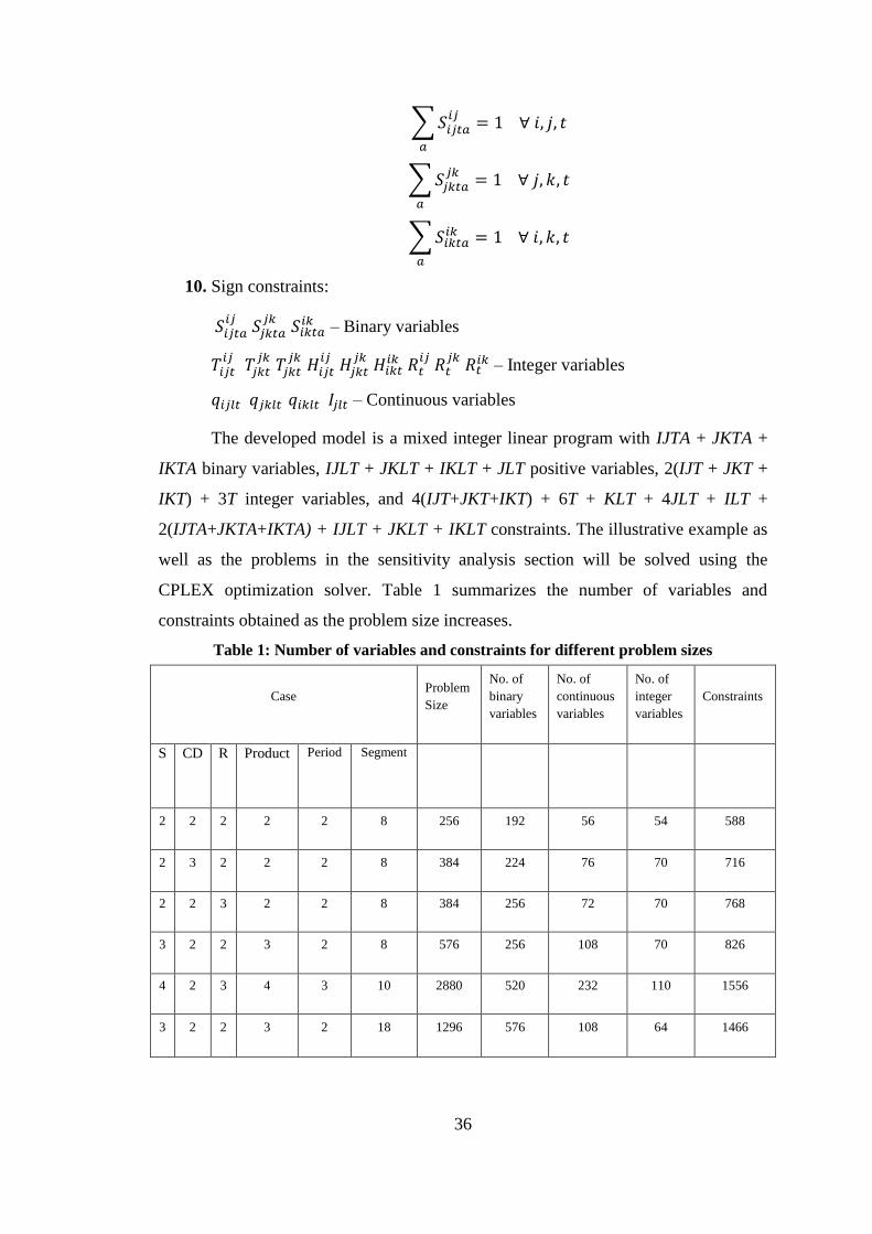
The developed model is a mixed integer linear program with IJTA + JKTA +
IKTA binary variables, IJLT + JKLT + IKLT + JLT positive variables, 2(IJT + JKT +
IKT) + 3T integer variables, and 4(IJT+JKT+IKT) + 6T + KLT + 4JLT + ILT +
2(IJTA+JKTA+IKTA) + IJLT + JKLT + IKLT constraints. The illustrative example as
well as the problems in the sensitivity analysis section will be solved using the
CPLEX optimization solver. Table 1 summarizes the number of variables and
constraints obtained as the problem size increases.
Table 1: Number of variables and constraints for different problem sizes
Case Problem
Size
No. of
binary
variables
No. of
continuous
variables
No. of
integer
variables
Constraints
S CD R Product Period Segment
2 2 2 2 2 8 256 192 56 54 588
2 3 2 2 2 8 384 224 76 70 716
2 2 3 2 2 8 384 256 72 70 768
3 2 2 3 2 8 576 256 108 70 826
4 2 3 4 3 10 2880 520 232 110 1556
3 2 2 3 2 18 1296 576 108 64 1466
Page 37
37
3.2 Illustrative Example
In this section, we consider an example of a local retailer that has its stores
spread across different locations within a country. This retailer owns a hybrid cross-
docking facility which provides some degree of storage to supplement the cross-
docking operations. It offers a variety of products that come from different suppliers.
This retailer may own trucks that are used to transport goods between the supplier and
retailer terminals. There may be cases when they own insufficient trucks or no trucks
at all, and that’s when they can lease trucks from the market for the transportation of
goods. The retailer could also rent out idle trucks to the market and generate revenue.
The main aim of the retailers’ facility is to meet the demand needs of the retailers with
no delays, by trying to optimize the flow of goods between the terminals.
We now assume a supply chain with 2 suppliers, 2 cross-docks and 2 retailers
to illustrate the model developed in the previous section. Figure 5 visualizes the
proposed network for this example. Since each supplier is specific to a particular
product type, in this case we have only two products. The planning horizon covers
two time periods. The cut off quantities for each segment in each echelon are
considered to be different as we consider two different types of trucks used for each
echelon. In this case we consider 8 different segments as listed in the tables below.
The two different types of trucks used are trailers and pickups. The trailer is 13.4m in
length, 2.6m in height and 2.4m in width, around 70m3 in volume. The pickup has a
capacity of 20m3 and is 6.1m in length, 2.5m in height and 2.2m in width. The pallets
considered are standard euro pallets which are 1m3 in size. The various parameters
considered in this model are explained in Tables 2-5 and have been chosen based on
real life industry data (in this case, the source is from an international cosmetic
industry) and are approximated close to the real life data values. The demand is
considered to be uniformly distributed and ranging between 0 to 100 cartons. Each
carton is measured in volumetric weight (m3). The storage capacity of the warehouse
and the processing capacity at the cross-docks are considered to be unlimited. Since
the storage capacity is product-specific, it is measured in terms of the number of
cartons, and so is the processing capacity as well. The weight is defined in terms of
the volumetric weight of a carton of a standard product type, and the size of the carton
depends on the type of product l. In this case we are considering two product types,
each having volumetric weights of 0.1 and 0.2m3. The inventory holding cost is
Page 38
38
charged per m3
per day at the warehouse. Hence, the total inventory cost would be
dependent on the volumetric weights of the products. The processing cost for a
product is the cost of handling a product, and in this case, every time a carton is
picked from the rack or placed back there, there is a handling cost that is charged per
m3
per day. Considering the echelon ij, the fixed cost of transporting 15m3 volume of
products using a trailer, which would classify as the first segment, is considered to be
196 dollars and this would be the cost of a less-than-truckload (LTL) shipment. The
second segment is then followed by an increase of 22 dollars, making it a total of 218
dollars to ship 70m3 volume of products, thereby making it the cost of a truckload
(TL) shipment. The third segment will cost 414 dollars to ship 85m3 volume of
products, and hence will charge for one less than a truckload (LTL) shipment and one
truckload (TL) shipment and so on. The same pattern is followed for the other two
echelons as well. Considering the echelon ij again, the fixed cost of transporting 5m3
volume of products using a pickup, which would classify as the first segment, is
considered to be 125.5 dollars and this would be the cost of a less-than-truckload
(LTL) shipment. The second segment is then followed by an increase of 10.5 dollars,
making it a total of 136 dollars to ship 20m3 volume of products, thereby making it
the cost of a truckload (TL) shipment.
Supplier
s
Cross-docks
Retailers
Inbound trucks
Outbound trucks
Direct shipments
1
1
2 2
1
2
Figure 5: Proposed network
Page 39
39
This will mean that the third segment will cost 261.5 dollars to ship 25m3
volume of products in that segment, and hence will charge for one less than truckload
(LTL) shipment and one truckload (TL) shipment and so on. The same is applicable
for the other two echelons as well. The fixed cost of leasing a truck is dependent on
the ultimate destination and usually the revenue that is generated from renting the
trucks to the market depends on the customer requirement. All costs are reported in
dollars. Here the average lead time for direct shipments is considered to be 1 time
period. The major assumption in this model is that the lead time for indirect shipments
is considered to be less than the time period, and therefore assumed to be zero. The
fixed cost of transporting the units depends on whether a trailer or a pickup is used.
The total number of trucks owned by the retailer for each echelon in every period is
fixed. Also since two types of trucks are available for all echelons, there are two truck
capacities for all echelons. The supplier storage capacity is assumed to be unlimited
for the type of product it supplies. The below Tables 2-5 summarize the values taken
into consideration for all the parameters. We coded the model using GAMS platform
in CPLEX optimization software and ran it on a computer with a 2.1 GHz processor
and 8 GB RAM. Solving each problem took only a few seconds.
Table 2: List of all model parameters and their values for illustrative example 1
Parameter Values
𝐷𝑘𝑙𝑡 (number of cartons) 𝐷111 = 17, 𝐷112 = 84, 𝐷121 = 55, 𝐷122 = 30
𝐷211 = 29, 𝐷212 = 22, 𝐷221 = 35, 𝐷222 = 86
𝑆𝑗𝑙𝑤 (number of cartons) 𝑆11
𝑤 = 5470, 𝑆12𝑤 = 8501
𝑆21𝑤 = 11987, 𝑆22
𝑤 = 19051
𝑆𝑗𝑙𝑐𝑑 (number of cartons) 𝑆11
𝑐𝑑 = 34,734, 𝑆12𝑐𝑑 = 27,868
𝑆21𝑐𝑑 = 8921, 𝑆22
𝑐𝑑 = 24,192
ℎ𝑗𝑙𝑤 ($ per carton per day) 1.36
ℎ𝑗𝑙𝑓
($ per carton) 2.72
𝑤𝑙 (m3) 𝑤1 = 0.1 and 𝑤2= 0.2
𝑆𝑖𝑙𝑠 (number of cartons) Assumed to be large (considered as sum of demand
from each retailer of every product type in every time
period)
Page 40
40
Table 3: Truck parameters for illustrative example 1
Total number of trailers and pickups owned
by the retailer for each echelon in every
period respectively
Truck Capacities of trailer
and pickup respectively
(m3)
Arcs
i-j
3 trailers (period 1) , 3 trailers (period 2)
2 pickups (period 1), 2 pickups (period 2)
Trailer: 70 , Pickup: 20
Arcs
j-k
3 trailers (period 1) , 3 trailers (period 2)
2 pickups (period 1), 2 pickups (period 2)
Trailer: 70 , Pickup: 20
Arcs
i-k
2 trailers (period 1) , 2 trailers (period 2)
2 pickups (period 1), 2 pickups (period 2)
Trailer: 70 , Pickup: 20
Table 4: Cut off quantities for segments 1 to 8 for each truck type in all echelons
Parameter Truck
type
Cut off quantities for segments 1 to 8
𝑌𝑎𝑖𝑗
, 𝑌𝑎𝑗𝑘
, 𝑌𝑎𝑖𝑘 Trailer 15, 70, 85, 140, 155, 210, 225, 280
𝑌𝑎𝑖𝑗
, 𝑌𝑎𝑗𝑘
, 𝑌𝑎𝑖𝑘 Pickup 5, 20, 25, 40, 45, 60, 65, 80
Table 5: Cost parameter values for illustrative example 1
Parameter Fixed cost of transporting units in
segments 1 to 8 using trailer and pickup
respectively
($ per shipment load)
Fixed cost of leasing
truck from market &
Fixed cost of renting
truck to market in any
period ($ per truck)
𝐶𝑎𝑖𝑗
, 𝐶𝑎𝑗𝑘
, 𝐶𝑎𝑖𝑘 Trailer:196,218,414,436,632,654,850,872
Pickup:125.5,136,261.5,272,397.5,408,
533.5,544
Trailer: 485, 435
Pickup: 322, 272
Results
The following results were obtained after running the first case:
Table 6: Results of cost structure for illustrative example 1
Cost Structure
Case
i*j*k*t
Transport
cost ($)
leasing
cost ($)
Inventory
cost ($)
Processing
Cost ($)
Total cost ($)
2*2*2*2 898
0
45.97
153.41
-7331.62
Page 41
41
The first illustrative example resulted in a total cost of $ -7331.62. This
implies that a higher revenue of $ 8429 is generated as compared to the costs incurred.
The tables below summarize the quantity of each product transported in each arc in
every period, and the kind of trucks used for the transportation of products between
echelons. This also gives an understanding of whether a TL or an LTL shipment was
used for the transportation. Illustrative example 1 resulted in no direct shipments
using pickups and no shipments in echelons jk and ik respectively using trailers.
Hence they are not listed in the tables below. The total volume of each product that is
transported from each supplier to each retailer in every period is calculated, which
will help in classifying if the shipment released in that specific arc is a TL or an LTL
shipment. In Table 7, 206 cartons of product 2 were shipped from supplier 2 to cross-
dock 2 in time period 1. Product 2 has a volume of 0.2 m3 and hence the total volume
shipped in that arc is 41.2 m3. Since this lies in the second segment of the
transportation function for the trailers, it is 1 TL shipment.
Table 7: Quantity variables for the i-j network using trailers
i j l t 𝒒𝒊𝒋𝒍𝒕 𝑽𝒊𝒋𝒍𝒕 LTL/TL Shipment
1 1 1 1 0 0
1 1 1 2 0 0
1 1 2 1 0 0
1 1 2 2 0 0
1 2 1 1 0 0
1 2 1 2 0 0
1 2 2 1 0 0
1 2 2 2 0 0
2 1 1 1 0 0
2 1 1 2 0 0
2 1 2 1 0 0
2 1 2 2 0 0
2 2 1 1 0 0
2 2 1 2 0 0
2 2 2 1 206 41.2 1 TL
2 2 2 2 0 0
Page 42
42
As for the network i-j using pickups, 152 cartons of product 1 were shipped
from supplier 1 to retailer 2 in time period 1 (see Table 8). Product 1 has a volume of
0.1 m3 and hence the total volume shipped in that arc is 15.2 m
3. Since this lies in the
second segment of the transportation function for the pickups, it is 1 TL shipment.
Table 8: Quantity variables for the i-j network using pickups
i j l t 𝒒𝟏𝒊𝒋𝒍𝒕 𝑽𝟏𝒊𝒋𝒍𝒕 LTL/TL Shipment
1 1 1 1 0 0
1 1 1 2 0 0
1 1 2 1 0 0
1 1 2 2 0 0
1 2 1 1 152 15.2 1 TL
1 2 1 2 0 0
1 2 2 1 0 0
1 2 2 2 0 0
2 1 1 1 0 0
2 1 1 2 0 0
2 1 2 1 0 0
2 1 2 2 0 0
2 2 1 1 0 0
2 2 1 2 0 0
2 2 2 1 0 0
2 2 2 2 0 0
As for the network j-k using pickups, Table 9 shows the quantities released in
each arc in each time period. Table 10 shows the total volume of products 1 and 2
shipped across to different retailers. In this case it resulted in 4 TL shipments as the
total quantity for each product lies in the second segment of the transportation
function for the pickups. So out of the 16 trailers available, only 1 trailer was used for
transportation in echelon ij, and the rest were rented to the market. Out of the 12
pickups available, 5 pickups (1 in ij and 4 in jk) were used for transportation and the
rest were rented to the market (see Table 11).
Page 43
43
Table 9: Quantity variables for the j-k network using pickups
j k l t 𝒒𝒋𝒌𝒍𝒕 𝑽𝒋𝒌𝒍𝒕
1 1 1 1 0 0
1 1 1 2 0 0
1 1 2 1 0 0
1 1 2 2 0 0
1 2 1 1 0 0
1 2 1 2 0 0
1 2 2 1 0 0
1 2 2 2 0 0
2 1 1 1 17 1.7
2 1 1 2 84 8.4
2 1 2 1 55 11
2 1 2 2 30 6
2 2 1 1 29 2.9
2 2 1 2 22 2.2
2 2 2 1 35 7
2 2 2 2 86 17.2
Table 10: Total quantity and volume for the j-k network using pickups
j k t 𝒒𝟏𝒋𝒌𝒍𝒕 𝑽𝟏𝒋𝒌𝒍𝒕 LTL/TL shipment
2 1 1 72 12.7 1 TL
2 1 2 114 14.4 1 TL
2 2 1 64 9.9 1 TL
2 2 2 108 19.4 1 TL
Table 11: Trailer and pickups rented for the ij, jk, and ik networks
Truck type t 𝑹𝒕𝑺𝑪 𝑹𝒕
𝑪𝑹 𝑹𝒕𝑺𝑹
Trailer 1 2 3 2
2 3 3 2
Pickup 1 1 0 2
2 2 0 2
Page 44
44
The trailer and pickups used in the case study are truckload shipments (TL).
Table 12 shows a breakdown of the TL shipments used for this case.
Table 12: Summary of truck types leased and breakdown of LTL/TL shipments for
illustrative example 1
Truck
type
Total no:
of truck
types
Breakdown of trucks used in
each echelon
LTL/TL shipments
ij jk ik ij jk ik
Trailer 16 1 0 0 1 TL
Pickup 12 1 4 0 1 TL 4 TL
No trucks were leased from the market as the retailer aims at utilizing its own
trucks first, and hence there is no leasing cost incurred. This case resulted in no
direct shipment, all the shipments were indirect, meeting the needs of the retailers’
demands. There is a total of 222 units that is left over as inventory in period 1 and this
is shipped out from the cross-dock in period 2 (see Table 13).
Table 13: Inventory left over at the cross-dock in each period
j l t 𝑰𝒋𝒍𝒕
1 1 1 0
1 1 2 0
1 2 1 0
1 2 2 0
2 1 1 106
2 1 2 0
2 2 1 116
2 2 2 0
In the second illustrative example, the same case as above is considered. We
assume all parameters are the same as the previous illustrative example, with only an
additional assumption that this time the retailer owns no trucks and hence there would
be no trucks rented and only trucks are leased from the market to transport products.
The retailer outsources its transportation function to a third party, and tries to
concentrate on its core competencies like the production, storage and maintenance
activities.
Page 45
45
Results
The following results were obtained after running the second case:
Table 14: Results of cost structure for illustrative example 2
Cost Structure
Case
i*j*k*t
Transport
cost ($)
Leasing
cost ($)
Inventory
cost ($)
Processing
Cost ($)
Total cost ($)
2*2*2*2 898
2095
45.97
153.41
3192.38
This case resulted in a total cost of $3192.38. Since the retailer owns no
trucks, no trucks were rented and hence no revenue was generated. There were a total
of 1 trailer and 5 pickups that were leased for the transportation of products between
the echelons. The trailer was a TL shipment and out of the 5 pickups, there were 4 TL
shipments in arcs jk and 1 TL shipment in arc ij. This case resulted in no direct
shipments; all the shipments were indirect, meeting the needs of the retailers’
demands.
In the third illustrative example, the same base illustrative example is
considered along with the same parameters, but this time we assume that the cut off
quantities for each segment in each echelon is the same as we consider just one type
of truck used for all echelons (in this case we are using trailers only). All the trailers
here are owned by the retailer. We also assume the lead times for direct and indirect
shipments to be negligible, or less than a time period.
Results
This case resulted in a total cost of $ -2038.62. It implies that a higher revenue
of $3480 is generated as compared to the costs incurred. Out of the 14 trailers owned,
2 TL trailers were used in arcs ij, and 4 TL trailers were used in arcs jk. The rest of the
8 trailers were rented to the market.
Table 15: Results of cost structure for illustrative example 3
Cost Structure
Case
i*j*k*t
Transport
cost ($)
Leasing cost
($)
Inventory
cost ($)
Processing
Cost ($)
Total cost
($)
2*2*2*2 1242
0
45.97
153.41
-2038.62
Page 46
46
No trucks were leased from the market as the retailer aims at utilizing its own
trucks first, and hence there is no leasing cost incurred. This case resulted in no direct
shipment, all the shipments were indirect, meeting the needs of the retailers’ demands.
In the fourth illustrative example, the same case as the base illustrative
example is considered along with the same parameters with the only exception: that in
this case, each echelon consists of just one type of truck allotted to it, with echelons ij
and ik allotted to the trailer and echelon jk allotted to the pickups. All the trailers here
are owned by the retailer.
Results
The following results were obtained after running the fourth case:
Table 16: Results of cost structure for illustrative example 4
Cost Structure
Case
i*j*k*t
Transport
cost ($)
Leasing
cost ($)
Inventory
cost ($)
Processing
Cost ($)
Total cost ($)
2*2*2*2 980
0
45.97
153.41
-2300.62
This case resulted in a total cost of $ -2300.62. This means a total revenue of
$3480 was generated. There were a total of 2 TL trailers and 4 TL pickups that were
used for the transportation of products. The rest of the 8 trailers were rented to the
market from all echelons together in periods 1 and 2. However, no pickups were
rented, as all the trucks owned were utilized for the transportation of goods. No trucks
were leased from the market and hence there is no leasing cost incurred. This case
resulted in no direct shipment; all the shipments were indirect, meeting the needs of
the retailers’ demands.
In the last illustrative example, the same case as above is considered with the
only difference being that no trucks are owned by the retailer. The retailer tries to
maximize its core competency operations and hence outsource the transportation
function to a third party. We assume all parameters are the same as the previous
illustrative example.
This case resulted in a total cost of $ 3437.38. Since the retailer owns no
trucks, no trucks were rented and hence no revenue was generated. There were a total
Page 47
47
of 2 TL trailers and 4 TL pickups that were leased for the transportation of products
(Table 17).
Table 17: Results of cost structure for illustrative example 5
Cost Structure
Case
i*j*k*t
Transport
cost ($)
Leasing
cost ($)
Inventory
cost ($)
Processing
Cost ($)
Total cost ($)
2*2*2*2 980
2258
45.97
153.41
3437.38
3.2.1 Analysis of the results of the illustrative examples. The results of the 5
illustrative examples are presented in this section along with explanations regarding
these results. Different performance measures like the cost structure, the total number
of trucks used and the number of LTL and TL shipments were studied and compared
between different cases. It is to be noted that all these cases were run considering low
demand values.
The first study was conducted between the case that owns alternative truck
types for all echelons with a lead time of 1 time period for direct shipments
(illustrative example 1), and the case that has alternative truck types for all echelons
with a lead time of 1 time period for direct shipments and assuming no trucks are
owned (illustrative example 2). Since example 1 rents out the extra trucks owned,
there is a considerable amount of revenue generated and this brings the total cost
down (see Figure 6).
Figure 6: Cost comparison study of illustrative examples 1 and 2
In example 2, there is a considerable amount of leasing cost generated.
However, the revenue generated by renting out trucks in example 1 is much higher
-10000
-5000
0
5000
10000
tottranspcost tothiringcost totproccost totinvcost revenue TotalCost
Cost comparison
Illustrative ex 1 Illustrative ex 2
Page 48
48
than the costs incurred for leasing the trucks in example 2. In this case it is better that
the retailer owns its own trucks. The study on LTL vs. TL shipments (see Figures 7
and 8) shows that mainly TL trailers and TL pickups were used and leased in
examples 1 and 2, respectively.
Figure 7: Study on number of trailers and pickups
Figure 8: Study on the number of TL and LTL shipments
The second study was conducted between the case that owns specific truck
types for each echelon with a lead time of 1 time period for direct shipments
(illustrative example 4), and the case that uses specific truck types for each echelon
with a lead time of 1 time period for direct shipments and assuming no trucks are
owned (illustrative example 5). Since example 4 rents out the extra trucks owned,
there is a considerable amount of revenue generated and this brings the total cost
down (see Figure 9). However, the revenue generated by renting out trucks is not is
not as high as in the case when we had alternative truck types. This revenue does not
really offset the costs incurred by leasing trucks from the market.
0
5
10
15
20
trailers used/leased pickups used/leased trailers rented pickups rented
Trailers vs Pickups
Illustrative ex 1 Illustrative ex 2
0
1
2
3
4
5
LTL trailers TL trailers LTL pickups TL pickups
LTL vs TL shipments
Illustrative ex 1 Illustrative ex 2
Page 49
49
Therefore in this case, it wouldn’t matter if the retailer outsourced its
transportation function to a third party and concentrated instead on its core operational
functions. In this case as well, mainly TL pickups and trailers were used or leased to
transport products (see Figures 10 and 11).
Figure 9: Cost comparison of illustrative examples 4 and 5
Figure 10: Study on number of trailers and pickups
Figure 11: Study on number of TL and LTL shipments
The third study was conducted between the case that has alternative truck
types for all echelons and a lead time of 1 time period for direct shipments
(illustrative example 1), and the case using specific truck types for each echelon and
-4000
-2000
0
2000
4000
tottranspcost tothiringcost totproccost totinvcost revenue TotalCost
Cost comparison
Illustrative ex 4 Illustrative ex 5
0
2
4
6
8
10
trailers used/leased pickups used/leased trailers rented pickups rented
Trailer vs Pickups
Illustrative ex 4 Illustrative ex 5
0
1
2
3
4
5
LTL trailers TL trailers LTL pickups TL pickups
LTL vs TL shipments
Illustrative ex 4 Illustrative ex 5
Page 50
50
having a lead time of 1 time period for direct shipments (illustrative example 4). The
cost of transporting goods for illustrative example 4 is greater and this could perhaps
be due to the limitation of a specific truck type to each echelon (see Figure 12). There
are no pickups rented in example 4 as it has just a few pickups allotted to echelon jk,
and hence utilizes all its pickups. Looking at the LTL vs. TL results, it is better to
have the option of having more pickups, considering low demand values at different
retailers. This allows the consolidation of the goods at the cross-docks and helps in
minimizing the transportation costs. The revenue generated in illustrative example 1 is
much higher than that generated in illustrative example 4. This may be due to the fact
that there are alternative truck types available, which have a higher renting cost for
their transportation. In both cases, we have no LTL trailers or LTL pickups as the
demand is very low (see Figures 13 and 14). The case tries to efficiently use all its
trucks and hence there is maximum usage of TL trailers and pickups.
Figure 12: Cost comparison study of illustrative examples 1 and 4
Figure 13: Study on number of trailers and pickups
-10000
-5000
0
5000
10000
tottranspcost tothiringcost totproccost totinvcost revenue TotalCost
Cost comparison
Illustrative ex 1 Illustrative ex 4
0
2
4
6
8
10
12
14
16
trailers used pickups used trailers rented pickups rented
Trailers vs Pickups
Illustrative ex 1 Illustrative ex 4
Page 51
51
Figure 14: Study on the number of LTL and TL shipments
The fourth study was conducted between the case that has alternative truck
types for all echelons with a lead time of 1 time period for direct shipments and
assuming no trucks are owned (illustrative example 2), and the case that uses specific
truck types for each echelon with a lead time of 1 time period for direct shipments and
assuming no trucks are owned (illustrative example 5). The cost of transporting goods
for illustrative example 5 is greater than that for illustrative example 2 (see Figure
15).
Figure 15: Cost comparison study of illustrative examples 2 and 5
This high cost is attributed to the higher costs of transportation using leased
trailers. The leasing cost is higher for illustrative example 5 because of the limited
availability of multiple truck types in each echelon. Both cases assume no trucks
owned and hence there are no trucks rented to market, thereby generating no revenue.
As seen from the Figures 16 and 17, more pickups than trailers are leased in
illustrative example 5, due to the limited choice available. Looking at the LTL vs TL
results, in both cases we have no LTL trailers and LTL pickups as the demand is very
0
1
2
3
4
5
6
LTL trailers TL trailers LTL pickups TL pickups
LTL vs TL shipment
Illustrative ex 1 Illustrative ex 4
0
1000
2000
3000
4000
tottranspcost tothiringcost totproccost totinvcost revenue TotalCost
Cost comparison
Illustrative ex 2 Illustrative ex 5
Page 52
52
low. The case tries to efficiently use all its trucks and hence there is maximum usage
of TL trailers and pickups.
Figure 16: Study on the number of trailers and pickups
Figure 17: Study on the number of LTL and TL shipments
In the following computational analysis, the case that considers alternative
truck type to each echelon with a lead time of 1 time period for direct shipments and
assuming no trucks are owned is considered as the base case to assess the key
problem parameters in the model’s output. It is more realistic to assume having
alternative truck types, as it brings down the transportation cost due to the availability
of different truck types to cater towards varying demand. The retailer concentrates on
its core competencies. It is also observed from the analysis that there is an impact on
the leasing costs. The leasing costs are lower as compared to the other examples due
to the availability of different truck types. In this case, the pickups cost less than the
trailers.
0
2
4
6
trailers hired pickups hired trailers rented pickups rented
Trailers vs Pickups
Illustrative ex 2 Illustrative ex 5
0
1
2
3
4
5
6
LTL trailers TL trailers LTL pickups TL pickups
LTL vs TL shipments
Illustrative ex 2 Illustrative ex 5
Page 53
53
Chapter 4: Computational Analysis
In this section, we perform a sensitivity analysis to test the effect of varying
the key input problem parameters on the performance of the proposed model’s
outputs. As discussed earlier, the illustrative example with alternative truck types for
each echelon, lead time greater than zero and no trucks owned is taken into
consideration with all the basic parameter values remaining the same.
The various sensitivity parameters that are taken into consideration for the
analysis are the change in demand, the change in inventory holding cost, and change
in leasing cost. The performance of the model along with the changes in the
mentioned sensitivity parameters is studied using the following measures: total cost
structure, total number of trucks used for transportation, the percentage of trucks used
for direct shipment, the percentage of trucks used for indirect shipment, total number
of trucks with TL and LTL shipment, total inventory that goes through the cross-dock,
total number of items processed at the cross-dock, the percentage of inventory over
cross-dock-processed items, percentage of directly shipped quantity over demand,
percentage of total inventory over demand, and the percentage of cross-dock-
processed items over demand. Each scenario is run 10 times in the GAMS platform in
CPLEX optimization software and then the average of each of those above-mentioned
performance measures is taken into consideration to study the effect on the
performance of the model. The various scenarios are discussed in detail in Table 18.
Table 18: List of all the sensitivity parameters and the different performance measures
Scenario# Inventory holding
cost Demand Leasing cost
Time taken
to run
scenario
once
1 L [$1.36]
L [0-100] M [Trailer: $485,
Pickup: $322]
2 seconds
2 L [$1.36] M [100-500] M [Trailer: $485,
Pickup: $322]
48 seconds
3 L [$1.36] H [500-1000] M [Trailer: $485,
Pickup: $322]
16 minutes
Page 54
54
Table 19: List of all the sensitivity parameters and the different performance measures
(cont'd)
4 M [$4.08]
L [0-100] M [Trailer: $485, Pickup:
$322]
2.6 seconds
5 M [$4.08] M [100-500] M [Trailer: $485, Pickup:
$322]
24 seconds
6 M [$4.08] H [500-1000] M [Trailer: $485, Pickup:
$322]
13 minutes
7 H [$8.10]
L [0-100] M [Trailer: $485, Pickup:
$322]
2.8 seconds
8 H [$8.10] M [100-500] M [Trailer: $485, Pickup:
$322]
24 seconds
9 H [$8.10] H [500-1000] M [Trailer: $485, Pickup:
$322]
4.2 minutes
10 M [$4.08] M [100-500] L [$130] for pickup only 15 seconds
11 M [$4.08] M [100-500] M [$220] for pickup only 36 seconds
12 M [$4.08] M [100-500] H [$322] for pickup only 5.6 minutes
13 M [$4.08] M [100-500] L[Trailer: $240
Pickup: $160]
12 seconds
14 M [$4.08] M [100-500] M [Trailer: $485
Pickup: $322]
39 seconds
15 M [$4.08] M [100-500] H [Trailer: $970
Pickup: $644]
1.6 minutes
4.1 Effect of changes in inventory holding cost vs changes in demand
In this section, we study the effect of the change in inventory holding cost on
the performance measures of the model while having low, medium and high demands,
respectively.
4.1.1 Scenario 1 vs. Scenario 2 vs. Scenario 3. The following results were
obtained after running 10 iterations for each of the scenarios. On average, scenario 1
resulted in 98.46% shipments of products 1 and 2 getting processed through the cross-
docks. Out of these total processed items for products 1 and 2, 51.06% of the
inventory was stocked at the capacitated warehouse and shipped the following day.
Less of product 3 was processed and stored at the warehouse. This may be attributed
Page 55
55
to the fact that it has a higher volumetric weight as compared to the other products
and hence most of it is shipped directly using TL pickups, and also because it has a
high demand. Only 3% of product 1 is shipped directly and there was no direct
shipment for product 2. These products were mostly processed through the cross-
docks considering a low inventory holding cost for those items. This resulted in the
consolidation of the products at the cross-docks. The indirect shipments through arcs
ij were mostly using TL pickups and the ones through arcs jk were using TL pickups
and trailers. A total of 5 trailers and 3 pickups were used for the transportation of
products. The total average cost is around $5000. The average cost breakdown is
shown in Figure 18. The processing cost is slightly higher, as 96% of the items are
processed at the cross-dock.
Figure 18: Cost structure for scenario 1
On average, scenario 2 resulted in around 45% of the direct shipments for all
products. This shows that the remaining 55% of products were shipped indirectly. Out
of these total processed items, there was more inventory for product 1 as compared to
product 2 and 3 together, with the inventory over cross-dock-processed ratio at around
9% and 6%, respectively. This may be due to the fact that the volumetric weight of
product 1 is smaller as compared to the other two products and therefore the priority
is in shipping out products 2 and 3, as product 1 will occupy less space in the
warehouse. The indirect shipments used around 12 trailers and 2 pickups and all of
them had a full truckload (TL). This is basically 6 trailers through arcs ij and 6
through jk, and then 1 pickup each on arcs ij and jk, respectively. The total average
cost is around $ 15,000. The cost breakdown is shown in Figure 19. The processing
1441
3246.7
307.306 79.574 0
5074.578
0
1000
2000
3000
4000
5000
6000
tottranspcost tothiringcost totproccost totinvcost revenue TotalCost.l
Cost Structure
Page 56
56
cost is $1091 as only about 55% is processed through the cross-docks.
Figure 19: Cost structure for scenario 2
On average, scenario 3 resulted in around 47% of the direct shipments for all
products. The rest of it was processed through the cross-docks. Out of these total
processed items, there was more inventory for product 1 as compared to products 2
and 3 together, with the inventory over cross-dock-processed ratios at around 7% and
5%, respectively. Again this can be explained by the fact that the volumetric weight of
product 1 is smaller as compared to the other two products and therefore the priority
is in shipping out products 2 and 3. The indirect shipments used around 26 trailers and
2 pickups and all of them used full truckloads (TL). This is basically 13 trailers each
through arcs ij and jk, and then 1 pickup each on arcs ij and jk, respectively. The total
average cost is around $31,000. The cost breakdown is shown in Figure 20.
Figure 20: Cost structure for scenario 3
4.1.2 Scenario 4 vs. Scenario 5 vs. Scenario 6. The following results were
obtained after running 10 iterations for each of the scenarios. On average, scenario 4
4287
9599.4
1091.291 29.921 0
15007.612
0
2000
4000
6000
8000
10000
12000
14000
16000
tottranspcost tothiringcost totproccost totinvcost revenue TotalCost.l
Cost structure
8887.85
19832.9
2431.899 45.804 0
31198.453
0
5000
10000
15000
20000
25000
30000
35000
tottranspcost tothiringcost totproccost totinvcost revenue TotalCost.l
Cost structure
Page 57
57
resulted in only around 12% of the direct shipments for all products, mainly using 1
TL trailer and 1 pickup. This is majorly affected by products 2 and 3, as only 6% of
product 1 is shipped through directly. The remaining products are processed through
the cross-docks. This may be due to low demands. Out of these total processed items,
there was more inventory for product 1 and 2 together as compared to product 3, with
inventory over cross-dock-processed ratio of around 42% and 31%, respectively. As
the inventory costs increases, it is more economical to ship some products directly in
order to minimize the inventory at the warehouse. The indirect shipments used around
5 trailers and 2 pickups, all of them being truckload (TL). This is basically 2 trailers
through arcs ij and 3 trailers through arcs jk, and then 1 pickup each on arcs ij and jk,
respectively. The total average cost is around $5233. The cost breakdown is shown in
Figure 21.
On average, scenario 5 resulted in around 45% of the direct shipments for all
products, mainly using 6 TL trailers and 1 TL pickup. This is majorly affected by
product 3, as only 50% of it is shipped through directly. The remaining products are
processed through the cross-docks. In this case, product 3 has maximum demand as
well, and due to the huge percentage shipped out directly, there is considerably less
inventory at the warehouse. Thus, the inventory is now affected more by products 1
and 2, having around 13% and 7%, respectively. Out of the total demand, an average
of 57.5% of products 1 and 2 are processed at the cross-dock. The indirect shipments
used around 12 trailers and 1 pickup, and all of them, on average, were full truckload
(TL). This is basically 6 trailers through arcs ij and 6 trailers through arcs jk, and then
1 pickup in arc jk, respectively. There were pickups used in arc ij too but they were
very negligible with 10 iterations. Of the 10 iterations run, it was noticed in one of the
runs that an LTL pickup was used in the jk echelon. This could possibly be used for
small deliveries. The total average cost is around $14,458. The cost breakdown is
shown in Figure 22.
On average, scenario 6 resulted in around 49% of the direct shipments for all
products, mainly using 13 TL trailers and 1 and LTL and 1 TL pickup. This is
affected by all products equally. The remaining products are processed through the
cross-docks. However, due to rising inventory holding costs, the priority is in
shipping out the products from the warehouse and hence this scenario results in
around only 2% of inventory for all products combined.
Page 58
58
Figure 21: Cost structure for scenario 4
The indirect shipments used around 13 trailers and 2 pickups and all of them,
on average, had full truckloads (TL). This is basically 6 trailers through arcs ij and 6
trailers through arcs jk, and then 1 pickup in arc jk, respectively. There were pickups
used in arc ij too but they were very negligible with 10 iterations. However, the LTL
pickup used in arc ij could mean that it would be consolidated with other goods from
different suppliers at the cross-dock and then a full TL would be shipped out.
Figure 22: Cost structure for scenario 5
4.1.3 Scenario 7 vs. Scenario 8 vs. Scenario 9. The following results were
obtained after running 10 iterations for each of the scenarios. On average, scenario 7
resulted in 96.4% of the shipments for products 1 and 2 getting processed through the
cross-docks. Out of these total processed items, around 42% of the inventory was
stocked at the capacitated warehouse and shipped the following day or week.
1466.95
3326.2
275.589 165.241 0
5233.982
0
1000
2000
3000
4000
5000
6000
tottranspcost tothiringcost totproccost totinvcost revenue TotalCost.l
Cost Structure
4125.9
9213
1025.82 93.84 0
14458.56
0
2000
4000
6000
8000
10000
12000
14000
16000
tottranspcost tothiringcost totproccost totinvcost revenue TotalCost.l
Cost Structure
Page 59
59
Figure 23: Cost structure for scenario 6
Less of product 3 is stored at the warehouse; this may be attributed to the fact
that it has a higher volumetric weight as compared to the other products and hence
most of it is shipped directly using a TL pickup and TL trailer. Due to the high
inventory holding cost, the priority is to ship out product 3 as it results in high
inventory costs compared to the other two. There were fewer direct shipments for
products 1 and 2 due to a considerably low demand. The indirect shipments through
arcs ij were mostly using 2 TL trailers and 1 TL pickup and the ones through arcs jk
were using 2 TL pickups and 2 TL trailers. A total of 5 trailers and 4 pickups were
used for the transportation of products. The total average cost was around $5154. The
cost breakdown is shown Figure 24.
Figure 24: Cost structure for scenario 7
On average, scenario 8 resulted in around 48% of the direct shipments for all
three products, mainly using 7 TL trailers and 2 TL pickups. This is affected by all
products equally. The remaining products are processed through the cross-docks.
However, due to rising inventory holding costs, there is very little inventory at the
9044.8
20188.3
2440.357 88.618 0
31762.075
0
5000
10000
15000
20000
25000
30000
35000
tottranspcost tothiringcost totproccost totinvcost revenue TotalCost.l
Cost structure
1386.2
3148.1
264.738 355.94 0
5154.976
0
1000
2000
3000
4000
5000
6000
tottranspcost tothiringcost totproccost totinvcost revenue TotalCost.l
Cost structure
Page 60
60
capacitated warehouse. The smallest portion is 1.9% of inventory for product 3 out of
the total 4%, as this is a high volumetric weight product. The indirect shipments used
around 12 trailers and 2 pickups, and all of them, on average, had full truckloads
(TL). This is basically 6 trailers through arcs ij and 6 trailers through arcs jk, and then
1 pickup each in arcs ij and jk, respectively. The total average cost is around $15,450.
The cost breakdown is shown in Figure 25.
Figure 25: Cost structure for scenario 8
On average, scenario 9 resulted in around 49% of the direct shipments for all
products, mainly using 13 TL trailers and 2 TL pickups. This is affected by all
products more or less equally. The remaining products is processed through the cross-
docks. In this case as well, due to the rising inventory holding costs and high demand
for the products, there is no inventory stored for products 2 and 3, and very little
inventory (about 1%) is stored at the warehouse. This means that products 2 and 3 are
processed and shipped out the same day. The indirect shipments used around 26
trailers and 2 pickups and all of them, on average, were full truckload (TL). This is
basically 13 trailers through arcs ij and 13 trailers through arcs jk, and then 1 pickup
each in arcs ij and jk respectively. The total average cost is around $ 32,253. The cost
breakdown is as shown in Figure 26.
4.1.4 Key insights from the analysis. This section describes the insights
drawn from the analysis conducted on the three comparison scenarios mentioned
above. Here, we focus on keeping inventory holding costs constant at low, medium
and high, respectively. The related graphs are presented in Appendix A.
4406.8
9873.7
1049.567 122.645 0
15452.712
0
2000
4000
6000
8000
10000
12000
14000
16000
18000
tottranspcost tothiringcost totproccost totinvcost revenue TotalCost.l
Cost structure
Page 61
61
Figure 26: Cost structure for scenario 9
For low demands, it is observed that there are no direct shipments using
trailers at all. All of the products are shipped through the cross-docks, and this is
mainly done using pickups. However as the demand increases, there is an increased
use of trailers for direct shipments, along with the many pickups used. But the number
of trailers used for direct shipments is not as high as the number of pickups used,
because the model tries to utilize more trailers for the indirect shipments.
As the demand increases, there is a tendency for more high volumetric weight
products to be stored at the warehouse, if they are shipped via cross-docks. Hence the
model tries to avoid this situation for high inventory costs by having direct
movements and hence there is an overall decrease in the number of indirect
shipments. There is a decrease in the number of items being processed at the cross-
dock due to an increase in the number of direct shipments. This is also evident from
the inventory to CD processed ratio, which shows an overall decrease in percentage
with an increase in demand. The indirect shipments are mainly done using TL trailers
as opposed to pickups. It is observed that there is a decrease in the use of pickups in
echelon jk, as more of it is used in the direct shipments.
As the demand increases, it is observed that there is a decrease in the
inventory to CD processed ratio. The model tries to ship out high volumetric weight
products within a day in order to minimize having to store them, as it takes huge
storage space at the warehouse. Therefore there is more direct shipment for such
products and this allows for the storage of low volumetric weight products at the
capitated warehouse. There are relatively high inventory levels for the low volumetric
weight product 1 as compared to products 2 and 3 when the demand is low, but the
9197.2
20542.9
2463.694 49.939 0
32253.733
0
5000
10000
15000
20000
25000
30000
35000
tottranspcost tothiringcost totproccost totinvcost revenue TotalCost.l
Cost structure
Page 62
62
inventory tends to decrease for all items as the demand increases. The inventory is
lowest for product 3 and highest for product 1.
4.1.5 Impacts of inventory costs at the three demand levels. This section
describes the insights drawn from the analysis conducted to study the effect of
varying inventory costs at the three demand levels.
The high volumetric weight goods occupy a lot of storage space at the
warehouse, and this high volume contributes to high inventory costs as the inventory
holding cost increases. So as to avoid the increasing inventory costs, the model tries to
ship out most of the high volumetric weight inventory from the capacitated warehouse
within the same day to different retailers. It is also noticed that a relatively small
percentage of the high volume products as compared to the other products are
processed at the cross-dock and a huge percentage is sent through direct shipments.
The idea here is that, due to the limited storage area at the capacitated warehouse, the
model tries to avoid a simultaneous situation where the warehouse is overstocked with
products as well as a lot of products being processed at the cross-dock. Hence as the
inventory costs increases, it ensures that the high volumetric weight goods are
distributed via both direct and indirect shipments. For example, at low demand level,
100% of product 2 is being processed at the cross-dock and involves no direct
shipment when the inventory holding cost is low. However, as the inventory costs
increase, we can see a gradual decrease to around 85% of products being processed at
the cross-dock, and the rest of around 15% being sent through direct shipment.
Product 3 has 91% of its quantity processed at the cross-dock and around 9% shipped
through directly when the holding costs are low. As the holding costs increases, the
units processed at the cross-dock decrease to around 85%, and the direct shipment
increases to around 15%. In all analyzed cases, major inventory at the cross-dock is
affected by the low volumetric weight of product 1 and scarcity of product 2. This
may be due to the minimal storage space occupied by the products. Therefore the
model tries to retain the low inventory items at the capacitated warehouse and ship out
the high volumetric weight inventory.
As the inventory holding costs increase, there is a need to ship the high
volumetric weight products out of the warehouse immediately so as to reduce the total
inventory costs. This is ensured by the model as it tries to increase the number of
direct shipments. It utilizes more pickups for direct shipments. When we have low
Page 63
63
demand, the model tries to use more pickups as it’s more economical to send a full
truckload of pickups instead of sending LTL trailers for low volumes. Hence in this
case, there is an increase in the utilization of truckload (TL) pickups as compared to
trailers for direct shipments. But for higher demands, there is an increased utilization
of trailers to meet the demand requirements, as more pickups would be used in the
indirect shipments and hence this is compensated by the usage of trailers. But it is
definitely not as high as the usage of pickups for direct shipments. All the trailers and
pickups used for direct shipping are truckload (TL) shipments.
The number of indirect shipments decreases slightly with the increase in
inventory costs, considering an increase in the number of direct shipments. Indirect
shipments mainly ship the low and medium inventory goods through the cross-dock.
The model tries to use a greater number of trailers for indirect shipments (both arcs),
as it tries to consolidate the products at the cross-dock and ship TL trailers to the
retailers. There is, however, an increasing usage of TL pickups in arc jk. This perhaps
could be attributed to the shipping of a truckload of only 1 product type targeted to a
specific retailer. As the inventory holding costs increase, there is a need to lease more
trucks to ship out the inventory from the warehouse and in this case, both echelons
utilize more TL trailers compared to TL pickups.
The model leases more pickups for the direct shipments in order to bring down
the total costs. As the inventory cost increases, fewer high volumetric weight products
are being processed at the warehouse, and therefore this brings down the total
processing costs. Both of these contribute to decreasing the total cost as the inventory
cost increases.
4.2 Impacts of leasing costs at medium inventory and medium demand levels.
This section describes the insights drawn from the analysis conducted to study
the effect of varying leasing costs at medium demand and medium inventory levels.
When the leasing cost for pickup is low, there are more direct shipments
utilizing pickups as compared to trailers. But as leasing costs for pickups increases,
there is a considerable decline in the use of pickups, from 74% to 41%, for the
transportation of products through direct shipment. This is compensated by the
increasing use of trailers for direct shipments. The model thus tries to optimize the use
of pickups, as it is more economical to use a TL trailer by consolidating all products
together rather than using many small pickups to ship the products. This results in less
Page 64
64
volume that is transported through indirect shipments. There is a decreasing number
of trailers used for indirect shipments, especially in echelon jk, and this allows for the
consolidation of products at the cross-dock.
When the leasing costs for both pickup and trailer are low, there is more
utilization of pickups as compared to trailers for direct shipments, considering the fact
that pickups cost less than trailers. This is sufficient to meet the medium demand rate.
But as the leasing cost increases for both the trailers and pickups, it is observed that
there is a decrease in the use of pickups and an increase in the use of trailers for direct
shipments. The model tries to optimize the use of pickups by sending full truckload
trailers as opposed to many small pickups. But it is noticed that when the leasing costs
for both truck types increase to a high value, once again the model tries to bring down
the transportation costs by utilizing more pickups as compared to trailers, as each
trailer costs around 1.5 times that of a pickup. This is compensated by the decreasing
use of trailers for indirect shipments, and a small increase in its usage, when the
leasing costs take a high value. The decrease in the use of pickups for direct
shipments results in rerouting some of the volume through indirect shipments and this
is done using the rest of the pickups especially for echelon jk, which is done by
sending out full TL pickups.
Page 65
65
Chapter 5: Conclusion
This research addressed the cross-docking problem, which is concerned with
determining the best fleet dispatching and consolidation plans between supplier and
retailer terminals using multiple truck types over a finite planning horizon. To the best
of our knowledge, this research was the first to address the problem of optimizing the
flow of multiple products between multiple supplier and retailer terminals taking
complete advantage of a hybrid cross-docking facility. This cross-docking facility
houses a small capacitated warehouse that is required for temporal storage of certain
incoming goods. The developed supply chain model included the quantity-dependent
transportation cost component in its objective function which hasn’t been explored in
the supply chain management literature. Thus the objective is to meet the retailers’
demand with no delays by determining the load to be transported from origin to
destination assuming that this load can come from different origins and be split and
consolidated at the cross-docks before reaching the destinations. The developed
model minimizes the total costs of transportation, throughput and inventory holding
costs over the entire planning horizon. The model was formulated as a mixed integer
linear program and was coded using CPLEX optimization software. The model can be
used to determine the optimal transportation schedule for fleet dispatching using
multiple truck types, whether using LTL or TL shipments, best consolidation plans at
the cross-dock, and inventory storage decisions at the warehouse.
5.1 Research findings and key recommendations
It is observed that as the demand increases, there is an increase in the number
of direct shipments using TL pickups. The model tries to avoid storing high
volumetric weight items at the warehouse, which are responsible for high inventory
costs, by having direct shipments. The indirect shipments are mainly carried out by
TL trailers. Further, the increase in demand was found to have an effect on the
processing costs. Since there is a decrease in the number of some of the medium and
high volumetric weight items being processed at the cross-dock owing to an increase
in the number of direct shipments, this results in decreasing the total processing cost
at the cross-dock. However, there is a huge increase in the leasing costs as demand
increases, as more trailers are leased for indirect shipments. It addition, it is observed
that there is an overall decrease in the inventory to CD processed ratio, as the model
Page 66
66
ensures the priority movements of high volumetric weight items in order to minimize
their storage as it takes huge storage space at the warehouse. It is recommended that
the retailer uses TL pickups for direct shipments as the demand increases, as each
supplier offers specific product types and hence can consolidate all their products in
one TL shipment. For indirect shipments, the facility could use trailers or pickups
depending on the demand of the products required by the retailer. For lower volume
products, the retailer could use pickups and for higher volumes he/she could use
trailers. However, it is recommended that retailers' facility uses more TL trailers for
shipments from cross-docks to retailers in order to allow for consolidation of goods
from different suppliers. This ensures effective utilization of trucks and load space, as
it could store more volume with more than one product type.
Further analysis was carried out to assess the impact of inventory costs at the
three demand levels. As the inventory holding cost increases, it is noticed that a
relatively small percentage of the high volumetric weight products as compared to the
other products are processed at the cross-dock and a huge percentage is sent through
direct shipments. This is attributed to the fact that these products occupy lot of storage
space at the warehouse, and thereby contribute to high inventory costs. In all analyzed
cases, major inventory at the cross-dock is affected by the low volumetric weight
products, possibly due to the reduced space occupied by the products. It is also
observed that there is an increase in the number of direct shipments as the inventory
cost increases, which are mainly done utilizing TL pickups. This direct shipment is
partially helped by the use of TL trailers as the demand increases. Consequently due
to the increase in direct shipments, there is a decrease in the number of indirect
shipments, which focuses on consolidating and shipping the medium and low volume
products using TL trailers and a few TL pickups. Therefore it is recommended that
the retailer aims at minimizing the storage of high volumetric weight products at the
warehouse and aims to ship them out at the earliest as the inventory costs increases. It
would be more economical to send the small percentage of high volumetric weight
products from the cross-docks using a TL trailer than sending two small pickups. So
the model strives to find the best tradeoff between high leasing costs and high
inventory holding costs.
It is noticed that as the leasing costs for the pickups increases, there is a
considerable decline in the use of pickups for the transportation of products through
Page 67
67
direct shipment, which is compensated by the increasing use of trailers. It is more
economical to use a TL trailer by consolidating all products together rather than using
many small pickups to ship the products. The same pattern is followed when the
hiring cost for both the trailers and pickups increases. However, it is noted that as the
leasing costs increase to a high value, again more pickups are utilized for direct
shipments as leasing a trailer is more costly than leasing a pickup. Hence these trailers
would be compensated for indirect shipments at high leasing costs.
5.2 Limitations and Future Research
Whilst the findings of this study could be applied in most cases, there were
some relevant exceptions. Firstly, the size of the network problem solved in this work
is small which restricts the number of suppliers, cross-docks and retailers, over a
small planning horizon. The lead time is considered to be non-negative and we
consider the lead time only for direct shipments which is one time period. This was
used to simplify the work of this study. But a better understanding can be achieved by
studying non-zero lead times for all echelons. We considered a quantity-dependent
transportation function in the objective function. Future research topics could expand
the current study by increasing the size of the problem and expanding the number of
suppliers, cross-docks, and retailers as well as the planning horizon. The development
of heuristic procedures for large problems is another venue for future studies. Further,
future research can also use other types of freight discounts, such as incremental and
all-unit discounts.
Page 68
68
References
[1] R. Kulwiec, "Cross-docking as a supply chain strategy," Target, vol. 20, no. 3,
pp. 28-35, 2004.
[2] M. Rohrer, "Simulation and cross docking," in Proceedings of the 27th
conference on winter simulation, 1995.
[3] G. M. Magableh, M. D. Rossetti and S. Mason, "Modeling and analysis of a
generic cross-docking facility," in Winter Simulation Conference, Orlando,
Florida, 2005.
[4] U. M. Apte and S. Viswanathan, "Effective cross-docking for improving
distribution efficiencies," International Journal of Logistics: Research and
Applications, vol. 3, no. 3, pp. 291-302, 2000.
[5] S. Chopra, "Designing the distribution network in a supply chain,"
Transportation Research Part E: Logistics and Transportation Review, vol. 39,
no. 2, pp. 123-140, 2003.
[6] S. Owen and M. Daskin, "Strategic facility location: A review," European
Journal of Operational Research, vol. 111, no. 3, pp. 423- 447, 1998.
[7] A. Amiri, "Designing a distribution network in a supply chain system:
Formulation and efficient solution procedure," European Journal of Operational
Research, vol. 171, no. 2, pp. 567-576, 2006.
[8] L. Zhengping, M. Y. H. Low, L. Yuan Guan and M. Bin, "Optimal decision-
making on product ranking for crossdocking/warehousing operations," in 6th
IEEE International Conference (INDIN 2008).
[9] D. A. Bodner, T. Govindaraj, K. N. Karathur, N. F. Zerangue and L. F.
McGinnis, "A Process Model and Support Tools for Warehouse Design," in
Proceedings of the 2002 NSF design, service and manufacturing grantees and
research conference, 2002.
[10] Y. Liu and S. Takakuwa, "Simulation-based personnel planning for materials
handling at a cross-docking center under retail distribution environment," in
Proceedings of the 2009 Winter Simulation Conference, 2009.
[11] H. Yan and S. Tang, "Pre-distribution and post-distribution cross-docking
operations," Transportation Research Part E: Logistics and Transportation
Review, vol. 45, no. 6, pp. 843-859, 2009.
[12] E. Kinnear, "Is there any magic in cross docking," Supply Chain Management:
An International Journal, vol. 2, no. 2, pp. 49-52, 1997.
[13] N. Boysen and M. Fliedner, "Cross dock scheduling: Classification, literature
review and research agenda," Omega, vol. 38, no. 6, pp. 413-422, December
2010.
[14] R. Musa, J. Arnaout and H. Hung, "Ant colony optimization algorithm to solve
for the transportation problem of cross-docking network," Computers &
Industrial Engineering, vol. 59, no. 1, pp. 85-92, 2010.
Page 69
69
[15] P. Chen, Y. Guo, A. Lim and B. Rodrigues, "Multiple Crossdocks with Inventory
and Time Windows," Computers & Operations Research, vol. 33, no. 1, pp. 43-
63, 2006.
[16] J. Van Belle, P. Valckenaers and D. Cattrysse, "Cross-docking: State of the art,"
Omega, vol. 40, no. 6, pp. 827-846, 2012.
[17] Y. Li, A. Lim and B. Rodrigues, "Crossdocking—JIT scheduling with time
windows," Journal of the Operational Research Society, vol. 55, no. 12, pp.
1342-1351, 2004.
[18] M. Wen, J. Larsen, J. Clausen, J.-F. Cordeau and G. Laporte, "Vehicle routing
with cross-docking," Journal of the Operational Research Society, vol. 60, no.
12, pp. 1708-1718, 2008.
[19] R. Soltani and S. Sadjadi, "Scheduling trucks in cross-docking systems: A robust
meta-heuristics approach," Transportation Research Part E: Logistics and
Transportation Review, vol. 46, no. 5, pp. 650-666, 2010.
[20] W. Yu and P. Egbelu, "Scheduling of inbound and outbound trucks in cross
docking systems with temporary storage," European Journal of Operational
Research, vol. 184, no. 1, pp. 377-396, 2008.
[21] F. Chen and K. Song, "Minimizing makespan in two-stage hybrid cross docking
scheduling problem," Computers & Operations Research, vol. 36, no. 6, pp.
2066-2073, 2009.
[22] I. Vis and K. Roodbergen, "Positioning of goods in a cross-docking
environment," Computers & Industrial Engineering, vol. 54, no. 3, pp. 677-689,
2008.
[23] M. Gümüş and J. Bookbinder, "Cross-docking and its implications in location-
distribution systems," Journal of Business Logistics, vol. 25, no. 2, pp. 199-228,
2004.
[24] C. S. Song and S. H. Sung, "Integrated service network design for a cross
docking supply chain network," Journal of the Operational Research Society,
vol. 54, no. 12, pp. 1283-1289, 2003.
[25] V. Jayaraman and A. Ross, "A simulated annealing methodology to distribution
network design and management," European Journal of Operational Research,
vol. 144, no. 3, pp. 629-645, 2003.
[26] M. Bachlaus, M. Pandey, C. Mahajan, R. Shankar and M. Tiwari, "Designing an
integrated multi-echelon agile supply chain network: a hybrid taguchi-particle
swarm optimization approach," Journal of Intelligent Manufacturing, vol. 19, no.
6, pp. 747-761, 2008.
[27] A. Ross and V. Jayaraman, "An evaluation of new heuristics for the location of
cross-docks distribution centers in supply chain network design," Computers &
Industrial Engineering, vol. 55, no. 1, pp. 64-79, 2008.
[28] J. J. Bartholdi and K. R. Gue, "The Best Shape for a Cross Dock,"
Transportation Science, vol. 38, no. 2, p. 9, 2004.
[29] A. Lim, Z. Miao, B. Rodrigues and Z. Xu, "Transshipment through crossdocks
Page 70
70
with inventory and time windows," Naval Research Logistics (NRL), vol. 52, no.
8, pp. 724-733, 2005.
[30] I. Küçükoğlu and N. Küçükoğlu, "Simulated Annealing Approach for
Transportation Problem of Cross-docking Network Design," Procedia - Social
and Behavioral Sciences, vol. 109, pp. 1180-1184, 2014.
[31] P. Buijs, I. F. Vis and H. J. Carlo, "Synchronization in cross-docking networks:
A research classification and framework," European Journal of Operational
Research, vol. 239, no. 3, pp. 593-608, 2014.
[32] Y. Lee, J. Jung and K. Lee, "Vehicle routing scheduling for cross-docking in the
supply chain," Computers & Industrial Engineering, vol. 51, no. 2, pp. 247-256,
2006.
[33] C. Liao, Y. Lin and S. Shih, "Vehicle routing with cross-docking in the supply
chain," Expert Systems with Applications, vol. 37, no. 2, pp. 6868-6873, 2010.
[34] F. Ahmadizar, M. Zeynivand and J. Arkat, "Two-level vehicle routing with
cross-docking in a three-echelon supply chain: A genetic algorithm approach,"
Applied Mathematical Modelling, 2015.
[35] S. Shahin Moghadam, S. Fatemi Ghomi and B. Karimi, "Vehicle routing
scheduling problem with cross docking and split deliveries," Computers &
Chemical Engineering, vol. 69, pp. 98-107, 2014.
[36] L. Y. Tsui and C. H. Chang, "A microcomputer based decision support tool for
assigning dock doors in freight yards," Computers & Industrial Engineering, vol.
19, no. 1-4, pp. 309-312, 1990.
[37] Y. Cohen and B. Keren, "Trailer to door assignment in a synchronous cross-dock
operation," International Journal of Logistics Systems and Management, vol. 5,
no. 5, pp. 574-590, 2009.
[38] J. J. Bartholdi and K. R. Gue, "Reducing labor costs in an LTL crossdocking
terminal," Operations Research November/December, vol. 48, no. 6, p. 9, 2000.
[39] N. Boysen, M. Fliedner and A. Scholl, "Scheduling inbound and outbound trucks
at cross docking terminals," OR Spectrum, vol. 32, no. 1, pp. 135-161, 2010.
[40] A. Boloori Arabani, S. Fatemi Ghomi and M. Zandieh, "Meta-heuristics
implementation for scheduling of trucks in a cross-docking system with
temporary storage," Expert Systems with Applications, vol. 38, no. 3, pp. 1964-
1979, 2011.
[41] A. Gulgun, A.-L. Ladier, R. Larbi and B. Penz, "Heuristic solutions for
transshipment problems in a multiple door cross docking warehouse," Computers
& Industrial Engineering, vol. 61, no. 2, pp. 402-408, 2011.
[42] Z. Miao, A. Lim and H. Ma, "Truck dock assignment problem with operational
time constraint within crossdocks," European Journal of Operational Research,
vol. 192, no. 1, pp. 105-115, 2009.
[43] N. Boysen, "Truck scheduling at zero-inventory cross docking terminals,"
Computers & Operations Research, vol. 37, no. 1, pp. 32-41, January 2010.
Page 71
71
[44] R. Dondo and J. Cerdá, "The heterogeneous vehicle routing and truck scheduling
problem in a multi-door cross-dock system," Computers & Chemical
Engineering, vol. 76, pp. 42-62, 2015.
[45] A. Mohtashami, M. Tavana, F. J. Santos-Arteaga and A. Fallahian-Najafabadi,
"A novel multi-objective meta-heuristic model for solving cross-docking
scheduling problems," Applied Soft Computing, vol. 31, pp. 30-47, 2015.
[46] S. Sandal, "Staging approaches to reduce overall cost in a cross dock
environment," Masters, Industrial engineering, University of Missouri,
Columbia, 2005.
[47] A. Bellanger, S. Hanafi and C. Wilbaut, "Three-stage hybrid-flowshop model for
cross-docking," Computers & Operations Research, vol. 40, no. 4, pp. 1109-
1121, 2013.
[48] I. F. A. Vis and K. J. Roodbergen, "Layout and control policies for cross docking
operations," Computers & Industrial Engineering, vol. 61, no. 4, pp. 911-919,
Nov 2011.
[49] F. A. Santos, G. R. Mateus and A. S. da Cunha, "The Pickup and Delivery
Problem with Cross-Docking," Computers & Operations Research, vol. 40, no.
4, pp. 1085-1093, 2013.
Page 72
72
Appendix A
Study of the various sensitivity parameters with increasing demand values, at
low inventory holding cost
0
5000
10000
15000
20000
25000
30000
35000
tottranspcost tothiringcost totproccost totinvcost revenue TotalCost.l
Cost comparison
Scenario 1 Scenario 2 Scenario 3
0102030405060
Direct vs Indirect
Scenario 1 Scenario 2 Scenario 3
0
2
4
6
8
10
12
14
LTL vs TL Shipments
Scenario 1 Scenario 2 Scenario 3
Page 73
73
Study of the various sensitivity parameters with increasing demand values, at
low inventory holding cost
0
10
20
30
40
50
60
inv/processed pdt 1 inv/processed pdt 2 inv/processed pdt 3
Inventory/CD processed ratio
Scenario 1 Scenario 2 Scenario 3
0
10
20
30
40
50
60
inv/demand pdt 1 inv/demand pdt 2 inv/demand pdt 3
Inventory/Demand ratio
Scenario 1 Scenario 2 Scenario 3
0
20
40
60
80
100
120
processed/demand pdt 1 processed/demand pdt 2 processed/demand pdt 3
CD processed/Demand ratio
Scenario 1 Scenario 2 Scenario 3
Page 74
74
Study of the various sensitivity parameters with increasing demand values, at
medium inventory holding cost
0
5000
10000
15000
20000
25000
30000
35000
tottranspcost tothiringcost totproccost totinvcost revenue TotalCost.l
Cost comparison
Scenario 4 Scenario 5 Scenario 6
0102030405060
Direct vs Indirect
Scenario 4 Scenario 5 Scenario 6
0
2
4
6
8
10
12
14
LTL vs TL shipment
Scenario 4 Scenario 5 Scenario 6
Page 75
75
Study of the various sensitivity parameters with increasing demand values, at
medium inventory holding cost
0
10
20
30
40
50
60
inv/processed pdt 1 inv/processed pdt 2 inv/processed pdt 3
Inventory/CD processed ratio
Scenario 4 Scenario 5 Scenario 6
0
10
20
30
40
50
inv/demand pdt 1 inv/demand pdt 2 inv/demand pdt 3
Inventory/Demand ratio
Scenario 4 Scenario 5 Scenario 6
0
20
40
60
80
100
processed/demand pdt 1 processed/demand pdt 2 processed/demand pdt 3
CD processed/Demand ratio
Scenario 4 Scenario 5 Scenario 6
Page 76
76
Study of the various sensitivity parameters with increasing demand values, at
high inventory holding cost
0
5000
10000
15000
20000
25000
30000
35000
tottranspcost tothiringcost totproccost totinvcost revenue TotalCost.l
Cost comparison
Scenario 7 Scenario 8 Scenario 9
0
10
20
30
40
50
60
Directtrailer Indirecttrailer Indirecttrailer1 Directpickup Indirectpickup Indirectpickup1
Direct vs Indirect
Scenario 7 Scenario 8 Scenario 9
02468
10121416
LTL vs TL shipment
Scenario 7 Scenario 8 Scenario 9
Page 77
77
Study of the various sensitivity parameters with increasing demand values, at
high inventory holding cost
0
10
20
30
40
50
60
inv/processed pdt 1 inv/processed pdt 2 inv/processed pdt 3
Inventory/CD processed ratio
Scenario 7 Scenario 8 Scenario 9
0
10
20
30
40
50
60
inv/demand pdt 1 inv/demand pdt 2 inv/demand pdt 3
Inventory/Demand ratio
Scenario 7 Scenario 8 Scenario 9
0
20
40
60
80
100
120
processed/demand pdt 1 processed/demand pdt 2 processed/demand pdt 3
CD processed/Demand ratio
Scenario 7 Scenario 8 Scenario 9
Page 78
78
Appendix B
Study of the various sensitivity parameters with increasing inventory costs, at
low demand values
0
1000
2000
3000
4000
5000
6000
tottranspcost tothiringcost totproccost totinvcost revenue TotalCost.l
Cost comparison
Scenario 1 Scenario 4 Scenario 7
0102030405060
Direct vs Indirect
Scenario 1 Scenario 4 Scenario 7
00.5
11.5
22.5
33.5
LTL vs TL shipment
Scenario 1 Scenario 4 Scenario 7
Page 79
79
Study of the various sensitivity parameters with increasing inventory costs, at
low demand values
0
10
20
30
40
50
60
inv/processed pdt 1 inv/processed pdt 2 inv/processed pdt 3
Inventory/CD processed ratio
Scenario 1 Scenario 4 Scenario 7
0
10
20
30
40
50
60
inv/demand pdt 1 inv/demand pdt 2 inv/demand pdt 3
Inventory/Demand ratio
Scenario 1 Scenario 4 Scenario 7
75
80
85
90
95
100
105
processed/demand pdt 1 processed/demand pdt 2 processed/demand pdt 3
CD processed/Demand ratio
Scenario 1 Scenario 4 Scenario 7
Page 80
80
Study of the various sensitivity parameters with increasing inventory costs, at
medium demand values
0
5000
10000
15000
20000
tottranspcost tothiringcost totproccost totinvcost revenue TotalCost.l
Cost comparison
Scenario 2 Scenario 5 Scenario 8
0
10
20
30
40
50
60
Directtrailer Indirecttrailer Indirecttrailer1 Directpickup Indirectpickup Indirectpickup1
Direct vs Indirect
Scenario 2 Scenario 5 Scenario 8
0
1
2
3
4
5
6
7
LTL vs TL shipment
Scenario 2 Scenario 5 Scenario 8
Page 81
81
Study of the various sensitivity parameters with increasing inventory costs, at
medium demand values
0
2
4
6
8
10
12
14
16
inv/processed pdt 1 inv/processed pdt 2 inv/processed pdt 3
Inventory/CD processed ratio
Scenario 2 Scenario 5 Scenario 8
0
2
4
6
8
10
inv/demand pdt 1 inv/demand pdt 2 inv/demand pdt 3
Inventory/Demand ratio
Scenario 2 Scenario 5 Scenario 8
44
46
48
50
52
54
56
58
60
processed/demand pdt 1 processed/demand pdt 2 processed/demand pdt 3
CD processed/Demand ratio
Scenario 2 Scenario 5 Scenario 8
Page 82
82
Study of the various sensitivity parameters with increasing inventory costs, at
high demand values
0
5000
10000
15000
20000
25000
30000
35000
tottranspcost tothiringcost totproccost totinvcost revenue TotalCost.l
Cost comparison
Scenario 3 Scenario 6 Scenario 9
05
1015202530354045
Direct vs Indirect
Scenario 3 Scenario 6 Scenario 9
0
2
4
6
8
10
12
14
16
LTL vs TL shipment
Scenario 3 Scenario 6 Scenario 9
Page 83
83
Study of the various sensitivity parameters with increasing inventory costs, at
high demand values
0
1
2
3
4
5
6
7
8
inv/processed pdt 1 inv/processed pdt 2 inv/processed pdt 3
Inventory/CD processed ratio
Scenario 3 Scenario 6 Scenario 9
0
0.5
1
1.5
2
2.5
3
3.5
4
4.5
inv/demand pdt 1 inv/demand pdt 2 inv/demand pdt 3
Inventory/Demand ratio
Scenario 3 Scenario 6 Scenario 9
46
47
48
49
50
51
52
53
54
55
56
processed/demand pdt 1 processed/demand pdt 2 processed/demand pdt 3
CD processsed/Demand ratio
Scenario 3 Scenario 6 Scenario 9
Page 84
84
Appendix C Study of the various sensitivity parameters with increasing leasing costs for
pickups, at medium demand values and medium inventory costs
0
5000
10000
15000
20000
tottranspcost tothiringcost totproccost totinvcost revenue TotalCost.l
Cost comparison
Scenario 11 Scenario 12 Scenario 13
01020304050607080
Direct vs Indirect
Scenario 11 Scenario 12 Scenario 13
02468
10121416
LTL vs TL shipment
Scenario 11 Scneario 12 Scenario 13
Page 85
85
Study of the various sensitivity parameters with increasing leasing costs for
pickups and trailers, at medium demand values and medium inventory costs
05000
1000015000200002500030000
Cost comparison
Scenario 14 Scenario 15 Scenario 16
01020304050607080
Direct vs Indirect
Scenario 14 Scenario 15 Scenario 16
0
1
2
3
4
5
6
7
8
LTL vs TL shipment
Scenario 14 Scenario 15 Scenario 16
Page 86
86
Vita
Ms. Sitara Holla was born in 1989, in Bangalore, Karnataka, in India. She was
brought up in Sharjah, U.A.E. She was educated in local Indian schools and graduated
from Sharjah Indian High School in 2006. She then graduated from Visvesvaraya
Technological University, Bangalore, India, with a Bachelor of Science degree in
Biotechnology.
After having worked in India as a quality control executive for a food-based
company for a year, Ms. Holla moved back to the United Arab Emirates in 2011
where she began a Master’s program in Engineering Systems Management at the
American University of Sharjah. There she also worked as a graduate teaching and
administrative assistant for two years at the Office of Graduate Engineering Programs.
She then got recruited by L’Oréal and is currently working as a supply chain analyst
for their Physical Distribution Department.