Dynamic Impact Deformation Analysis Using High-speed Cameras and ARAMIS Photogrammetry Software by Jian H. Yu and Peter G. Dehmer ARL-TR-5212 June 2010 Approved for public release; distribution unlimited.
Transcript
Dynamic Impact Deformation Analysis Using High-speed
Cameras and ARAMIS Photogrammetry Software
by Jian H. Yu and Peter G. Dehmer
ARL-TR-5212 June 2010
Approved for public release; distribution unlimited.
NOTICES
Disclaimers The findings in this report are not to be construed as an official Department of the Army position unless so designated by other authorized documents. Citation of manufacturer’s or trade names does not constitute an official endorsement or approval of the use thereof. Destroy this report when it is no longer needed. Do not return it to the originator.
Army Research Laboratory Aberdeen Proving Ground, MD 21005-5425
ARL-TR-5212 June 2010
Dynamic Impact Deformation Analysis Using High-speed Cameras and ARAMIS Photogrammetry Software
Jian H. Yu and Peter G. Dehmer
Weapons and Materials Research Directorate, ARL Approved for public release; distribution unlimited.
ii
REPORT DOCUMENTATION PAGE Form Approved OMB No. 0704-0188
Public reporting burden for this collection of information is estimated to average 1 hour per response, including the time for reviewing instructions, searching existing data sources, gathering and maintaining the data needed, and completing and reviewing the collection information. Send comments regarding this burden estimate or any other aspect of this collection of information, including suggestions for reducing the burden, to Department of Defense, Washington Headquarters Services, Directorate for Information Operations and Reports (0704-0188), 1215 Jefferson Davis Highway, Suite 1204, Arlington, VA 22202-4302. Respondents should be aware that notwithstanding any other provision of law, no person shall be subject to any penalty for failing to comply with a collection of information if it does not display a currently valid OMB control number. PLEASE DO NOT RETURN YOUR FORM TO THE ABOVE ADDRESS.
1. REPORT DATE (DD-MM-YYYY)
June 2010 2. REPORT TYPE
Final 3. DATES COVERED (From - To)
4. TITLE AND SUBTITLE
Dynamic Impact Deformation Analysis Using High-speed Cameras and ARAMIS Photogrammetry Software
5a. CONTRACT NUMBER
5b. GRANT NUMBER
5c. PROGRAM ELEMENT NUMBER
6. AUTHOR(S)
Jian H. Yu and Peter G. Dehmer 5d. PROJECT NUMBER
5e. TASK NUMBER
5f. WORK UNIT NUMBER
7. PERFORMING ORGANIZATION NAME(S) AND ADDRESS(ES)
U.S. Army Research Laboratory ATTN: RDRL-WMM-B Aberdeen Proving Ground, MD 21005-5425
8. PERFORMING ORGANIZATION REPORT NUMBER
ARL-TR-5212
9. SPONSORING/MONITORING AGENCY NAME(S) AND ADDRESS(ES)
Approved for public release; distribution unlimited.
13. SUPPLEMENTARY NOTES
14. ABSTRACT
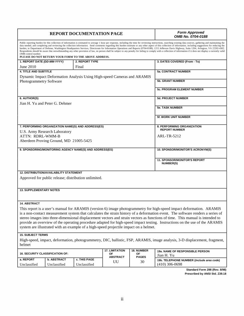
This report is a user’s manual for ARAMIS (version 6) image photogrammetry for high-speed impact deformation. ARAMIS is a non-contact measurement system that calculates the strain history of a deformation event. The software renders a series of stereo images into three-dimensional displacement vectors and strain vectors as functions of time. This manual is intended to provide an overview of the operating procedure adapted for high-speed impact testing. Instructions on the use of the ARAMIS system are illustrated with an example of a high-speed projectile impact on a helmet.
Figure 1. Two Phantom high-speed cameras for generating stereo images. .................................. 2
Figure 2. Calibration images taken in at the initial position of the calibration panel. ................... 3
Figure 3. Calibration images where the calibration panel was moved closer to the cameras at a distance no less than the expected deformation displacement of the target. ...................... 4
Figure 4. Calibration images where the calibration panel was moved away from the cameras. ..................................................................................................................................... 4
Figure 5. Calibration images where the calibration panel was moved back to its initial position, but with a tilt of 40° away from the line of sight. ...................................................... 5
Figure 6. Calibration image where the calibration panel was rotated 180° about its plane normal axis. ............................................................................................................................... 5
Figure 7. Calibration images where the calibration panel was moved back to its initial position but with its plane normal axis parallel to the left camera, showing an image taken for each 90° rotation. ....................................................................................................... 6
Figure 8. Calibration images where the calibration panel was moved back to its initial position but with its plane normal axis parallel to the left camera, showing images taken by the right camera with the panel facing it. ............................................................................. 6
Figure 12. Calibration result display. ........................................................................................... 10
Figure 13. Rejected calibration images: a) dots are too small, b) some dots are not processed, and c) dots are not recognized. ............................................................................. 11
Figure 14. Ideal apparent dot size: ~5×5 pixels (each square is a pixel)...................................... 12
Figure 19. Starting points for deformation analysis. .................................................................... 16
Figure 20. Computed net displacement on the helmet, 1.82 ms after impact: a) Facet size = 15, facet step = 13 and b) facet size =15, facet step = 11. ....................................................... 18
Figure 21. Computed net displacement on the helmet, 1.82 ms after impact: a) Facet size = 11, facet step = 9 and b) facet size = 9, facet step =7. ............................................................. 19
Figure 22. The noise filter menu . ................................................................................................ 20
v
Acknowledgments
We thank Dr. Shawn Walsh of RDRL-WMM-D for providing us the helmet. We thank Mr. Tim Schmidt of Trilion Quality Systems for training us on using the ARAMIS system.
vi
INTENTIONALLY LEFT BLANK.
1
1. Introduction
Photogrammetry is a technique that uses photographic images to determine the geometric properties of an object. The technique involves digitizing an imaged pattern on an object before and after a deformation has occurred. ARAMIS (GOM mbH, Braunschweig, Germany) is a commercial software package for three-dimensional (3-D) image photogrammetry. The software is an optical 3-D deformation measuring system that translates the movements of pixels in a series of stereo photographs into displacement vectors. By combining high-speed stereo photography and photogrammetry, one can obtain a detail history of a target that undergoes fast rate of deformation.
This report is a user’s manual for ARAMIS (version 6) image photogrammetry for high-speed impact deformation. Instructions on the use of the ARAMIS system are illustrated with an example of a high-speed projectile impact on a helmet.
2. Hardware
2.1 Fragment Simulating Projectile (FSP) Launching Apparatus
For our demonstration, we used a 0.22-caliber FSP launching apparatus to simulate the effects of high-speed fragment striking a helmet. The standard operating procedure and the setup for the FSP launch apparatus are detailed in another report1
2.2 High-speed Cameras
.
ARAMIS can accept TIFF images from any calibrated charge-coupled device (CCD) camera. In our demonstration, we used two Phantom high-speed cameras (model v7, Vision Research, Wayne, NJ) to generate stereo image pairs of the impact area. The lines-of-sight of the cameras were angled at no more than 25° with respect to each other (figure 1). The angle setting does not need to be exact; however, it is preferred that the lines-of-sight of the cameras are co-planar and the focal plane of the two cameras is the same.
1 Yu, J.; Dehmer, P.; Sands, J. The Current Capabilities on Dynamic Impact Testing; ARL-TR-4496; U.S. Army Research
Laboratory: Aberdeen Proving Ground, MD, July 2008.
2
Figure 1. Two Phantom high-speed cameras for generating stereo images.
2.3 Hardware Settings for the Helmet Impact Example
We used a 250- by 200-mm calibration panel. The focal length of the lens was set to 28 mm and the f-stop was set at f/8. The line-of-sight was 35° with respect to the path of the projectile and the cameras were ~20° apart. The distance between the cameras and the impact zone was ~1 m. The resolution of the images was set to 304 x 224 pixels, the exposure time to 20 ms, and the inter-frame time to 44 ms. A total of 300 pairs of sequential images were selected for photogrammetric analysis. All images were saved in TIFF format and placed under two file directories: “left” and “right” for the left and right camera images, respectively. The files were named sequentially, from “1.tif” to “500.tif” for each series.
3. Image Calibration for ARAMIS
3.1 Calibration Setup
For image calibration, we set the resolution of the cameras to their maximum value (800×600 pixels for the Phantom v7). The calibration process involves taking a series of images on a calibration panel. There are several panel sizes from which to choose. The ideal panel size is the one that occupies the field-of-view of the cameras fully. If the panel size is smaller than the field-of-view, the parameters need to be adjusted during the calibration process (see section 3.2).
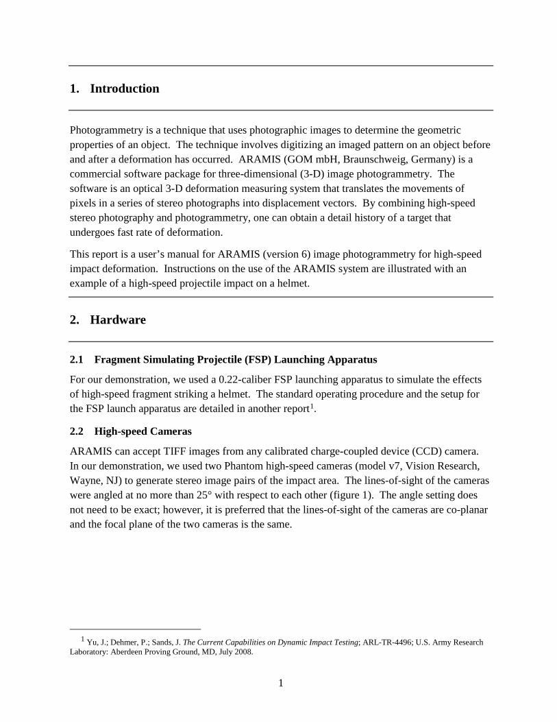
In the first step of the calibration process, the calibration panel was placed near the proposed impact location. Then, the lines-of-sight for the cameras were focused and centered on the calibration panel (figure 2a). The crosshairs indicate the aiming point of the cameras. The
3
cameras and lenses were locked in this position until the end of the entire impact experiment. Any camera or lens movement during the experiment would cause error in the displacement and strain calculations.
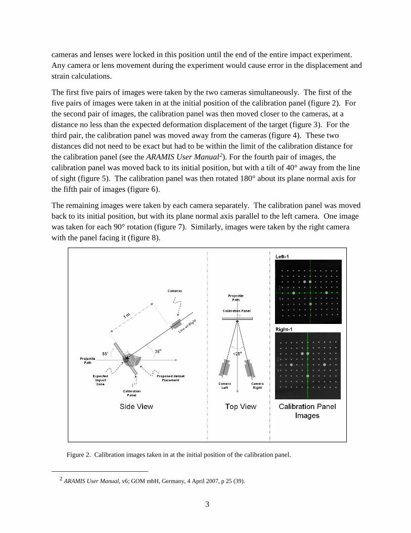
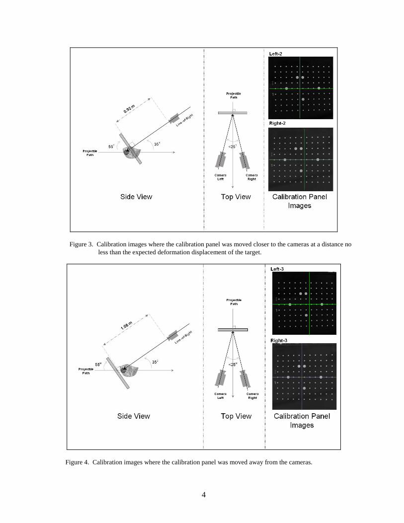
The first five pairs of images were taken by the two cameras simultaneously. The first of the five pairs of images were taken in at the initial position of the calibration panel (figure 2). For the second pair of images, the calibration panel was then moved closer to the cameras, at a distance no less than the expected deformation displacement of the target (figure 3). For the third pair, the calibration panel was moved away from the cameras (figure 4). These two distances did not need to be exact but had to be within the limit of the calibration distance for the calibration panel (see the ARAMIS User Manual2
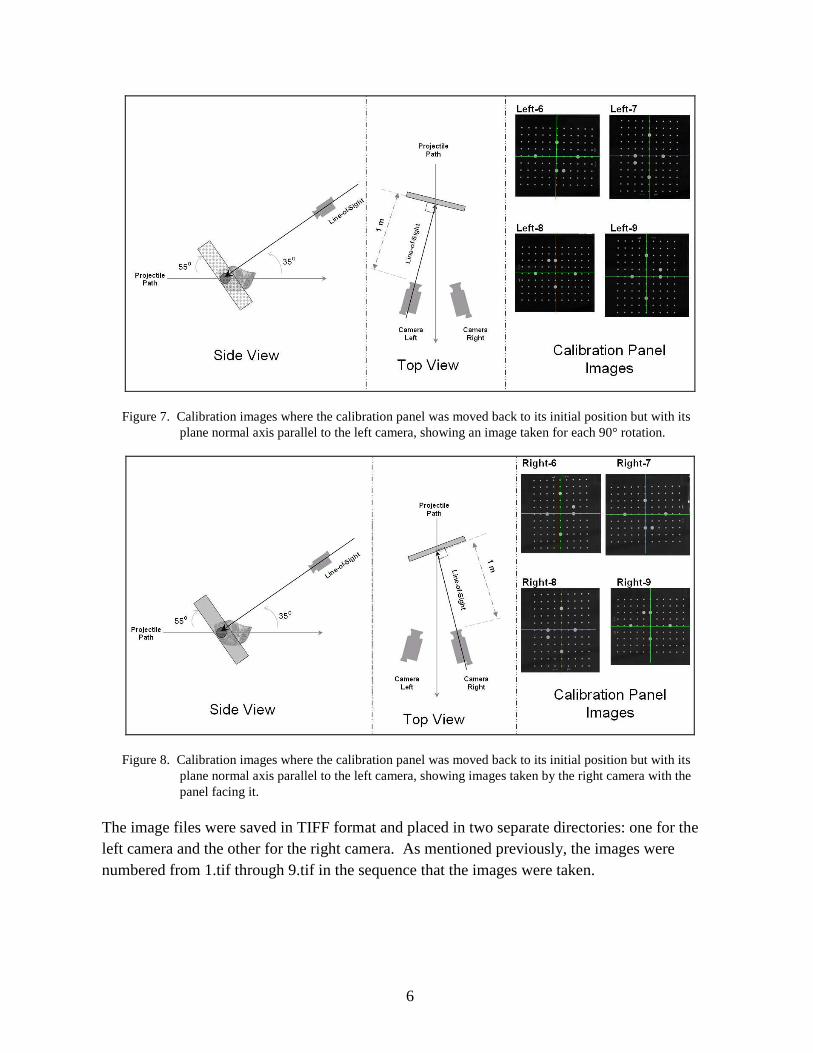
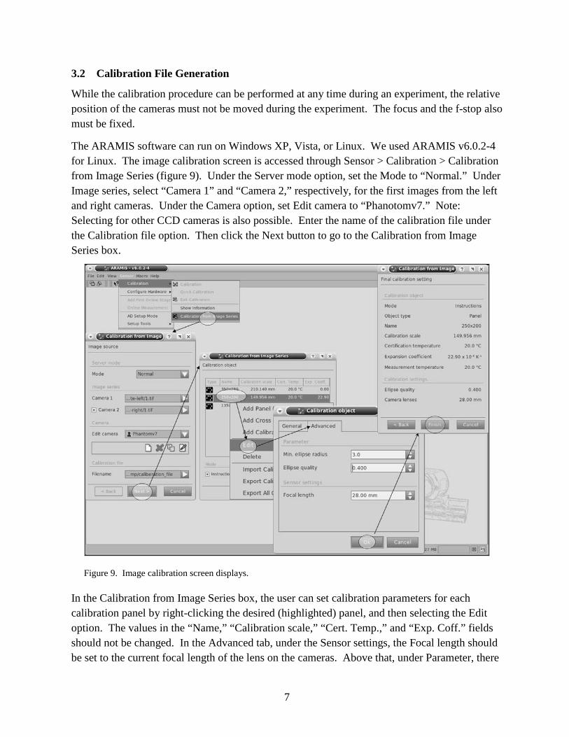
The remaining images were taken by each camera separately. The calibration panel was moved back to its initial position, but with its plane normal axis parallel to the left camera. One image was taken for each 90° rotation (figure 7). Similarly, images were taken by the right camera with the panel facing it (figure 8).
). For the fourth pair of images, the calibration panel was moved back to its initial position, but with a tilt of 40° away from the line of sight (figure 5). The calibration panel was then rotated 180° about its plane normal axis for the fifth pair of images (figure 6).
Figure 2. Calibration images taken in at the initial position of the calibration panel.
2 ARAMIS User Manual, v6; GOM mbH, Germany, 4 April 2007, p 25 (39).
4
Figure 3. Calibration images where the calibration panel was moved closer to the cameras at a distance no less than the expected deformation displacement of the target.
Figure 4. Calibration images where the calibration panel was moved away from the cameras.
5
Figure 5. Calibration images where the calibration panel was moved back to its initial position, but with a tilt of 40° away from the line of sight.
Figure 6. Calibration image where the calibration panel was rotated 180° about its plane normal axis.
6
Figure 7. Calibration images where the calibration panel was moved back to its initial position but with its plane normal axis parallel to the left camera, showing an image taken for each 90° rotation.
Figure 8. Calibration images where the calibration panel was moved back to its initial position but with its plane normal axis parallel to the left camera, showing images taken by the right camera with the panel facing it.
The image files were saved in TIFF format and placed in two separate directories: one for the left camera and the other for the right camera. As mentioned previously, the images were numbered from 1.tif through 9.tif in the sequence that the images were taken.
7
3.2 Calibration File Generation
While the calibration procedure can be performed at any time during an experiment, the relative position of the cameras must not be moved during the experiment. The focus and the f-stop also must be fixed.
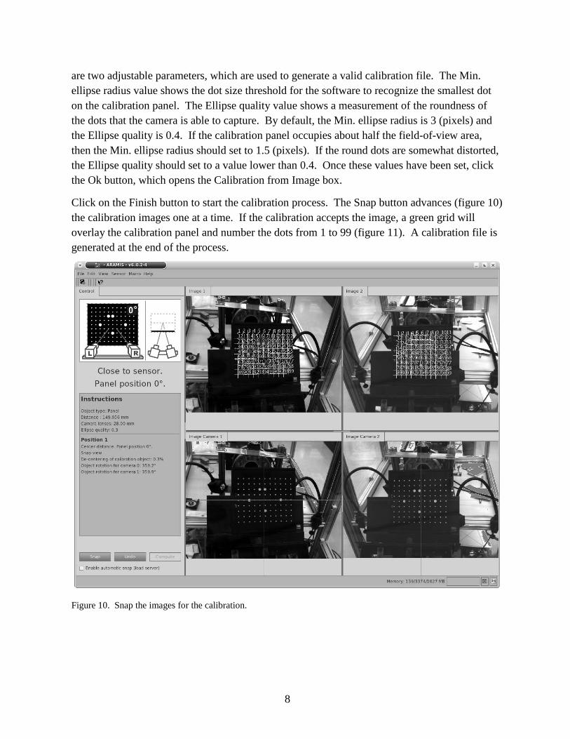
The ARAMIS software can run on Windows XP, Vista, or Linux. We used ARAMIS v6.0.2-4 for Linux. The image calibration screen is accessed through Sensor > Calibration > Calibration from Image Series (figure 9). Under the Server mode option, set the Mode to “Normal.” Under Image series, select “Camera 1” and “Camera 2,” respectively, for the first images from the left and right cameras. Under the Camera option, set Edit camera to “Phanotomv7.” Note: Selecting for other CCD cameras is also possible. Enter the name of the calibration file under the Calibration file option. Then click the Next button to go to the Calibration from Image Series box.
Figure 9. Image calibration screen displays.
In the Calibration from Image Series box, the user can set calibration parameters for each calibration panel by right-clicking the desired (highlighted) panel, and then selecting the Edit option. The values in the “Name,” “Calibration scale,” “Cert. Temp.,” and “Exp. Coff.” fields should not be changed. In the Advanced tab, under the Sensor settings, the Focal length should be set to the current focal length of the lens on the cameras. Above that, under Parameter, there
8
are two adjustable parameters, which are used to generate a valid calibration file. The Min. ellipse radius value shows the dot size threshold for the software to recognize the smallest dot on the calibration panel. The Ellipse quality value shows a measurement of the roundness of the dots that the camera is able to capture. By default, the Min. ellipse radius is 3 (pixels) and the Ellipse quality is 0.4. If the calibration panel occupies about half the field-of-view area, then the Min. ellipse radius should set to 1.5 (pixels). If the round dots are somewhat distorted, the Ellipse quality should set to a value lower than 0.4. Once these values have been set, click the Ok button, which opens the Calibration from Image box.
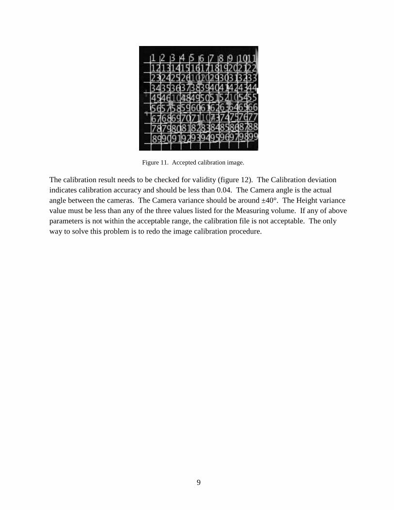
Click on the Finish button to start the calibration process. The Snap button advances (figure 10) the calibration images one at a time. If the calibration accepts the image, a green grid will overlay the calibration panel and number the dots from 1 to 99 (figure 11). A calibration file is generated at the end of the process.
Figure 10. Snap the images for the calibration.
9
Figure 11. Accepted calibration image.
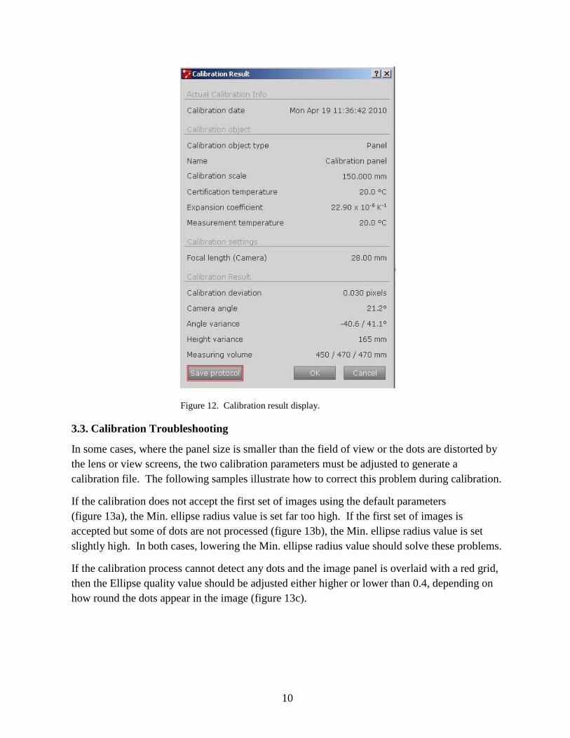
The calibration result needs to be checked for validity (figure 12). The Calibration deviation indicates calibration accuracy and should be less than 0.04. The Camera angle is the actual angle between the cameras. The Camera variance should be around ±40°. The Height variance value must be less than any of the three values listed for the Measuring volume. If any of above parameters is not within the acceptable range, the calibration file is not acceptable. The only way to solve this problem is to redo the image calibration procedure.
10
Figure 12. Calibration result display.
3.3. Calibration Troubleshooting
In some cases, where the panel size is smaller than the field of view or the dots are distorted by the lens or view screens, the two calibration parameters must be adjusted to generate a calibration file. The following samples illustrate how to correct this problem during calibration.
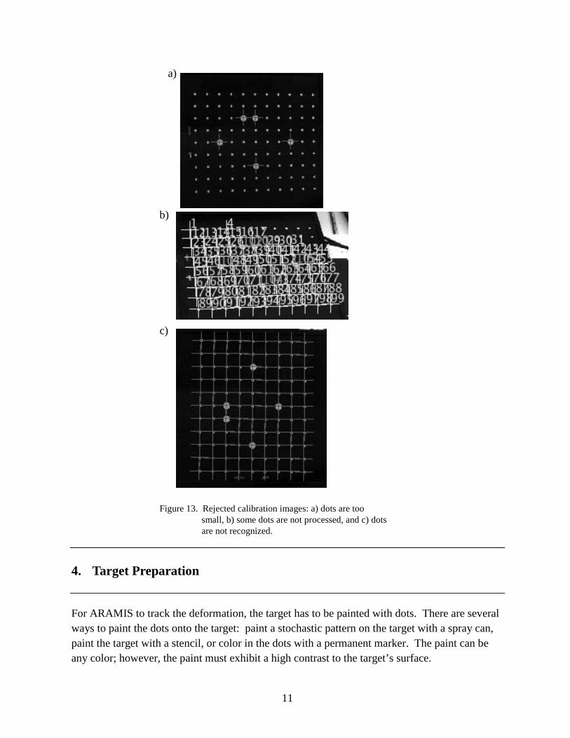
If the calibration does not accept the first set of images using the default parameters (figure 13a), the Min. ellipse radius value is set far too high. If the first set of images is accepted but some of dots are not processed (figure 13b), the Min. ellipse radius value is set slightly high. In both cases, lowering the Min. ellipse radius value should solve these problems.
If the calibration process cannot detect any dots and the image panel is overlaid with a red grid, then the Ellipse quality value should be adjusted either higher or lower than 0.4, depending on how round the dots appear in the image (figure 13c).
11
a)
b)
c)
Figure 13. Rejected calibration images: a) dots are too small, b) some dots are not processed, and c) dots are not recognized.
4. Target Preparation
For ARAMIS to track the deformation, the target has to be painted with dots. There are several ways to paint the dots onto the target: paint a stochastic pattern on the target with a spray can, paint the target with a stencil, or color in the dots with a permanent marker. The paint can be any color; however, the paint must exhibit a high contrast to the target’s surface.
12
The ideal apparent dot size is ~5×5 pixels as it is rendered in an image file. The apparent dot size depends on the focal length of the lens; the distance between the camera and the target; and the resolution setting of the image. The best way to determine the required dot size is to take an image of painted dots of various sizes; the desired dot size is the one that appears to be ~5×5 pixels (figure 14).
Figure 14. Ideal apparent dot size: ~5×5 pixels (each square is a pixel).
For the helmet used in the demonstration, we painted on the dots with a permanent marker. The dots were ~4.5 mm in diameter and were separated by an average of 2.5 mm space between the dots (figure 15).
Figure 15. Painted helmet.
13
5. Deformation Analysis
5.1 Computation Setup
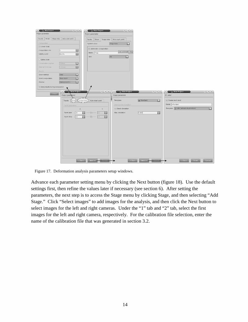
To start the deformation analysis, under File, select “New Project” and enter a name for the project (figure 16). After naming the project and selecting 3D analysis, the project parameter screens opens (figure 17). The details on selecting appropriate parameters are summarized in sections 5.2 and 6 of this report. The default parameters are used here.
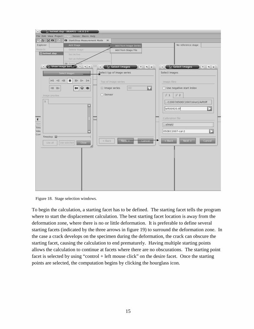
Advance each parameter setting menu by clicking the Next button (figure 18). Use the default settings first, then refine the values later if necessary (see section 6). After setting the parameters, the next step is to access the Stage menu by clicking Stage, and then selecting “Add Stage.” Click “Select images” to add images for the analysis, and then click the Next button to select images for the left and right cameras. Under the “1” tab and “2” tab, select the first images for the left and right camera, respectively. For the calibration file selection, enter the name of the calibration file that was generated in section 3.2.
15
Figure 18. Stage selection windows.
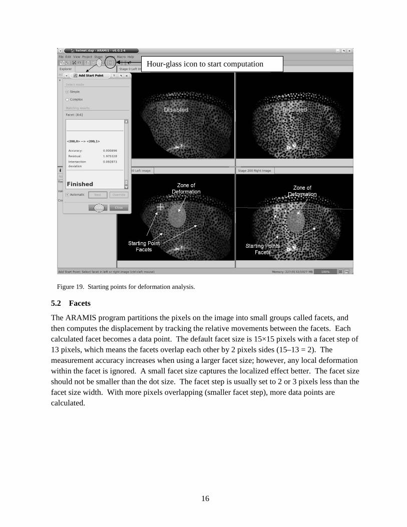
To begin the calculation, a starting facet has to be defined. The starting facet tells the program where to start the displacement calculation. The best starting facet location is away from the deformation zone, where there is no or little deformation. It is preferable to define several starting facets (indicated by the three arrows in figure 19) to surround the deformation zone. In the case a crack develops on the specimen during the deformation, the crack can obscure the starting facet, causing the calculation to end prematurely. Having multiple starting points allows the calculation to continue at facets where there are no obscurations. The starting point facet is selected by using “control + left mouse click” on the desire facet. Once the starting points are selected, the computation begins by clicking the hourglass icon.
16
Figure 19. Starting points for deformation analysis.
5.2 Facets
The ARAMIS program partitions the pixels on the image into small groups called facets, and then computes the displacement by tracking the relative movements between the facets. Each calculated facet becomes a data point. The default facet size is 15×15 pixels with a facet step of 13 pixels, which means the facets overlap each other by 2 pixels sides (15–13 = 2). The measurement accuracy increases when using a larger facet size; however, any local deformation within the facet is ignored. A small facet size captures the localized effect better. The facet size should not be smaller than the dot size. The facet step is usually set to 2 or 3 pixels less than the facet size width. With more pixels overlapping (smaller facet step), more data points are calculated.
Hour-glass icon to start computation
17
5.3 Strain Calculation
ARAMIS has a built-in algorithm to compute the strain field. However, the strain calculation should be used with caution, because the algorithm assumes the deformed body is continuous. Only the in-plane strains in the 11 and 22 directions are computed from the displacement field. The strain in the 33 (out-of-plane) direction is calculated by plane stress or plane strain models. Incompressibility of the solid body is assumed.
There are two ways to compute the strain from the data points: linear strain computation and spline strain computation. The linear strain computation uses displacement data points (facets points) to calculate the strain, whereas the spline strain computation interpolates the displacement data points to create additional points first and then uses both the interpolated and original data points to calculate the strain.
The default linear strain computation size is three, which means a total of nine neighboring facet points, including the center facet, are used to compute the strain at the center facet. A large computation size reduces the noise, but it also may reduce the total number of strain computation points. A validity quote of 100% means 100% of the neighboring facets points must be present in order to compute the strain. This value is usually not set to 100%. Instead, it is set to 55% in order to compute the strain near the edges or cracks on the target.
The spline strain computation is able to compute the strain in a location where there is a small radius of curvature. The spline strain can calculate the strain on the surface or in the middle of the target. There are also two ways to present the computed strain results: the total strain method and the step-by-step method. The first method uses the first stage as the reference stage, whereas the latter method always uses the previous to current stages. To compute the stress on the target, the material properties, such as the Young’s modulus, are required. The plane stress model is appropriate for thin materials, whereas the plane strain model is suitable for thick material.
6. Other Parameter Settings
6.1 Stage Parameter Settings
If the picture files contain metadata about the frame rate, the inter-stage time is automatically computed. Otherwise, the stage number represents the inter-stage time. The computation template option can be set to “High Accuracy” for all calculations (figure 17). The intersection deviation value can be set to 0.3 pixels or higher, which is a criterion to accept or reject a computed facet point depending on the deviation between measurements from the two cameras. Setting a value higher than 0.3, however, can lead to a result value error.
18
6.2 Facet Size and Facet Step
The maximum displacements on the impact zone were first computed with the default settings, and then with other computational settings for various facet sizes and step sizes. Using the default settings, the displacement profile (figure 20a) showed a sharp deformation at the apex of the impact zone. On the helmet, the apex of the impact of zone was actually quite blunt. Using a smaller facet step (11 pixels), the computed displacement profile (figure 20b) showed a more blunted feature at the apex than the default computation. Using a facet size of 11 and a facet step of 9, more features on the impact zone were captured (figure 21a), especially near the edge of the impact zone. If the facet size was decreased further to 9 pixels, missing facet points started to appear (figure 20b). The facet size was too small to track the movement of the dots. In general, the facet step can be set as small as 3. In the helmet case, setting the facet size and the facet step as 11 and 9, respectively, yielded a more accurate result than other settings.
a) Facet size = 15, facet step = 13
b) Facet size =15, facet step = 11
Figure 20. Computed net displacement on the helmet, 1.82 ms after impact: a) Facet size = 15, facet step = 13 and b) facet size =15, facet step = 11.
19
a) Facet size = 11, facet step = 9
b) Facet size = 9, facet step = 7
Figure 21. Computed net displacement on the helmet, 1.82 ms after impact: a) Facet size = 11, facet step = 9 and b) facet size = 9, facet step =7.
6.3 Noise Filter
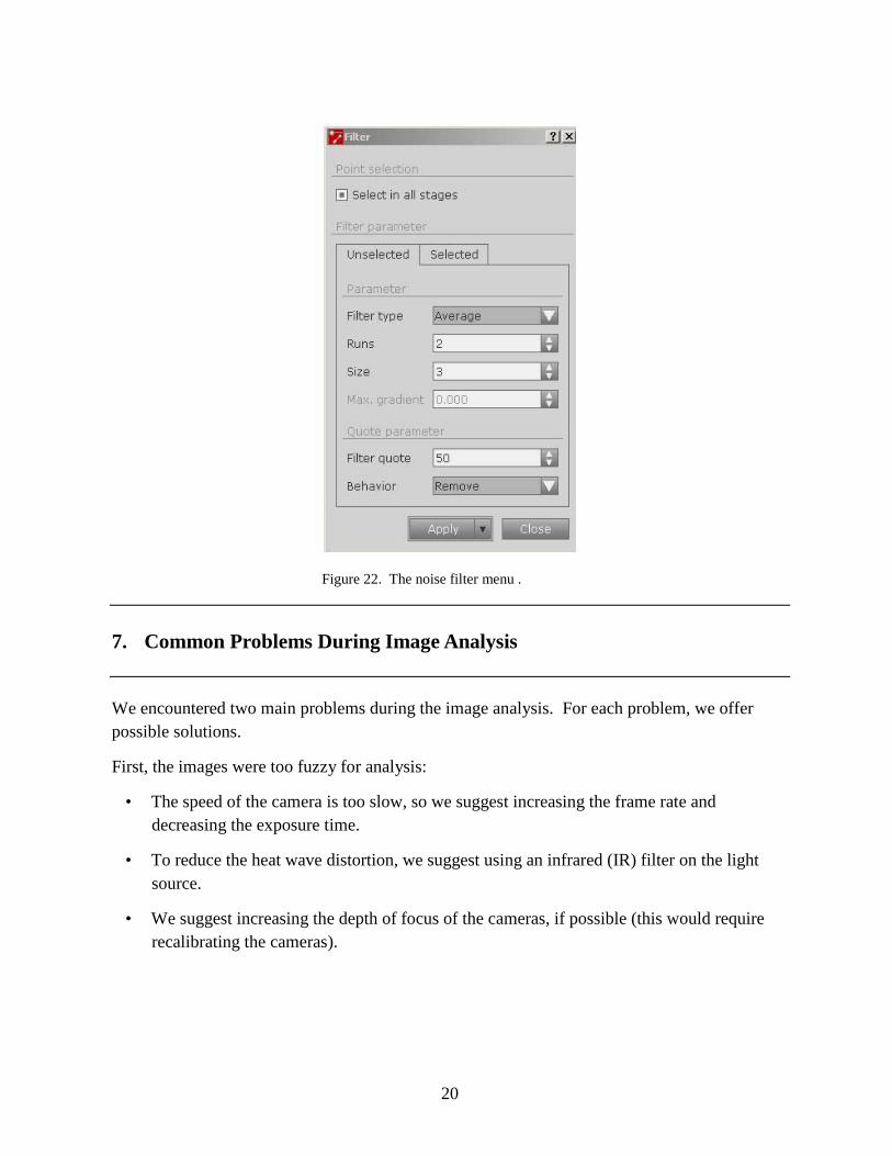
To reduce noise, the filtering option can be accessed by selecting the Results menu and then Filter. Usually, an average run of 2 and a size of 3 are sufficient to remove the noise (figure 22). Any higher settings can induce errors in the actual measurement.
20
Figure 22. The noise filter menu .
7. Common Problems During Image Analysis
We encountered two main problems during the image analysis. For each problem, we offer possible solutions.
First, the images were too fuzzy for analysis:
• The speed of the camera is too slow, so we suggest increasing the frame rate and decreasing the exposure time.
• To reduce the heat wave distortion, we suggest using an infrared (IR) filter on the light source.
• We suggest increasing the depth of focus of the cameras, if possible (this would require recalibrating the cameras).
21
Second, there were missing facets:
• We suggest increasing the facet size.
• There was not enough contrast, we suggest painting more dots.
• The illumination is dark or too bright; we suggest increasing or decreasing the light intensity.
• There were spots of glare on the impact site. We suggest painting the impact site with a flat black paint, if possible, and using a flat yellow paint as contrast. Also, using a light diffuser or a diffused light source would help.
• The paint did not adhere to the surface of the target. We recommend using Sharpie® ink.
• Cracks and chips developed on the target during the impact. We recommend using the Interpolate function; however, it may give an inaccurate result.
22
No. of Copies Organization 1 ADMNSTR ELEC DEFNS TECHL INFO CTR ATTN DTIC OCP 8725 JOHN J KINGMAN RD STE 0944 FT BELVOIR VA 22060-6218 3 US ARMY RSRCH LAB ATTN IMNE ALC HRR MAIL & RECORDS MGMT ATTN RDRL CIM L TECHL LIB ATTN RDRL CIM P TECHL PUB ADELPHI MD 20783-1197 1 US ARMY RSRCH LAB ATTN RDRL CIM G T LANDFRIED BLDG 4600 ABERDEEN PROVING GROUND MD 21005-5066 5 US ARMY RSRCH LAB ATTN RDRL WMM B M VANLANDINGHAM J YU ATTN RDRL WMM D S WALSH L VARGAS-GONZALEZ ATTN RDRL WMM E P DEHMER BLDG 4600 ABERDEEN PROVING GROUND MD 21005-5066
No. of Copies Organization 1 US ARMY RSRCH LAB ATTN RDRL SLB D J GURGANUS BLDG 1068 ABERDEEN PROVING GROUND MD 21005-5066 1 US ARMY RSRCH LAB ATTN RDRL SLB D D HISLEY BLDG 238 ABERDEEN PROVING GROUND MD 21005-5066 2 US ARMY RSRCH LAB ATTN RDRL WMP B