Dynamic Information Acquisition and Home Bias in Portfolios (Preliminary and Incomplete) Rosen Valchev * Boston College March 2017 Abstract While international portfolios are still heavily biased towards home assets, the home bias has exhibited a clear downward trend in the last few decades. Interestingly, the underlying rise in foreign investment has been primarily directed to just a handful of OECD countries, and has not given rise to an across the board increase in all foreign investments. To understand the evolution of the home bias, this paper develops a dynamic model of information acquisition and portfolio choice. The dynamic framework introduces two new endogenous forces due to the fact that asset payoffs depend on the future asset prices and hence on the future information sets. First, there is a measure of endogenous unlearnable uncertainty in asset payoffs which generates decreasing returns to information when agents are sufficiently well informed about an asset, and hence gives a reason to diversify information and portfolios. In addition, the dynamic framework introduces a strategic complementarity in learning, due to the “beauty contest” of dynamic asset markets, which is absent in the benchmark static model where learning is purely a strategic substitute. As a result of both of these new endogenous forces, the model can explain the high overall level of the home bias, its decline over time and the fact that the rise in foreign investment has been coordinated on just a handful of destination countries. Moreover, the model predicts that the home bias de- cline is linked to the fall in information costs, and I find direct evidence of this in the data. JEL Codes: F3, G11, G15, D8, D83 Keywords: Home Bias, Information Choice, Portfolio Choice, Dynamics * I am deeply grateful to Craig Burnside and Cosmin Ilut for numerous thoughtful discussions. I am also thankful to Francesco Bianchi, Ryan Chahrour, Yuriy Gorodnichenko, Tarek Hassan, Nir Jaimovich, Julien Hugonnier, Alisdair McKay, Jianjun Miao, Jaromir Nosal, Pietro Peretto, Adriano Rampini, Steven Riddiough, Oleg Rytchkov, Michael Siemer, Tong Zhou, and seminar participants at Boston College, Chicago Booth International Finance Meeting, Duke, ESEM, Green Line Macro Meetings, Midwest Finance Meetings, Midwest Macro Meetings, and Northern Finance Association. All remaining mistakes are mine. Contact Information – Boston College, Department of Economics; e-mail: [email protected]
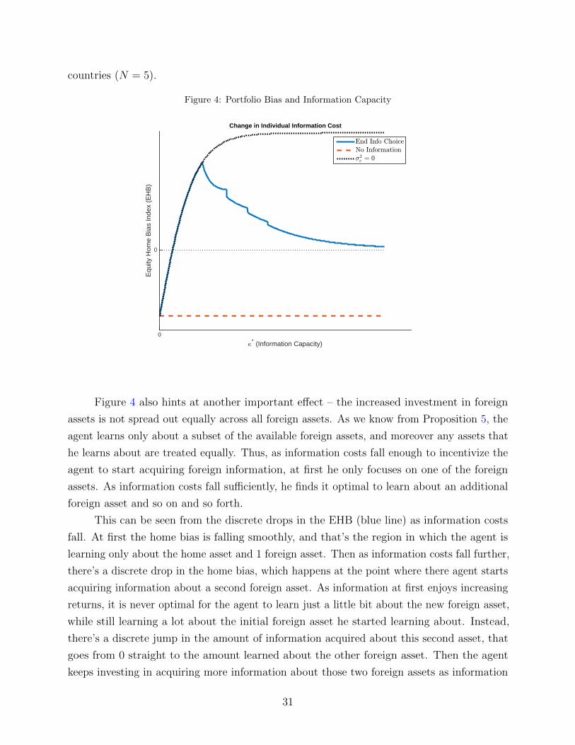
Transcript
Dynamic Information Acquisition and Home
Bias in Portfolios
(Preliminary and Incomplete)
Rosen Valchev∗
Boston College
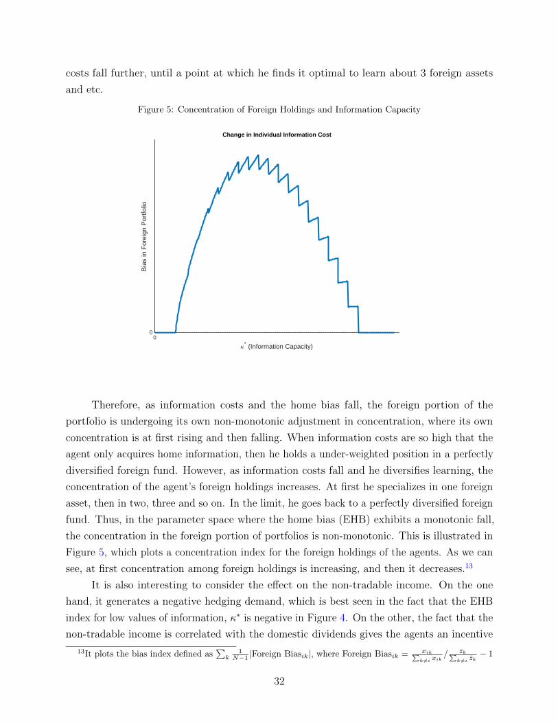
March 2017
Abstract
While international portfolios are still heavily biased towards home assets, the home
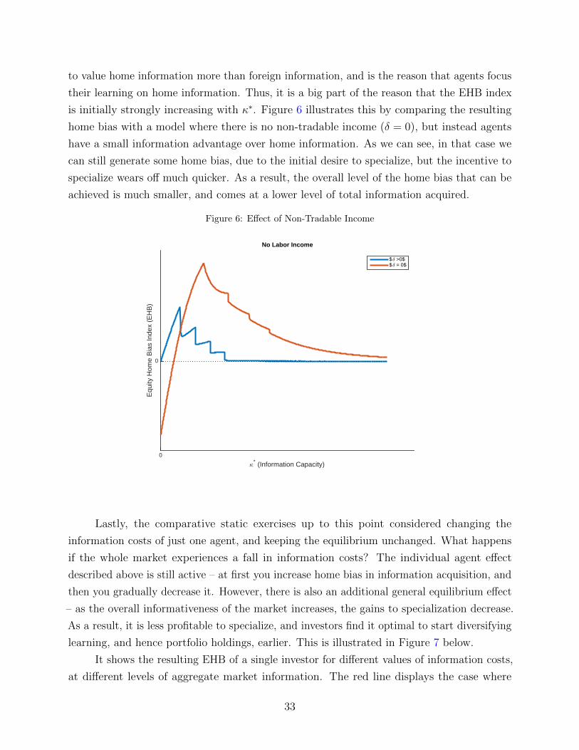
bias has exhibited a clear downward trend in the last few decades. Interestingly, the
underlying rise in foreign investment has been primarily directed to just a handful of
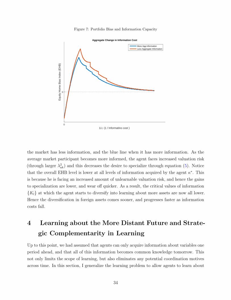
OECD countries, and has not given rise to an across the board increase in all foreign
investments. To understand the evolution of the home bias, this paper develops a
dynamic model of information acquisition and portfolio choice. The dynamic framework
introduces two new endogenous forces due to the fact that asset payoffs depend on the
future asset prices and hence on the future information sets. First, there is a measure
of endogenous unlearnable uncertainty in asset payoffs which generates decreasing
returns to information when agents are sufficiently well informed about an asset, and
hence gives a reason to diversify information and portfolios. In addition, the dynamic
framework introduces a strategic complementarity in learning, due to the “beauty
contest” of dynamic asset markets, which is absent in the benchmark static model where
learning is purely a strategic substitute. As a result of both of these new endogenous
forces, the model can explain the high overall level of the home bias, its decline over
time and the fact that the rise in foreign investment has been coordinated on just a
handful of destination countries. Moreover, the model predicts that the home bias de-
cline is linked to the fall in information costs, and I find direct evidence of this in the data.
JEL Codes: F3, G11, G15, D8, D83
Keywords: Home Bias, Information Choice, Portfolio Choice, Dynamics
∗I am deeply grateful to Craig Burnside and Cosmin Ilut for numerous thoughtful discussions. I amalso thankful to Francesco Bianchi, Ryan Chahrour, Yuriy Gorodnichenko, Tarek Hassan, Nir Jaimovich,Julien Hugonnier, Alisdair McKay, Jianjun Miao, Jaromir Nosal, Pietro Peretto, Adriano Rampini, StevenRiddiough, Oleg Rytchkov, Michael Siemer, Tong Zhou, and seminar participants at Boston College, ChicagoBooth International Finance Meeting, Duke, ESEM, Green Line Macro Meetings, Midwest Finance Meetings,Midwest Macro Meetings, and Northern Finance Association. All remaining mistakes are mine. ContactInformation – Boston College, Department of Economics; e-mail: [email protected]
1 Introduction
Empirical evidence indicates that investors fail to take sufficient advantage of international
diversification opportunities, and heavily overweight domestic equities in their portfolios.1
This phenomenon is commonly referred to as the “home equity bias”, and is a long standing
issue in international finance that is especially puzzling since it has persisted decades after the
liberalization of international capital flows in the 80s. It has given rise to a large and active
literature, and a number of potential explanations have been proposed, such as endogenous
information asymmetry (Van Nieuwerburgh and Veldkamp (2009)), hedging of non-tradable
labor income (Coeurdacier and Gourinchas (2011), Heathcote and Perri (2007)), behavioral
models (e.g. Huberman (2001)) and others.
However, the primary focus of the existing literature has been on rationalizing the
overall level of the home bias, while its more recent trend downward has received considerably
less attention. And although the home bias is still a significant puzzle, it has declined
markedly over the last two decades – the average level of foreign asset holdings around the
world have increased from being just 10% of the benchmark CAPM prediction in 1995 up
to 35% of CAPM in 2015. However, this rise in foreign investment has not been equally
distributed across the world, but has rather been primarily directed to just a handful of
OECD countries. Thus, while investors are holding more foreign equity than before, their
foreign holdings themselves tend to be highly concentrated. This evolution of the home bias
over the last few decades is a salient feature of the data and understanding it could shed new
light on the puzzle as a whole. Nevertheless, existing models are static and do not speak
directly to its movements over time.
This paper develops a dynamic model of endogenous information acquisition that can
address both the high overall level of the home bias, and its decline over time. It extends
the benchmark, static model of Van Nieuwerburgh and Veldkamp (2009) by introducing
overlapping generation of agents and infinitely lived assets. Similar to that model, there is
a feedback between information and portfolio choice that generates increasing returns to
information, and agents find it optimal to specialize their information acquisition in domestic
assets, which leads to strong information asymmetry and home bias in equilibrium. However,
in my model, asset markets are open every period, and thus asset payoffs depend not only
on dividends but also on the future equilibrium market price. These prices are determined
by the information available to future market participants, which introduces a measure of
endogenous unlearnable uncertainty. This weakens the feedback effect between information
and portfolio choice, and helps generate decreasing returns to information when agents are
1See for example French and Poterba (1991), Tesar and Werner (1998), Ahearne et al. (2004)
1
relatively well informed about a given asset.2
In addition, the dynamic nature of the asset markets in this economy introduces a
“beauty contest” motive, where agents would like to forecast future market beliefs, as those
determine the future price at which they can resell the asset. As a result, information is no
longer a pure strategic substitute. In a static model, agents want to learn about things that
the market does not know because this allows them to exploit any mis-pricing – intuitively,
they are trying to identify “under-valued” assets. However, in the dynamic model agents
have somewhat different incentives – they want to identify assets that are i) mis-priced by
the market and ii) are likely to be properly priced in the future. If the market does not
eventually correct the mis-pricing identified by an investor’s private information, then the
future price would not adjust appropriately and hence the investor would not profit from
identifying this mis-pricing. Intuitively, in the dynamic model it makes sense to invest in
under-valued assets only to the extent to which you expect future market beliefs to agree
with you that the asset was undervalued in the first place. As a result, this gives rise to a
strategic complementarity in learning that is absent from the static model, where learning is
purely a strategic substitute. Combined with the endogenous unlearnable uncertainty, these
two mechanisms allow the dynamic model to obtain a high level of home bias, a profile that
is declining over time (as information costs fall), and the observation that the increase in
foreign investment is concentrated in just a handful of advanced markets (where the average
investor is well informed).
In the model, there are N countries, each of which is populated by a continuum of
overlapping generations that live for two periods.3 In each country there is a Lucas tree with a
stochastic dividend, a portion of which is traded internationally, and the rest is a non-tradable
endowment of the domestic agents. The payoff of the Lucas tree is driven by a persistent
process that is specific to each country. The Young agents of each generation are born with
some initial wealth that they invest in the N risky assets and a riskless international bond.
The Old agents sell all of their assets to the new generation of Young agents, consume the
proceeds plus their non-tradable endowment, and exit.
When making their portfolio choice, agents see the whole history of state variables and
can purchase noisy signals about the realization of future economic fundamentals. Information
is valuable because it reduces the uncertainty about future consumption, which depends on
portfolio returns and the non-tradable endowment. Moreover, information is non-rival, and
hence a unit of information about the home fundamental factor can be used equally well
2 In a different framework, Veldkamp (2011), shows that exogenously introducing unlearnable risk canlead to interior solutions in the static model. In the dynamic model studied here, however, unlearnableuncertainty is not imposed exogenously but arises as a consequence of equilibrium forces.
3Similar to the setup in Bacchetta and van Wincoop (2006).
2
to learn about the future dividend of the home tradable asset and the future non-tradable
income. Thus, due to its dual use, domestic information has a relatively higher value, and
as a result agents tilt their costly information acquisition towards it, leading to information
asymmetry and home biased portfolios.4
In addition, there is a feedback loop between information acquisition and portfolio choice.
Information decreases the uncertainty of an asset’s return, and as a result investors increase
their portfolio holdings of that asset. As the holdings of the asset increase, however, the next
unit of information about this asset is now more valuable to the agent, since information
is non-rival and hence more valuable when applied to a bigger trade. Thus, an initial tilt
towards home information leads to portfolio re-balancing that increases the relative value
of home information further, which in turn leads to another shift toward home information
and so on. This feedback loop is at the heart of the increasing returns to information that
obtain globally in the standard static framework, however in the dynamic model there is also
a countervailing equilibrium force.
Since returns depend on future market prices, and thus on future market beliefs, to
the extent to which information available today cannot fully span future market beliefs,
investors are exposed to some unlearnable uncertainty encoded in asset prices. This changes
the incentives to specialize. Rebalancing the portfolio towards home assets makes investors
increasingly exposed to the unlearnable valuation risk in future home asset prices, and thus
increases the non-diversifiable risk of the portfolio. This moderates the feedback between
information and portfolio choice, and as a result, increases in home information lead to smaller
adjustments in portfolios. This effect grows stronger as investors have learned more about a
specific asset, and unlearnable uncertainty becomes a larger share of its residual uncertainty.
In essence, information acquisition helps reduce an ever smaller proportion of the remaining
uncertainty, and the effect of the unlearnable valuation risk eventually comes to dominate,
and the increasing returns to information disappear. Thus, investors face increasing returns
to information about an asset when they have acquired relatively little information about
that asset, and face decreasing returns otherwise.
Consequently, information asymmetry and home bias have a non-monotonic relationship
with the ability to acquire information. When information is scarce, it is optimal to specialize
fully, and learn only about the domestic fundamental, while when information is abundant,
agents spread out learning across a variety of different factors. So as information costs fall, the
home bias is at first increasing, when information is still relatively scarce, and then decreases
4Non-diversifiable labor income plays a similar role in swaying information choice in Nieuwerburgh andVeldkamp (2006), who study the own company stock bias in a static framework. I extend the analysis to adynamic setting, and focus on the interaction between the resulting decreasing returns to information andnon-tradable income and its implications about the secular decline of the home bias.
3
as information becomes more abundant. As a result, the dynamic model can generate both a
high overall level of home bias, due to the incentives to specialize in domestic information
initially, and a gradual decline as information costs fall.
Note that in the model, information is generally a strategic substitute, as is also true in
the benchmark static model. Agents have incentives to try and learn information that the
rest of the market does not know, because they profit from exploiting the pricing mistakes of
the average market participant. Hence, in equilibrium agents try to hold information sets
that are different from those of the average market participant. Similarly, the incentive to
specialize is also a strategic substitute – agents are more likely to face increasing returns
to information about an asset if the market knows relatively little about it. Still, those
forces are not enough to generate increasing returns to information by themselves. While
agents want to be different, they realize that in making themselves so they incur increasing
exposure to unlearnable valuation risk. Thus, the recursive nature of the dynamic model
introduces an effect leading towards decreasing returns to information, even in frameworks
where information would otherwise have increasing returns. Lastly, in the dynamic model
information is not always a strategic substitute but becomes a strategic complement at higher
levels of information. As a result, once investors decide to diversify learning in foreign assets,
they tend to coordinate on markets where the average participant is better informed. This is
also true in the data, as most of the foreign investment underpinning the fall in the home
bias has been concentrated in just a few OECD markets.
Importantly, the share of unlearnable uncertainty in the dynamic model is an endogenous
quantity. As such, it changes as other market participants change their information acquisition
choices. This has a number of interesting implications, two of which I explore in more detail
in the paper. First, an increase in aggregate information increases the unlearnable uncertainty
faced by any given agent, because it makes future market beliefs more sensitive to future
news. As a result, the incentives to specialize in information acquisition, and thus home
bias itself, decrease for all agents. This is a general equilibrium effect that is distinct from
the fact that home bias tends to decrease as individual information increases. For example,
it implies that when informed foreign investors enter a new market, the home bias of the
domestic agents will decrease, as the share of unlearnable uncertainty increases, and thus,
the incentives to specialize in domestic information decrease. Second, because agents face
increasing returns to information when learning about a new asset, foreign assets are added
to the learning portfolio in a discrete fashion. As a result, the capital flows in the model can
exhibit fickleness and retrenchment.
The model makes a clear prediction that the home bias decline is linked with falling
information costs. This is intuitively appealing, because the sharp decline in the home bias
4
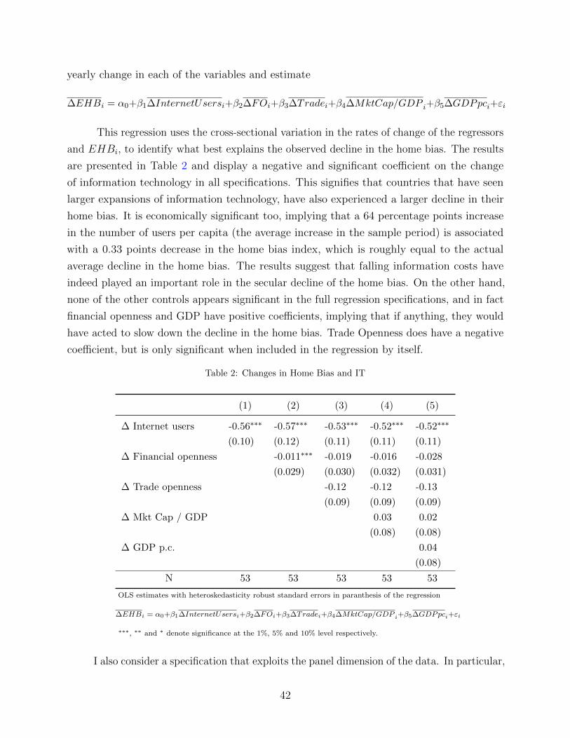
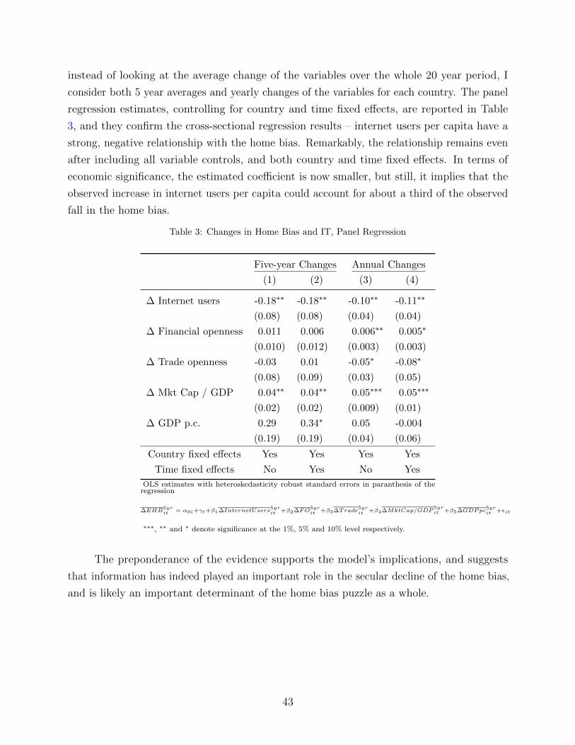
over the last two decades has coincided with the information technology (IT) boom. To test
this hypothesis rigorously, I examine the relationship between the growth of IT and the rate
of decline in the home bias for a broad sample of fifty-three countries. Consistent with the
model, I find a clear negative relationship, signifying that countries which have experienced a
larger expansion in IT exhibit stronger decline in the home bias. The relationship persists
after controlling for other potential covariates and country and time fixed effects, suggesting
that falling information costs indeed play an important role in the decline of the home bias.5
Lastly, while the model predicts that falling information costs are generally associated
with a fall in the home bias, this is not true for the concentration of the foreign portion
of the portfolio. This happens because the return to information is increasing at first, but
decreasing after a critical threshold of total information about an asset is reached. As a result,
once investors start diversifying learning into foreign assets, they do not do so equally across
all assets. Instead, they first specialize in just one foreign asset and start learning about
others, one by one, only as information costs fall even further. Thus, the concentration of
the foreign portion of portfolios has interesting dynamics as well, and the catchall home bias
measure does not necessarily tell the whole story. Moreover, the strategic complementarity
in learning ensures that investors around the world will choose to invest in the same handful
of advanced countries, where the markets are well informed. I show this is true in the data
as well, where for the average country, the great majority of the home bias decline has come
about as the result of changes in the holdings of equity in just a few OECD countries.
A closely related paper is Mondria and Wu (2010), who also study the decline in the
home bias using a modified version of the Van Nieuwerburgh and Veldkamp (2009) model.
However, their model is not fully dynamic, but is rather a repeated static game, which makes
the information acquisition problem quite similar to the standard static framework, and
inherits its global increasing returns to information and does not feature any complementarity
in learning across periods. The main innovation in their paper is to generalize the structure
of the private information signals, allowing the agents to learn about linear combinations of
the fundamentals. In that framework, they show that a transition from financial autarky to
frictionless international financial markets could lead to a fall in the home bias, however, their
model still implies that lower information costs lead to higher home bias. In contrast, my
model focuses on how multi-period assets and the resulting dynamic considerations introduce
both a desire to coordinate learning and decreasing returns to information when investors
are relatively well informed, which helps the model generate a high home bias, and also the
5The negative relationship between information and portfolio under-diversification more generally isborne out in the micro-level data as well – see for example Campbell et al. (2007), Goetzmann and Kumar(2008), Guiso and Jappelli (2008), Kimball and Shumway (2010), Gaudecker (2015).
5
negative relationship between home bias and information technology in the data.
More generally, the paper is related to the literature modeling the home bias puzzle
with the help of information frictions. There is a long history of models assuming information
asymmetry exogenously and studying the resulting portfolio choice (e.g. Merton (1987),
Gehrig (1993), Brennan and Cao (1997), Coval and Moskowitz (2001), Brennan et al. (2005),
Hatchondo (2008). The major drawback of this approach is summarized by Pastor (2000),
who shows that for sufficient home bias to exist, the home agents must possess very strong
prior information advantages, and hypothesizes that such large information asymmetry
is unlikely to be be sustainable in equilibrium, as agents would seemingly have a strong
incentive to learn about the uncertain foreign assets. Van Nieuwerburgh and Veldkamp (2009)
provide an elegant and powerful answer to this criticism, by showing that there is a strong
feedback effect between portfolio and information choice that generates increasing returns to
information, and hence in fact optimal learning enhances any prior information asymmetries.
Mondria (2010) and Mondria and Wu (2011) extend the framework by considering more
general information acquisition technologies and the interaction with foreign transaction costs.
This paper extends the literature to a dynamic setting with multi-period assets, and studies
the model’s implications about the evolution of the home bias over time.
The paper is also related to the open-macroeconomics literature on the home bias, and
specifically the strand that considers the importance of labor income in the determination
of international portfolios. Coeurdacier and Gourinchas (2011) and Heathcote and Perri
(2007) develop two distinct frameworks where the joint determination of the equilibrium real
exchange rate, labor income, and asset returns generates a positive labor income-hedging
demand for the home equity asset. This paper shares the key insight that non-tradable
income, of which labor income is an example, plays an important role in the formation
of home biased portfolios, but the mechanisms are fundamentally different. In my model,
non-tradable income does not provide a positive hedging demand, but rather is the reason
that the agents decide to bias their information acquisition strategy towards the home asset.
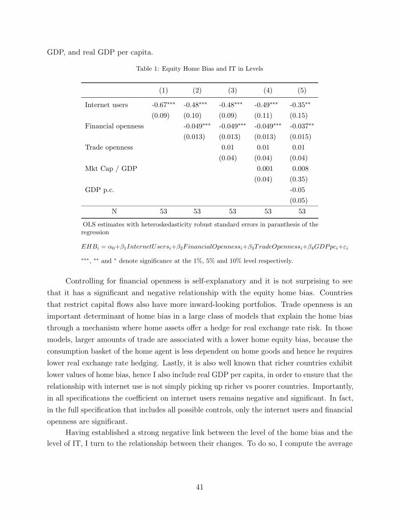
2 Motivating Empirical Evidence
It is well established that aggregate equity portfolios are heavily biased towards domestic
assets. For example, at the end of 2008 the average share of foreign assets in portfolios across
the world was just one third of what it should be under the CAPM (Coeurdacier and Rey
(2013)). This high overall level of home bias has been a long-standing puzzle in international
finance ever since it was first documented by French and Poterba (1991), and has sparked
a large and active literature. In this section, I emphasize that in addition to having a high
6
overall level, the home bias also exhibits a clear downward trend, and has decreased by about
a third since 1995. While much less attention has been paid to this trend, it is a salient
feature of the data as well, and a comprehensive explanation of the home bias phenomenon
should account for both its level and secular decline.
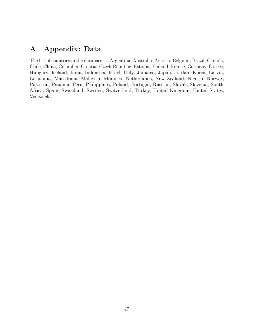
I work with an annual data set of 52 countries for the time period from 1976 to 2015,
that I have compiled with data from the IMF and the World Bank.6 I have included all
countries for which there is an extensive amount of portfolio data available, with the exception
of small countries that are also major international financial centers like Luxembourg and
Singapore. The data set is fairly comprehensive, and covers both developing and developed
countries – thirty-one of the countries, about 60% of the total, are members of the OECD.
The complete list of countries and other details about the data set are in the Appendix.
To quantify the home bias, I follow the literature and measure it as the deviation from
the market portfolio, and define the Equity Home Bias (EHB) index:
EHBi = 1− Share of Foreign Assets in Country i’s Portfolio
Share of Foreign Assests in World Portfolio
This index is zero when the share of foreign assets in country i’s portfolio is equal to their
corresponding share in the market portfolio, and is positive when the portfolio over-weights
domestic assets, and thus exhibits home bias. In the extreme case where the portfolio is
composed exclusively of domestic assets, it is equal to 1.
The home bias is clearly a pervasive feature of the data both across time and across
countries. All country-year pairs exhibit a positive EHB index, and the average value across
time and countries is 0.8, which signifies that the average share of foreign assets over that
time period was just 20% of the CAPM benchmark. Moreover, the standard deviation of the
average EHB across countries is just 0.07.
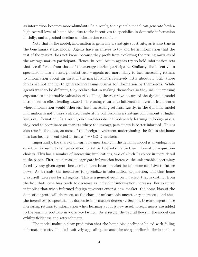
Such statistics speak to the remarkably high overall level of the home bias, but mask
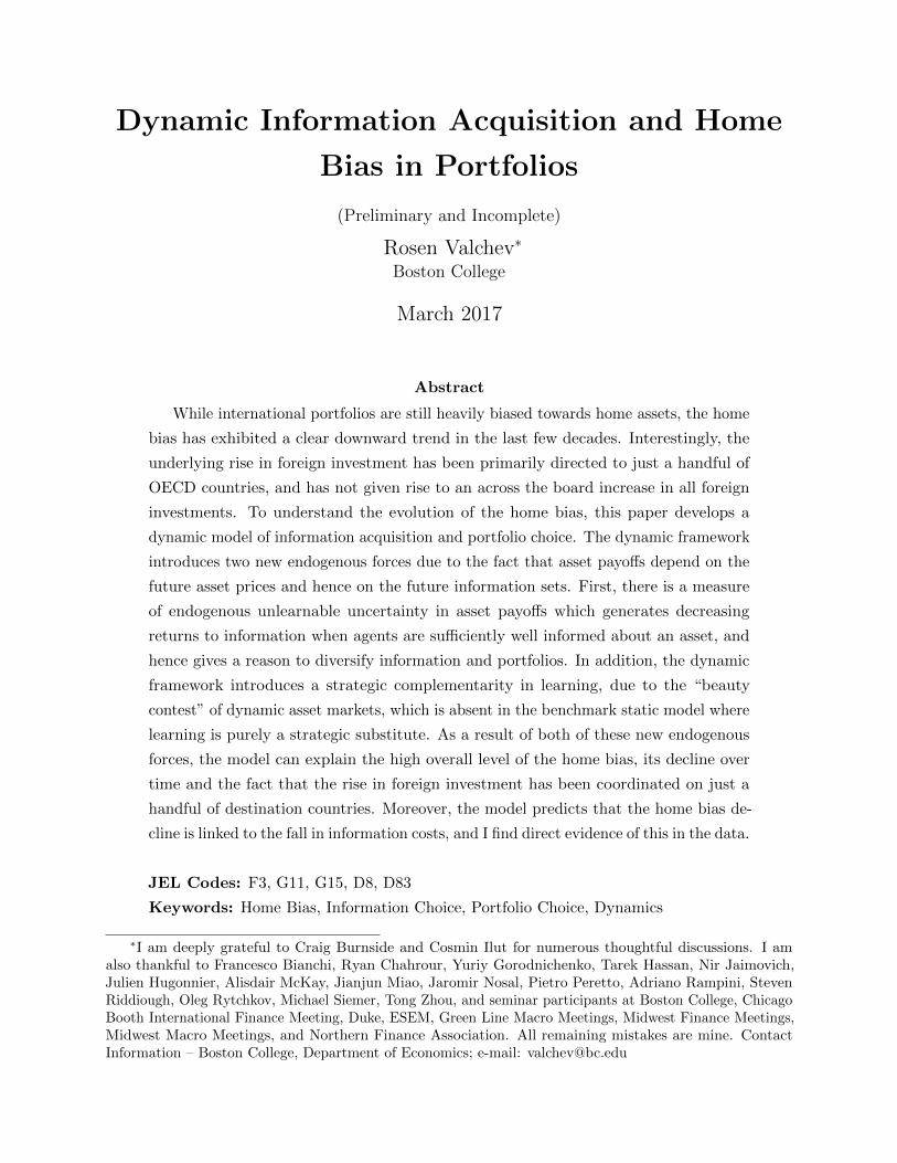
the fact that it has also exhibited a very interesting evolution over time. To illustrate this,
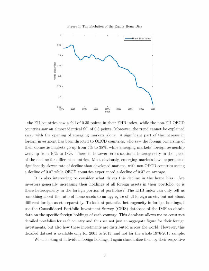
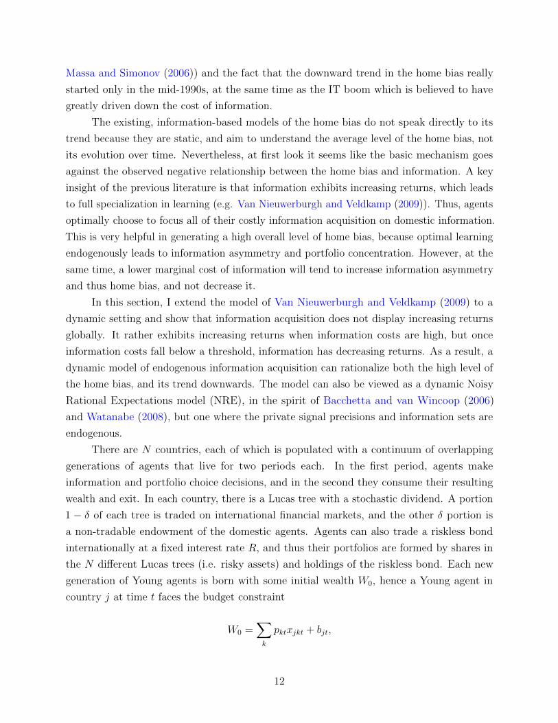
Figure 1 plots the average EHB for the fifty-three countries across time. The downward trend
is very clear. The average home bias was roughly 0.93 in 1976, but has fallen all the way
down to 0.65 by 2015. In other words, the share of foreign assets has went from being ten
times smaller than the CAPM benchmark, to three times smaller. Thus, even though the
home bias is still very much a puzzle today, it has also experienced a remarkable downward
trend and has declined by about a third (as measured by the EHB index).
The decline is a very robust feature of the data, with virtually every single country
experiencing a fall in the EHB index in the last two decades. It is not simply a EU effect
6For a smaller subset of countries, the data can be extended back to 1976 and the results on the generaldownward trend of the home bias remain the same.
7
Figure 1: The Evolution of the Equity Home Bias
Year1975 1980 1985 1990 1995 2000 2005 2010 2015
Hom
e B
ias
Inde
x
0.65
0.7
0.75
0.8
0.85
0.9
0.95
1
Home Bias Index
– the EU countries saw a fall of 0.35 points in their EHB index, while the non-EU OECD
countries saw an almost identical fall of 0.3 points. Moreover, the trend cannot be explained
away with the opening of emerging markets alone. A significant part of the increase in
foreign investment has been directed to OECD countries, who saw the foreign ownership of
their domestic markets go up from 5% to 38%, while emerging markets’ foreign ownership
went up from 10% to 18%. There is, however, cross-sectional heterogeneity in the speed
of the decline for different countries. Most obviously, emerging markets have experienced
significantly slower rate of decline than developed markets, with non-OECD countries seeing
a decline of 0.07 while OECD countries experienced a decline of 0.37 on average.
It is also interesting to consider what drives this decline in the home bias. Are
investors generally increasing their holdings of all foreign assets in their portfolio, or is
there heterogeneity in the foreign portion of portfolios? The EHB index can only tell us
something about the ratio of home assets to an aggregate of all foreign assets, but not about
different foreign assets separately. To look at potential heterogeneity in foreign holdings, I
use the Consolidated Portfolio Investment Survey (CPIS) database of the IMF to obtain
data on the specific foreign holdings of each country. This database allows me to construct
detailed portfolios for each country and thus see not just an aggregate figure for their foreign
investments, but also how these investments are distributed across the world. However, this
detailed dataset is available only for 2001 to 2013, and not for the whole 1976-2015 sample.
When looking at individual foreign holdings, I again standardize them by their respective
8
CAPM weights, and define the bias in each individual foreign holding as
Foreign Biasij =Country j’s share in foreign holdings of Country i
Contry j’s share in foreign portion of world portf.− 1 (1)
The index Foreign Biasij measures how over- or under-weighted are country j assets
in the foreign portfolio of country i. If the index is positive, this means that country i is
over-weighing its investments into country j, as compared to the CAPM, and vice versa.
Note that the index is specifically defined on the foreign portfolio of each country, and not
on its portfolio as a whole. This is because as we know the overall portfolio is heavily biased
towards home assets, and thus all foreign assets are under-weighted against CAPM. But it
is still interesting to ask what foreign assets are more or less over-weighted relative to each
other, and hence the index in (1).
A few interesting results emerge. First, the distribution of foreign holdings of countries
exhibits large fat right tails. The great majority of foreign holdings are held in roughly the
same proportions, but a few are heavily over-weighted, and represent large positive outliers.
The average kurtosis of the distributions of all fifty-three countries in my data set is 23.4 and
the average skewness is 4.
In terms of the evolution of foreign holdings over time, most barely change at all, but a
few experience large shifts. The large movers are roughly equally distributed among negative
and positive shifts, thus foreign portfolios have seen both some assets increase a lot in weight,
and other decrease a lot, while most remain virtually unchanged. More specifically, the
distribution of changes in Foreign Biasit again exhibits fat tails with an average kurtosis of
26, and generally 92% of the changes in Foreign Biasit are less than 0.1. Lastly, those few big
movers in each portfolio, are not all the same across the portfolios of all countries.
Most interestingly, the majority of the overall increase in foreign assets since 2001 has
come due to the few investments that have experienced large shifts in their individual bias.
Thus, for the average country, the increase in foreign assets has come about not due to a
broad increase in foreign holdings, but primarily due to shifts in the holdings of a few of its
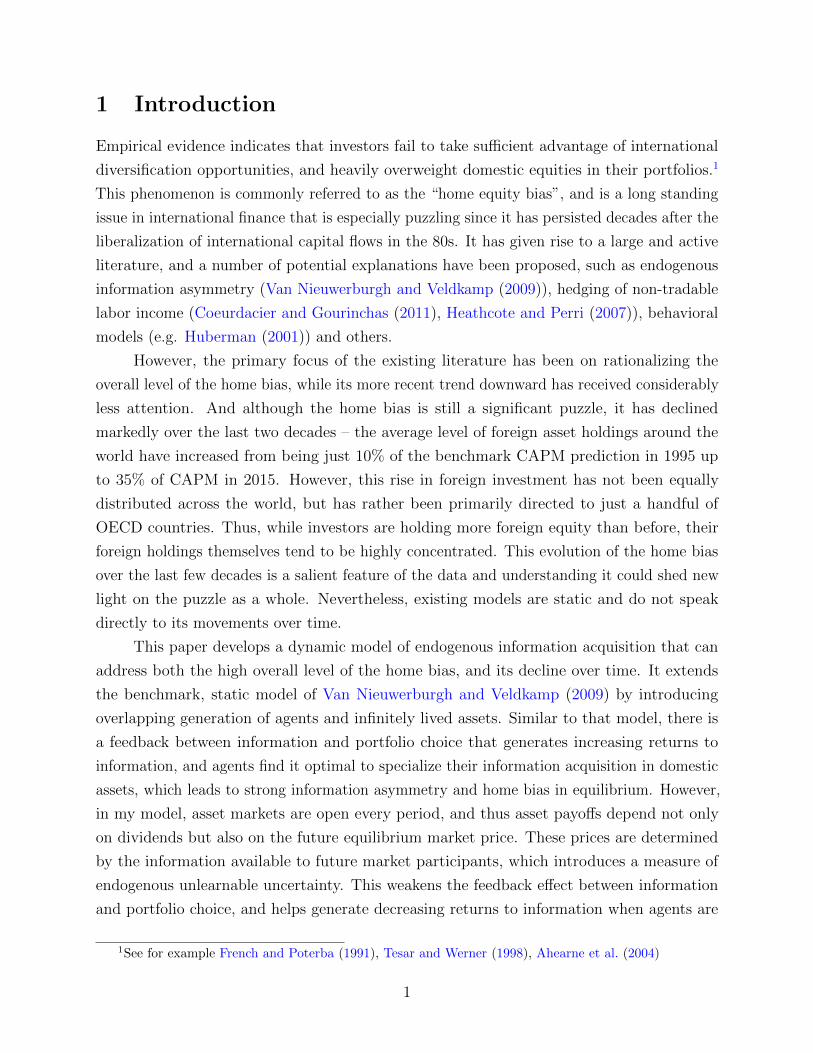
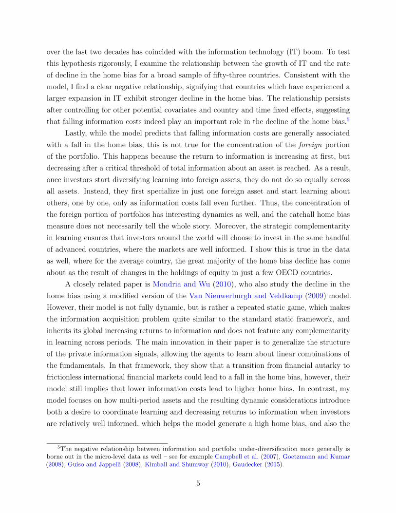
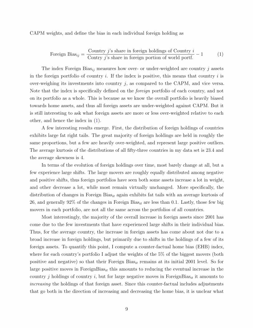
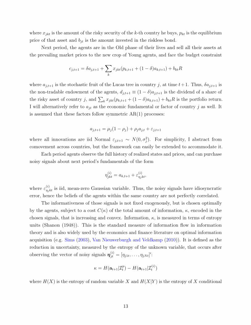
foreign assets. To quantify this point, I compute a counter-factual home bias (EHB) index,
where for each country’s portfolio I adjust the weights of the 5% of the biggest movers (both
positive and negative) so that their Foreign Biasit remains at its initial 2001 level. So for
large positive moves in ForeignBiasit this amounts to reducing the eventual increase in the
country j holdings of country i, but for large negative moves in ForeignBiasit it amounts to
increasing the holdings of that foreign asset. Since this counter-factual includes adjustments
that go both in the direction of increasing and decreasing the home bias, it is unclear what
9
would be the overall effect on the counter-factual EHB index.
Figure 2: Counter-Factual Home Bias
2000 2002 2004 2006 2008 2010 2012 2014
Year
0.55
0.6
0.65
0.7
0.75
0.8
Hom
e B
ias
Inde
x Actual Home Bias
Counterfactual Home Bias
The resulting counter-factual EHB index (again averaged over all countries) is plotted
in Figure 2. The figure shows that the bulk of the reduction in the home bias has come about
as the result of just a handful of big movers in foreign holdings, and not as a broad-based
increase in foreign assets. In particular, 84% of the decline in the home bias between 2001 and
2013 is due to the 10% biggest movers in foreign holdings (again both positive and negative
moves have been included). In particular, if we adjust the holdings of the 10% of biggest
movers, so that they do not change their ForeignBiasit index, then the home bias would have
decreased by just 0.03 points on average between 2001-2013, but in fact it has decreased by
0.16 points. Thus, we see that relying on the EHB index by itself is hiding some interesting
heterogeneity in the trends of specific foreign investments. The fall in the home bias has
happened due to the rapid increase in holdings of a few foreign assets in each portfolio, and
not because of a general increase in all foreign assets.
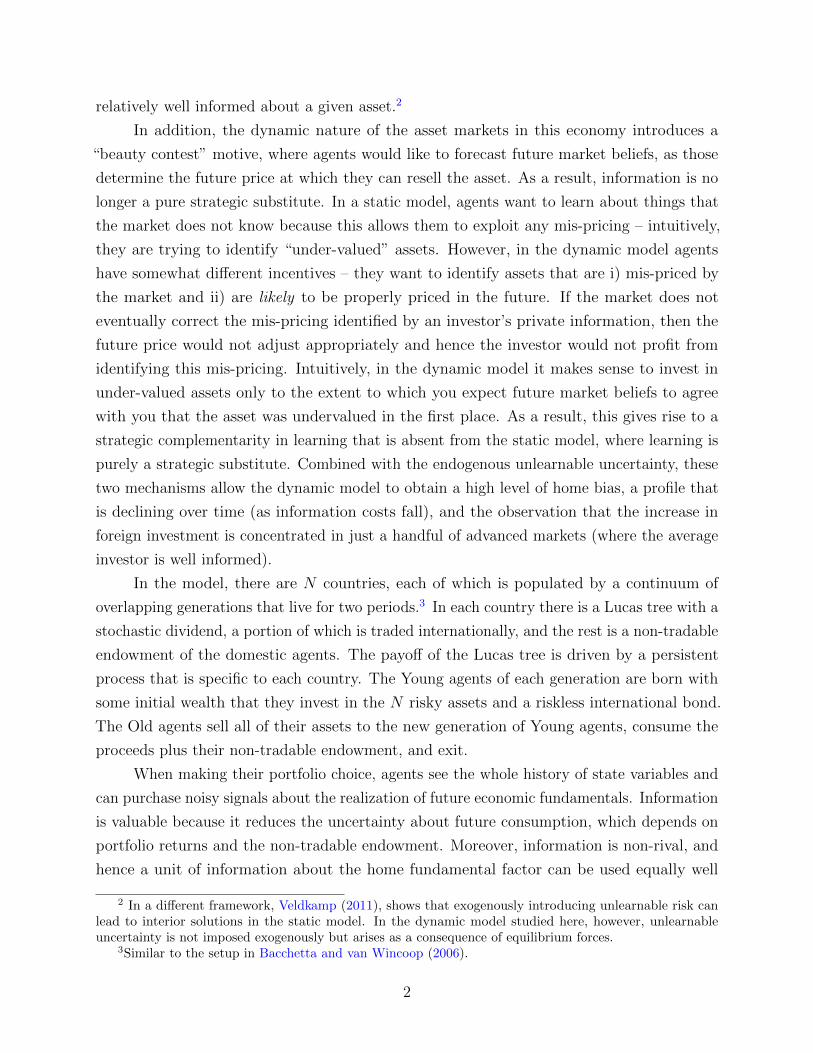
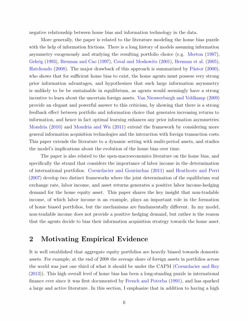
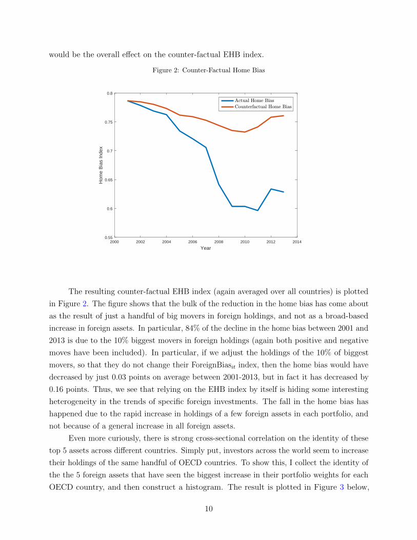
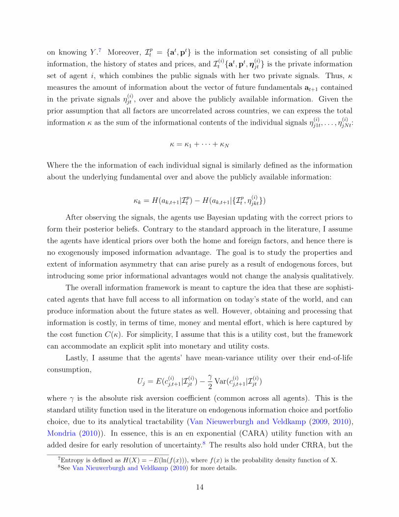
Even more curiously, there is strong cross-sectional correlation on the identity of these
top 5 assets across different countries. Simply put, investors across the world seem to increase
their holdings of the same handful of OECD countries. To show this, I collect the identity of
the the 5 foreign assets that have seen the biggest increase in their portfolio weights for each
OECD country, and then construct a histogram. The result is plotted in Figure 3 below,
10
and show that the increase in investment underlying the drop in the home bias has been
disproportionately directed to just a few OECD countries, with the US, UK, France and
Germany being one of the most popular destinations.
Figure 3: Distribution of the TOP 5 foreign holdings
Aus
tral
iaA
ustr
iaB
elgi
umB
razi
lB
ulga
riaC
anad
aC
zech
Rep
ublic
Den
mar
kF
inla
ndF
ranc
eG
erm
any
Gre
ece
Hun
gary
Irel
and
Italy
Japa
nN
ethe
rland
sN
ew Z
eala
ndN
orw
ayR
oman
iaS
erbi
aS
pain
Sw
eden
Sw
itzer
land
Tun
isia
Ukr
aine
Uni
ted
Kin
gdom
Uni
ted
Sta
tes
0
5
10
15
20
25
Overall, the trend downward is clearly an important, robust feature of the data, that
goes beyond the opening up of emerging markets and lifting of capital restrictions. However,
the underlying increase in foreign investment has not been spread around the world, but has
been heavily concentrated in OECD markets. Understanding these facts can help discipline
models of the home bias, and help us better understand the puzzle as a whole.
3 The Model
In this section I turn towards a model that can explain not only the high overall level of the
home bias, but also its decline and the fact that underlying = increase in foreign investment
has been directed to just a handful of developed markets. I will in particular consider working
with a model of information frictions, where the home bias arises due to agents finding it
optimal to be better informed about home as opposed to foreign information. I am motivated
to work with information models due to abundant evidence that information frictions are
important empirical determinants of the home bias (see Ahearne et al. (2004), Amadi (2004),
11
Massa and Simonov (2006)) and the fact that the downward trend in the home bias really
started only in the mid-1990s, at the same time as the IT boom which is believed to have
greatly driven down the cost of information.
The existing, information-based models of the home bias do not speak directly to its
trend because they are static, and aim to understand the average level of the home bias, not
its evolution over time. Nevertheless, at first look it seems like the basic mechanism goes
against the observed negative relationship between the home bias and information. A key
insight of the previous literature is that information exhibits increasing returns, which leads
to full specialization in learning (e.g. Van Nieuwerburgh and Veldkamp (2009)). Thus, agents
optimally choose to focus all of their costly information acquisition on domestic information.
This is very helpful in generating a high overall level of home bias, because optimal learning
endogenously leads to information asymmetry and portfolio concentration. However, at the
same time, a lower marginal cost of information will tend to increase information asymmetry
and thus home bias, and not decrease it.
In this section, I extend the model of Van Nieuwerburgh and Veldkamp (2009) to a
dynamic setting and show that information acquisition does not display increasing returns
globally. It rather exhibits increasing returns when information costs are high, but once
information costs fall below a threshold, information has decreasing returns. As a result, a
dynamic model of endogenous information acquisition can rationalize both the high level of
the home bias, and its trend downwards. The model can also be viewed as a dynamic Noisy
Rational Expectations model (NRE), in the spirit of Bacchetta and van Wincoop (2006)
and Watanabe (2008), but one where the private signal precisions and information sets are
endogenous.
There are N countries, each of which is populated with a continuum of overlapping
generations of agents that live for two periods each. In the first period, agents make
information and portfolio choice decisions, and in the second they consume their resulting
wealth and exit. In each country, there is a Lucas tree with a stochastic dividend. A portion
1 − δ of each tree is traded on international financial markets, and the other δ portion is
a non-tradable endowment of the domestic agents. Agents can also trade a riskless bond
internationally at a fixed interest rate R, and thus their portfolios are formed by shares in
the N different Lucas trees (i.e. risky assets) and holdings of the riskless bond. Each new
generation of Young agents is born with some initial wealth W0, hence a Young agent in
country j at time t faces the budget constraint
W0 =∑k
pktxjkt + bjt,
12
where xjkt is the amount of the risky security of the k-th country he buys, pkt is the equilibrium
price of that asset and bjt is the amount invested in the riskless bond.
Next period, the agents are in the Old phase of their lives and sell all their assets at
the prevailing market prices to the new crop of Young agents, and face the budget constraint
cj,t+1 = δaj,t+1 +∑k
xjkt(pk,t+1 + (1− δ)ak,t+1) + bktR
where aj,t+1 is the stochastic fruit of the Lucas tree in country j, at time t+1. Thus, δaj,t+1 is
the non-tradable endowment of the agents, dj,t+1 ≡ (1− δ)aj,t+1 is the dividend of a share of
the risky asset of country j, and∑
k xjkt(pk,t+1 + (1− δ)ak,t+1) + bktR is the portfolio return.
I will alternatively refer to ajt as the economic fundamental or factor of country j as well. It
is assumed that these factors follow symmetric AR(1) processes:
aj,t+1 = µj(1− ρj) + ρjaj,t + εj,t+1
where all innovations are iid Normal εj,t+1 ∼ N(0, σ2j ). For simplicity, I abstract from
comovement across countries, but the framework can easily be extended to accommodate it.
Each period agents observe the full history of realized states and prices, and can purchase
noisy signals about next period’s fundamentals of the form
η(i)jkt = ak,t+1 + ε
(i)ηjkt
,
where ε(i)ηjkt
is iid, mean-zero Gaussian variable. Thus, the noisy signals have idiosyncratic
error, hence the beliefs of the agents within the same country are not perfectly correlated.
The informativeness of those signals is not fixed exogenously, but is chosen optimally
by the agents, subject to a cost C(κ) of the total amount of information, κ, encoded in the
chosen signals, that is increasing and convex. Information, κ, is measured in terms of entropy
units (Shanon (1948)). This is the standard measure of information flow in information
theory and is also widely used by the economics and finance literature on optimal information
acquisition (e.g. Sims (2003), Van Nieuwerburgh and Veldkamp (2010)). It is defined as the
reduction in uncertainty, measured by the entropy of the unknown variable, that occurs after
observing the vector of noisy signals η(i)jt = [ηj1t, . . . , ηjNt]
′:
κ = H(at+1|Ipt )−H(at+1|I(i)t )
where H(X) is the entropy of random variable X and H(X|Y ) is the entropy of X conditional
13
on knowing Y .7 Moreover, Ipt = {at,pt} is the information set consisting of all public
information, the history of states and prices, and I(i)t {at,pt,η
(i)jt } is the private information
set of agent i, which combines the public signals with her two private signals. Thus, κ
measures the amount of information about the vector of future fundamentals at+1 contained
in the private signals η(i)jt , over and above the publicly available information. Given the
prior assumption that all factors are uncorrelated across countries, we can express the total
information κ as the sum of the informational contents of the individual signals η(i)j1t, . . . , η
(i)jNt:
κ = κ1 + · · ·+ κN
Where the the information of each individual signal is similarly defined as the information
about the underlying fundamental over and above the publicly available information:
κk = H(ak,t+1|Ipt )−H(ak,t+1|{Ipt , η(i)jkt})
After observing the signals, the agents use Bayesian updating with the correct priors to
form their posterior beliefs. Contrary to the standard approach in the literature, I assume
the agents have identical priors over both the home and foreign factors, and hence there is
no exogenously imposed information advantage. The goal is to study the properties and
extent of information asymmetry that can arise purely as a result of endogenous forces, but
introducing some prior informational advantages would not change the analysis qualitatively.
The overall information framework is meant to capture the idea that these are sophisti-
cated agents that have full access to all information on today’s state of the world, and can
produce information about the future states as well. However, obtaining and processing that
information is costly, in terms of time, money and mental effort, which is here captured by
the cost function C(κ). For simplicity, I assume that this is a utility cost, but the framework
can accommodate an explicit split into monetary and utility costs.
Lastly, I assume that the agents’ have mean-variance utility over their end-of-life
consumption,
Uj = E(c(i)j,t+1|I
(i)jt )− γ
2Var(c
(i)j,t+1|I
(i)jt )
where γ is the absolute risk aversion coefficient (common across all agents). This is the
standard utility function used in the literature on endogenous information choice and portfolio
choice, due to its analytical tractability (Van Nieuwerburgh and Veldkamp (2009, 2010),
Mondria (2010)). In essence, this is an en exponential (CARA) utility function with an
added desire for early resolution of uncertainty.8 The results also hold under CRRA, but the
7Entropy is defined as H(X) = −E(ln(f(x))), where f(x) is the probability density function of X.8See Van Nieuwerburgh and Veldkamp (2010) for more details.
14
mean-variance function is more convenient for showing the results cleanly.
3.1 Portfolio Choice and Asset Market Equilibrium
After observing their private signals and updating beliefs, agents form their optimal portfolios.
In doing so, they need to forecast the risky asset payoffs, pk,t+1 + dk,t+1. Dividends, dk,t+1 =
(1−δ)ak,t+1, are Gaussian by assumption, and I conjecture and later verify that the equilibrium
prices pkt are linear in the state variables, and hence are Gaussian as well. Thus, the posterior
beliefs of the agents follow a Normal distribution, which leads to the familiar mean-variance
optimal portfolio holdings:
x(i)jjt =
E(pj,t+1 + dj,t+1|I(i)j )− pjtR
γ Var(pj,t+1 + dj,t+1|I(i)j )
−Cov(δaj,t+1, pj,t+1 + dj,t+1|I(i)
j )
Var(pj,t+1 + dj,t+1|I(i)j )
x(i)jkt =
E(pk,t+1 + dk,t+1|I(i)j )− pktR
γ Var(pk,t+1 + dk,t+1|I(i)j )
where x(i)jkt is the amount of the risky asset k, that the i-th agent in the j-th country
buys. There are two motives for buying the risky assets – a speculative one and a hedging one.
For speculative purposes, agents like to buy assets that offer high expected excess returns and
not too much variance. In addition, the home asset (xjjt) is also useful for hedging the risk
coming from non-tradable income – this is captured by the term −Cov(δaj,t+1,pj,t+1+dj,t+1|I(i)j )
Var(pj,t+1+dj,t+1|I(i)j )
.
Two forces could potentially affect the agent’s desire to alter her portfolio holdings from being
split equally between all available assets. One is the additional hedging motive to trade the
home asset, and the other is any potential information asymmetry, Var(pj,t+1 + dj,t+1|I(i)j ) 6=
Var(pk,t+1 + dk,t+1|I(i)j ) for j 6= k, which would alter the speculative portion of the portfolios.
In addition to the informed traders, each risky asset is also traded by a measure of
“noise” traders, which trade for reasons exogenous to the model. The net noise trader demand
for asset k is zkt ∼ iidN(0, σ2z). Market clearing requires that the sum of the informed agents
trades and the noise traders equals the asset supply, zk, and thus for each asset we have the
market clearing condition
zk + zkt =1
N
∑j
∫x
(i)jktdi (2)
I look for a linear stationary equilibrium where equilibrium prices are time-invariant, linear
functions of the state variables. Because of the linear-Gaussian information structure,
conditional expectation, and hence also portfolio holdings, are linear in the information sets
15
of the agents. Furthermore, given that the market clearing condition (2) sums over these
asset demands, it is perhaps unsurprising that equilibrium prices turn out to be linear in the
aggregate information set:
IAggt = {at,pt, at+1, zt}
This is the information set of a hypothetical social planner that is able to aggregate
the information sets of all individual agents. It includes the actual realizations of the future
fundamentals ak,t+1 because the noise in the private signals of the agents is iid, and hence
aggregating over them perfectly reveals the future fundamentals. Moreover, notice that if an
agent knew the value of ak,t+1, then he would be able to also invert the equilibrium prices,
and uncover the measure of noise traders zkt. Thus, the aggregate information set contains
both the future fundamentals, and the current measure of noise traders, both of which are
unknown to any single investor.
Furthermore, given that the fundamental processes and the noise traders are assumed
to be independent across countries, it turns out that each equilibrium price is a function of
only domestic variables and takes the form,
pkt = λk + λakakt + λakak,t+1 + λzkzkt,
where the coefficients λk, λak, λak, λzk are determined by the market clearing conditions.
Given this, we can explicitly compute the expected payoffs,
µ(i)jkt = E(pk,t+1 + dk,t+1|I(i)
jt ) = λ+ (1− δ + λak + λakρa)︸ ︷︷ ︸≡Λk
E(ak,t+1|I(i)jt )
where I define the variable Λk as the loading of the asset payoff onto the unknown future
fundamental ak,t+1. Similarly, the conditional variance is
Var(pk,t+1 + dk,t+1|I(i)jt ) = Λ2
k Var(ak,t+1|I(i)jt ) + λakσ
2a + λzkσ
2z (3)
The conditional expectation and variance of the future fundamental ak,t+1 follows the
standard formulas for updating Gaussian variables with Gaussian signals. The agents have
two sources of signals, the idiosyncratic signal η(i)jkt, and the equilibrium price itself contains
the signal pkt = ak,t+1 + λakλzkzkt, which they combine with their prior knowledge of akt to
compute,
E(ak,t+1|I(i)jt ) = σ2
kt
(ρaak,tσ2a
+λ2ak
λ2zkσ
2z
(ak,t+1 +
λakλzk
zkt
)+
1
σ2ηjk
ηjkt
)
16
and the posterior variance:
σ2kt = Var(ak,t+1|I(i)
jt ) =
(1
σ2a
+λ2ak
λ2zkσ
2z
+1
σ2ηjk
)−1
Plugging everything back in (2) gives us the solution for the coefficients of the equilibrium
prices. The details are given in the Appendix, and here I will just focus on the coefficients
λak and λzk which determine the relative informativeness of the price as a signal about future
fundamentals. The solutions for those two coefficients are:
λak =1
Rσ2kqk
(1 +
φkqkγ2σ2
z
)λzk = − 1
Rγσ2
k
(1 +
φkqkγ2σ2
z
)where I define σ2
k as the average market participant’s posterior variance of the return of
the k-th asset, which is given by
σ2k =
(1
N
∑j
1
Varjk(pk,t+1 + dk,t+1)
)−1
and qk is the following weighted average of the precisions of all market participants,
qk =∑j
1
N
Λkσ2jkt
Λ2kσ
2jk + λ2
akσ2a + λ2
zkσ2z
1
σ2ηjk
and φk is given by
φk =1
N
∑j
Λkσ2jk
Varjk(pk,t+1 + dk,t+1)=
1
N
∑j
Λkσ2jk
Λ2kσ
2jk + λ2
akσ2a + λ2
zkσ2z
To gain more intuition, note that we can re-write λak as
λak =1
RΛk(1−
φkσ2k
Λkσ2a
)
and thatφkσ
2k
Λkrepresents the average market participants posterior variance over the
unknown fundamental ak,t+1. Thus, in the limit of no private information, when everyone’s
beliefs equal their priors (σ2a), we have λak = 0. Since no one has any information about
the future ak,t+1, its value is not compounded into the equilibrium price today. In the
17
other extreme, when everyone has perfect foresight and the fundamental is fully revealed,
λak = 1R
Λk, which implies that movements in ak,t+1 are priced perfectly, and trading on it
offers just the risk-free return R.9
Lastly, note that even though agents can receive signals about all future fundamental
shocks, there is a measure of “unlearnable” uncertainty that arises endogenously in the
model. That is, the posterior variance of the asset payoffs, equation (6), is not a exclusively
a function of the posterior variance of ak,t+1, which the agents can decrease through costly
information acquisition. In particular, the posterior variance of the payoffs also includes the
terms λ2akσ
2a + λ2
zkσ2z , which represent shocks that the agents cannot learn about. These are
news that realize in the future, and are outside of the scope of today’s information – they
represent “unlearnable uncertainty” to today’s agents.
It is important to note that this unlearnable uncertainty arises endogenously, as a result
of the recursive nature of the dynamic model. The key is that that future information sets are
naturally always one step ahead of today’s information sets. Agent’s private signals contain
news about the one step-ahead fundamental, meaning that today’s agents receive information
about ak,t+1, and that next period’s agents receive information about ak,t+2. This extra
information is incorporated in tomorrow’s prices, since it affects the t+ 1 asset demands, and
thus next period’s equilibrium price pk,t+1 depends on the innovations at time t+ 2:
Hence, today’s agents face some unlearnable uncertainty in the future valuation of the
asset, pk,t+1, and that’s because the information available to them today does not fully span
the market beliefs tomorrow. The two-step ahead innovations are news that are realized in
the future, and are thus outside of the scope of learning of today’s agents. This is a reflection
of the fact that information sets are recursive, and grow over time:
IAggt ⊂ IAggt+1 and IAggt+1 \IAggt 6= ∅
Since, IAggt is coarser than IAggt+1 , the future aggregate information set IAggt+1 contains
uncertainty that is unlearnable for agents at time t. Note that this is not a result of assuming
that agents can only learn about fundamentals one period ahead. If they could learn about
both ak,t+1 and ak,t+2, for example, then next periods information sets would still contain the
9As is known, the equilibrium in the dynamic NRE models is not necessarily unique. In fact, there canbe up to 2k different equilibria – see Watanabe (2008). For most of the analytical result, the equilibriumselection does not matter. For numerical results, as is standard I will focus on the “low volatility” equilibrium,which is the unique stable one.
18
unlearnable εak,t+3. More generally, even if agents had access to information about any future
period, up to some arbitrary T <∞, then the next period’s price would contain unlearnable
information about ak,t+T+1, which would again be outside of today’s scope of learning. In
other words, in any recursive dynamic model, next period’s agents are always one step-ahead
of today’s agents, and hence the information available today does not span the information
tomorrow, and hence does not fully span future market beliefs. As a result, agents always
face some measure of unlearnable valuation risk.
3.2 Information Choice
Agents choose the precision of their signals ex-ante, at the beginning of the period, after
they observe the value of the fundamentals today at, but before receiving the private signals
and asset markets open. Recall that the information carries a cost C(κ), where κ is the
total amount of information encoded in the agent’s private signals (suppressing subscripts to
reduce clutter)
κ = H(at+1|Ipt )−H(at+1|I(i)t )
First, note that I am implicitly assuming that the information encoded in the prices
(and any other public signals) is free, and agents need to pay only for information over and
above that. This is the typical Grossman assumption, but could be easily relaxed. Moreover,
since all elements of the vector at+1 are independent, we can write the above constraint as
κ=
∑k
H(ak,t+1|Ipt )−H(ak,t+1|I(i)t ) =
∑k
κk
where I have defined κk ≡ H(ak,t+1|Ipt )−H(ak,t+1|I(i)t ) as the amount of information purchased
for each individual fundamental ak,t+1. Given the Gaussian structure of the problem, the
entropy has a convenient closed form expression, which is simply the reduction in log variance
from observing the private signal:
κjkt = ln(Var(ak,t+1|Ipt ))− ln(σ2jk)
Then, the agent chooses a combination of κk to maximize ex-ante expected utility
maxκ1,...,κN
E(Uj(x∗t )|at)− C(
∑k
κk)
s.t.
κk ≥ 0
19
The goal of the agent is to maximize his expected utility, knowing that after his signals
realize, he will update his beliefs accordingly, and will optimally choose the portfolio x∗t .
Finally, the non-negativity constraint is a “no forgetting constraint”, meaning that the
agent cannot choose to obtain “negative” information about one of the assets, which will be
equivalent to “loosing” information from one of its priors.
The first main result is to confirm that the information choice is indeed time-invariant,
which would validate our earlier assumption that the equilibrium prices are time-invariant
functions of the state variables. The result is formalized in the proposition below.
Proposition 1. The optimal allocation of information is time-invariant, i.e. κjkt = κjk for
all j, k and t.
Proof. Intuition is sketched out in the text, and details are in the Appendix.
This result tells us that at any time period t, the currently young generation (of country
j) allocates its finite information capacity in the same way that next period’s generation
would do, and last period’s did as well. Thus, the posterior variance of the average market
participant is time-invariant. Going back to the formulas for the equilibrium price coefficients
given above, we see that this guarantees that they do not change over time either.
To gain intuition about the result, it’s useful to derive the ex-ante expected utility that
enters the information choice. I do so for the agent living in country j, and will suppress all
resulting j subscripts to reduce clutter.
E(U(x∗t )|at) = W0R + δρaajt +1
2γ
∑k
Var(exk,t+1|at) + (E(exk,t+1|at))2
Λ2kσ
2k + λ2
akσ2a + λ2
zkσ2z
−(δE(exj,t+1|at) +
γδ2(λ2ajσ
2a+λ2
zjσ2z)
2Λk)Λjσ
2j
Λ2j σ
2j + λ2
ajσ2a + λ2
zjσ2z
where exk,t+1 = pk,t+1 +dk,t+1−Rpkt is the excess return of the k-th asset. Information enters
the agent’s expected utility in two ways. First, it alters his optimal speculative portfolio,
which is given by the summation in the third term, and it alters his optimal hedging portfolio,
which operates through the last term. From a return maximization perspective, information
about all k assets is symmetric, but only home information helps in forming the hedging
portfolio, and hence the last term is not a summation.
We can then derivate in respect to κk to see what is the marginal benefit of an extra
unit of information about the k-th asset.10 To make the notation less burdensome let
10This is the marginal benefit and not utility, because the marginal utility would also take into accountthe cost function. We turn to that in a second.
20
B = δE(exj,t+1|at) +γδ2(λ2
ajσ2a+λ2
zjσ2z)
2Λk, and then
∂U
∂κkt=
Var(exk,t+1) + E(exk,t+1)2
2γ
Λ2kσk
(Λ2kσ
2k + λ2
akσ2a + λ2
zkσ2z)
2+1k=jB
Λjσ2j
(Λ2j σ
2j + λ2
ajσ2a + λ2
zjσ2z)
2
where I have slightly abused notation and written the ex-ante expectation and variance
without the explicit conditioning on the known history at.
The expression shows three main things – agents like to learn about assets that 1) have
high ex-ante expected excess returns, 2) have ex-ante volatile excess returns, and 3) prefer
learning about the home asset (B > 0). Understanding these effects starts with the fact
that information is non-rival, in the sense that a unit of information can be equally applied
to optimizing one’s returns and to forming a better hedging portfolio. The third effect is
perhaps the easiest one to understand – the home asset does not offer only potentially high
excess returns, but also the benefit of hedging the non-tradable labor income of the agents.
As a result, ceteris paribus, home information is the most valuable, because it can help in
both forming a better speculative portfolio, and a better hedging portfolio.
The fact that agents like to learn about assets with high ex-ante expected excess returns
is also quite straightforward. Those are the assets that are likely to present the most profitable
trading opportunities once markets open and hence are likely to represent a bigger portion of
the total portfolio of the agents. Since information is non-rival, it is better to apply a unit of
information to a big portfolio holding, rather than to a small one, and hence agents want to
maximize learning about assets they expect to be a big part of their portfolios.
On the other hand, agents also like to learn about assets with high ex-ante volatility. Part
of this is again because such assets are more likely to present profitable trading opportunities.
The other reason is that volatile excess returns indicate that the market does not posses good
information about the underlying fundamentals and hence mis-prices it. As a result, when
the fundamentals become revealed next period, the price adjusts to account for it, which
drives volatility in the excess returns. To see this more clearly, note that the realized excess
returns are given by
exk,t+1 = σ2kγ(z + zkt) + σkφk(
εak,t+1
σ2a
+qkγσ2
z
zkt) + λakεak,t+2 + λzzk,t+1 (4)
In general, the returns are high when the innovation to ak,t+1, or noise trader supply zkt,
is above mean and low otherwise, but the sensitivity of the returns to those shocks depend
on the posterior variance as perceived by the average market participant. If the market has
perfect information σ2k → 0, then the excess returns do not respond to movements in the
second term in the equation above. This is because those shocks are known, and properly
21
priced at the rate 1R
today.11 Hence, high volatility indicates that the market leaves some of
the variation in future fundamentals and noise trader shocks mis-priced, and this is the type
of variation private information can help agents exploit.
In particular, the expected excess return is
Et(exk,t+1) = γσ2k(z + zkt) + (σ2
kφk − Λkσ2jk)(
εak,t+1
σ2a
+qkγσ2
z
zkt) +Λkσ
2jk
σ2η
εηkt
This shows that when the agents are better informed than the market, σ2kφk−Λkσ
2jk > 0,
the agent’s expectations correctly time the market. They go up (and the portfolio shares
as well) when the actual excess return is indeed likely to be high and vice versa. Thus,
superior information helps the agent engage in profitably exploiting the pricing mistakes
of the average market participant. But for this to be worthwhile, there must be sufficient
amount of mis-pricing, i.e. you want to learn about volatile assets, where the market price
has not incorporated all of the learnable uncertainty.
Lastly, to show that the information acquisition strategy does not vary over time, we
need to show that the ex-ante expected excess returns and variances are not time-varying.
The ex-ante excess return is given by
E(exk,t+1) = γσ2k
[zj +
δ
N
Λkσ2kk
Λ2kσ
2kk + λ2
akσ2a + λ2
zkσ2z
]Basically, the average excess return on risky assets reflects the compensation agents
require for holding the full supply of the risky asset. When the supply is high, in order for the
markets to clear the expected excess return must be high, so as to incentive the risk-averse
agents to increase their holdings. The net supply of the asset is given by the term
zj +δ
N
Λkσ2kk
Λ2kσ
2kk + λ2
akσ2a + λ2
zkσ2z
which has two components. The first one is just the exogenous supply and the second, is any
extra net supply coming from the hedging demands of the agents in country k. Since the
domestic assets and the non-tradable income are positively correlated, the hedging portfolios
of agents would generally short the domestic assets, and this is demand that needs to be
picked up by the rest of the market. In effect, this increases the total supply of the asset
that needs to be soaked up by the speculative portfolios. Since supply is exogenously fixed
over time, if the information strategy itself does not vary (i.e. σ2jj is time invariant) then
ex-ante expected excess returns do not vary over time either. The details of the proof amount
11Also as shown before λak → 0 as average information increases to perfect foresight.
22
to showing that since the ex-ante excess return is given by the same function each period,
agents have no incentives to vary information acquisition.
On the other hand, the ex-ante variance can be expressed as
Var(exk,t+1) = σ2k
(Λkφk + σ2
k(γ2σ2
z + γqkφk))
+ λ2akσ
2a + λ2
zkσ2z
which shows again that if information choice does not vary over time, then the ex-ante
variance of excess returns do not vary either. And we can again show that there is no incentive
to change information choice.
Also note that information acquisition is a strategic substitute. This can be seen from
the expressions for ex-ante expectations and variances. When the market is well informed
about a particular asset (i.e. σ2k low), then the ex-ante expected excess return and ex-ante
volatility is low, making that asset unappealing to learn about. Thus, agents like to learn
about things that the other agents are generally not well informed about. This is the same
result as in Van Nieuwerburgh and Veldkamp (2009) and others.
Lastly, note that if we combine all of these results, we arrive at the conclusion that in
the symmetric equilibrium (where all asset returns and variances are ex-ante symmetric) we
have home bias in information acquisition. This is essentially due to the dual nature of the
home asset, as both an investment and a hedging vehicle. The result is summarized by the
proposition below.
Proposition 2. If δ > 0 agents in country j optimally chooses κj > κk for all k 6= j, i.e.
they choose to acquire more information about the home fundamentals.
Proof. Follows from symmetry, the fact that information is non-rival, and the positive
correlation between the domestic risky asset and non-tradable domestic income. Details are
in the Appendix.
3.3 Information Specialization
The principal feature of the standard, static models of information and portfolio choice is
increasing returns to information. It incentivizes agents to fully specialize in learning, and
thus only acquire domestic information, which is at the heart of the models’ ability to generate
home bias. In this section, I show that the desire to specialize in the dynamic model is more
nuanced, explain the differences and why they arise.
To understand when and why increasing returns to information obtain, it is useful to
compute the derivative of the marginal benefit of extra information. Full details are given in
23
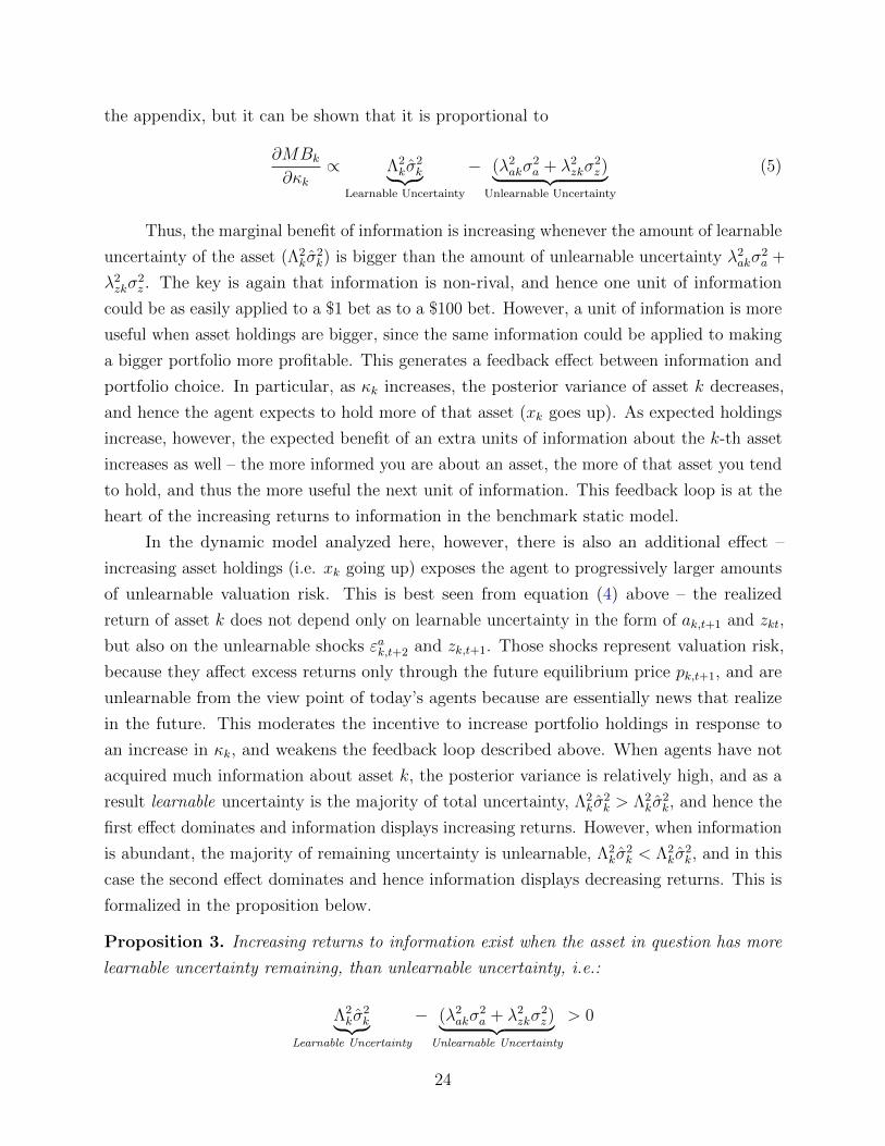
the appendix, but it can be shown that it is proportional to
∂MBk
∂κk∝ Λ2
kσ2k︸ ︷︷ ︸
Learnable Uncertainty
− (λ2akσ
2a + λ2
zkσ2z)︸ ︷︷ ︸
Unlearnable Uncertainty
(5)
Thus, the marginal benefit of information is increasing whenever the amount of learnable
uncertainty of the asset (Λ2kσ
2k) is bigger than the amount of unlearnable uncertainty λ2
akσ2a +
λ2zkσ
2z . The key is again that information is non-rival, and hence one unit of information
could be as easily applied to a $1 bet as to a $100 bet. However, a unit of information is more
useful when asset holdings are bigger, since the same information could be applied to making
a bigger portfolio more profitable. This generates a feedback effect between information and
portfolio choice. In particular, as κk increases, the posterior variance of asset k decreases,
and hence the agent expects to hold more of that asset (xk goes up). As expected holdings
increase, however, the expected benefit of an extra units of information about the k-th asset
increases as well – the more informed you are about an asset, the more of that asset you tend
to hold, and thus the more useful the next unit of information. This feedback loop is at the
heart of the increasing returns to information in the benchmark static model.
In the dynamic model analyzed here, however, there is also an additional effect –
increasing asset holdings (i.e. xk going up) exposes the agent to progressively larger amounts
of unlearnable valuation risk. This is best seen from equation (4) above – the realized
return of asset k does not depend only on learnable uncertainty in the form of ak,t+1 and zkt,
but also on the unlearnable shocks εak,t+2 and zk,t+1. Those shocks represent valuation risk,
because they affect excess returns only through the future equilibrium price pk,t+1, and are
unlearnable from the view point of today’s agents because are essentially news that realize
in the future. This moderates the incentive to increase portfolio holdings in response to
an increase in κk, and weakens the feedback loop described above. When agents have not
acquired much information about asset k, the posterior variance is relatively high, and as a
result learnable uncertainty is the majority of total uncertainty, Λ2kσ
2k > Λ2
kσ2k, and hence the
first effect dominates and information displays increasing returns. However, when information
is abundant, the majority of remaining uncertainty is unlearnable, Λ2kσ
2k < Λ2
kσ2k, and in this
case the second effect dominates and hence information displays decreasing returns. This is
formalized in the proposition below.
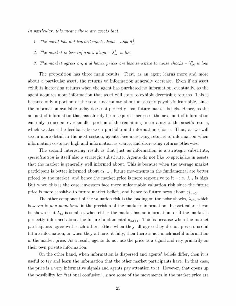
Proposition 3. Increasing returns to information exist when the asset in question has more
learnable uncertainty remaining, than unlearnable uncertainty, i.e.:
Λ2kσ
2k︸ ︷︷ ︸
Learnable Uncertainty
− (λ2akσ
2a + λ2
zkσ2z)︸ ︷︷ ︸
Unlearnable Uncertainty
> 0
24
In particular, this means those are assets that:
1. The agent has not learned much about – high σ2k
2. The market is less informed about – λ2ak is low
3. The market agrees on, and hence prices are less sensitive to noise shocks – λ2zk is low
The proposition has three main results. First, as an agent learns more and more
about a particular asset, the returns to information generally decrease. Even if an asset
exhibits increasing returns when the agent has purchased no information, eventually, as the
agent acquires more information that asset will start to exhibit decreasing returns. This is
because only a portion of the total uncertainty about an asset’s payoffs is learnable, since
the information available today does not perfectly span future market beliefs. Hence, as the
amount of information that has already been acquired increases, the next unit of information
can only reduce an ever smaller portion of the remaining uncertainty of the asset’s return,
which weakens the feedback between portfolio and information choice. Thus, as we will
see in more detail in the next section, agents face increasing returns to information when
information costs are high and information is scarce, and decreasing returns otherwise.
The second interesting result is that just as information is a strategic substitute,
specialization is itself also a strategic substitute. Agents do not like to specialize in assets
that the market is generally well informed about. This is because when the average market
participant is better informed about ak,t+1, future movements in the fundamental are better
priced by the market, and hence the market price is more responsive to it – i.e. λak is high.
But when this is the case, investors face more unlearnable valuation risk since the future
price is more sensitive to future market beliefs, and hence to future news about εak,t+2.
The other component of the valuation risk is the loading on the noise shocks, λzk, which
however is non-monotonic in the precision of the market’s information. In particular, it can
be shown that λzk is smallest when either the market has no information, or if the market is
perfectly informed about the future fundamental ak,t+1. This is because when the market
participants agree with each other, either when they all agree they do not possess useful
future information, or when they all have it fully, then there is not much useful information
in the market price. As a result, agents do not use the price as a signal and rely primarily on
their own private information.
On the other hand, when information is dispersed and agents’ beliefs differ, then it is
useful to try and learn the information that the other market participants have. In that case,
the price is a very informative signals and agents pay attention to it. However, that opens up
the possibility for “rational confusion”, since some of the movements in the market price are
25
caused by noise shocks, zkt, but they get incorrectly interpreted as useful information about
the future fundamentals. It can be shown that this rational confusion amplifies the effects
of the noise shocks on the equilibrium price, and hence increases the value of λ2zk. Thus,
market prices become more sensitive to noise shocks, which increases the valuation risk faced
by agents. The rational confusion effect is strongest for intermediate values of information
dispersion, when the market participants disagree the most.
3.4 Information Costs and Optimal Information Acquisition
In this section I turn to analyzing what happens with information choice and home bias
when the cost of information falls. To start, note that I will say that function C1(.) exhibits
higher information costs than C2(.) if C1(κ) ≥ C2(κ) for all κ > 0. Next, note that the
full information problem can be solved in two steps. First given a fixed amount of total
information κ, the agent chooses the optimal allocation of this information among the different
κk. Second, given that optimal allocation, the agent optimizes over the total amount of
information to purchase κ. The main results of this section are formalized in the two theorems
below.
Proposition 4. Every cost function C(κ) implies a unique optimal total information κ∗.
Moreover, if C ′1(κ) ≥ C ′2(κ) for all κ > 0, then κ∗1 < κ∗2.
Proof. Sketched in the text, details in the Appendix.
The first result is straightforward. Given a convex cost function, there exists a unique
total amount of information that the agent likes to purchase, since at some point the marginal
cost of additional information becomes too high. The second result is also very intuitive, if we
decrease the marginal cost of information, then the optimal quantity of information purchased
will increase (remember that information always displays decreasing returns eventually).
Proposition 5. There exist positive constants {K0 < K1 < · · · < KN−1} such that if
• κ∗ ≤ K0 – agents specialize fully in learning about the domestic asset: κj > 0, κk = 0
for all other k
• κ∗ ∈ (KL−1, KL] – agents learn about home and L > 0 foreign assets: κj > 0, κk′ > 0
for L different k′ 6= j, and κk = 0 for all other k
• κ∗ > KN−1 – agents learn about all assets: κk > 0 for all k.
Moreover, all foreign assets that the agent chooses to learn about receive the same amount of
information acquisition. Thus, for any two k, k′ where κk > 0, κk′ > 0 we have κk = κk′
26
Proof. Sketched in the text, details in the Appendix.
The general intuition for the result follows from the conditions under which information
displays increasing returns. As we saw in Proposition 2, increasing returns obtain when the
agent has not learned much about a particular asset. Moreover, from Proposition 1 we know
that the most preferred asset is the home asset. As a result, when information costs are
relatively high and it is not profitable to acquire much information in total, i.e. κ∗ ≤ K0, the
agent finds it optimal to fully specialize in the home asset. This is the most valuable asset,
and is the one that the scarce information is best used on.
As information costs fall and κ∗ increases, the agent moves into the part of the parameter
space where home information starts exhibiting decreasing returns, and thus eventually finds it
optimal to start acquiring information about foreign assets as well. However, this information
diversification does not happen smoothly across all assets. Rather, at first when κ∗ ∈ (K0, K1],
the agent only acquires information about one foreign asset, then as information costs drop
further he adds a second foreign asset to his learning portfolio and so on. Eventually, when
information costs are low enough, he would be learning about all assets.
Information percolates through the different available assets in this step-wise manner
because this is the best way of economizing on information acquisition costs. Since information
has increasing returns when it is scarce, the agent finds it optimal to specialize whenever
he first starts learning about a particular asset. Thus, when new assets are added to the
learning portfolio the agent fully specializes in them. And as information costs fall further,
at some point he finds it optimal to add a second foreign asset to the learning portfolio, in
which case he specializes in acquiring information in two foreign assets, but none of the other
ones and so on.
The particular structure of the problem implies that the information asymmetry of
home vs foreign information is non-monotonic in information costs. When information costs
are high, the agent fully specializes in home information and does not acquire any foreign
information. In that part of the state space, as information costs fall, the asymmetry is in
fact rising, because the agent invests more and more resources into home information, but
does not acquire any foreign information. But once information costs fall to the point where
κ∗ > K0, the agent starts acquiring foreign information as well, and in fact he starts acquiring
more foreign than home information. As a result, as the information costs fall, the agent
is gradually diversifying his learning into foreign information, and his overall information
asymmetry decreases as well.
Lastly, it is interesting to note that the agent splits the foreign assets into two groups
– those he chooses to learn about and those he chooses not to. If at any point the agent
chooses to learn about more than one foreign asset, then those assets will all receive the same
27
amount of information acquisition. The intuition is that it is only beneficial to learn about
more than one foreign assets when the information costs are low enough so that the agent
has fully exhausted the increasing returns of the first foreign asset. But once he decides to
add a second foreign asset to his learning portfolio, it is again best to fully exhaust the gains
to specialization in that asset immediately as well. And thus, whenever the agent is learning
about two foreign assets he is in fact on an interior solution for information allocation, and
since all foreign assets are symmetric, this results in κk′ = κk for any two foreign assets k′
and k that the agent decides to learn about.
So then even though home vs foreign information asymmetry is falling monotonically
with information costs, the foreign assets are not treated as a homogeneous group that rises
all together. In fact, the agent specializes in a subset of the foreign assets, and completely
ignores the others. As a result, the concentration of the foreign holdings of the agent are in
fact also at first increasing, and then decreasing as information costs fall. That is because
initially the agent specializes learning in just one or two foreign assets, and only eventually
gets around to learning about all foreign assets.
The analysis of this section considered changing the information cost of one agent in a
way that does not affect the information costs faced by the market as a whole. When the
information costs fall in the aggregate (same for everyone), then the sequence of cutoffs {Kl}decrease because the incentives to specialize decrease. This is because when the market as a
whole is better informed, λ2ak is high, the valuation risks are higher and individual agents
find it less desirable to specialize. This is a general equilibrium effect – as the counter-parties
to your trades become more informed, it is less profitable for you to specialize in information
acquisition.
Proposition 6. If the information costs fall for all market participants, then the positive
constants {K0 < K1 < · · · < KN−1} decrease.
3.5 Optimal Portfolios
As a result of the step-wise nature of optimal information acquisition, the optimal portfolio is
formed by three types of assets – the home asset, the foreign assets that the agent does learn
about, and the foreign assets he does not. In fact, this gives rise to a three-fund separation
theorem. In particular, the optimal risky asset portfolio is a convex combination of 1) a fund
holding 100% domestic assets, zj , 2) a fund that is perfectly diversified over the foreign assets
the agent does learn about and holds nothing else, zlearn, and 3) a fund that is perfectly
diversified over the foreign assets he does not learn about zno learn. The aggregate portfolio
28
of country j can be expressed as,
x = αzj + β1zlearn + β2zno learn
This result follows directly from the previous section. The agent always finds it optimal
to learn the most about the home asset, hence there is asymmetry in home vs foreign
information which affects home vs foreign holdings. However, the agent does not treat all
foreign assets symmetrically. There is a subset of assets (possibly empty) that the agent
allocates positive information acquisition to, and the rest of the assets do not receive any
information. The agent treats all foreign assets within each subclass equally, which generates
the three-fund theorem above.
It is interesting to consider how the portfolio holdings are adjusted when information
costs fall. The first and most obvious effect is the “home bias”, which measures the relative
holding of home versus all foreign assets. To quantify the home bias, I will use the same
Equity Home Bias index as in the empirical section, which was defined as:
EHB = 1− Foreign Equity as a Share of the National Portfolio
Foreign Equity as a Share of the World Market Portfolio
The market portfolio is simply the exogenous vector of asset supply
xMKT = z.
This is the CAPM portfolio, and will be the equilibrium portfolio in this model when
there is no learning C(κ) =∞ for all κ > 0, and there is no non-tradable income δ = 0. In
that case, agents are identical across both countries and in equilibrium all hold the market
portfolio, given by the per-capita supply of assets. To illustrate what happens when we
introduce non-tradable income δ > 0 and learning, I will use an example with just two
symmetric countries, a home and a foreign one. When agents have non-tradable income,
δ > 0, but still face infinite information costs, then the equilibrium portfolios become
xNoInfoh = zh −δ
2
σ2a
(1 + λ2a)σ
2a + λ2
zσ2z
xNoInfof = zf +δ
2
σ2a
(1 + λ2a)σ
2a + λ2
zσ2z
where a subscript h denotes the home country and f denotes the foreign country. Compared
to the CAPM portfolio, this one is tilted towards foreign assets due to the hedging motive
introduced by non-tradable income. The portfolios exhibit foreign bias, because of the
negative hedging demand for the home asset. Given symmetry, zh = zf = z, the resulting
29
EHB index value is
EHBNoInfo = 1−xNoInfof
xNoInfoh + xNoInfof
= − δ
2z
σ2a
(1 + λ2a)σ
2a + λ2
zσ2z
It is negative, since the portfolio is biased towards foreign assets. So the hedging channel
by itself is not helping us in generating home bias. It is the information channel that works
in the opposite direction by generating information asymmetry, where agents are better
informed about the home asset. Letting σ2e = λ2
aσ2a + λ2
zσ2z denote the amount of unlearnable
uncertainty agents face, then when agents can acquire information, the resulting optimal
portfolio of the home agent is:
xh = E(
∫(x
(i)h ) =
σ2h
σh + σ2e
[z +
δ
2
σ2h
σ2h + σ2
e
]− δ σ2
h
σ2h + σ2
e
xf = E(
∫(x
(i)f ) =
σ2f
σf + σ2e
[z +
δ
2
σ2f
σ2f + σ2
e
]The resulting EHB is
EHBOptInfo = 1− σ2h
σ2f + σ2
e
− δ
2z
σ2h
σ2f + σ2
e
σ∗2fσ∗2f + σ2
e
The third component is the hedging channel that was already discussed (starred variables
represent the choice variable of the foreign agent), and the second component works through
the informational channel. Since optimal information acquisition is skewed towards the
domestic asset (Proposition 5), then 1− σ2h
σ2f+σ2
e> 0 and thus the second component generates
positive home bias. Moreover, the optimal information acquisition also lowers the negative
effect of the hedging channel, since σ∗2f < σ2a.
Thus, the overall level of the home bias depends on the equilibrium information
asymmetry. It depends on how different is the home agent’s precision over foreign assets,
σ2f , compared to the precision on home assets, σ2
h.12 average market participant’s precision
over domestic assets, σ2h. In turn, Proposition 5 shows that this information asymmetry is
non-monotonic in information costs. As information costs decrease, information asymmetry
is at first increasing, as people further specialize into domestic assets, and then steadily
falls as costs go to zero. The home bias in portfolios, measured by EHB, exhibits the same
non-monotonicity, as illustrated in Figure 4, which is drawn for an economy with five total
12Note that in the formula above the comparison is actually between the precision of the home agenton foreign assets and the precision of the average market participant over home assets. That’s because theformula is for the equilibrium EHB – as home agents acquire more information about home assets, then theoverall market precision over home assets increases, and thus σ2
h goes down.
30
countries (N = 5).
Figure 4: Portfolio Bias and Information Capacity
5* (Information Capacity)
0
Equ
ity H
ome
Bia
s In
dex
(EH
B)
0
Change in Individual Information Cost
End Info ChoiceNo Information<2
e = 0
Figure 4 also hints at another important effect – the increased investment in foreign
assets is not spread out equally across all foreign assets. As we know from Proposition 5, the
agent learns only about a subset of the available foreign assets, and moreover any assets that
he learns about are treated equally. Thus, as information costs fall enough to incentivize the
agent to start acquiring foreign information, at first he only focuses on one of the foreign
assets. As information costs fall sufficiently, he finds it optimal to learn about an additional
foreign asset and so on and so forth.
This can be seen from the discrete drops in the EHB (blue line) as information costs
fall. At first the home bias is falling smoothly, and that’s the region in which the agent is
learning only about the home asset and 1 foreign asset. Then as information costs fall further,
there’s a discrete drop in the home bias, which happens at the point where there agent starts
acquiring information about a second foreign asset. As information at first enjoys increasing
returns, it is never optimal for the agent to learn just a little bit about the new foreign asset,
while still learning a lot about the initial foreign asset he started learning about. Instead,
there’s a discrete jump in the amount of information acquired about this second asset, that
goes from 0 straight to the amount learned about the other foreign asset. Then the agent
keeps investing in acquiring more information about those two foreign assets as information
31
costs fall further, until a point at which he finds it optimal to learn about 3 foreign assets
and etc.
Figure 5: Concentration of Foreign Holdings and Information Capacity
5* (Information Capacity)
0
Bia
s in
For
eign
Por
tfolio
0
Change in Individual Information Cost
Therefore, as information costs and the home bias fall, the foreign portion of the
portfolio is undergoing its own non-monotonic adjustment in concentration, where its own
concentration is at first rising and then falling. When information costs are so high that the
agent only acquires home information, then he holds a under-weighted position in a perfectly
diversified foreign fund. However, as information costs fall and he diversifies learning, the
concentration of the agent’s foreign holdings increases. At first he specializes in one foreign
asset, then in two, three and so on. In the limit, he goes back to a perfectly diversified foreign
fund. Thus, in the parameter space where the home bias (EHB) exhibits a monotonic fall,
the concentration in the foreign portion of portfolios is non-monotonic. This is illustrated in
Figure 5, which plots a concentration index for the foreign holdings of the agents. As we can
see, at first concentration among foreign holdings is increasing, and then it decreases.13
It is also interesting to consider the effect on the non-tradable income. On the one
hand, it generates a negative hedging demand, which is best seen in the fact that the EHB
index for low values of information, κ∗ is negative in Figure 4. On the other, the fact that the
non-tradable income is correlated with the domestic dividends gives the agents an incentive
13It plots the bias index defined as∑
k1
N−1 |Foreign Biasik|, where Foreign Biasik = xik∑k 6=i xik
/ zk∑k 6=i zk
− 1
32
to value home information more than foreign information, and is the reason that agents focus
their learning on home information. Thus, it is a big part of the reason that the EHB index
is initially strongly increasing with κ∗. Figure 6 illustrates this by comparing the resulting
home bias with a model where there is no non-tradable income (δ = 0), but instead agents
have a small information advantage over home information. As we can see, in that case we
can still generate some home bias, due to the initial desire to specialize, but the incentive to
specialize wears off much quicker. As a result, the overall level of the home bias that can be
achieved is much smaller, and comes at a lower level of total information acquired.
Figure 6: Effect of Non-Tradable Income
5* (Information Capacity)
0
Equ
ity H
ome
Bia
s In
dex
(EH
B)
0
No Labor Income
$/ >0$$/ = 0$
Lastly, the comparative static exercises up to this point considered changing the
information costs of just one agent, and keeping the equilibrium unchanged. What happens
if the whole market experiences a fall in information costs? The individual agent effect
described above is still active – at first you increase home bias in information acquisition, and
then you gradually decrease it. However, there is also an additional general equilibrium effect
– as the overall informativeness of the market increases, the gains to specialization decrease.
As a result, it is less profitable to specialize, and investors find it optimal to start diversifying
learning, and hence portfolio holdings, earlier. This is illustrated in Figure 7 below.
It shows the resulting EHB of a single investor for different values of information costs,
at different levels of aggregate market information. The red line displays the case where
33
Figure 7: Portfolio Bias and Information Capacity
0
1/A (1 / Informatino cost )
0
Equ
ity H
ome
Bia
s In
dex
(EH
B)
Aggregate Change in Information Cost
More Agg InformationLess Aggregate Information
the market has less information, and the blue line when it has more information. As the
average market participant becomes more informed, the agent faces increased valuation risk
(through larger λ2ak) and this decreases the desire to specialize through equation (5). Notice
that the overall EHB level is lower at all levels of information acquired by the agent κ∗. This
is because he is facing an increased amount of unlearnable valuation risk, and hence the gains
to specialization are lower, and wear off quicker. As a result, the critical values of information
{Kl} at which the agent starts to diversify into learning about more assets are now all lower.
Hence the diversification in foreign assets comes sooner, and progresses faster as information
costs fall.
4 Learning about the More Distant Future and Strate-
gic Complementarity in Learning
Up to this point, we had assumed that agents can only acquire information about variables one
period ahead, and that all of this information becomes common knowledge tomorrow. This
not only limits the scope of learning, but also eliminates any potential coordination motives
across time. In this section, I generalize the learning problem to allow agents to learn about
34
any future innovations up to T <∞ periods ahead. This creates an overlap of the learning
scope for agents across two periods, and generates a force of strategic complementarity of
learning that is absent in both the static model and the dynamic model with T = 1, where
learning is clearly a strategic substitute.
To keep things tractable, for now I will assume that agents do not update their beliefs
using the market price, but rely exclusively on their private signals η(i)jkt which are now a Tx1
vector of unbiased signals defined as:
η(i)jkt =
εak,t+T
...
εak,t+1
+
εηjt,T
...
εηjt,1
where the vector of signal errors are iid Gaussian variables with mean 0 and variance
σ2ηjkl
, with l = 1, . . . , T indexing the error of the signal for the l−th horizon. Thus, now
for each asset we have a vector of T signals, each one of which is an unbiased signal about
the innovation to the fundamental l periods ahead (εak,t+l) with iid, idiosyncratic error. As
before, the signals are subject to an entropy cost. Given that all fundamentals and signals
are independent across countries, we can again express the total acquired information as the
sum of entropy allocated to each country’s fundamentals:
κ = κ1 + · · ·+ κN
and the total information acquired about a given country’s fundamentals is given by:
κk = H(
εak,t+T
...
εak,t+1
)−H(
εak,t+T
...
εak,t+1
|η(i)jkt) =
1
2
T∑l=1
ln(σ2a
σ2jkl
)
where σ2jkl = Var(εak,t+l|η
(i)jkt) is the posterior variance of future fundamental innovations. The
assumption of no learning from prices buys us the nice, linearly separable expression for
the total information allocated to country k. Since all signals available to the agents are
orthogonal to each other, the posterior variance matrix is also diagonal and hence the entropy
reduces to the sum of the log diagonal elements. If we had also allowed the agents to learn
from the price, this will induce a non-diagonal correlation structure in the posterior variance
matrix and we would not have the analytical expression above. We will maintain this ”no
learning from prices” assumption for now to derive some analytical results and intuition, and
35
will later relax it in a numerical exercise.14
Everything else in the model remains the same. As a result, the structure of optimal
portfolios is again the usual mean-variance expression. However, since now agents potentially
have information about fundamentals up to t + T periods ahead, the equilibrium price is
given by
pkt = λk + λakakt +T∑l=1
λaklεak,t+l + λzkzt
The price now responds to more than one period ahead fundamentals (l > 1), even
though they do not affect tomorrow’s dividends, because they matter for the re-sale value
of the asset. This captures the “beauty contest” nature of financial markets. An important
part of the payoff to any risky asset is the price at which it can be sold tomorrow, which
in turn depends on the market beliefs tomorrow. As such, agents today try to forecast the
future market beliefs (i.e. information sets) and trade accordingly. Since future fundamental
innovations affect dividends further into the future, those will matter to future agents, and
hence they will be priced in the future price pt+1. As a result, today’s expected returns
depend on those future fundamentals, and thus agents have incentive to acquire information
about εak,t+l and trade on it. Thus any such information will end up being priced in today’s
equilibrium market price pkt.
This already hints at the fact that this extension of the model features a force that
generates strategic complementarity in learning. In particular, today’s agents will only choose
to spend any costly information on fundamentals l > 1 periods head if this is information
they expect tomorrow’s agents to learn about as well. To see this more clearly, notice that
we can re-write the future (t+ 1) asset payoff as as:
pk,t+1+(1−δ)ak,t+1 = λk+(λak + (1− δ))︸ ︷︷ ︸=Λk
ak,t+1+T−1∑l=1
λaklεak,t+1+l︸ ︷︷ ︸
Term due to learning of future agents
+λakT εak,t+T+1 + λzkzt+1︸ ︷︷ ︸
Unlearnable Uncertainty
Abstracting from the constant, the first and the last term on the right hand side are
exactly the same as we had before. The first term represents the effect of the t+ 1 innovation
becoming known to the agents at t+ 1 – it gets fully priced in equilibrium price pk,t+1 and
14 The assumption can also be justified with a Rational Inattention argument. If all information (includingthe one coming from prices) was costly, the agents would optimally choose to pay no attention to the pricesbut only to their private signals, because they have a more efficient information structure. Essentially, theprices include additional noise (due to the noise traders zt) that is costly to filter.
36
also affects that period’s dividend. The last term is the endogenous unlearnable uncertainty
about the future asset payoff, it is due to the fact that a part of the future price responds
to information that is outside of the scope of the learning of today’s agents ( εak,t+T+1 and
zk,t+1).
The middle term, however, is new. In some ways it acts similarly to the first term,
since today’s agents can acquire information about all terms of that sum. So this is learnable
uncertainty, and something that the agents can act upon. However, the extent to which those
terms affect future asset payoffs, depends entirely on the weight they receive in the future
asset price, as governed by the price coefficients λakl. The more information the future agents
acquire about those future innovations, the higher the values of λakl. In case future agents
have no information about the innovations at horizons l > 2, then λjkl = 0 for all such l. If
that is the case, then εajkl has no effect on the expected payoffs at time t, and hence time t
agents spend no information resources on it. However, if future agents acquire information
about one of those innovations, then the equilibrium price will reflect it and we will have
λjkl > 0. In turn, this gives incentives to time t agents to also acquire information about
that future innovation. This captures a new inter-temporal force which could make learning
a strategic complement. Some information is valuable purely because future agents might
decide to learn about – thus in this fully dynamic model, agents make information decisions
based on the future learning of others.
This is very different from the standard static and T = 1 models, where learning is
purely a strategic substitute. In those models, agents want to learn about things that the
market does not know and spread information around all the available assets relatively equally.
In a model like this, agents will not learn about S&P500 assets, but would rather focus
their information resources on obscure, small stocks that are unknown to the majority of the
market participants.
This behavior is at once intuitive, but also a little bit at odds with our common under-
standing of asset markets as “beauty contests”, where agents have incentives to coordinate on
their beliefs and valuations of assets. After all, why would you invest the time and resources
in finding an under-valued asset if the market never wakes up to its under-valuation? In a
dynamic model where the re-sale value of the asset matters, investors like to identify assets
that are both i) mispriced by the market and ii) the market is likely to corrects this mispricing
quickly. Only then can the agent profit from its superior information. The static model only
captures the force behind i), but the dynamic model with T > 1 allows for both.
The posterior variance of the returns is then given by
37
Var(pk,t+1 + dk,t+1|I(i)jt ) = Λ2
kσ2jkl +
T∑l=1
λ2aklσ
2jkl + λak,Tσ
2a + λzkσ
2z (6)
Similarly to before, shrinking the posterior variance is beneficial to agents because it allows
them to build more profitable trades. In this case, however, agents can learn about more
than just the one step ahead innovation and can affect any of the T posterior variance terms
above.
As before, the information choice happens before asset markets open and agents receive
their private signals. The resulting objective function is very similar to the one we had
before:
E(U(x∗t )|at) =1
2γ
∑k
Var(exk,t+1|at) + (E(exk,t+1|at))2
Λ2kσ
2jkl +
∑Tl=1 λ
2aklσ
2jkl + λak,Tσ2
a + λzkσ2z
−(δE(exj,t+1|at) +
γδ2(∑Tl=1 λ
2aklσ
2jkl+λak,T σ
2a+λzkσ
2z)
2Λk)Λj σ
2j
Λ2kσ
2jkl +
∑Tl=1 λ
2aklσ
2jkl + λak,Tσ2
a + λzkσ2z
where to reduce clutter I have abstracted from constant terms that do not include any of
the posterior variance terms.
Overall the expression looks very similar to before. The first term captures the benefits
to information stemming from forming a better return seeking portfolio, and the second
term captures the benefit from hedging non-tradable income. The main difference is in the
posterior variance expressions, which we have already covered above.
The derivative in respect to one-step ahead information, σ2t+1, is very similar to before
and is mostly affected by all the same forces. Instead, I will focus on the derivative in respect
to allocating information to the innovation at a horizon l > 1:
∂U
∂κkl=
1
2γ
(Var(exk,t+1) + E(exk,t+1)2)λ2aklσ
2k,t+l
(Λ2kσ
2jkl +
∑Tl=1 λ
2aklσ
2jkl + λak,Tσ2
a + λzkσ2z)
2+1k=jBl
λ2ajlσ
2j,t+l
(Λ2kσ
2jkl +
∑Tl=1 λ
2aklσ
2jkl + λ2
ak,Tσ2a + λ2
zkσ2z)
2
This again has a very similar structure to the marginal benefit of t + 1 information,
however, note that the derivative is proportional to λ2akl – the price coefficient on the t+ l
innovation term. This price coefficient is larger when the market is better informed about that
innovation, and hence captures the incentive for strategic coordination. This is a potentially
important force that can help discipline which foreign assets the agents will choose to diversify
in first, once they hit the decreasing returns to home information. In the T = 1 model,
learning was a strategic substitute, so the most attractive foreign assets were the once about
which the market is relatively less informed. All else equal, this means that agents would
prefer to diversify into the foreign assets of countries with relatively low information. However,
38
this would be at odds with the data, where we see the strongest growth in capital flows
between developed OECD countries, which have also experienced much greater increases in
the stock of information technology. In the T > 1 model, however, due to the incentive to
coordinate on learning, investors are likely to diversify exactly in the assets of developed
countries with well informed markets. Moreover, the model can also explain the flow of
capital from emerging to developed countries – the returns to information are much bigger
in the better informed markets, hence investors from emerging markets might focus their
learning and investing there.15
Just as before, the second derivative of information (at any horizon) can be both positive
and negative, and hence information about any given future fundamental innovation can
display both increasing and decreasing returns. The intuition is again very similar. In terms
of second derivatives, the most interesting innovation in the T > 1 model is in the cross-partial
derivative. In particular, consider how increasing information about the innovation at some
t+ l affects the marginal benefit of information about the t+ 1 (next period) innovation:
∂2U
∂κk1∂κkl=
1
2γ
(Var(exk,t+1) + E(exk,t+1)2)Λ2kλ
2aklσ
2k,t+1σ
2k,t+l
(Λ2kσ
2jkl +
∑Tl=1 λ
2aklσ
2jkl + λak,Tσ2
a + λzkσ2z)
3+1k=jB1
Λkλ2ajlσ
2k,t+1σ
2j,t+l
(Λ2kσ
2jkl +
∑Tl=1 λ
2aklσ
2jkl + λ2
ak,Tσ2a + λ2
zkσ2z)
3> 0
The cross-partial is positive, meaning that learning about the t + l-th innovation,
increases the marginal benefit of information about the next period. This holds more
generally – the more you learn about any of the innovations to a given country fundamental
k, the greater is the marginal benefit of learning about innovations at other horizons for
the same country. This reinforces the convexity of the objective function, and thus makes
full specialization in learning about a single country (though possibly about innovations at
different horizons) more appealing. This can help amplify the model’s ability to generate
concentrated portfolios.
5 Home Bias and Information Costs in the Data
The model implies a strong link between information costs and the level of the home bias,
and in particular implies that the decline of the home bias is linked to falling information
costs. This is an intuitive possibility, given that the decline of the home bias in the last two
15More generally, the T > 1 model can explain why analysts, and information more generally, areconcentrated on following S&P500 companies and not smaller, and more obscure companies. Those smallercompanies are the ones that investors would like to learn about in the standard static model due to thestrategic substitutability of learning. But here, most investors do indeed choose to learn about what everyoneelse is already learning, and thus information might get focused on a small subset of all assets.
39
decades has coincided with the IT boom. To examine this hypothesis rigorously, I analyze
the relationship between the growth in IT and the decline of the home bias in my dataset of
fifty-three countries from 1995 to 2015.
The role of information costs in portfolio determination, and the negative relationship
between information costs and portfolio diversification in particular, is well established in both
the micro and the macro data. Using a highly detailed dataset on a representative 3% sample
of the Swedish population, Massa and Simonov (2006) find that portfolio concentration is
driven by informational motives, and not hedging incentives or behavioral biases. Other recent
work using micro-level data shows that portfolio concentration is decreasing in traditional
proxies for information like education, income, wealth and direct measures of financial
sophistication (Campbell et al. (2007), Goetzmann and Kumar (2008), Guiso and Jappelli
(2008), Kimball and Shumway (2010), Gaudecker (2015)). On the other hand, a number
of papers specifically study the home bias in equities, and find a strong relationship with
information (see for example Kang et al. (1997), Ahearne et al. (2004), Bradshaw et al. (2004),
Portes and Rey (2005), Aviat and Coeurdacier (2007), Lane and Milesi-Ferretti (2008)).
To measure the extent of IT penetration and adoption at the country level, I use data on
the number of internet users per capita from the World Bank. This is my preferred measure
for a number of reasons. First, the internet is the preeminent information technology and has
had profound effects on the cost and availability of information around the world. Moreover,
its wide-spread adoption had just started in the mid-1990s which corresponds with the timing
of the trend break in the home bias. Second, this is also the measure with the best data
availability, as measures such as computers per capita are less consistently available for all
countries and years. Lastly, it implicitly also measures the availability of computers and,
in the later years, other computing devices with connectivity features (e.g. laptops, smart
phones and etc.).
I start by showing that there is a strong negative relationship between the levels of the
equity home bias and information technology at the country level. This result corresponds
with the similarly negative link previous literature has found between under-diversification
and other measures of information. To do so, I average the EHB index and the number of
internet users over time and look at the cross-sectional differences between countries. The
results are presented in column (1) of Table 1, and show a significant negative relationship,
meaning that countries with a higher level of internet use in general display lower levels
of home bias. The remaining columns of Table 1 introduce additional controls that have
traditionally been associated with the home bias – financial openness, as measured by the
Chinn-Ito index (higher values mean more openness), trade openness defined as the ratio of
trade (imports plus exports) to GDP, financial development as measured by market cap to
40
GDP, and real GDP per capita.
Table 1: Equity Home Bias and IT in Levels
(1) (2) (3) (4) (5)
Internet users -0.67∗∗∗ -0.48∗∗∗ -0.48∗∗∗ -0.49∗∗∗ -0.35∗∗
∗∗∗, ∗∗ and ∗ denote significance at the 1%, 5% and 10% level respectively.
I also consider a specification that exploits the panel dimension of the data. In particular,
42
instead of looking at the average change of the variables over the whole 20 year period, I
consider both 5 year averages and yearly changes of the variables for each country. The panel
regression estimates, controlling for country and time fixed effects, are reported in Table
3, and they confirm the cross-sectional regression results – internet users per capita have a
strong, negative relationship with the home bias. Remarkably, the relationship remains even
after including all variable controls, and both country and time fixed effects. In terms of
economic significance, the estimated coefficient is now smaller, but still, it implies that the
observed increase in internet users per capita could account for about a third of the observed
fall in the home bias.
Table 3: Changes in Home Bias and IT, Panel Regression
Five-year Changes Annual Changes
(1) (2) (3) (4)
∆ Internet users -0.18∗∗ -0.18∗∗ -0.10∗∗ -0.11∗∗
(0.08) (0.08) (0.04) (0.04)
∆ Financial openness 0.011 0.006 0.006∗∗ 0.005∗
(0.010) (0.012) (0.003) (0.003)
∆ Trade openness -0.03 0.01 -0.05∗ -0.08∗
(0.08) (0.09) (0.03) (0.05)
∆ Mkt Cap / GDP 0.04∗∗ 0.04∗∗ 0.05∗∗∗ 0.05∗∗∗
(0.02) (0.02) (0.009) (0.01)
∆ GDP p.c. 0.29 0.34∗ 0.05 -0.004
(0.19) (0.19) (0.04) (0.06)
Country fixed effects Yes Yes Yes Yes
Time fixed effects No Yes No Yes
OLS estimates with heteroskedasticity robust standard errors in paranthesis of theregression
∆EHB5yrit = α0i+γt+β1∆InternetUsers
5yrit +β2∆FO
5yrit +β3∆Trade
5yrit +β4∆MktCap/GDP
5yrit +β5∆GDPpc
5yrit +εit
∗∗∗, ∗∗ and ∗ denote significance at the 1%, 5% and 10% level respectively.
The preponderance of the evidence supports the model’s implications, and suggests
that information has indeed played an important role in the secular decline of the home bias,
and is likely an important determinant of the home bias puzzle as a whole.
43
References
Ahearne, A.G., W.L. Griever, and F.E. Warnock, “Information costs and home bias:an analysis of US holdings of foreign equities,” Journal of International Economics, 2004,62 (2), 313–336.
Aviat, Antonin and Nicolas Coeurdacier, “The geography of trade in goods and assetholdings,” Journal of International Economics, 2007, 71 (1), 22–51.
Bacchetta, Philippe and Eric van Wincoop, “Can Information Heterogeneity Explainthe Exchange Rate Determination Puzzle?,” The American Economic Review, 2006, 96(3), 552.
Bradshaw, Mark T, Brian J Bushee, and Gregory S Miller, “Accounting Choice,Home Bias, and US Investment in Non-US Firms,” Journal of Accounting Research, 2004,42 (5), 795–841.
Brennan, M.J. and H.H. Cao, “International portfolio investment flows,” Journal ofFinance, 1997, pp. 1851–1880.
, H. Henry Cao, N. Strong, and X. Xu, “The dynamics of international equity marketexpectations,” Journal of Financial Economics, 2005, 77 (2), 257–288.
Campbell, John Y, Laurent E Calvet, and Paolo Sodini, “Appendix for” Down orOut: Assessing the Welfare Costs of Household Investment Mistakes”,” Journal of PoliticalEconomy, 2007.
Coeurdacier, N. and H. Rey, “Home Bias in Open Economy Financial Macroeconomics,”2013.
and P.O. Gourinchas, “When bonds matter: Home bias in goods and assets,” TechnicalReport, National Bureau of Economic Research 2011.
Coval, J.D. and T.J. Moskowitz, “The geography of investment: Informed trading andasset prices,” Journal of Political Economy, 2001, 109 (4), 811–841.
French, K.R. and J.M. Poterba, “Investor Diversification and International EquityMarkets,” American Economic Review, 1991, 81 (2), 222–226.
Gehrig, T., “An information based explanation of the domestic bias in international equityinvestment,” The Scandinavian Journal of Economics, 1993, pp. 97–109.
Goetzmann, W.N. and A. Kumar, “Equity Portfolio Diversification*,” Review of Finance,2008, 12 (3), 433–463.
Guiso, Luigi and Tullio Jappelli, “Financial literacy and portfolio diversification,” 2008.
Hatchondo, C.J., “ASYMMETRIC INFORMATION AND THE LACK OF PORTFOLIODIVERSIFICATION*,” International Economic Review, 2008, 49 (4), 1297–1330.
44
Heathcote, J. and F. Perri, “The international diversification puzzle is not as bad as youthink,” Technical Report, National Bureau of Economic Research 2007.
Kang, Jun-Koo et al., “Why is there a home bias? An analysis of foreign portfolio equityownership in Japan,” Journal of Financial Economics, 1997, 46 (1), 3–28.
Kimball, M. and T. Shumway, “Investor sophistication and the home bias, diversification,and employer stock puzzles,” Available at SSRN 1572866, 2010.
Lane, Philip R and Gian Maria Milesi-Ferretti, “International investment patterns,”The Review of Economics and Statistics, 2008, 90 (3), 538–549.
Massa, M. and A. Simonov, “Hedging, familiarity and portfolio choice,” Review ofFinancial Studies, 2006, 19 (2), 633–685.
Merton, R.C., “A Simple Model of Capital Market Equilibrium with Incomplete Informa-tion,” Journal of Finance, 1987, 42 (3), 483–510.
and T. Wu, “The puzzling evolution of the home bias, information processing andfinancial openness,” Journal of Economic Dynamics and Control, 2010, 34 (5), 875–896.
and , “Imperfect Financial Integration and Asymmetric Information: CompetingExplanations of the Home Bias Puzzle?,” Technical Report 2011.
Nieuwerburgh, S. Van and L. Veldkamp, “Information immobility and the home biaspuzzle,” The Journal of Finance, 2009, 64 (3), 1187–1215.
and , “Information Acquisition and Under-Diversification,” Review of Economic Studies,2010, 77 (2), 779–805.
Nieuwerburgh, Stijn and Laura Veldkamp, “Inside information and the own companystock puzzle,” Journal of the European Economic Association, 2006, 4 (2-3), 623–633.
Pastor, L’., “Portfolio selection and asset pricing models,” The Journal of Finance, 2000,55 (1), 179–223.
Portes, Richard and Helene Rey, “The determinants of cross-border equity flows,”Journal of international Economics, 2005, 65 (2), 269–296.
Sims, C.A., “Implications of rational inattention,” Journal of Monetary Economics, 2003,50 (3), 665–690.
Tesar, L.L. and I.M. Werner, “The internationalization of securities markets since the1987 crash,” Brookings-Wharton papers on financial services, 1998, 1, 421–429.
45
Veldkamp, Laura L, Information choice in macroeconomics and finance, Princeton Univer-sity Press, 2011.
von Gaudecker, Hans-Marting, “How does household portfolio diversification vary withfinancial literacy and financial advice?,” The Journal of Finance, 2015, 70 (2), 489–507.
Watanabe, Masahiro, “Price volatility and investor behavior in an overlapping generationsmodel with information asymmetry,” The Journal of Finance, 2008, 63 (1), 229–272.
46
A Appendix: Data
The list of countries in the database is: Argentina, Australia, Austria, Belgium, Brazil, Canada,Chile, China, Colombia, Croatia, Czech Republic, Estonia, Finland, France, Germany, Greece,Hungary, Iceland, India, Indonesia, Israel, Italy, Jamaica, Japan, Jordan, Korea, Latvia,Lithuania, Macedonia, Malaysia, Morocco, Netherlands, New Zealand, Nigeria, Norway,Pakistan, Panama, Peru, Philippines, Poland, Portugal, Russian, Slovak, Slovenia, SouthAfrica, Spain, Swaziland, Sweden, Switzerland, Turkey, United Kingdom, United States,Venezuela