Dynamic modeling and bioinspired control of a walking piezoelectric motor Dissertation submitted in partial fulfillment of the requirements for the degree of Doctor in Engineering Filip Szufnarowski October 2013
Transcript
Dynamic modeling
and bioinspired control
of a walking piezoelectric
motor
Dissertation submitted in partial fulfillment
of the requirements for the degree of
Doctor in Engineering
Filip Szufnarowski
October 2013
Dynamic modelingand bioinspired controlof a walking piezoelectric motor
Dissertation submitted in partial fulfillmentof the requirements for the degree ofDoctor in Engineering
Filip Szufnarowski
Supervisors:Prof. Dr. Axel Schneider, supervisorUniversity of Bielefeld, Faculty of Technology
Prof. Dr.-Ing. Ralf Moller, reviewerUniversity of Bielefeld, Faculty of Technology
Dr. Walter Federle, reviewerUniversity of Cambridge, Department of Zoology
University of BielefeldFaculty of Technology
Universitatsstr. 25
33615 Bielefeld
October 2013
To my family
ACKNOWLEDGMENTS
After all manner of professorshave done their best for us,the place we are to getknowledge is in books. Thetrue university of these days isa collection of books.
Albert Camus
I want to thank all people who have been teachers to me. Thelong list, which I am not able to complete, starts with my parentsKrystyna and Paweł and my brothers Krzysztof and Jakub. Fromthe times of my official education, I am grateful to all teachers whowere passionate about the subjects they taught. In particular, I amgrateful to my elementary school teacher Ms. Alicja Dobrzycka forwaking my interest in biology; and to my high school teachers Ms.Barbara Obremska for making me love mathematics as well as Mr.Wojciech Jaskiewicz for making me understand that “English is nota foreign language”. I am most grateful to my informal but actualGerman teacher Ms. Auguste Upmeier and to Prof. Joachim Frohnwith his wife Irmengard as well as to Almuth Bury for letting me gaina foothold in a foreign country.
From the times of my computer science graduate studies in Bielefeld,I am particularly grateful to three professors. First, in a chronologicalorder, I want to thank Prof. Ralf Moller for giving the best lecturesat the Faculty of Technology and waking my interests in hardware,robotics and control theory. Second, I want to thank Prof. HolkCruse for his lectures on biological cybernetics and his kind and openattitude to people from all disciplines. Third, my words of gratitudego to Prof. Axel Schneider. It has been a long time since we startedto work on an elastic servo motor and I have gained a lot of practicalskills since that time – soldering, routing, reading data sheets, µCprogramming, using CAD tools and writing papers to name just a fewof them.
As far as my postgraduate studies are concerned, I want to thankAxel again. This time for letting me work in a project which wasas multidisciplinary as possible. In our project on elastic actuation(ELAN), my interests in mathematics, physics, biology, electronicsand mechanics could meet together. My words of gratitude go toall the people who supported me during my postgraduate studies,especially during the difficult periods, either by providing a hint,critical feedback or a word of motivation – they will know. I thank
I
Hendrik Buschmeier for our weekly meetings, always interesting talksand his typographical help, and Jean Rene Dawin for his surprisingvisits and always having time for me. I thank all the people from themechanical workshop, especially Ulrich Richardt, Heinz Brinkmannand Paweł Muller, for their ideas and help in manufacturing themechanical parts which I happened to design. I also thank all thepeople who agreed to review my work and to join the thesis committee.Special thanks go to Prof. Ralf Moller for his critical reviews duringthe last days before committing this work.
As I have thanked my teachers who I know, I also want to thank theauthors of scientific books who I do not know personally – for beingpassionate and for sharing knowledge. I have got to know a hugenumber of wonderful books on programming, statistics, control theory,theoretical mechanics and so on. Moreover, I have always receiveda response from the authors if I happened to ask a question. This isparticularly true for Prof. Kenji Uchino – thank you.
Finally, my warmest “Thank You!” goes to my wife Asia and mydaughter Marysia. For giving me your love, being patient with me,carrying for me and . . . not letting me work too much.
Bielefeld, October 2013
II
PUBL ICAT IONS
This thesis is partly based on the following publications, which arereferred to in the text by their Roman numerals.
I - Two-dimensional dynamics of a quasi-static legged piezoelectricactuatorF. Szufnarowski, A. Schneider (2012)Smart Materials and Structures (vol. 21, no. 5)
II - Force control of a piezoelectric actuator based on a statisticalsystem model and dynamic compensationF. Szufnarowski, A. Schneider (2011)Mechanism and Machine Theory (vol. 46, pp. 1507-1521)
III - Muscle-like Force Generation with Piezoelectric Actuators inan Antagonistic Robot JointF. Szufnarowski, A. Schneider (2010)Conference Proceedings of the 1st International Conference on Applied Bionicsand Biomechanics ICABB 2010, Venice, Italy, 14-16 October 2010
IV - Compliant piezo-flexdrives for muscle-like, antagonistic actua-tion of robot jointsF. Szufnarowski, A. Schneider (2010)Conference Proceedings of the 3rd IEEE RAS and EMBS International Con-ference on on Biomedical Robotics and Biomechatronics BIOROB 2010, Tokyo,Japan, 26-29 September 2010
III
SUMMARY
Piezoelectric motors have increasingly extended their field of appli-cations during recent years. Improved material properties and man-ufacturing techniques have led to a variety of designs which canachieve theoretically unlimited displacements for moderate voltagelevels while retaining a relatively high stiffness. In practical terms,this leads to stronger and faster motors which become a viable alter-native to electromagnetic drives, especially if compact size and smallweight are important. The piezoelectric motor considered in this workconsists of four piezoelectric bender elements which can forward aceramic bar by means of a frictional interaction. The drive elementscan be compared to “legs” walking on a movable plane.
The walking motor offers outstanding force generation capabilitiesfor a motor of its size. Despite this fact, this motor has not been usedin a force control scenario before and no motor models exist in theliterature which can reproduce the effect of load on its performance.In this work, two dynamic motor models are developed to address thelatter issue. Both of them faithfully reproduce the non-linear motorvelocity decrease under load.
The first model is based on an analytic approach and describes thelow-level frictional interactions between the legs and the ceramic barby means of several physically meaningful assumptions. This analyticmodel explains several non-linear phenomena in the operation of thewalking motor within the full bandwidth of its rated operation. Non-linear influences due to the impact dynamics of the legs, ferroelectrichysteresis and friction are identified in the motor and new insightsfor an improved motor design as well as an improved motor-drivestrategy gained. Moreover, the analytic model finds its applicationin a theoretical investigation of an alternative motor-drive strategywhich is based on findings in insect walking. Specifically, it is shownthat the performance of the motor can be improved by a half in termsof its force generation and doubled in terms of its maximal velocity,as compared to classical drive approaches, if the bioinspired drivestrategy as proposed in this work is used.
The second model is based on an experimental approach and systemidentification. Although less general, the second model is well-suitedfor a practical application in a force-control scenario. In particular,the experimental model is used in this work for the development of aload compensation strategy based on force feedback which restoresthe linearity of motor operation for moderate levels of loading. Basedon the linearized motor model, a force controller is developed whose
V
performance is evaluated both theoretically and experimentally. Thedeveloped force controller is also used in a bioinspired control scenario.Specifically, two walking motors together with their force controllersare employed in a 1-DOF antagonistic joint as force generators. Themotors are supposed to partially mimic the functionality of a musclebased on the non-linear force-length relation as derived by Hill. Asimple positioning task shows the feasibility of this kind of non-standard application of a piezoelectric motor.
Beside the development of motor models and bioinspired controlapproaches, this work addresses the issue of drive-signal generationfor the walking motor. Specifically, the development of motor-driveelectronics is presented which supersedes the commercially availableproducts due to its compactness and the possibility of waveform gen-eration at much higher drive frequencies, above 50 kHz, as comparedto the nominal limit of 3 kHz and commercial products. In this con-text, the possibility of motor operation at ultrasonic frequencies isdiscussed which would benefit the motor in terms of its speed andthe absence of audible noises.
d.2 State equations of the sensor-tendon complex . . . . . 221
List of figures 227
List of tables 229
Bibliography 231
IX
1 INTRODUCT ION
abstract
This chapter provides a general motivation for and a short introduction intothe topics of bioinspired control and modeling of a walking piezoelectricmotor as regarded in detail in further chapters of this thesis. Specifically,the necessity of the derivation of a motor model capable of reproducing thebehavior of the real motor under external loading is motivated. Further, analternative drive strategy in which all driving elements are allowed to moveindependently is proposed in order to improve the force generation capabilitiesof the motor. Additionally, the feasibility of a non-standard application ina biologically inspired robot joint is discussed. Finally, the main researchobjectives of the thesis are defined and the content of the particular chapterssketched.
1.1 motivation
It is interesting to note that most innovations are material based. Dif-ferent materials together with the technology of their processing havealways had a profound impact on the evolution of human civiliza-tion which is reflected in the names given to the past epochs likethe Stone, Bronze or the Iron Age [212]. The time after World War IIwas abundant in a new class of man-designed synthetic materials likeplastics or composites which are suited to specific applications andshow superior performance over traditional materials. This periodof time is sometimes referred to as the Synthetic Materials Age [75].Gandhi [75] sees the beginning of the 21
st century as the dawn of yetanother class of materials, including piezoelectric materials, which arenot only designed to have certain properties but which are also ableto actively change their properties in response to some external condi-tions. He terms this class of materials Smart Materials. Piezoelectricmaterials can change their shape under the influence of an electricfield and build up an electric field under the application of a me-chanical stress. Since the discovery of piezoelectricity in 19
th centuryand of ferroelectric ceramics in 20
th century, piezoelectric materialshave been engineered into a variety of products utilizing the aboveproperties and ranging from the sonar and ultrasonographic devices,through buzzers and auto-focus lenses to atomic force microscopesand piezoelectric motors [172]. These products help us now to gain
1
Dynamic modelInternal states: X(t)
InputU(t)
Output Y(t)
Figure 1: Abstract depiction of a dynamic system model having some time-dependent internal states X(t) and reacting to input U(t) with aresponse Y(t).
invaluable insights into the process of fetal development or the atomicstructure of matter [25, 169].
Recent years have also brought about many interesting develop-ments in the field of piezoelectric actuation – the utilization of piezo-electric materials in order to produce (macroscopic) motion. New-ton describes in [155] a linear motor whose actuation principle isinspired by the movement pattern of an inchworm. Uchino [207]enumerates several resonant motors whose working principle canbe compared to the movement mechanism of Euglena, Parameciumor Ameba. Bouchilloux [30] presents a miniature tube-shaped motorand Johansson [114] introduces a non-resonant (quasistatic) motorbased on the walking principle in which four driving elements (“legs”)interact with a movable drive rod. This thesis is concerned with thelatter, now commercially available walking piezoelectric motor.
The above developments were possible because of a good under-standing of piezoelectric properties based on formal models. In moreformal terms, the motivation behind creating models of physical sys-tems consists in the wish to predict the behavior of the system interms of its response Y(t) (e.g. displacement, speed) to a given inputU(t) (e.g. voltage, stress) at a certain time t [192, 121]. If the mathe-matical description accounts for the time-dependent changes in theinternal state X(t) of the system, the mathematical model is called adynamic model and the process of its derivation dynamic modeling.1
Fig. 1 illustrates the idea of a dynamic system model. If the formaldescription is accurate enough, i.e. it faithfully predicts the responseof the real system, the model can be used to develop control strategieswhich let the system generate a desired response [188]. However,since the actual system to be modeled is rarely fully understood, itsmathematical model is necessarily a simplified description of the realphysical system. In fact, the modeling process can be seen as means toimprove one’s own understanding of the physical system.2 In general,
1This should not be confused with dynamics as the branch of physics whichstudies the effect of forces and torques on motion. However, a dynamic model can alsodescribe the dynamics of a given system.
2Mathematical models are used not only to model physical systems. A vast fieldof their application is for example economics and sociology, where they are used topredict the development of stocks or the behavior of groups [136].
2
the better the description is, the better the understanding becomes.3
In this context, a mathematical model can also be used in order toinvestigate possible design improvements of or application scenariosfor the real system. This kind of model exploration is greatly facili-tated by modern computers together with specialized simulation andoptimization software [148, 126, 104]. This thesis is concerned withthe derivation of dynamic models which can faithfully describe thedynamics of the walking piezoelectric motor.
A successful application of a technical device in general and ofa piezoelectric motor in particular depends not only on a good un-derstanding of its behavior but also on finding suitable means of itscontrol. According to the notation from the previous paragraph, theobjective of a control task is to make the output Y behave in a desiredway by manipulating the input U [188]. In case of a piezoelectric mo-tor the usual control objective is to make the motor move to a certainposition or at a given velocity by changing the frequency of the drivesignal. A more sophisticated control scenario, as pursued in this work,could involve the adaptive change of the drive signals in order to im-prove certain characteristics of the motor (e.g. its stall force or maximalspeed) or the generation of forces according to the non-linear character-istics of a muscle. These non-standard control scenarios are examplesof a bioinspired control. Bioinspiration or bioinspired technologyrefers to the transfer of knowledge about structure and function ofbiological systems into technological solutions [108]. The motivationbehind this process is twofold. First, biological systems have effi-ciently solved many problems which scientists are interested in likedynamic control of adhesion [78, 66], outdoor locomotion [49, 232, 110]or robust navigation [211, 149]. Second, we are ourselves biologicalsystems, thus the understanding of biological principles is essential inorder to develop technical devices like an artificial heart [43, 167] orhand prostheses [131] controlled by means of myoelectric activity [97].This thesis is concerned with bioinspired control in both of the abovesenses.
The starting point for this work was a market research on small-sized contemporary actuators carried out by the author in 2008. Theobjective of this research was to find an actuator which would beable to lift a weight of about 1 kg and be as small and lightweight aspossible for an application in a biologically inspired robot joint. Largeforce generation capability was especially important since the actuatorof choice was supposed to mimic a muscle and muscles can be seenas force generators with nonlinear force-position and force-velocitycharacteristics [102, 101]. In a long-term perspective, such actuatortogether with biologically inspired control approaches could be used
3This does not have to hold true for purely data-driven models. However, eventhis kind of models benefits from prior knowledge and physical insight about thesystem [187]. Moreover, techniques exist to extract useful information about thesystem from data-driven models [192].
3
Figure 2: A photograph of the piezoelectric walking motor considered inthis work together with the drive electronics developed to controlthe motor.
for example in robotic prostheses of the hand. As of 2008, the forcegeneration capability of the walking motor was truly exceptional formotors of its size, even if compared to the state-of-art electromagneticdrives. The walking motor weights only 20 g and has the dimensionsof 22 x 10.8 x 18 mm. It can develop forces up to 10 N and move atvelocities exceeding 1 cm/s over a theoretically unlimited distancedefined by the length of the movable drive rod (white ceramic bar hav-ing the length of 50 mm in the photograph of Fig. 2) while retainingpositional accuracy in the range of tens of nanometers. Furthermore,it can hold its position when powered down which saves energy anddoes not develop interfering magnetic fields. This combination offeatures makes it a theoretically perfect candidate for an applicationin a small-sized joint. However, the motor also comes with certain dis-advantages. Beside its noisy operation, the motor requires a relativelycomplex and large drive electronics [195] and is difficult to model dueto its discontinuous and nonlinear dynamics. Before the publicationby Merry et al. [145] in 2009, no dynamic models of this motor existedin literature. Still, Merry’s modeling approach was purely experimen-tal and delivered a compound model of the motor together with ananopositioning stage in which the motor was integrated. Addition-ally, the proposed model neglected the discontinuous dynamics of theinteraction between the legs and the drive rod, was focused on lowdriving velocities and – most importantly – did not consider the effectsof external load on motor velocity. The model by Merry et al. [146]from 2011 introduced the discontinuous dynamics but it required adedicated solver and still did not explain the behavior of the walkingmotor for large drive velocities and external loading. These limitations
4
in the models by Merry are comprehensible since classical applicationscenarios for piezoelectric actuation are positioning tasks in whichforces and masses play a subordinate role. The focus of the abovemodels was put on precise positioning capabilities and low-velocityoperation in an almost load-free condition. Motor models capable ofreproducing the nonlinear load-velocity characteristics observed in thewalking motor and thus faithfully describing its dynamics were notavailable. This understanding, however, is necessary for a successfulapplication in any force control scenario. Further, beside the influenceof the load, the performance of the motor is affected by the shape ofdriving signals and their frequency. A deeper understanding of theserelations is a foundation for an improved motor-drive strategy. Clas-sically, the walking motor is driven by fixed periodic signals whichmake the four legs move in pairs. Several signals of different shapesare commonly used [186]. The particular form of these signals hasa significant effect on the performance of the motor in terms of itsspeed or force generation capacity. Merry et al. [146] proposed awaveform optimization strategy based on Fourier series descriptionof the waveforms with 32 parameters. Despite this large number ofdegrees of freedom, the model-based reduction of velocity errors intheir work did not exceed 24 % for low drive frequencies below 20 Hzas compared to one of the classical waveforms. Higher drive frequen-cies or optimization in terms of maximal motor velocity were notconsidered. Although flexible in terms of the shape of the waveforms,their approach still relies on the pairwise drive strategy in order notto compromise motor stability. However, motor stability does nothave to suffer if the legs are allowed to move independently. The onlynecessary ingredient for a stable operation is a proper coordinationmechanism. In this context, it is natural to look for a bioinspiredsolution since the task of multi-leg coordination had been efficientlysolved by the nature [24]. Specifically, the findings concerning thecoordination mechanisms in insects [47, 49] pose a plausible solutionapproach. From a conceptual point of view, if more than two legs wereallowed to have contact to the drive rod, the force generation capacityof the motor could be improved due to improved load sharing amongthem.
1.2 objectives of the thesis
The piezoelectric motor considered in this work is an example of anend product of a highly elaborated engineering process. The detailsrelated to this process are internal knowledge of the manufactur-ing company and not available to the public in other form than apatent [139]. As soon as a non-standard application, like force controlor a bioinspired drive strategy, is intended, or if the system shows
5
a different behavior than expected, this information turns out to beinsufficient.
This thesis has several objectives which are listed below in the orderin which they are considered. The lack of publicly available dataand motor models capable of reproducing the dynamic behavior ofthe walking motor hinder its application in force control scenarios.Therefore, the main objective of this work is the development ofa motor model which can faithfully reproduce several non-linearphenomena observed in the behavior of the walking piezoelectricmotor which cannot be explained by the published data. In particular,the movement speed of the motor has an approximatively lineardependency on the frequency of the driving signals. However, thisdependency varies depending on the particular form of the electricalsignals in a way which cannot be explained by the linear assumptionabout the motion of the driving elements inside the motor. Further,the motor is characterized by a stall force limit of 10 N. However, theactual stall force limit changes not only in dependency of the particulardriving signal but also of its drive frequency. And – most importantlyfor the application in a force control scenario – the speed of the motorchanges non-linearly under load. The model to be developed in thescope of this thesis is supposed to identify the non-linear effects in themotor.
With a deeper understanding of the non-linear dependencies andthe working principle of the motor, the next objective of this work isto investigate the feasibility of a bioinspired drive approach basedon the findings on insect walking [49, 61]. There are four drivingelements inside the motor which are hard-wired to move in pairs dueto stability issues. A theoretical investigation in this work is supposedto answer the question to what degree the performance of the motorcould be improved, in terms of its force generating capabilities, ifthe driving elements were allowed to move independently. At thesame time, however, the coordination mechanism between the drivingelements has to guarantee a stable operation of the motor.
The starting point for this research was the idea to employ the piezo-electric motor as a force generator in a biologically inspired joint. Thisis a non-standard application since piezoelectric motors are almostexclusively employed in precise positioning tasks even if they presentnotable force generating capabilities [72]. A foundation for this is thedevelopment of a force control strategy suitable for the applicationin a biologically inspired joint, which is the third objective of thiswork.
Finally, according to the long-term perspective of an application in abiologically inspired hand-prostheses, the piezoelectric motor togetherwith an appropriate force controller is to be used as a muscle-likeforce generator in a simple 1-DOF joint to test the feasibility of thiskind of application. Fig. 3 illustrates the idea. Two motors are ar-
6
agonist technical muscle
antagonist technical muscle
rotary joint
max
min
Figure 3: Two piezoelectric motors arranged antagonistically as actuatorsin a simple 1-DOF rotary joint. The actuators are supposed tomimic the characteristics of muscles and move the joint by exertingpulling forces on tendons connected to a pulley.
ranged in an antagonistic setup and rotate the joint by transmittingpulling forces via tendons connected to the joint. The motors areequipped with position and force sensors in order to act as virtualmuscles and generate forces according to the characteristic of a muscleas described by Hill [101, 79].
1.3 outline of the thesis
The thesis consists of nine chapters including the Introduction inChapter 1. Each chapter begins with a short abstract summarizing itscontent. Each chapter except of the Introduction and the final Discus-sion (Chapter 9) contains an additional chapter-specific introductionwith the relevant background also in the context of other works. Themain structural division of the thesis consists of three parts. Besidethe general Introduction and the final Discussion, the remaining sixchapters belong either to the Modeling, Control or the Applicationpart according to their content.
MODELING PARTChapter 2 – Fundamentals of Piezoelectric Technology – providesthe reader with the background knowledge about piezoelectricityincluding the mathematical foundations used later in the process ofmotor model derivation. This chapter also presents an overview of
7
the contemporary piezoelectric motors in general and the constructionand drive principle of the walking motor in particular.
Chapter 3 – Physical Model of Motor Dynamics – is concerned withthe derivation of a new and physically meaningful model of thedynamics of the walking motor. The difficulty of this process liesin the fact that the motor is fully assembled and only macroscopicmeasurements related to its operation are available. The physicalmotor model, however, is meant to explain the nonlinear phenomenaobserved in motor operation which are based on the microscopiceffects within the motor. The model of Chapter 3 is essential for theevaluation of the bioinspired drive strategy in Chapter 5.
Chapter 4 – Gray-box Identification of Semiphysical Motor Dynamics– presents an experimental approach to the derivation of a simplifiedmotor model which is suitable for control-theoretical applicationsincluding the design of a force controller in Chapter 7. This chapteradditionally contains a discussion of the nonlinearities of the physicalmotor model and the possible means of their linearization.
CONTROL PARTChapter 5 – Bioinspired Generation of Optimal Driving Waveforms –proposes a novel motor-drive strategy inspired by the kinematic modelof insect walking. The issues related to the novel application of theoriginal biological model, describing the coordination rules betweenneighboring legs of an insect, are discussed and a solution strategyproposed. The bioinspired drive strategy is also contrasted with otheralternative drive approaches and finally evaluated in the simulation.
Chapter 6 – Frequency Matching in Waveform Generation – presentsthe motor-drive electronics developed in order to overcome severaldeficits of the commercial products delivered together with the motor.This chapter is also concerned with the technical question of how themotor driving signals or waveforms can be generated at a particularfrequency. An algorithmic approach based on the solution to theBezout’s identity and a practical solution to this problem are presented.
Chapter 7 – Dynamic Load Compensation and Force Control – isdevoted to the development of a compensation strategy which issupposed to restore the linear operation of the motor under loadand to the design of a force controller suitable for the applicationin a bioinspired robot joint. The chapter is also concerned withthe derivation of theoretical limits on the performance of the forcecontroller. The actually designed force controller is subsequentlyevaluated in simulation and in a real-world experiment.
8
APPLICATION PARTChapter 8 – Muscle-like Actuation of a Bioinspired Antagonistic Joint– presents a technical implementation of a 1-DOF robot joint driven bytwo virtual muscles in an antagonistic arrangement. The piezoelectricmotors are equipped with positional and force sensors and generatepulling forces on the joint according to a classical model of the muscle.The whole arrangement is evaluated in a simple joint positioningscenario.
The last Chapter 9 contains the final discussion of the achievements ofthis thesis and the presentation of further research topics and possibleapplications of the walking piezoelectric motor.
APPENDICESAppendix A contains a detailed description of the manufacturingprocess of the driving elements of the walking piezoelectric motor.
Appendix B contains the mathematical proof of the Bezout’s identityand the derivation of the algorithm used in Chapter 6.
Appendix C is a collection of the circuit diagrams and PCB layout im-ages of the motor-drive electronics, which is introduced in Chapter 6.
Appendix D introduces the bound graph notation used in the mod-eling of mechatronical systems and presents the derivation of statespace equations for the force sensor described in Chapter 7.
9
MODEL ING PART
2 FUNDAMENTALS OFP IEZOELECTR IC TECHNOLOGY
abstract
Barely noticed by the public, piezoelectric technology has dominated manytechnological applications during recent years. These include communication,industrial automation, medical diagnostics and consumer electronics. Sinceits discovery at the end of 19th century, the history of piezoelectricity hasbeen a parade example of material-based innovation. Also in the field ofactuation, improved material properties and manufacturing techniques haveled to a variety of actuator designs which can achieve large displacements formoderate voltage levels while retaining a relatively high stiffness. Within thistrend, modern linear piezoelectric motors have become a viable alternativeto electro drives in terms of their size, speed and stall force characteristics.They can generate large displacements, do not require a gear and developforces of several Newtons at velocities in the range of a few cm/s. Thischapter is devoted to sketching the history of the development of piezoelectrictechnology and lay the foundation for its understanding. The focus is putadditionally on presenting the state-of-art piezoelectric linear motors with thefinal presentation of the walking piezoelectric motor.
2.1 introduction
Piezoelectric materials are crystalline materials which become electri-cally polarized when subjected to mechanical stress and converselychange shape when an electric field is applied [100]. From the techno-logical point of view, this phenomenon only becomes interesting if itprovides efficient, stable, reproducible, cost-effective and large enoughmeans to convert electrical to mechanical energy or vice-versa.1 Themany requirements pose serious obstacles for a successful applica-tion of an emerging technology which has to compete with alreadyestablished and profitable solutions. This fact has also influenced thedevelopment of piezoelectric technology, whose practical applicationshave been mostly hampered by the elder and more mature electromag-netic technology, since its discovery in 1880. From this point of view,the actual rise of piezoelectric technology has started only in 1940swith the discovery of modern piezoelectric ceramics. This discovery
1The change of shape in natural piezoelectric materials is too small for many prac-tical applications. Many applications have only become possible with the emergenceof artificial materials which exhibit a much stronger piezoelectric effect.
13
offered a large enough factor of advantage, i.e. improved properties ascompared to other technologies, to succeed in practical applications.
The following sections explain the phenomenon of piezoelectricityand give a brief overview of the history of its discovery and contem-porary applications. In particular, sect. 2.2 introduces the piezoelec-tric effect from the phenomenological point of view and sect. 2.2.1sketches the history of its discovery. This is followed by sect. 2.2.2which explains piezoelectricity in modern piezoelectric ceramics andthe derivation of linear equations describing piezoelectric phenomenain sect. 2.2.3. This section also discusses the limitations of the lineartheory and thus lays the foundation for deriving the physical motormodel in the next chapter (chapt. 3) of this work. This chapter closeswith the presentation of piezoelectric technology in contemporarylinear motors in sect. 2.3 and in the walking piezoelectric motor inparticular (sect. 2.4).
2.2 piezoelectric effect
The piezoelectric effect interrelates mechanical quantities such as stressor strain and electrical quantities such as electric field and displace-ment. It is exhibited by a number of naturally occurring crystals, e.g.quartz, tourmaline, topaz, cane sugar and Rochelle salt. If a forceis applied to a piezoelectric material, electric charge is induced bythe dielectric displacement which causes an electric field to build up.This phenomenon is termed direct piezoelectric effect and illustratedin Fig. 4(a,b). The effect is direction-dependent. Given the directionof polarization of a piezoelectric material, the measured potential iseither positive or negative depending on the direction of the appliedforce. The piezoelectric effect is also reciprocal. The application ofan electric field to a piezoelectric body causes its distortion and bymechanically preventing the distortion/blocking the material, forcecan be generated. This is known as the converse piezoelectric effect (seeFig. 4(c,d)). Finally, the piezoelectric effect is highly linear, i.e. thepolarization varies in proportion to the applied stress. The followingsections will give the historical background of piezoelectricity (nextsection) and the physical explanation of its origin in the so called fer-roelectric ceramics (sect. 2.2.2). Finally, the mathematical formulationof the linear theory of piezoelectricity will follow in sect. 2.2.3.
2.2.1 History of discovery
The discovery of piezoelectricity dates back to the 19th century. Bal-
lato [13] suggests in his review of literature that the French physicistCharles-Augustin de Coulomb theorized already in the late 18
th cen-tury that electricity might be produced by the application of pressure.
14
(a) (b) (c) (d)
+-
V
+
-
F
F
+
-
S
SF
Fclamping
V-
+V-
++-
V
+
-
F
F
direct e�ect converse e�ect
Figure 4: In the direct piezoelectric effect, electric potential builds up on thesurface of a piezoelectric material if an external (a) tensile or (b)compressive force is applied. The dipoles indicate the direction ofpolarization in the material, the voltmeters the polarity of inducedpotentials. In the converse effect, application of an electric fieldleads to the induction of strain and distortion of the piezoelectricmaterial – (c). If the material is clamped an elastic tension occursand force is generated – (d).
However, it was not until 1880 that a first successful experimentaldemonstration of this phenomenon was conducted by Pierre andJacques Curie. In a series of consecutive surface charge measurementson different crystals including tourmaline, quartz and Rochelle saltthey observed charge variation which was dependent on the amountof applied mechanical stress. They announced their discovery asfollows [39]:
Those crystals having one or more axes whose ends are unlike,that is to say, hemihedral crystals with oblique faces, have thespecial physical property of giving rise to two electrical polesof opposite signs at the extremities of these axes when they aresubjected to a change in temperature. This is the phenomenonknown under the name of pyro-electricity [...] We have found anew method for the development of polar electricity in these samecrystals, consisting in subjecting them to variations in pressurealong hemihedral axes.
Thus the Curie brothers are to be attributed the discovery of thedirect piezoelectric effect. The actual term “piezoelectricity” was suggestedone year later (1881) by Wilhelm Hankel and it soon found wide ac-ceptance in the scientific circles. The term derives from the Greekwords piezo (to press) and electric (amber). The discovery attractedmuch attention among scientists. In the same year Gabriel Lippmanndeduced from fundamental thermodynamic principles that the reverseeffect should exist, i.e. that the imposition of surface charge wouldinduce mechanical deformation. The Curie brothers confirmed theconverse piezoelectric effect experimentally in 1882. Further milestonesin the understanding of piezoelectricity were reached by Franz Ernst
15
Figure 5: The Curies’ quartz piezo-electrique consisting of an elongated quartzbar with two metalized surfaces as used in their original instrumentfrom 1882 [50].
Neumann who laid the foundation for understanding the physicalproperties of crystalline materials, Lord Kelvin who developed in 1893
the first atomic model explaining the direct and converse piezoelectriceffects, and by Neumann’s student Woldemar Voigt who developedthe tensor notation describing the linear behavior of piezoelectric crys-tals (see sect. 2.2.3). Within 15 years after the discovery the theoreticalcore of piezoelectric science was established. This core grew steadilyand by 1910 – with the publication of “Lehrbuch der Kristallphysik” [216]by Voigt – 20 natural crystal classes displaying the piezoelectric effecttogether with their corresponding macroscopic coefficients were iden-tified. Still, the piezoelectric science remained in the realm of scientificinvestigation as opposed to electromagnetism which by that time hadalready taken the step to technological applications. The practicalchange was brought about by the sinking of the Titanic in 1912 andthe outbreak of World War I in 1914 which led to an urgent need forsubmarine detection technology. The challenge was picked up, amongothers, by Ernest Rutherford and Paul Langevin. Their work resultedin the development of a measuring device by the former and the sonarby the latter. Rutherford’s device was based on Pierre and JacquesCurie’s instrument for measuring either electric charge or pressure(see Fig. 5). Although the device was a highly sensitive sensor usefulfor determining the amplitudes of underwater diaphragms, it wasinefficient as a generator because it relied on the transverse mode ofoperation in the original crystal cut.2 Langevin, who knew the Curies
2The term transverse refers to the displacement mode of a piezoelectric materialwhich is perpendicular to the direction of the applied electric field. A longitudinal
16
personally, had a deeper understanding of piezoelectricity and ad-justed the design in order to employ a crystal of different dimensions(in longitudinal mode) having a much larger surface exposed to changesin water pressure. With his final design he was able to detect sub-marines from a distance of 3 km but the device did not go into actualservice by the end of war [208, 122].
The success of sonar stimulated the development of other piezo-electric devices like crystal oscillators, material testing and pressuremeasurement devices. In fact, before the outbreak of World War II thefoundation for most of the by now classic piezoelectric applicationswas already laid including microphones, accelerometers, bender ac-tuators, phonograph pick-ups, etc. However, in the first half of 20
th
century the development, performance and commercial application ofthese devices were hampered by the fact that only natural piezoelectricmaterials were known and could be employed. The war was again tobe the trigger for innovative developments. During World War II, threeindependent research groups from the USA in 1942 as well as Japanand the Soviet Union in 1944 working on improved high capacitancematerials for radar systems discovered that certain ceramic materi-als – in particular barium titanate (BaTiO3, BT) – exhibited dielectricconstants even 100 times higher than common crystals. Although theoriginal discovery of BT was not directly related to piezoelectric prop-erties, it was soon found out by the engineer Robert B. Gray from ErieResistor Corp. that the electrically poled BT exhibited piezoelectricityowing to the domain re-alignment (see next section). Gray appliedfor a patent for his discovery in 1946 and thus is seen as the “fatherof piezoceramics” [208]. The discovery of easily producible BT trig-gered an intensive research on these electro-ceramics including otherperovskite isomorphic oxides (see next section) and developing of arationale for doping them with metallic impurities to achieve desiredphysical properties. This led to the discovery of the present key com-position of lead (Latin plumbum) zirconate titanate (Pb(Zrx,Ti1-x)O3
with 0 ≤ x ≤ 1, PZT) in 1950s and later other (also Pb-free) solidsolutions, relaxor ferroelectrics as well as piezoelectric polymers andpiezoceramic-polymer composites [208]. A new era for piezoelectricdevices began – tailoring materials to specific applications. The nextsection gives an explanation of how compositional variations withdifferent piezoelectric properties can be realized in case of PZT.
The discovery of modern piezoelectric materials started an avalancheof piezo technology which nowadays covers many markets withturnover of billions of dollars [100]. Table 1 shows a selection of somecontemporary piezoelectric applications. They range from researchand military, through medical and automotive to telecommunication
mode refers to the displacement coincident with the direction of the electric field. Inboth cases, however, the directions of the electric field and of material polarizationcoincide. In a shear mode, electric field and polling directions are perpendicular toeach other.
17
and consumer electronics. While the selection is far from being com-plete, its main purpose is to illustrate the wide variety of contemporarypiezoelectric applications. Sect. 2.3 will focus on how piezo techno-logy is utilized in piezoelectric motors in general and in the walkingpiezoelectric motor in particular.
18
Tabl
e1:
Maj
orap
plic
atio
nsof
piez
oele
ctri
city
asof
the
begi
nnin
gof
21
stce
ntur
y.N
ocl
aim
for
com
plet
enes
sis
rais
ed.T
hedi
visi
onin
cate
gori
esis
not
stri
ctas
man
yap
plic
atio
nsov
erla
pse
vera
lcat
egor
ies.
Mod
ified
and
exte
nded
from
[100].
Com
mun
icat
ions
and
cont
rol
Indu
stri
alan
dau
tom
o-ti
veH
ealt
han
dco
nsum
erR
esea
rch
and
mil
itar
yEm
ergi
ngap
plic
atio
ns
Sign
alpr
oces
sing
Ult
raso
nic
clea
ning
Non
inva
sive
dia
gono
s-ti
csR
adar
MEM
Sde
vice
s
Freq
uenc
yco
ntro
lSo
nar
Hyp
erth
erm
iaEl
ectr
onic
war
fare
MO
MS
devi
ces
Cor
rela
tors
Liqu
idle
vels
enso
rsSu
bcu
tane
ous
med
ica-
tion
IFF
Biom
imet
icde
vice
s
Con
volv
ers
Vib
rati
onda
mpi
ngW
rist
wat
ches
Gui
danc
esy
stem
sC
omp
osit
ean
dfu
nc-
tion
ally
grad
edde
vice
sFi
lter
sH
igh
tem
per
atu
rese
n-so
rsC
amer
afo
cusi
ngFu
zes
Rai
nbow
devi
ces
Del
aylin
esN
on-d
estr
uctiv
ete
stin
gIg
niti
onof
gase
sA
tom
iccl
ocks
Aco
ust
o-p
hoto
nic-
elec
tron
icde
vice
sO
scill
ator
sC
hem
ical
/bi
olog
ical
sens
ors
Lith
otri
psy
Sono
buoy
sEn
ergy
harv
esti
ng
Band
pass
(SA
W)
filte
rsFu
elva
lves
Brai
llefo
rth
ebl
ind
Ada
ptiv
eco
ntro
lBa
ndpa
ss(B
AW
)fil
ters
Fine
posi
tioni
ng/o
ptic
sM
icro
phon
es/s
peak
ers
AF-
mic
rosc
opy
Nav
igat
ion/
GPS
Acc
eler
atio
nse
nsor
sIn
kjet
prin
ter
head
s
19
2.2.2 Modern piezoelectric ceramics
The immense success of piezoelectricity in technological applicationscan to a large degree be attributed to the discovery of modern piezo-electric ceramics. From a technological point of view, there are severalimportant characteristics of piezoelectric materials. Uchino [208] enu-merates five of them as the piezoelectric charge/strain constant d, thepiezoelectric voltage constant g, the electromechanical coupling factor k, themechanical quality factor Q and the acoustic impedance Z. Also the Curietemperature (see below) is important from the application and produc-tion process point of view. Not all of these characteristics are superiorin ceramic materials. For example quartz has a quality factor Q whichis several orders of magnitude higher than the one of ceramics. Thismeans a low mechanical loss which together with a (cut-dependent)compensation of temperature and stress effects, elastic linearity andthe presence of (relatively weak) piezoelectricity makes it the perfectchoice for acoustic (e.g. surface-acoustic-wave (SAW) filters, wirelesstransceivers) and timekeeping (e.g. clocks, pulse generators) applica-tions [100]. On the contrary, piezoelectric ceramics have a relativelylow quality factor but a high electromechanical coupling factor andpiezoelectric strain constant which is most important for high-powertransducer and actuator applications. Obviously, the latter applicationis of particular interest to this work.
Another important reason for focusing on piezoelectric ceramics inthis section is the understanding of the origins of piezoelectricity in thenowadays most common piezoelectric ceramic – PZT. This understand-ing is grounded in the internal structure of the ceramic material. Bothepoch-making ceramic materials mentioned in the previous section,BT and PZT, are polycrystalline, i.e. they consist of multiple (variouslyoriented) crystals. Crystals can be classified into 32 point groupsaccording to their crystallographic symmetry [91]. Of the 32 pointgroups, 21 classes are noncentrosymmetric (a necessary condition forpiezoelectricity to exist) and 20 of these are actually piezoelectric,3
i.e. positive and negative charges appear on their surface when stressis applied. 10 of these 20 groups are polar (exhibit spontaneous po-larization) and thus pyroelectric, i.e. electric charge appears on theirsurface in temperature dependent way. If their polarization is addi-tionally reversible by the application of an external electric field theyare called ferroelectric.4 Both BT and PZT are ferroelectric ceramicswhich have the so called Perovskite crystalline structure [20] named
3One class – the point group “432” – is not piezoelectric because of the combinedeffect of other symmetry elements which eliminates the accumulation of electriccharge in this group.
4Although most ferroelectric materials do not contain iron (Greek ferro) the nameferroelectricity was chosen because of some principal analogies to ferromagnetismwhich was already known before the discovery of ferroelectricity in 1920 by JosephValasek.
20
T > Tc(a) (b) T < Tc
A
O2-
B
OP
+
-
Pb2+ or Ba2+
Ti4+ / Zr4+
Figure 6: Schematic representation of the Perovskite crystal unit cell struc-ture ABO3. In case of PZT, the unit cell consists of an oxygenoctahedron with the B-site cation around its center occupied byeither Ti4+ or Zr4+ ions and the A-site cations of the surroundingcuboid occupied by Pb2+ ions. BT has A-site cations occupiedby Ba2+ and the B-site cation by Ti4+ ions. (a) shows the Cubicphase of the structure above the Curie temperature TC and (b) thetetragonal phase below TC exhibiting spontaneous polarization.
after the Russian mineralogist Lev Perovski. Fig. 6 shows the structurerepresented by the compositional formula ABO3 which is adopted byboth BT and PZT. The following discussion of piezoelectric ceramicsfocuses on the latter. PZT is a solid solution of PbZrO3 and PbTiO3
adapting the Perovskite structure. The A-site cations are filled withthe larger lead ions and form a cuboid box which an oxygen filledoctahedron falls within. The B-site cation is randomly filled withthe smaller Zr or Ti ions. Above the so-called Curie temperature TC,this structure is symmetric and does not exhibit ferroelectricity. AtTC an asymmetry develops as the oxygen octahedron is shifted offthe center of the cuboid box and the B-site ions are shifted off thecenter of the octahedron. An electrical dipole builds up, the structurestarts exhibiting spontaneous polarization and becomes ferroelectric.The understanding of this process has been developed only recentlydue to first-principles studies. For a detailed discussion the readeris referred to [100] where five key concepts are used to explain thephenomenon of ferroelectricity in oxide materials including hybridiza-tion between the B-site cation and its oxygen neighbors, polarizationrotation and the prediction of morphotropic phase boundary.5 At thispoint only a brief explanation will be given. The Perovskite structureforms several stable lower-symmetry or distorted versions besides theideal symmetric case as the stability of the cubic structure is stronglydependent on the relative ion sizes and the formation of certain typesof bondings. Ferroelectricity comes to be as an overall effect dueto the competition between long-range Coulomb forces which favor
5Hybridization refers to the concept of mixing atomic orbitals and forming newhybrid orbitals with different properties.
21
(a) (b)Mole % PbZrO3
3020 8040 50 60 70
40
30
20
10100
200
300Electrom
echanical coupling coe�. kp
Piez
oele
ctric
str
ain
cons
t. d 33
d33
kp
Psc
a a
a aa
Ps
aa
a
Tetragonal (ferroelectric)
Curie temperatureCubic (paraelectric)
Morphotropicphase boundary
Rhombohedral (ferroelectric)
Tem
pera
ture
(°C)
Mole % PbZrO3PbTiO3 PbZrO3
00
20 40 60 80 100
100
200
300
400
500
Figure 7: Phase diagram of PbTiO3-PbZrO3 solid solutions adaptedfrom [100]. (a) shows the different lattice structures accordingto the temperature and Ti/Zr ratio and the morphotropic phaseboundary (MPB). One possible direction of polarization is indi-cated for both the tetragonal and rhombohedral phase. (b) showsthe enhancement of piezoelectric properties of PZT at the MPB.
off-centering and short-range repulsive forces which favor the high-symmetry centric phase where the atoms are as far apart as possible.Hybridization or the formation of covalent bondings between theB-side cation and its oxygen neighbors reduces the repulsive forcesand allows the atoms to move off-center. This induces large crystallinedistortion and the formation of an electric dipole. In case of PZT, thisdistortion is additionally enhanced due to the hybridization of Pb6s electrons with the covalent bondings between the Ti and O ionssuch that its spontaneous polarization is three times larger than ofBT. Consequently, PZT is especially suitable for high performancepiezoelectric materials. Furthermore, because of the possibility ofcompositional modification a wide variety of piezoelectric propertiescan be realized. Kimura et al. [208] describe three typical methods ofcompositional modifications.
First, the Ti/Zr ratio can be modified which strongly influences thelattice structure and the piezoelectric properties. Fig. 7 illustrates thisgraphically. The asymmetric structures below the Curie temperatureare ferroelectric. In the tetragonal phase, the Ti ions move in the oxy-gen octahedra in the < 100 > directions, according to the conventionof indexing lattice directions in material science, which gives 6 possibledirections each passing through each vertex of the oxygen octahedron.In the rhombohedral phase, the Ti ions can move in the < 111 >
directions through the centers of each octahedral face. This givesaltogether 8 possible dipole moment directions. The phase bound-ary between the tetragonal and rhombohedral structures is termedmorphotropic phase boundary (MPB). This boundary is verticallyelongated around the composition with the Ti/Zr ratio of 47/53 andexhibits extraordinary piezoelectric properties. However, to the bestknowledge of the author the reason for this enhancement has still notbeen sufficiently clarified and is the matter of scientific investigations.
22
It should be noted that if stability of piezoelectric properties againstexternal conditions (e.g. heat, pressure) are especially important for agiven application, a composition close to the MPB should be avoided.In such cases, tetragonal PZT composition is usually chosen due itshigh Curie temperature.
Second, the cation sites of PZT can be doped with donor or acceptorions. Donor or acceptor-doped PZT is called soft or hard PZT, respec-tively. The descriptors correspond to the electrically and mechanicallycompliant or rigid behavior of PZT. Hard PZT ceramics possess gen-erally more stable piezoelectric properties and have higher qualityfactors and are thus preferred for applications utilizing resonance, e.g.in ultrasonic actuators (see sect. 2.3), whereas soft PZT is better suitedfor non-resonant sensors and actuators as the one described in thisthesis. Doping affects the piezoelectric properties because it has astrong effect on the ferroelectric domain switching behavior (describedin more detail below).
The third compositional modification is a solid solution with otherPerovskite compounds. The resulting PZT is called the ternary PZTsystem. Kimura et al. [208] give the examples of Pb(Sb
1/2Nb
1/2)O3 PZT
showing good temperature stability and used in communication circuitcomponents, Pb(Mn
1/3Sb
2/3)O3 PZT with a high mechanical quality
factor used for electromechanical transducers and Pb(Ni1/2
Nb1/2
)O3
PZT which exhibits a very large strain constant d and is often usedin actuator applications. These three compositional methods men-tioned above, especially if combined, result in a great variety of PZTwith different piezoelectric properties suitable for a broad range ofapplications.
So far in the discussion of piezoelectric ceramics in this section,it has been implicitly assumed that the piezoelectric properties of aunit cell of PZT and of a polycrystalline ceramic made of PZT canbe treated in the same way. This is of course not true (for a detaileddiscussion refer to [100]) and becomes obvious at the latest when anycompositional variation of PZT is considered. In general, ferroelectricpolycrystalline materials consist of ferroelectric domains, i.e. groupsof unit cells with the same direction of spontaneous polarization. Be-cause the domains – called Weiss domains after the French physicistPierre-Ernest Weiss who suggested the existence of such magneticdomains in ferromagnets – are randomly oriented after the sinteringprocess (see sect. 2.4.2), the ferroelectric material does not exhibit anypiezoelectric properties globally.6 However, by an application of astrong external electric field, it is possible to force the domains tobe oriented or poled along the direction of the field. This process iscalled poling and is schematically depicted in Fig. 8. Depending onthe phase of PZT, the external field causes the domains to switch
6Sintering refers to the process of creation of solid objects from powders.
23
(a) (b) (c)
Pr
+
-
E, P
+
-
+
-
+
-+
-
+
-+
-
+
-
+
-
+
-
+
-
+
-
+
-
+
-
+
-
+
-
+
-+
-
+
-+
-
+
-
+
-
+
-
+
-
+
-
+
-
+
-
+
-
raw PZT sample
polingpoled sample
rem
anen
t str
ain
stre
ss u
nder
ele
ctric
�el
d
Sr
Sr +Sp
Figure 8: Schematic illustration of the poling process adapted from [100].(a) shows a raw PZT sample with randomly oriented domains –no net polarization can be observed. In (b) an external electricfield is applied to the sample which causes the realignment ofdipoles in the domains along the external field and formation ofnet polarization P together with sample distortion and induction ofstrain Sr. The overall strain is additionally enhanced by the polingexternal field component Sp. After removal of the external fieldin (c) most of the domain retain their new orientation and thusthe poled sample exhibits the remanent polarization Pr and theremanent strain Sr.
their orientation to one of 6 (tetragonal) or 8 (rhombohedral phase)possible states. While the domains cannot be perfectly aligned withthe external field, except if the compound crystals were by coincidenceoriented in field direction, the polarization vectors align with theexternal field in a way which maximizes the number of componentsresolved in that direction. Thus by means of poling, a macroscopicasymmetry/distortion and polarization are imprinted in the ceramicsample. After poling, when the external field is removed, a remanentpolarization Pr and strain Sr are maintained in the sample. In practice,poling is usually performed at an elevated temperature above the TC
when the crystal structures become centrosymmetric and the electricdipoles vanish. When the material is cooled in the presence of externalfield, the formation of dipoles in field direction is enhanced [163].A poled PZT sample has been given artificial anisotropy, i.e. direc-tion dependence, and exhibits piezoelectric properties macroscopically.However, these properties are still strongly influenced by the domainbehavior. Depending on the magnitude and direction of an externalfield, the domains can switch their metastable configurations whichresults in the change of polarization and strain exhibited by the poledsample. The overall effect is usually described by the polarizationhysteresis loop and the butterfly curve, both depicted in Fig. 9. Aftersintering, the polarization value is zero (point 1 in Fig. 9) and in-creases during poling with the application of an electric field along thedashed curve 1 - 2 until it reaches the maximum level Pm at which it
24
PPmPr
-Ec Ec E1
2
3
4
5
6
7
Sm
Sr
-Ec Ec E
S
1
25
4 7
36
approx. linear operation
Figure 9: Schematic illustration of (a) the polarization hysteresis and (b) thestrain butterfly curve of a typical ferroelectric ceramic. P denotespolarization, S strain and E electric field. The corresponding sub-scripts denote the remanent (r) and maximal (m) polarization orstrain levels. Ec is the coercive field strength. Gray-shaded areasindicate the typical region of operation in which positive electricfield is employed and the strain/field dependence is approximatelylinear. Depiction after [95].
saturates. At this point 2 , all domains have aligned with the externalfield and the maximal positive strain Sm has been reached. If theexternal field is gradually reduced, the orientations of the domainswill also return to their random state. However, due to the induceddeformation and mechanical stress within the ceramic, many of themwill retain new configurations close to the orientation they took duringpoling. Even if the external field is completely removed, a remanentpolarization Pr and strain Sr are exhibited at point 3 . In order toturn the polarization/strain value back to zero, a negative field needsto be applied. The necessary value of this field is called (negative)coercive field Ec and is shown at point 4 . If the negative field is furtherincreased beyond the Ec value, a polarization reversal arises until itsaturates again at point 5 where the domains are aligned along thenegative field. In the strain butterfly curve this corresponds to themaximum negative strain. By reversing the electric field again, thepolarization returns to zero, passing the remanent negative polariza-tion point 6 and reaching zero polarization at the (positive) electricfield value of Ec. Further increasing the field leads again to saturationat point 2 , the curves close and the hysteretic cycle is completed.In addition to the change in polarization due to the application of astrong electric field, the orientation change of the electrical dipolescan also be caused by mechanical stress. If an external stress of suffi-ciently large magnitude is applied in the direction of the polarization,it can displace the B-site ions to energetically more favorable positionsleading to mechanical form change. This change is also hysteretic andcan be described with a stress/strain hysteresis loop which crossesregions of zero strain at the coercive stress level, the remanent and
25
maximal strain in a way similar to the polarization hysteresis loopfrom Fig. 9(a) [175]. This phenomenon is called ferroelasticity.
As can be seen from the above discussion, most mechanical, electri-cal and thus piezoelectric properties of PZT exhibit a strong nonlinearbehavior if subjected to large electric fields or mechanical stresses.Furthermore, the area of the hysteresis loop enclosed while operat-ing the piezoelectric ceramic in a particular application correspondsto the dissipated energy density [77] and degrades efficiency. Forthis reason but even more importantly because of the difficulties con-nected with nonlinear modeling and control, piezoelectric actuatorsare usually operated in an approximately linear unipolar region of thehysteresis loop as indicated in Fig. 9. In this region, the linear theory ofpiezoelectricity applies.
2.2.3 Linear theory of piezoelectricity
The behavior of piezoelectric materials can be approximated with thelinear theory very accurately if non-ferroelectric materials like quartzare considered [212]. In case of ferroelectric materials, the applicationof linear theory is subjected to several restrictions. First of all, it islimited to the linear range of operation mentioned in the previoussection when small or moderate unipolar electric or mechanical fieldlevels are used. Second, there exist important nonlinear effects likeelectrostriction, resonance, creep, depolarization, etc. which will bediscussed at the end of this section and whose influence needs tobe taken into account in an application specific way. For interestedreaders, a detailed treatment of the limitations of the linear theory canbe found in [229].
In the linear theory of piezoelectricity, the properties of a piezoelec-tric material are described by the elastic, dielectric and piezoelectrictensors. A tensor-based description is necessary since a piezoelectricmaterial is inherently asymmetric and its response to given electrical ormechanical stimuli is direction dependent. Furthermore, this responseis temperature dependent and consists of both real and imaginary(out-of-phase) components. The interrelation between the mechan-ical, electrical and thermal components is often depicted by meansof the Heckmann diagram [94] shown in Fig. 10. In this diagram,the circles of the outer triangle represent the intensive variables ofmechanical stress T, electric field strength E and temperature Θ andthe circles of the inner triangle the extensive variables of strain S, di-electric displacement D and entropy σ.7 The connections between theouter and inner circles represent the major mechanical, electrical andthermal effects. The piezoelectrical, pyroelectrical and thermoelastic
7Intensive and extensive properties of matter refer to their dependency on size/ex-tend. An intensive property does not depend on size in contrast to an extensiveproperty.
26
E�eld
disp.D
strainS
stressT
temp.ϑ
entropyσ
electrical
elect
rom
echa
nica
l e�ec
ts
mechanical
electrothermal e�ects
thermoelastic e�ectsthermal
pyroelectricitypiez
oele
ctric
ity
thermal pressure
perm
itivi
ty
piezocaloric e�ect thermal expansion
heat of deformation
heat capacityelasticity
direct p
iezo-e�ect
inve
rse
piez
o-e�
ect
piez
oele
ctric
ity
electrocaloric e�ect
pyroelectric e�ect
heat of polarization
Figure 10: Heckmann diagram illustrating the interrelationship between me-chanical, electrical and thermal properties in an inorganic solid.The outer circles represent the intensive variables of mechanicalstress, electric field strength and temperature. The inner circlesare the extensive variables of strain, dielectric displacement andentropy. The coupling effects between the intensive and exten-sive variables are represented by arrow-headed lines with labelscorresponding to their common naming.
couplings between the intensive variables are the edges of the outertriangle. The remaining couplings represent the interrelations betweenthermal (scalar), electrical (vector) or mechanical (second-rank tensor)properties of the material. The coupling of different effects in thediagram indicates the difficulty in measuring any of the encircledvariables since their change may be due to multiple effects. For exam-ple, the mechanical strain in a piezoelectric material may be causedby an external stress through Hooke’s law or be induced by an elec-tric field through converse piezoelectric effect or due to temperaturechange and thermal expansion of the material. In order to accuratelydescribe the response of the material, an energy (thermodynamical)approach is used. In particular, the equations governing the behav-ior of piezoelectric materials can be formulated from the Gibbs freeenergy thermodynamical approach [100, 203, 106, 51] by considering
27
infinitesimal energy changes at a constant temperature and pressure.The derivation of these equations is outlined below.
The first law of thermodynamics (energy conservation law) statesthat the change in the internal energy of a system U must correspondto the heat q transferred into or out of the system and the work wdone on or by the system
dU = dq + dw. (1)
According to the second law of thermodynamics (entropy change forreversible processes) dq can be expressed as
dq = Θdσ (2)
and if work is considered to consist of a mechanical and an electricalpart as is the case in piezoelectric materials, then dw can be formulatedas
dw = TijdSij︸ ︷︷ ︸dwmech
+ EidDn︸ ︷︷ ︸dwelec
, i, j = 1, 2, 3. (3)
Variables with single indices are vector-valued and variables withdouble indices correspond to second-rank tensors. Reformulatingequation (1) in terms of (2) and (3) one arrives at
dU = Θdσ + TijdSij + EidDi. (4)
This equation is formulated in terms of the extensive independent vari-ables S, D and σ. In order to replace the independent variables withtheir intensive thermodynamic conjugates (which are usually knownfrom material property tables or experiments), a Legendre transformof U is used resulting in the Gibbs free energy formulation [106, 204]
G = U −Θσ− TijSij − EiDi, (5)
where G is the Gibbs function.8 The total differential of G togetherwith a substitution from (4) gives
dG = −σdΘ− SijdTij − DidEi. (6)
By setting two of the now independent (intensive) variables constantat a time, three relations follow for the dependent variables
σ = − ∂G∂Θ
∣∣∣∣T,E
, Sij = −∂G∂Tij
∣∣∣∣E,Θ
, Dn = − ∂G∂Ei
∣∣∣∣T,Θ
. (7)
For many applications it is sufficient to approximate the relationsbetween the dependent and independent variables with a set of linear
8There are (21)
3= 8 different ways of choosing a triple of independent variables
from the altogether 6 intensive and extensive properties. For each selection, anappropriate thermodynamical potential can be defined and the transition from U tothis new potential realized via Legendre transform.
28
functions [203]. In this case, the total differentials of S, D and σ arecomputed resulting in the set of so called constitutive equations
dσ =∂σ
∂Θ
∣∣∣∣T,E
dΘ︸ ︷︷ ︸heat capacity
+∂σ
∂Tij
∣∣∣∣E,Θ
dTij︸ ︷︷ ︸piezocaloric effect
+∂σ
∂Ei
∣∣∣∣T,Θ
dEi︸ ︷︷ ︸electrocaloric effect
(8)
dSij =∂Sij
∂Θ
∣∣∣∣T,E
dΘ︸ ︷︷ ︸thermal expansion
+∂Sij
∂Tkl
∣∣∣∣E,Θ
dTkl︸ ︷︷ ︸elastic compliance
+∂Sij
∂Ek
∣∣∣∣T,Θ
dEk︸ ︷︷ ︸converse piezoelectricity
(9)
dDn =∂Di
∂Θ
∣∣∣∣T,E
dΘ︸ ︷︷ ︸pyroelectric effect
+∂Di
∂Tjk
∣∣∣∣E,Θ
dTjk︸ ︷︷ ︸direct piezoelectricity
+∂Di
∂Ej
∣∣∣∣T,Θ
dEj︸ ︷︷ ︸dielectric permittivity
.
(10)
where dT and dE are assumed to be small deviations from zero initialstress and electric field. The derivatives of the dependent variableswith respect to the independent ones in the above set of equationscorrespond to physical effects from Fig. 10. They also represent mate-rial coefficients and can be written as partial second derivatives of theGibbs function by substituting (7) into the constitutive equations.9 Inthis way the direct and converse piezoelectric effects can be shown tobe thermodynamically equivalent
dT,Θijk =
∂Sij
∂Ek
∣∣∣∣T,Θ︸ ︷︷ ︸
converse
=∂2G
∂Ek∂Tij=
∂2G∂Tij∂Ek
=∂Dk
∂Tij
∣∣∣∣E,Θ︸ ︷︷ ︸
direct
= dE,Θkij . (11)
In the above relationship, dE,Θkij and dT,Θ
ijk represent the coefficients inthe direct and converse piezoelectric effects, respectively, both definedat a constant temperature (indicated by the superscripts). Since theorder of derivatives (indicated by the subscripts) is irrelevant, thesecoefficients are equal and the superscript indication of constant E orT conditions redundant (cf. simplified notation in (17)). In a similarway other coefficients can be defined. It is common to express theconstitutive equations (8)-(10) in an integrated form with materialcoefficients in place of the equivalent partial derivative expressions
∆σ =cT,E
Θ∆Θ + αE,Θ
ij Tij + pT,Θi Ei (12)
Sij = αT,Eij ∆Θ + sE,Θ
ijkl Tkl + dT,Θkij Ek (13)
Di = pT,Ei ∆Θ + dE,Θ
ijk Tjk + εT,Θij Ej, (14)
9Because of the second derivative formulation these coefficients are called second-order material coefficients.
29
Table 2: Matrix notation rules according to Voigt’s convention.
Tensor notation Equivalent matrix notationii = 11, 22, 33 α = 1, 2, 3ij = 23 or 32, 13 or 31, 12 or 21 α = 4, 5, 6sijkl sαβ, both α and β = 1, 2, 32sijkl sαβ, α or β = 4, 5, 64sijkl sαβ, both α and β = 4, 5, 6dijk diα, α = 1, 2, 3dijk
12 diα, α = 4, 5, 6
where c, α, p, s, d and ε are heat capacity, expansion, pyroelectric,compliance, piezoelectric and permittivity coefficients, respectively,and superscripts indicate variables held constant in the definitionsof the coefficients. The ∆ in σ and Θ indicates that specific initialconditions need to be taken into account while changes in T andE are considered always with respect to zero initial condition. Byassuming adiabatic (∆σ = 0) and isothermal (∆Θ = 0) conditions,these equations can be further simplified. Moreover, as in the aboveequations tensors up to the forth order appear, it is common to simplifythe notation by using Voigt’s matrix notation10 together with Einstein’ssummation convention11 for repeated subscripts [100]. The notationadapted by Voigt [216] takes advantage of symmetries in the materialtensors and is summarized in Table 2. Eventually, the simplified set ofmatrix equations takes the following form
Sα = sEαβTβ + dT
iαEi (15)
Di = dEiαTα + εT
ij Ej (16)
or by omitting the subscripts altogether and using block matrix nota-tion [
SD
]=
[sE dt
d εT
] [TE
](17)
which is known as the d-form constitutive equation because the couplingbetween mechanical and electrical behavior is realized by the d piezo-electric coefficient (strain/charge constant), i.e. for non-piezoelectricmaterial d = 0. Depending on the choice of independent variables inthe formulation of thermodynamical potential, three other isothermalpiezoelectric constitutive equations can be defined – h, g and e-formcorresponding to the couplings via piezoelectric stiffness, voltage andstress coefficients, respectively. However, these formulations are ofno interest for this work and are not further considered. The d-form
Figure 11: Designation of the axes and directions of deformation accordingto the IEEE Standard on Piezoelectricity.
shown compactly in (17) consists of the elasto-piezo-dielectric matrix andis presented below with all direction specific coefficients
S1
S2
S3
S4
S5
S6
D1
D2
D3
=
sE11 sE
12 sE13 sE
14 sE15 sE
16 d11 d12 d13
sE21 sE
22 sE23 sE
24 sE25 sE
26 d21 d22 d23
sE31 sE
32 sE33 sE
34 sE35 sE
36 d31 d32 d33
sE41 sE
42 sE43 sE
44 sE45 sE
46 d41 d42 d43
sE51 sE
52 sE53 sE
54 sE55 sE
56 d51 d52 d53
sE61 sE
62 sE63 sE
64 sE65 sE
66 d61 d62 d63
d11 d12 d13 d14 d15 d16 εT12 εT
12 εT13
d21 d22 d23 d24 d25 d26 εT22 εT
22 εT23
d31 d32 d33 d34 d35 d36 εT32 εT
32 εT33
T1
T2
T3
T4
T5
T6
E1
E2
E3
.
(18)The material coefficients in the above matrix are experimentally de-termined values for a given piezoelectric material and numberedaccording to the IEEE Standard on Piezoelectricity [1, 144]. The stan-dard defines the z direction as the polarization direction and numbersthe orthogonal axes x, y and z as 1, 2 and 3. The numbers 4, 5, and 6correspond to rotations about x, y and z (shear stress about these axes).The convention is visualized in Fig. 11. The constants in the matrix arewritten with subscripts referring to these numbers. For example, sE
26is the compliance for shear stress about axis 6 (z) and accompanyingstrain in direction 2 (y) under the condition of a constant electric field.In practice, only a few entries in the elasto-piezo-dielectric matrix areof interest for a given application and many are negligibly small andthus assumed zero. In the next chapter [see sect. 3.2.1, eq. (21)] wherethe physical model of the walking piezoelectric motor (see sect. 2.4) isderived, the set of nine equations in (18) reduces to just two.
The above derivation of the piezoelectric constitutive equations hasled to the elasto-piezo-dielectric matrix which describes the globaldirection-dependent response of a piezoelectric material by couplingits mechanical and electrical behavior in a unified mathematical frame-work. This idealized response is computed for isothermal conditionsand is linear as the piezoelectric coefficients in the matrix are assumed
31
constant. However, it should be stressed that their values are notinvariable. These coefficients describe material properties under small-signal conditions only and vary to some degree with mechanical aswell as electrical boundary conditions, environmental conditions liketemperature, pressure or humidity, electric field, form factor and time.While the linear approximation is sufficient for many applications andwill be used further in this work to model the piezoelectric drive units(legs or bimorphs, see sect. 2.4.1 and 3.2.1), it is important to be awareof the limitations of the linear theory.
Probably the most serious limitation, at least in ferroelectric piezo-electric materials, is the inadequacy in describing material behavior forlarge signal conditions or signals of varying polarity both electricallyand mechanically. This is the consequence of the resistance to domainswitching in ferroelectric materials and results in the polarization hys-teresis loop, butterfly-shaped strain curve and ferroelastic stress/strainhysteresis loop described in the previous section. Even if operatedin the approximately linear unipolar region, ferroelectric materialsare still subjected to memory and saturation effects and thus reactdifferently depending on input history and level. These effects areespecially important for nano-positioning applications [77, 111, 133]and need to be carefully compensated if absolute accuracy is aimedat. In this work, dielectric hysteresis is assumed to be responsiblefor nonlinear leg deflection characteristics described in sect. 3.3.3. Forlow-level hysteresis modeling approaches, the reader is referred to[113, 105, 217, 134] and for hysteresis compensation techniques (e.g.input shaping, dynamic digital linearization etc.) to [178, 21].
Another nonlinear effect not covered by the linear theory is thesecondary electromechanical coupling or the electrostrictive effect. Elec-trostriction is a property of all dielectric materials, whether they arecrystalline, amorphous, polar or centrosymmetric, which causes themto change shape under the application of an electric field [91]. Thisrelation is quadratic meaning that the induced strain is proportionalto the square of applied field; the proportion is described with theelectrostrictive coefficient Q. In piezoelectric materials this coefficientis usually lower than the piezoelectric strain coefficient d of the pri-mary linear coupling. However, the electrostrictive effect can becomesignificant if the electric field is gradually increased. Although notfurther considered in this work, electrostriction plays an importantrole in a group of so called relaxor ferroelectric ceramics such asPb(Mg
1/3,Nb
2/3)O3 (PMN) in which the electrostrictive effect is much
stronger than the piezoelectric and is comparable to piezoelectricity inPZT-based materials. Some advantages of electrostrictive over piezo-electric ceramics are minimal hysteresis, very stable (in terms of agingand creep, see below) deformation and no necessity of poling treat-ment as these ceramics are operated above their Curie temperature(which is very low compared to typical piezoelectric ceramics). The
32
disadvantages include a limited usable temperature and frequencyrange (high temperature and frequency dependence), small defor-mations at low fields and high drive currents for dynamic operationdue to their especially high capacitance [91]. PMN-based actuatorshave been utilized e.g. in the Hubble Space Telescope to drive the tiltmirrors of its corrector optics [100, 208].
Piezoelectric ceramics exhibit time-dependent non-linear deforma-tion effects under constant mechanical loading known as (mechanical)creep as well as creep effects under constant electrical field [95]. Inboth cases, the deformation of the material increases/decreases slowlyin the direction of the applied loading or field. These effects are im-portant in all application in which stable deformation over time has tobe maintained but negligible for dynamic/periodic operation, as inthe piezoelectric motor considered in this work, due to their negligibleeffect on repeatability.
Another class of non-linear influences in piezoelectric ceramicsconsists of depolarization effects. After poling the ceramic materialmay be depolarized thermally, electrically or mechanically. Thermaldepolarization takes place as soon as the material is heated to itsTC temperature when the domains become disordered and completedepolarization occurs. However, partial depolarization at elevatedtemperatures can already take place well below TC [100]. Electricaldepolarization occurs whenever the piezoelectric material is exposedto a strong electric field of the opposite polarity to the poling field.The level of depolarization also depends on the time the depolarizingfield is applied and the ambient temperature. Finally, mechanicaldepolarization occurs when the level of mechanical stress on thepiezoelectric material becomes high enough to disturb the orientationof ferroelectric domains. Also in this case many factors, e.g. materialgrade, play an important role. For actuator application, if safetymargins given by the manufacturer are respected, the depolarizationeffects are negligible as re-poling occurs every time a high electricfield (high voltage in the periodic drive signal) is applied.
Last but not least, all physical systems have a natural frequency ofvibration in whose vicinity they can oscillate with high amplitudeswhen excited by a periodic driving force at a frequency close to thenatural one. This phenomenon is called resonance and the lineartheory can only be applied in frequency regions which are not affectedby resonance. For some actuators/motors (ultrasonic motors, seesect. 2.3.2) resonance is utilized as the main driving principle andits accurate modeling is naturally of paramount importance for asuccessful application. In case of quasistatic motors (see sect. 2.3.3),as the one considered in this work, the driving signals are usually farbelow the resonance regions.
The previous sections were supposed to make the reader acquaintedwith the phenomenon of piezoelectricity in general and with the
33
electromagneticmotors
piezoelectricmotors
Motor size vs. e�ciency
Motor diameter [mm]
E�ci
ency
[%]
00
10
20
30
40
5 10 15 20
mobile phone camera
full-size digitalcamera
Figure 12: Efficiency vs. motor size. Piezoelectric motors whose efficiencyis virtually not affected by size are superior to electromagneticmotors in mini-motor applications. Courtesy of New Scale Tech-nologies, Inc.
workhorse of piezoelectric actuation, the ferroelectric ceramic PZT [209]in particular. The linear theory of piezoelectricity described in this sec-tion together with the non-linear effects in ferroelectric ceramics formthe foundation for any actuator modeling approach and will showthemselves especially useful in sect. 3. The following sections will givean overview of current piezoelectric linear motor technology (sect. 2.3)and describe the construction as well as the working principle of thewalking piezoelectric motor (sect. 2.4).
2.3 piezoelectric motors
Piezoelectricity plays nowadays the most prominent role in actuatorapplications next to electromagnetic, hydraulic and pneumatic actu-ators [209, 207, 95]. While the latter actuation principles dominatethe industry whenever large displacements or high force/torque out-put are relevant, piezoelectric actuation has dominated applicationswhere compact size, fast response and highest positional accuracy areof importance. This area of application is naturally determined bythe characteristics of piezoelectric energy conversion which is scal-able, direct (no resolution limiting moving parts), fast (accelerationrates over 10000 g possible) and controllable down to sub-nanometerrange [209]. Moreover, as new techniques of (unlimited) movement am-plification (see next section) are developed and even more importantlythe demand for small-sized actuator applications gains momentum,piezoelectric motor technology is likely to gain further on importance.This tendency is explained graphically in Fig. 12. Piezoelectric motors
34
(a) (b)
Figure 13: Schematic drawings of the first piezoelectric motor developed byL.W. Williams and W.J. Brown from the patent application [223]filled at United States Patent Office in 1942. (a) cross-sectionalview of an embodied motor and (b) diagrammatic view exempli-fying the mode of operation.
are virtually insensitive to size in terms of efficiency [164]. The com-mercially available motors maintain a typical efficiency of about 30 %whereas the efficiency of electromagnetic motors decreases steeply formotor size below 10 mm – a critical size for many electronic devices.12
Uchino [209] compares the piezoelectric and electromagnetic motorsin terms of efficiency as the function of power consumption and es-timates that the later are inferior to the former in the power rangebelow 30 W.
Some strong points of piezoelectric motor technology can be alreadyrecognized in the patent application for the invention of the first“piezoelectric motor” from 1942 [223]:
[...] Another object is to provide an electric motor that shallnot require commutators, slip rings or the like for convey-ing alternating electric potentials [...] wherein vibratorymovement of a piezoelectric crystal element is translatedinto rotary motion of a driven part without the interposi-tion of gears, ratchet wheels or like [...] and provide speedreducing means devoid of gears of conventional type.
The inventors obviously had in mind as simple as possible direct drive.Two schematic illustrations from this patent application (granted in1948) can be seen in Fig. 13. The motor consisted of multiple piezo-electric flexing elements so arranged that their vibrational motionwas converted into rotary motion of a shaft and gear. Besides their(generally) simple structure, no need of a reduction stage and suit-ability for miniaturization, piezoelectric motors offer other important
12The theoretical efficiency of piezoelectric motors is much higher, e.g. 98 % forstanding-wave ultrasonic motors [100] but practically it remains at about 30 % incommercial products due to losses in the drive circuitry, piezoelectric and elasticmaterials and due to friction.
35
advantages including quick response, wide velocity range, excellentcontrollability and position resolution, high power/weight ratio andefficiency, no backlash, no power consumption in steady state, verylow or no maintenance effort, EMI and vacuum compatibility, op-eration at cryogenic temperature and high temperature sterilization,non-flammability, etc. The disadvantages include reduced durabilitydue to frictional drive, dropping velocity under load, necessity ofhigh-frequency power supply and high electric fields. For a morecomplete discussion on this topic, the interested reader is referred tothe literature [209, 207, 96, 112].
In the subsequent sections, a selection of contemporary piezoelec-tric motors will be discussed. The discussion will be constrained tolinear motors due to the focus of this thesis starting with a generalclassification of piezoelectric linear motors (next section), followed byseveral examples of ultrasonic (sect. 2.3.2) and quasistatic (sect. 2.3.3)linear motors.
2.3.1 Classification
The classification task should start with a clear definition of the termpiezoelectric motor and how it differs from the term piezoelectric actuator.In the literature the terms are often used interchangeably or a vaguedistinction is made. In this work, the following definitions after [194]are adopted:
• Piezoelectric actuator is an electro-mechanical energy transducerwhich converts electrical energy into motion using the inversepiezoelectric effect.
• Piezoelectric motor is an electro-mechanical drive system in whichthe limited displacement of a piezoelectric element is convertedinto the unlimited rotary or translatory (in case of linear motors)motion of a rotor or slider.
According to the above definitions every piezoelectric element can beconsidered an actuator if it is utilized with the objective to producemotion. However, the travel range of a simple actuator is naturallylimited by the maximum possible deformation of the material. In morecomplex actuators the displacement can be amplified in terms of spaceby using a suitable mechanism. The most common techniques arelisted below with the indication of further references for the interestedreader:
1. Amplifying longitudinal strain by stacking actuators
• high-voltage discrete stack actuator [140]
• low-voltage co-fired multilayer actuator [202]
2. Producing bending motion by internal leverage
36
• unimorph actuator [209]
• bimorph actuator [209, 58]
• multimorph actuator [129]
3. Coupling longitudinal strain to a rigid strut or shell via flexures
• moonie actuator [154, 209]
• cymbal actuator [209, 59]
4. Monolithic hinge lever mechanism [209]
5. Using a combination of the above techniques
• monomorph/rainbow actuator [90, 210]
• thunder actuator [53, 157]
Strictly speaking, the (functionally) bimorph drive elements of thewalking motor (see sect. 2.4) also use a combination of the abovetechniques (multilayer as well as bimorph actuators, see sect. 3.2.1)in order to increase the displacement of the legs. In addition to theabove direct amplification techniques, other forms of amplification inconnection with a secondary amplification system (lever mechanism,oil-pressure amplifier, etc.) are employed [209, 172].
In case of piezoelectric motors a further step is taken. They utilizeeither simple actuators or some of the above-mentioned amplificationtechniques and additionally accumulate the small displacements bymeans of intermittent frictional coupling with a movable element.Thus the displacement amplification occurs in terms of time. Theresulting macroscopic movement is either rotatory or translatory de-pending on the constraints imposed on the movable element. In thefollowing sections only the latter type will be considered. A possibleclassification of piezoelectric linear motors based on their workingprinciple is approached in Fig. 14. The top-level branching in thediagram builds up on the distinction between the resonant (ultrasonic,speed-controlled) and non-resonant (quasistatic, position-controlled)mode of operation. In the following sections these two classes ofpiezoelectric motors are introduced with the objective of showing thediversity of actual designs and providing the reader with a referenceto commercially available products.
2.3.2 Ultrasonic motors
In ultrasonic motors, a piezoelectric actuator is driven by a high-frequency power supply at one of resonant frequencies of the actuatorto make it oscillate with an increased amplitude. This oscillation ofthe actuator produces motion of a movable part (slider) through theirsmooth frictional contact. The name ultrasonic is supposed to reflectthe fact that the motors are operated at ultrasonic frequencies (above
37
Quasistatic Ultrasonic
Standing waveStepping principle
Walking type Inchworm typeImpact drive Stick-slip drive
Inertial principle Traveling wave
Piezoelectric motors
Figure 14: Classification of piezoelectric linear motors according to theirworking principle. The gray-shaded path illustrates how theclassification applies to the walking piezoelectric motor.
20 kHz) and thus their operation is not audible. However, this namemay be misleading because the resonance frequency of a particularmotor design may lie in the audible range and because there are othernon-piezoelectric (solid state, e.g. magnetostrictive) motors whichoperate in the ultrasonic range. With this side note in mind, thenaming convention is so widely accepted that it is also used in thiswork. From the vibration characteristics point of view two types ofultrasonic motors exist – the standing-wave (or stationary-wave) andthe traveling-wave (or propagating-wave) type. By waves mechanicaloscillations traveling through the piezoelectric medium and inducedthrough resonance are meant.
The standing-wave type is also called vibratory-coupler type due tothe fact that the motion of the vibrating element is transferred to theslider as a series of microscopic pushes. In the simplest possible design,these pushes provide a unidirectional force transmission. While thismay be sufficient for many rotary applications, bidirectional motionis usually needed for linear motors. The bidirectional motion can beobtained either by employing at least two separate vibrating elementsexcited with a phase difference or by superimposing two oscillations ina single resonator (bimodal motor). An example of the former designis the motor by Endo et al. [64] which employs two longitudinaleffect piezoelectric elements arranged at right angle to each otherwhich produce an elliptical vibration locus of a common tip. Thedirection of motion can be reversed by swapping the drive signalsbetween the elements. Another interesting design of this kind is thepiezoelectric motor using two orthogonal bending modes of a hollowcylinder developed by Uchino et al. [125]. The original design isa rotary motor. A linear version has been commercialized by NewScale Technologies, Inc. (Victor, NY, USA) in a series of Squigglemotors. The smallest version of this motor is shown in Fig. 15. Themotor consists of four piezoceramic actuators, a threaded nut and
38
(a)
(c)
(b)
screw nut
�ex circuit
piezoelectric ceramicelements (4)
Phase shift+ 90 is forward- 90 is backward
Polling directionshown with arrow
Drive frequency = Motor resonant frequency =~ 170 kHz
A
B
Figure 15: The squiggle motor from New Scale Technologies, Inc. is oneof world’s smallest linear motors. (a) Photograph of the motorgiving the impression of its size. Next to the motor on top of theboard pin is the motor drive ASIC. (b) CAD drawing illustratingthe component of the motor. (c) Schematic illustration of electricalconnections to the piezoelectric ceramic elements. Courtesy ofNew Scale Technologies, Inc.
screw. The actuators are pressed against the surface of the nut andexcited with a 2-phase drive signal [see Fig. 15(c)] which imparts awobbling “hula hoop” motion in the nut at the resonant frequencyof about 170 kHz and thus causes the screw to rotate and translate.The translation of the screw is bidirectional depending on the phasedifference between the excitatory phases. The design is very compactand has low manufacturing costs [194].
The other type of a bidirectional standing-wave motor is the bi-modal motor. The first known motor of this type was invented in1970s by Russian scientists [214]. They used 4 diagonally arrangedelectrodes to excite the longitudinal and bending mode oscillations ina plate-shaped actuator. The superposition of the oscillations led toan elliptical motion of surface points. The idea was commercializedby the company Nanomotion Ltd. (Yokneam, Israel). A selection of in-teresting designs of bimodal motors is offered by the company PhysikInstrumente GmbH (Karlsruhe, Germany) in their PILine drive line.The operation of these motors is based upon resonant asymmetricexcitation of a two-dimensional standing extension wave in a piezoce-ramic plate element. The basic design is shown in Fig. 16. The actuatorconsists of a piezoceramic plate having the dimensions LxWxH (x,y,z)and being polarized in the y-direction. The two largest faces of theplate are covered with electrodes – one common drain on the bottomface and two excitation electrodes on the top face each covering half
39
(a) (c)
(b)
Mountingplatform
Bearing
Gluedfriction bar
Excitationelectrodes
ActuatorPusher
Figure 16: Bimodal standing-wave motor from Physik Instrumente (PI)GmbH. (a) CAD drawing of motor components in a linear stage.(b) Piezoceramic actuator with the indication of its dimensionsand the placement of electrodes. (c) Harmonic analysis usinga FEM-model showing the straight line motion of the pusher.Courtesy of PI.
of the surface. A wear-resistant pusher made of aluminum oxide isplaced between these electrodes on one of the long perpendicularfaces and pressed against a guided slider. The actuator is excited witha sinusoidal voltage applied to one of the excitation electrodes whilethe other floats. The excited oscillation can be described mathemat-ically by two standing waves in x- and z-dimensions.13 The pushermoves along a straight-line trajectory inclined at either 45 ◦ or 135 ◦
depending on the direction of motion [see Fig. 16(c)] and providesmicroscopical pushes which drive the slider at a resonant frequencyof approximately 63 kHz. The direction of motion can be changedby applying the drive signal to the previously floating electrode andletting the other electrode float.
The other type of ultrasonic motors according to the classifica-tion from Fig. 14 is the traveling-wave type. It was invented bySashida [174] in 1982 and commercialized one year later by Shin-sei Corporation (Tokyo, Japan). The original invention was a rotarymotor. Rotary motors of this type are nowadays ubiquitous in cameraauto focus lenses and wrist watches. Linear traveling-wave motors,however, are much less popular [96] and more difficult to construct.They are mentioned here for the sake of completeness of the discus-sion. Traveling-waves can propagate on a closed ring-type stator easilyin contrast to a finite medium, e.g. a bar, in which they get partiallyreflected upon hitting its boundaries which leads to the formation ofstanding waves. Thus, traveling-waves can be generated stably in a lim-ited size medium only by superimposing two standing waves whosephases differ by 90 ◦ from each other both in time and space [207].
13Specifically, an extensional wave of the E(3,1) mode can be excited in the plate ifits L/H ratio is approximately 2:1. For a detailed treatment of this topic, the interestedreader is referred to the theory of wave propagation in elastic plates and to [213].
40
It follows that two vibration sources are required to generate onepropagating wave decreasing the overall motor efficiency. Anotherdifficulty in the successful application of traveling-wave motors is theconstruction of the support for the stator because no steady nodalpoints exist. Several designs of linear traveling-wave motors have beenproposed [127, 98, 205]. In the design by Kurosawa et al. [127] twopiezoelectric vibrators are installed at both ends of a steel rod. Thesevibrators excite and receive a traveling transverse wave. By adjustinga load resistance in one of the vibrators, a perfect traveling wave canbe obtained. The wavelength is chosen as short as several mm inorder to provide a stable surface contact to a slider which clamps thetransmission rod with an appropriate force via a rubber coating. Thedesign has a poor efficiency because the whole rod needs to be excitedalthough only a small part of it is used for the output. No commercialapplication is known to the author.
2.3.3 Quasistatic motors
Quasistatic motors are the other large class of piezoelectric motorsnext to ultrasonic motors. Their name reflects the mode of operationin which, at least conceptually, several discrete stages can be distin-guished and the operation can be stopped at any point while cyclingthrough the stages in a quasistatic state. Thus, this type of operation israther position than velocity controlled in contrast to ultrasonic motorsin which there is no such control over the resonating structures. Theterm quasistatic should not be confused with the definition from ther-modynamics in which infinitely slow processes are meant. Althoughoperated well below its resonant frequency, a quasistatic motor drivenat 1 or 10 kHz can hardly be called static. The main advantage ofthis kind of motors is their theoretically unlimited resolution (downto sub-nanometer range) as the amount of displacement imposed bythe actuator(s) on the moving part can be controlled precisely evenin open loop systems. As a matter of fact, most piezoelectric motorsexcept of the traveling-wave type can, in principle, be driven quasistat-ically [96]. Still, due to their substantially higher drive frequency andamplified displacement ultrasonic motors are preferred in applicationswhere high velocity and noiseless operation count. Quasistatic motorsoperate according to one of two principles – the inertial or the steppingprinciple.
As far as inertial principle motors are concerned, there are roughlytwo classes of motors belonging to this group – stick-slip drives drivesincorporating a fixed actuator and impact drives which have a mov-ing actuator. However, the former term is often used generically todescribe both of these classes. In the actual stick-slip drives with afixed actuator, two movement stages can be distinguished. First, theactuator expands slowly and the slider follows this movement due to
41
{
{
main bodyslider
contact surface
actuatoractuator�xed base step size
step size
weight
guiding surface
slow contratction
slow expansion
rapid contraction
sudden stop
rapid expansion
end of cycle
Impact driveStick-slip drive
(a) (b)
Figure 17: Schematic depiction of the actuation stages in (a) the stick-slip and(b) impact drive piezoelectric motors. The dotted lines indicatethe magnitude of displacement per cycle (step size).
static friction (stiction). Next, the actuator contracts so rapidly that theslider is unable to follow this movement and lets the actuator slip backdue to its own inertia and the not sufficiently high dynamic friction.This principle is depicted schematically in Fig. 17(a). In this way, astepwise motion pattern of the slider is obtained. The direction ofmotion is determined by the mode of the slow movement (expansionor contraction). The above motion principle can be compared to the“tablecloth trick” in which dishes remain on the table after a quickpull of the cloth, while a slow pull makes the dishes follow the cloth.Commercial piezoelectric motors utilizing this principle are offerede.g. by New Focus (Santa Clara, USA) in their Picomotor products.
In impact drive motors, static friction and impulsive force causedby a rapid displacement of the actuator are utilized. An impact drivemotor consists conceptually of three main parts: the movable mainbody, the actuator and the inertial weight. The main body is placedon a guiding surface to which it has frictional contact. The actuatoris attached at one end to the main body and at the other end tothe inertial weight. Neither the actuator nor the weight touch thesurface. The drive cycle consists of four stages depicted schematicallyin Fig. 17(b). It starts with the actuator fully extended followed by itsslow contraction so that the inertial force on the main body remainssmaller than the static friction between the main body and the surface– the main body maintains its position. This contraction is stoppedsuddenly at the end of the process breaking the static friction andimmediately a rapid extension of the actuator follows which causesimpulsive inertial force to be exerted on the main body. The main bodyfollows in the direction of the force (away from the inertial weight).This drive cycle results in a stepwise motion of the main body as inthe stick-slip drive. In order to change the direction of motion the
42
baseline
initial state
1
2
5
4
3
6
Six step actuation processes of the piezoelectric inchworm motor
clamping actuator
extensional actuator
slider�xed mounting
Figure 18: Schematic depiction of the actuation stages in an inchworm motorwith two (pairs of) clamping and one (pair of) extensional actua-tor(s). Note the translation of the slider in step 1 and 4 indicatedby a direction arrow. The dotted reference baseline indicates acommon initial position in all pictograms.
extensional stage needs to become slow and the contraction stage fast.This kind of motors has been employed e.g. in a 3-DOF UHV (ultrahigh vacuum) positioning stage [227] and in a precision assemblydevice [228]. Impact drive motors are employed commercially inproducts of Owis GmbH (Staufen, Germany).
Quasistatic motors based on the stepping principle are sometimescalled clamping-type motors in analogy to the working principle of theinchworm motor [143] which was the first motor of this type introducedto the commercial market by Burleigh Instruments, Inc. (NY, USA).Fig. 18 illustrates the actuation stages of a typical inchworm motor.The slider is initially clamped by one of the clamping actuators. In step1 , the extensional actuator expands increasing the distance betweenthe clamping actuators. The clamped slider moves away from theopen clamp. Subsequently the open clamp closes in step 2 and thepreviously closed one opens – step 3 . When the extensional actuatorcontracts in step 4 , the distance between the clamps reduces andthe clamped slider moves further in the desired direction. Finally, insteps 5 and 6 , the clamping actuators change their roles again andthe whole cycle starts anew. By reversing the clamping sequence thedirection of motion becomes reversed. The maximal stroke of a singlecycle depends on the length and maximum strain of the extensionalactuator. The no-load motor velocity depends on the stroke and thedrive frequency. The holding force of the motor is dependent onthe blocking force of the clamping actuators as well as the frictioncoefficient between them and the slider. The well-ordered sequenceof clamping and unclamping or contact establishment and disestab-lishment in the inchworm motor is typical for all stepping principlemotors, also for the walking type motors which will be described indetail in the next section.
43
2.4 the walking piezo motor
The discussion of the walking type stepping principle quasistatic mo-tors has been purposely postponed and is covered now in a separatesection. While the overview of other motor types from the previoussection was supposed to provide a possibly wide range of illustra-tive examples, it was necessarily superficial. In this section a moredetailed discussion of the walking drive principle (sect. 2.4.1), motorconstruction and the fabrication process of the drive units (i.e. legs)(sect. 2.4.2) is presented.
2.4.1 The walking principle
In the walking type motors several drive elements (legs) alternatelyengage and disengage in a frictional contact to a movable slider. Thissequence is similar to the clamping/unclamping mechanism of theinchworm motor. However, in walking type motors both the clampingand advancing of the slider is realized by the same legs in contrast tothe separate set of clamping and extensional actuators in the inchwormmotor. Thus, the drive elements of the walking motor can be intuitivelycompared to legs which can move up and down as well as forwardand backward and the whole movement cycle can be compared to awalking sequence of these legs on a movable treadmill – i.e. the slider.Several different designs of the drive elements are conceivable includ-ing stacking one longitudinal mode (clamp/unclamp movement) andone shear mode (forward/backward movement) actuator as in thePiezoWalk drives from Physik Instrumente GmbH or using one of themany possible designs of piezoelectric benders [209, 172] as long as thedesign allows elongation of the bender. An especially advantageousdesign of the drive elements in terms of displacement amplitudes isobtained when monolithic multilayer actuators can be made behavefunctionally like extensible benders. This kind of drive elements isemployed in the piezoelectric motor modeled in this work. The techno-logy is patented by the companies Physik Instrumente GmbH [142]and PiezoMotor Uppsala AB [114]. Further details on the fabrica-tion process of the drive units are given in the next section, whilethe mathematical models describing motion of the legs are derivedin sect. 3.2 and 3.3. A graphical illustration of the walking principleutilizing leg elements in the form of extensible piezoelectric bendersis shown in Fig. 19. From the functional point of view, each leg can beconceptually seen as consisting of two elongated longitudinal modeactuators which can extend and contract independently because oftheir electrical separation. These actuators are mechanically coupledso that an elongation/contraction of just one of them causes the wholestructure to bend. A pure elongation or contraction is only possible ifan electrical field of the same magnitude is applied to both of them.
44
A
B
C
D
1234
walking principledi�erent waveforms
phase shifted signals foran exemplary waveform
arrangement of the4 phases in the legs
A B C D
U
t
10
0
0
0
2
3
4
pair 1 pair 2
Figure 19: Drive principle of walking piezoelectric motors. One walkingcycle is shown for an exemplary sine-shaped driving waveform.The drive signal consists of four phase-shifted electrical phases(numbered 1-4). The phases are connected to the legs as shownin the encircled region. The four legs are arranged in two pairs,each pair receiving the same driving signals (e.g. first and thirdleg from the left). The capital letters next to the walking stagescorrespond to the sampling time of the drive signal. Darker shad-ing indicates higher drive voltage, arrows indicate the directionof motion of leg tips and of the slider.
In a walking cycle, the legs alternately establish contact to a movableslider which is pressed against them with some kind of preload (seenext section). The contact to the slider is maintained by those legswhich are most extended and while in contact, these legs advance theslider in the direction of their bending motion due to friction. Thisalternating contact sequence is a necessary condition for the walkingprinciple to work (cf. sect. 3.4.1). It follows that at least two legs arerequired in a walking type motor. However, in order to ensure staticstability of the slider, it has to be supported at least at two differentpoints along its length at any given time. For this reason, four legsin two pairs are employed in practical designs; also in the PiezoLegsmotor considered in this work. Each leg in a pair receives the samecontrol signals – two signals per leg for each of the longitudinal modeactuators. Thus, a four phase signal is necessary to drive the motorconsisting of two pairs of legs.14 The higher the driving signal (i.e.voltage) the higher the electric field and consequently the elongationof a given actuator. In the walking sequence of Fig. 19, an exemplarysine-shaped four phase drive signal is used. There is a 90 ◦ phase shiftbetween phase 1 and 2. Phase 3 and 4 are phase shifted 180 ◦ with
14A pair, or an m-tuple, can consist of m legs in a theoretical design of the walkingmotor. This fact is accounted for in the general motor modeling strategy of chapt. 3.
45
regard to phase 1 and 2, respectively. The effect is as follows. At thetime point marked with an A , phases 1 and 4 are relatively low whilephases 2 and 4 relatively high. Thus all legs are bent – pair 1 to theleft and pair 2 to the right. Pair 2 is at the moment slightly higherthan pair 1 and thus maintains contact to the slider which has beenforwarded by its bending motion to the right. In the next step, B ,pair 2 contracts while pair 1 has taken over the contact to the sliderand advances it while bending to the right. At time point C , pair 1
reaches its maximal bending to the right while pair 2 being now bentto the left expands to take over the contact to the slider. Finally, in D ,pair 1 has retracted and pair 2 being now in frictional contact with theslider moves it to the right. The next time step in this sequence wouldagain be A completing one walking cycle. During this cycle, theslider has been all the time advanced to the right. In order to changethe direction of motion phase 1 would need to be swapped with phase2 and phase 3 with phase 4 or the sequence A - D be reversed. In anycase, in order for the motor to move in a given direction both pairsof legs need to move most of the time in the same direction whilecontacting the slider. The non-contact times are used to reposition thelegs before contacting the slider again. This requirement together withthe alternating leg contacts to the slider provides the basic rules of thewalking principle.
Besides the sine-shaped driving signals (waveforms), other peri-odic waveforms as well as phase relations between them are conceiv-able [145, 146] and employed in order to optimize particular aspectsof motor performance (e.g. speed, maximal stall force, etc.). By usingdifferent waveforms, important insights into the internal workingsof the motor can be gained. In the following chapter (chapt. 3), theforce waveform, which improves the stall force characteristics of themotor, will be used additionally to the sine waveform. This will proveuseful in identifying a nonlinearity in leg deflection characteristics(sect. 3.3.3). It will be also shown that in reality there are overlap-ping contact times between both pairs of the legs and the slider andhow these contact times are influenced by the choice of a particularwaveform (sect. 3.4.1). Finally, in chapt. 5, a bio-inspired waveformgeneration strategy is proposed. In simulation, this strategy provesto be superior to any particular fixed periodic waveform. Its practicalapplication would require an independent control over each of thefour legs as opposite to the pairwise control. Before proceeding to thechapters concerned with motor modeling and waveform generation,the last section of this chapter provides details on motor constructionand leg fabrication process.
46
1 2
6 7 8 9
3 4 5
1
4
5
76
9
8
3
2 10
11
Figure 20: Computer rendering of the walking piezo motor (PiezoLegs).The motor consists of only a few parts which are numbered anddisplayed in separate boxes. Inside of the lower housing (1) thedrive unit (2) with four piezoelectric leg elements (10) is placed.Each leg has a wear-resistant cap made of aluminum oxide onits top face (11). The description of all parts can be found in therunning text.
2.4.2 Walking motor construction
The different drive strategies used in piezoelectric motors including thewalking principle can be understood easily. The actual construction ofa device utilizing these principle is a more demanding technologicalchallenge. On overview of this process is sketched below.The commercially available walking piezo motor PiezoLegs consideredhere is produced by the Swedish company PiezoMotor Uppsala AB.Similar motors are offered by the German company Physik Instru-mente GmbH. The motor consists of only a few parts which are shownin Fig. 20. Inside of a steel lower housing marked with 1 there is adrive unit 2 consisting of four leg elements made of a soft-type PZT.Each leg is a piezoceramic multilayer bimorph 10 covered with a wear-resistant aluminum oxide cap 11 . Backfaces of the legs are coatedwith electrodes and soldered to a flexible printed circuit board (flexcircuit, PCB) 9 on which a 5-pin socket 8 (JST SH BM05B-SRSS TB)is mounted. The socket is the interface to the driving circuitry (seechapt. 6) which provides the legs with a 4-phase signal and a commonground. A 50 mm long ceramic bar 3 (drive rod, slider) is placedon top of the legs and pressed against them by means of two rollerbearings 5 whose outer ring can roll freely on the slider. The innerring is elongated and supported by the upper steel housing 4 . The
47
upper and lower parts of the motor housing are screwed together withM1.6 hexagon cap or torque screws 7 . The preload force required topress the slider against the legs is generated by a stack of cross-shapedleaf springs 6 . The central part of the springs has a whole in it andis screwed to the upper housing while the arms of the springs lay onthe elongated parts of the bearings pressing them against the slider.The preload level can be adjusted with the central screw.
Especially interesting from the technological point of view is thefabrication process of the drive elements (legs). According to theclassification from sect. 2.3.1, the drive elements are composite actu-ators because they are both multilayer and bending mode actuators.Multilayer structure is chosen in order to increase the displacementand decrease the driving voltage at cost of a higher current and lowerstructural rigidity. There are two basic techniques for the fabrication ofa multilayer structure – cut-and-bond and tape-casting method [209, 208]which is also used for multilayer capacitors. In the first method, mul-tiple polished ceramic discs are prepared and stacked together withmetal foils in-between the layers serving as electric leads. The minimallayer thickness in this method is limited to about 1 mm and thus itis not suited for small-sized, low-voltage actuators.15 In the secondmethod, ceramic green sheets with printed electrodes are prepared,laminated and co-fired with internal electrodes.16,17 Much thinnerlayers below 100 µm and lower driving voltages are possible with thismethod. A variation of the tape-casting method [185, 186] is used toproduce the drive elements of the walking motor. Several steps whichthe method consists of are described in detail in appendix A.
This chapter provided the reader with the basic knowledge aboutthe piezoelectric technology in general and the construction as well asthe working principle of the walking piezoelectric motor in particular.The next chapter opens the main part of this work concerned withmodeling of the walking motor.
15A multilayer actuator with 90 1 mm layers would have to be 9 cm long andwould generate ten times smaller displacement in relation to its length for the sameamount of applied voltage as compared to a 9 mm long actuator consisting of 90
100 µm thick layers.16“Green” refers to the approximate color of the ceramic slurry, i.e. a mixture of
ceramic powder and organic binders, formed in the shape of a flat sheet by a formingmachine.
17Co-firing refers to the fact that electrodes can be applied already to the greenmaterial and sintered in one step. A prerequisite for this process is a ceramic materialwhich can be sintered at relatively low temperatures below the melting point of theelectrodes.
48
3 PHYS ICAL MODEL OF MOTORDYNAMICS
abstract
In this chapter a novel dynamic model of a contemporary linear piezoelectricmotor is presented. The model is based on physically meaningful parametersand macroscopically measured data in fully assembled state. The modeldescribes the frictional interaction between multiple piezoelectric legs anda ceramic rod. It consists of two orthogonal dynamics which are coupledtogether by means of preload and frictional forces. Linearity of the modelis maintained through most of the modeling stages with clear indicationof nonlinear effects due to hysteresis, friction and impact dynamics of thelegs. Unknown model parameters are estimated within a global optimizationprocedure and bounds on parameter values are indicated. The presentedmodel explains the linear drive frequency/velocity as well as the nonlinearload force/velocity characteristics of the motor within its full operationalrange. The insights gained throughout the modeling process indicate thepossibilities of design improvements. Moreover, the model is able to explainthe resonance phenomena limiting the range of motor operation and is used todevelop an alternative drive strategy in chapt. 5. The content of this chapteris based on publication I.
3.1 introduction
The previous chapter has introduced the walking piezoelectric mo-tor and provided details on its construction and fabrication process(sect. 2.4) as well as laid the mathematical foundation (sect. 2.2.3) formodeling of piezoelectric phenomena. These prerequisites will provevery useful in formulating the physical model of the motor in thischapter which marks the beginning of the main part of this thesis.The derivation of a physical motor model will provide a frameworkfor understanding the interaction between the legs and the drive rod,the effect of different drive signals on motor performance and theperformance limiting factors. In chapt. 5 this physical model will beused to validate a bioinspired drive strategy and show its superiorityto classical approaches.
As far as models of quasi-static legged motors are concerned, thereexist only a few of them in the literature. These models either relyon transfer function identification techniques [145] (see also chapt. 4)or they are based on the finite element method (FEM) [9]. Whilethe first approach is well suited to provide a motor model based on
49
macroscopic measurements in a narrow region of operation, it pro-vides little physical insights and falls short of reproducing the holisticbehavior of the motor. On the other hand, FEM-based approaches re-quire a good knowledge of motor construction and low-level materialproperties but can accurately reproduce its low-level behavior. Thedisadvantage lies in their high computational costs. Moreover, it isoften not possible to obtain low-level experimental data for the modelif the motor is fully assembled or expensive sensors are required inorder to obtain the measurements. Merry [146] recently proposed acontact dynamics model which accurately describes the behavior of anano-positioning stage employing the legged motor for frequenciesbelow 50 Hz. However, the motor is suited for a much higher range offrequency up to 3 kHz [200]. Moreover, the proposed model does notconsider the effect of tangential load on motor velocity and requires adedicated numerical solver. The focus of the above models is put onprecise positioning capabilities and low-velocity operation in load-freecondition.
This chapter presents a physical model of the legged piezoelectricmotor which can be used e.g. as force generator in small-sized roboticapplications. The model is based on physically meaningful parametersand macroscopically measured data in fully assembled state. The pre-sented model explains the behavior of the legged motor within its fullrange of operation even under load. In this chapter, the focus is alsoput on functional aspects of motor operation which shows possibledesign improvements and anticipates an alternative drive strategy foreven higher motor velocities. This chapter is organized as follows.In sect. 3.2 a kinematic model of the legs is derived and a generalnotation for a motor driven by N legs is introduced.1 Leg dynamics aswell as the effect of hysteresis on leg deflection is presented in sect. 3.3while the two-dimensional interaction dynamics between the legs andthe drive rod is presented in sect. 3.4. In sect. 3.5 the optimizationprocedure used to find the unknown model parameters is introducedfollowed by a discussion on model shortcomings in sect. 3.6.
1Following notation with regard to mathematical expressions is used in thischapter. Constants like N or general terms like z-dimension are given with a regularsans-serif typeface. The only exception concerns the inertia I (capital “i”) which hasserifs in order to distinguish it easily from an l (lowercase “l”). Variables like zs,U+ or MA are given with an italic serif typeface. The same convention holds forvector-valued expressions like a or D but bold-faced fonts are used. Additionally,calligraphic letters like in D or Lz are used to denote the functions which representfinal expressions for model components and are used as their labels in the blockdiagrams.
50
(a)
(b) (c) (d)
W
LN
l=96
Ll =
56µm
H
x
zy
UBUA
A B
E
U+ U-
E
U+
U-
p
Figure 21: Simplified structure of a multilayer piezoelectric bimorph. (a) de-tailed view of a single piezoelectric layer between two electrodes.The direction of polarization p and of the electric field E are in-dicated. (b) piezoelectric stack consisting of Nl layers. Electricalconnections between the electrodes and two voltage sources areindicated with dots, the resulting directions of electric field witharrows. (c) stack dimensions. (d) bimorph element consisting oftwo stacks (A and B) connected to independent voltage sourcesand a common ground.
3.2 leg kinematics
Legs are the basic constituent and functional elements of the piezoelec-tric motor introduced in the previous chapter. In the following section,a kinematic model of a multilayer piezoelectric bimorph, i.e. a singleleg of the walking motor, is derived based on the inverse piezoelectriceffect and the theory of elastic deflection of beams. Furthermore, ageneral notation for a motor consisting of N pairs of M legs each isintroduced. In accordance with the walking principle (see sect. 2.4.1)all legs belonging to one pair perform the same movement. Sect. 3.2.2describes the electrical signals (waveforms) needed to drive the legs ofthe walking motor.
3.2.1 Piezoelectric bending beam
Piezoelectric bimorphs come in different versions due to differencesin manufacturing methods [191]. Those employed in the PiezoLegsmotor are tape-casted multilayer bimorphs with interdigital electrodeconfiguration [209]. Fig. 21 shows a simplified structure of such abimorph element while the construction and fabrication details ofsimilar structures can be found in sect. 2.4.2. To a good approximation,the bimorph consists of a series of Nl soft-type ceramic (EDO EC-76)
51
layers which alternate in the direction of polarization p (Fig. 21[a]) andtogether constitute a stack of height L. The ceramic layers are separatedwith screen-printed electrodes which are connected to two externalvoltage sources U+ and U− in such a way that the resulting electricfields coincide in polarity with the polarization p in the correspondinglayers and cause their elongation.2 As each layer experiences theeffect of its own electric field, the overall effect is a large electric fieldexperienced by the entire stack (Fig. 21[c]). Two stacks which arecoupled together mechanically form a bimorph. Fig. 21(d) shows howthe different stacks A and B are connected to two driving voltagesources UA and UB and a common ground. A positive voltage appliedto any of the stacks causes its expansion in z-dimension. If one stackexpands more than the other, the whole bimorph also bends in x-dimension because of their mechanical coupling. Thus a piezoelectricbimorph is a special form of a piezoelectric bender.
While extensive research has been done in modeling and design ofpiezoelectric benders [191, 190, 58, 89, 220, 129, 60] in general, the va-riety of actual designs requires an individual approach for each motortype. In the following, the static relation between the applied voltagesand the expansion and bending of the bimorph is derived based onthe Euler-Bernoulli theory of elastic deflection of beams [150, 69]. Forthis purpose, each multilayer stack is considered a single piezoelectricbar with an enhanced elongation due to its actual multilayer structure(see above) and reduced rigidity.3 Fig. 22(a) shows the piezoelectricbimorph in form of a cantilever beam consisting of two parts A and B.The plane connecting the two parts forms the neutral axis (NA) of thebeam. For the following analysis, the beam is assumed to be homoge-nous, with uniform rectangular cross-section and is subjected only topure bending and small deflections. Only internal forces due to theinverse piezoelectric effect are considered. When the beam reaches asteady bending state, there is a static equilibrium of moments M andforces F acting on different parts of the beam. Additionally, the strainsS at the interface plane between A and B must be equal
SA − SB = 0 (19a)
FA + FB = 0 (19b)
MA + MB = (H2 )FA + (−H
2 )FB. (19c)
2Note that the direction of polarization of each particular layer is imposed duringthe polling process and thus has to coincide with the direction of the respectiveelectric field.
3The structural rigidity of a multilayer structure, in the simplest case, can be seenas series connection of multiple springs. For this reason, the overall structural rigidityof a multilayer structure has to be lower than the one of a bulk material.
52
(a) (b)
(c)
H H
RA
RB
MA
MB xs
zs
x
z
NA
- ne
utra
l axi
s
NA
FA FB xs
zs
U Ls
BA
Figure 22: Bending beam model of the piezoelectric bimorph. (a) forces andtorques acting on the beam. (b) static position of the piezoelectricleg when equilibrium of internal forces and moments is reached.(c) block abstraction of static leg position model.
The interface strains can be found by superimposing axial strains (a)and strains due to bending (b) and piezoelectricity (p)
SA =SAa + SA
b + SAp (20a)
SB = SBa + SB
b + SBp . (20b)
As the bimorph is a type 33 bender the general linear model of piezo-electricity [1] can be reduced to the following coupled equations:
D3 = d33T3 + εT33E3 (21a)
S3 = sE33E
T3︸ ︷︷ ︸Sa
+ d33E3︸ ︷︷ ︸Sp
(21b)
with D and S being the electric charge and mechanical strain, respec-tively. d33 is a piezoelectric charge constant, εT33 dielectric displacementper unit electric field under constant stress T and sE33 compliance underconstant electric field E. The variables T and E stand for stress and elec-tric field accordingly. In a static equilibrium condition FA = -FB = F.Assuming upward directed forces to be positive, the axial strains atthe neutral axis are found as
SAa = 1
εWHF (22a)
SBa = − 1
εWHF (22b)
where ε is Young’s modulus of the beam defined in (66). The strainsdue to the inverse piezoelectric effect are
SAp = d33EA= η d33
LlUA (23a)
SBp = d33EB = η d33
LlUB (23b)
53
where Ll thickness of a single ceramic layer and η ∈ [0, 1] a factorcorresponding to the quality of electrode connections in the manufac-turing process. The strains due to bending can be derived throughgeometrical consideration [150] to be
SAb = − H
2R (24a)
SBb = H
2R , (24b)
where H is the width as shown in Fig. 21. From differential calculus,the curvature is known to be
1R = d2x/dz2
[1+(dx/dz)2]3/2 (25)
which for small deflections reduces to
1R ≈ d2x
dz2 . (26)
Since the curvatures at the interface are equal the same holds true forthe radii of curvature
RA = RB = R. (27)
This identity together with the Euler-Bernoulli bending moment equa-tion
d2xdz2 =
MεI
, (28)
where I = WH3/12 is the axial moment of inertia about the axis z
through the centroid of the rectangular cross-section of each of thetwo parts of the beam, leads to the equality of bending moments
MA = MB = M. (29)
Combining (24) and (28), the equations for bending strains are ob-tained as
SAb = − H
2RA = − H2εI M (30a)
SBb = H
2RB=H2εI M. (30b)
Using (19c) and (19a) and resolving the particular strain terms accord-ing to (22), (23) and (30), the axial force is found to be
F = η 4d33εWH5Ll
(UB −UA) (31)
and the bending moment is
M = η 2d33εWH2
5Ll(UA −UB). (32)
Using equation (28) together with the above expression for the bend-ing moment (32) and performing double integration with cantileverboundary condition, the deflection in x in dependency on z is obtained.
54
For pure bending, the bimorph has to deform into circular configura-tion and by means of a geometrical consideration, the deflection at itstip is also given by Nash and Potter in [150] as
xs =ML2
2εI . (33)
With the above relations, it is possible to compute the steady-statedeflection and elongation of the tip of the beam in the xz-plane independence on the applied voltage and relative to its potential-freeorigin. The elongation in z-dimension equals
zs =12 L(SA + SB). (34)
The following function f sz : R2 → R
f sz (U)
def= zs = η d33L
2Ll︸︷︷︸C′z
N+U (35)
yields this elongation for a given two-phase input U = (UA UB)T withN+ being one of the following prefilters:
N+ = (1 1) (36)
N− = (1 −1) . (37)
The deflection at the tip in x-dimension equals xs and corresponds to(33). Defining a function f s
x : R2 → R similar to (35) and using (32)leads to
f sx(U)
def= xs = η 3d33L2
10LlHN−U. (38)
Taken together, the relations derived in (35) and (38) result in thefollowing definition of static leg position as coordinate of the leg tip
Ls(U) =
(xs
zs
)=
(f sx(U)
f sz (U)
). (39)
3.2.2 Driving waveforms
The previous section has established the relation between the appliedvoltage U (the driving voltage) and the static position of the tip of asingle piezoelectric leg. In a multi-legged motor, multiple legs need tobe provided with driving voltages. In general, a motor can consist ofN legs, N ∈N, which can be arranged in various configurations [155,117, 185, 35] and be driven independently by a driver signal D definedas
D =[
U (1) U (2) . . . U (N)
]=(
UA(1) UA
(2) . . . UA(N)
UB(1) UB
(2) . . . UB(N)
).
(40)
55
U(2)
U(1)
U(1)
U(N)
A B A B A B A BA B A B
electrical connections
f D D
M=3
N=2
Figure 23: Schematic depiction of the electrical connections between thedriver D providing driving voltages to a theoretical motor con-sisting of 2 triples of legs. All legs belonging to the same triplereceive an identical driving voltage and thus move in unison.The driving voltages are output from the driver at the drivingfrequency f .
In the PiezoLegs motor, the legs are arranged in a row. At leasttwo legs (a leg pair) have to move in unison in order to establishcontact with the drive rod at two different points and ensure staticstability in z-dimension. If more legs make contact with the drive rodsimultaneously, an even stronger motor design could be achieved (seesect. 3.4.1). In the definitions to follow, it is assumed that the motoris driven by N driving voltages each connected to M different legs.Fig. 23 shows this schematically for a theoretical motor design.
In case of the PiezoLegs motor, M = N = 2. The motor can be drivenwith different waveforms depending on the particular aspect of itsperformance (e.g. speed, motion linearity, stall force) to be optimized.While a few basic waveforms can be found through reflection on thedriving principle of the motor [186, 145], others are estimated througha computationally intensive optimiztion task [146].
Two different waveforms (force and sine) are used in this chapterfor the sake of functional analysis of the motor. These can be seenin Fig. 24. The force waveform is of particular interest for this workas it is supposed to improve the load characteristic of the motor (i.e.stall force maximization). The reason for this will become clear insect. 3.4.1. The sine waveform is used in addition in order to illustratethe nonlinearity in leg deflection (see sect. 3.3.3) and because of itssimple mathematical description (see below).
To find a common mathematical description of the waveforms, thenotion of a waveform-generating function w : RK → [0, 1], K ∈
56
f = 1Hz A - darker B - lighter
01020304050
volta
ge [V
]
0 1 2time [s]
sine
01020304050
volta
ge [V
]
force
U(1)
U(2)
U(1)
U(2)
Figure 24: Diagrams showing 4 electrical phases of two different waveforms(force and sine) used to drive the walking motor. Phases connectedto distinct leg pairs are coded by the line style (solid and dottedlines). Phases connected to different parts of the same leg areintensity-coded.
Z+, K ≥ 3 is introduced. The function is parametrised by K − 3parameters, drive frequency f , phase shift φ and time t. The waveformgenerating function wf for the force waveform was estimated by findinga sixth order Fourier series fit to the waveform data obtained fromthe manufacturer. With R2 > 0.99 as quality criterion on the fit, thefollowing function was obtained:
wf( f , φ, m)def= a+
6
∑i=1
ai cos(i( f t + φ)w)+
m6
∑i=1
bi sin(i( f t + φ)w)
(41)
with w = 6.238, a = 0.674 and
a = (-0.452, -0.197, -0.052, -0.002, 0.013, 0.013),
b = (0.124, 0.042, -0.035, -0.042, -0.009, 0.008).
For the above generating function, the driving voltages for the twopairs of legs in the walking motor equal respectively:
Uf(1)( f ) =Umax
(wf( f , 0,−1) wf( f , 0, 1)
)T (42a)
Uf(2)( f ) =Umax
(wf( f , π,−1) wf( f , π, 1)
)T (42b)
where Umax is a motor specific voltage limit of 48 V. As time is animplicit parameter of equation (42), the only remaining parameter
57
Leg tip trajectory in dependency of η
x-de�ection [µm]
z-de
�ect
ion
[µm
]
-2.5 -2 -1.5 -1 -0.5 0 0.5 1 1.5 2 2.50
0.5
1
1.5
2
2.5
3Leg tip trajectory in dependency of η
x-de�ection [µm]
z-de
�ect
ion
[µm
]
-2.5 -2 -1.5 -1 -0.5 0 0.5 1 1.5 2 2.50
0.5
1
1.5
2
2.5
3
η = 0.75
η = 0.75
η = 0.90 η = 0.90
η = 1.00 η = 1.00Waveform force Waveform sine
reference(manufacturer) reference
(manufacturer)
(a) (b)
Figure 25: Trajectories of the leg tip described by the kinematic model for(a) force and (b) sine waveforms when different quality factors ofthe electrode connections are used. Reference trajectories basedon manufacturer’s data are shown with dotted lines.
which has to be given explicitly is the driving frequency f . At thispoint, it it possible to define the force driver as
Df( f ) =[Uf
(1)( f ) Uf(2)( f )
]. (43)
The driver for the sine waveform can be defined in an analogous way.With the waveform generating function
ws( f , φ)def= 1
2
[sin(2π f t + φ) + 1
](44)
the driving voltages are
Us(1)( f ) =Umax
(ws( f , 0) ws( f , π/2)
)T (45a)
Us(2)( f ) =Umax
(ws( f , π) ws( f , 3π/4)
)T (45b)
and the sine driver becomes
Ds( f ) =[Us
(1)( f ) Us(2)( f )
]. (46)
With the kinematic model of the leg from the previous section andthe above definitions of the waveforms, the trajectory followed by aleg can be computed for a particular driving voltage. Data given bythe manufacturer describes the static position of the tip of a leg inxz-plane by means of two constants C∗x and C∗z as:
xs = C∗x(UA −UB) (47a)
zs = C∗z(UA + UB). (47b)
The leg trajectories according to these relations are shown in Fig. 25 asdotted curves. The leg trajectories according to the kinematic modelfrom sect. 3.2.1 are shown in the same figure for different values of
58
Table 3: Summary of model parameters – piezoelectric constants and legkinematics.
Name Value SI unit Descriptiond33 583 · 10−12 C/N charge constantsE33 415 · 10−12 m2/N elastic complianceLl 56 · 10−6 m layer thicknessNl 96 - number of layers 0.9 - quality factorCx 45.5 · 10−9 m/V deflection const.Cz 25.6 · 10−9 m/V elongation const.H 0.0014 m stack breadth (x)L 0.004 m stack length (z)W 0.003 m stack depth (y)
the quality factor η. In order to match the reference trajectories, agradient search for η was performed. As an objective, the least squareserror between the reference and model-generated trajectories wasused. As a result η of 0.86 and 0.91 was obtained for the force and sine,respectively. These values have to be ascribed to the imperfectionsin the manufacturing process and agree with the values found in theliterature [19].
For all following derivations of the motor model, a constant η of 0.9is assumed. By referring to (35) and (38) and defining
Cx = ηC′x (48a)
Cz = ηC′z (48b)
the kinematic model (39) can be reformulated in matrix notation as
Ls(U) =
(xs
zs
)=
(Cx 00 Cz
) [N−
N+
]U. (49)
3.3 leg dynamics
While the kinematic model derived in the previous section explainsthe tip trajectory data provided by the manufacturer, it has severalshortcomings. First, a kinematic model does not describe the timebehavior of the legs and thus of the walking motor which can bedriven with driving frequencies up to 3 kHz. Second, function (49)maps only the driving voltage to the position of a leg. However, thedriving principle of the real motor relies on the interaction betweenthe legs and the drive rod including normal and frictional forces.Finally, all piezoelectric motors exhibit some form of hysteresis [209]
59
mzl
Kzlzl
.B
zlzl
Fn
Fz
mzl
0
zl
.zl
Bzl
Kzl
(a) (b) (c)
zl
zl
Fn
Fz L
z.
Figure 26: Linear oscillator model of the dynamics of the leg in z-dimension.(a) shows an MSD model of the leg. (b) is a free-body depictionand (c) a block abstraction of the model.
and other forms of nonlinear behavior like e.g. creep [119, 111]. Thissection addresses the above-mentioned shortcomings by providing adynamic model of the leg, considering interaction with external forcesand introducing a hysteretic nonlinearity into the model. In particular,the dynamic behavior of a leg is split into two independent dynamicsin z- (sect. 3.3.1) and x-dimension (sect. 3.3.2) which will be coupledback together in sect. 3.4 where the interaction between the legs andthe drive rod is considered. In sect. 3.3.3 a deflection nonlinearity dueto hysteretic effects is introduced into the model based on a simplemodel assumption and macroscopic data measurements.
3.3.1 Single leg z dynamics
The periodic movement of a piezoelectric leg elicited by an externaldriving voltage can be compared to the movement of an oscillatordriven by a periodic external force. Moreover, as long as linear mod-eling techniques are applied, the dynamics of this movement can beseparated conveniently into the dynamics of two linear oscillators in z-and x-dimension. This section focuses on the former case.
Fig. 26(a) illustrates a damped linear oscillator model of the leg inz-dimension. This lumped parameter model (Mass-Spring-Damperor MSD model) consists of an effective mass mzl connected to a fixedground with a spring having stiffness Kzl and a damper having adamping factor of Bzl. These lumped parameters have to be deducedfrom real physical parameters of the piezoelectric leg. The stiffness of asingle piezoceramic layer of the piezoelectric stack shown in Fig. 21(a)is known to be Kl = 1/sE33. Refraining from the consideration of otherintermediate layers, the stiffness of the whole stack can be seen asa series connection of Nl springs with this stiffness. Following this
60
consideration, the structural stiffness of the whole leg can be seen as aparallel connection of two stacks resulting in the overall leg stiffness
Kzl =2Nl
Kl (50)
in z-dimension. When an external force Fext is applied to the leg tip innegative z-direction, the leg contracts by the amount
zext = Fext/Kzl (51)
measured from its tip at z = 0. The amount of leg contraction mea-sured from an arbitrary position z in negative z-direction, i.e. z = −L
at the base, is defined by the function f dz : R2 → R:
f dz (z, Fext)
def= 1
Kzl
L+zL Fext (52)
which can be reformulated in terms of leg contraction from its tip as
f dz (z, ·) = L+z
L f dz (0, ·), (53)
where the dot is a placeholder for the second function argumentand underlines the fact that this argument does not affect the abovedefinition. In order to find the effective mass of the leg at its tip whichcorresponds to mzl in the linear oscillator model, an energy approachis followed. As the damping factor Bzl of the leg in z-dimension is notknown and it can not be estimated easily without direct experimentson the leg, it is neglected in the following derivation of the effectivemass. This simplifies the mathematical treatment of the problem asno energy dissipation needs to be taken into account. The modelingdecision is justified by the fact that damping is supposed to affect thebehavior of the leg only for much higher driving frequencies than therated operation of the PiezoLegs motor (see sect. 3.4.1) and can nothave a considerable effect on the value of the derived effective mass.Moreover, damping remains incorporated into the actual oscillatormodels and is analysed further in sect. 3.5.
With (52) the kinetic energy of an infinitesimally small cross-sectionalleg element at position z can be formulated as
dEkz(z, Fext) =
m2
[d f d
z (z,Fext)dt
]2dzL (54)
with m being the mass of a single leg. Using relation (53) and inte-grating over the entire beam length yields the overall kinetic energyfunction as
Ekz =
0∫−L
dEkz =
0∫-L
m2
[d f d
z (0,Fext)dt [L+z
L ]]2
dzL
= m6
[ d f dz (0,Fext)
dt
]2.
(55)
61
The potential energy function Epz corresponds to the work which is
necessary to move the load-free end of the leg from its origin at z = 0to the new position zext
Epz = Ep
z (z, Fext) =
zext∫0
Kzlzdz
= 12 Kzl
(f dz (0, Fext)
)2.
(56)
The gravitational force due to the weight of the leg is neglected as it is6 orders of magnitude smaller than the normal forces exerted on theleg in the motor (see sect. 3.4.1). Under the assumption that there isno energy dissipation in the system, the overall energy has to remainconstant.4 Computing
d(Ekz + Ep
z )/dt = 0 (57)
gives the equation of motion for the leg tip in z-dimension as
m3
d2 f dz (0,Fext)dt2 + Kzl f d
z (0, Fext) = 0, (58)
thus the effective mass of the leg equivalent to mzl in the linear oscilla-tor model has to be
mzl =13 m. (59)
The mass m of a single leg is estimated to be about 0.25 g from theknowledge of its volume and the density of the ceramics. In the abovederivation of the effective mass, the notion of an external force Fext
was used. Two actual forces are assumed to affect the motion of thelinear oscillator – the electromotive force Fz originating in the inversepiezoelectric effect and defined as
Fz(U)def= Kzlzs = KzlCzN
+U (60)
and the normal force Fn from interaction with the drive rod (seesect. 3.4). Fig. 26(b) illustrates the oscillator model as a free bodydiagram with the indication of these forces. The state space repre-sentation of this model according to Fig. 26(a) and incorporating theexternal forces as inputs is(
zlzl
)=
(0 1
−Kzl/mzl −Bzl/mzl
)(zlzl
)+(
0 01/mzl −1/mzl
)(Fz
Fn
).
(61)
4Note that this implies an energy conservative system (damping neglected) forwhich the constancy of the total energy can be assumed. A more general approach
based on the principle of least action, would involve finding the solution to ddt
(∂L∂z
)=
∂L∂z with L ≡ Ek
z − Epz being the Lagrangian [57].
62
(a)
(b)
(c)
mxl
0xl
.xl
Bxl
Kxl
mxl
Kxlxl
.B
xlxl
Ff
Fx
xl.
xl
Ff
Fx L
x
Figure 27: Linear oscillator model of the dynamics of the leg in x-dimension.(a) shows an MSD model of the leg. (b) is a free-body depictionand (c) a block abstraction of the model.
The abstract representation of the z-dynamics which can be seen inFig. 26(c) and is used later in the motor model is defined as the statespace output of the above representation and reads
Lz(Fz, Fn) =
(zlzl
). (62)
3.3.2 Single leg x dynamics
Similar energy argument as in the previous section can be broughtforward to derive the dynamics of a linear oscillator in x-dimension(see Fig. 27[a]). If an external force Fext acts on the leg in x-directionat the position z, it creates a bending moment Mext. Knowing (28), adeflection function f d
x can be defined similar to (52) as
d2 f dx
dz2def= d2x
dz2 = 1εI Mext =
L+zεI Fext, (63)
since the amount of deflection in x depends on the z-coordinate (cf.(28)). Double integration over the entire length of the beam withcantilever boundary conditions leads to
f dx (z, Fext) =
16εI (z + L)3Fext. (64)
The deflection at the tip of the leg due to an external force equals
xext = f dx (0, Fext) =
16εI L3Fext. (65)
Using equation (50) Young’s modulus of the leg ε can be computed as
ε = LW(2H)Kzl =
LsE33NlWH
(66)
and thus the spring constant has to be
Kxl =6εIL3 = 4H2
sE33NlL2 . (67)
63
In order to derive the effective mass mxl of the leg tip in x-dimension,the kinetic energy function is defined in analogy to (54) and (55) as
dEkx(z, Fext) =
m2
[d f d
x (0,Fext)dt [( z
L ) + 1]3]2
dzL . (68)
Integrating this equation over the entire length of the leg yields
Ekx(z, Fext) =
0∫-L
dEkxdz = m
14
(f dx (0, Fext)
)2. (69)
The potential energy function corresponds to the work required tomove the leg tip to the position xext and equals
Epx(z, Fext) =
xext∫0
Kxlxdx = 12 Kxl
(f dx (0, Fext)
)2. (70)
Assuming no energy dissipation as in sect. 3.3.1, the equation of mo-tion for the oscillator in x-dimension is found to be
17 m
d2 f dx (0,Fext)dt2 + Kxl f d
x (0, Fext) = 0 (71)
and thus the effective mass is
mxl =17 m. (72)
In case of the x-dimension oscillator, two external forces are consideredas well. The piezoelectric electromotive force Fx defined as
Fx(U)def= Kxlxs = KxlCxN
−U (73)
and a frictional force Ff coming from the interaction with the driverod and defined in sect. 3.4.2. These are depicted schematically inthe free body diagram in Fig. 27(b). The state space representation ofleg dynamics in x-dimension according to the model in Fig. 27(a) andincluding the external forces is easily found to be(
xlxl
)=
(0 1
−Kxl/mxl −Bxl/mxl
)(xlxl
)+(
0 01/mxl −1/mxl
)(Fx
Ff
) (74)
with the abstract representation of Fig. 27(c) defined as
Lx(Fx, Ff ) =
(xlxl
). (75)
64
3.3.3 Hysteretic nonlinearity
At all modeling stages so far, only linear modeling techniques havebeen used. However, piezoelectric ceramics are ferroelectric materialsand thus fundamentally nonlinear in their response to applied electricfields showing hysteresis as well as time-dependent creep. These canhave a considerable effect on the actual performance of the motorand are difficult to model exactly even if low-level experimental datais provided [56, 231, 226, 118]. Newcomb and Flin showed in [153]that the nonlinear effect of hysteresis on the extension of a multilayerpiezoelectric stack is especially strong if the stack is voltage-drivenand proposed a charge drive to achieve a much higher degree oflinearity. In [209], Uchino gives many examples of hysteretic behaviorfor different piezoelectric materials with the majority of them showinga strong strain response to low electric fields which saturates withincreasing field level. For the bimorph leg considered in this work,this indicates that leg deflection might be strongest for a small increasein one of the phases UA or UB of the driving voltage while the otherremains close to ground potential. In this case, one of the stacks A or B
would experience a relatively high increase in length not compensated,in terms of bending, by a corresponding increase in length in the otherstack. If the effect of hysteresis on leg deflection is strong, it shouldbecome visible in the macroscopic behavior of the motor, even thoughhysteresis can not be observed directly in the assembled state.
Fig. 28(a) shows that this is indeed the case. The PiezoLegs motorwas driven with 5 different drive frequencies within its rated operationregime for which the corresponding average velocities were measured.These velocities were taken as normalized references (white barshaving the value of 1) and compared to the average velocities of thelegs (black bars) during contact periods with the drive rod accordingto the dynamic leg model of the previous sections. The average legvelocities were normalized with respect to the measured referencevalues. It was assumed that the legs were in perfect stiction conditionwith the drive rod when the contact was established as there was noexternal load force Fl exerted on the drive rod (cf. velocity decreasedue to external load in sect. 3.5) and the motor was not driven upto its frequency limits (cf. resonance region in sect. 3.4.1). The latterconstraint, i.e. moderate drive frequencies, also implies that the legswere not affected by damping to a considerable degree and couldfollow the trajectories predicted by the linear model of sect. 3.2.2. Thecontact periods were computed by comparing the elongations zl(1) ofleg pair (1) with the elongations zl(2) of leg pair (2). Sect. 3.4.1 showsthat in reality there have to be times of overlapping contact betweenboth pairs of legs and the drive rod. Still, this does not affect theobservations of Fig. 28 qualitatively. Similar results are obtained whenfull motor model – which considers the overlapping contact periods –of sect. 3.4 is employed and the velocity of drive rod measured.
Figure 28: Leg deflection nonlinearity. (a) shows average leg velocity duringrod contact for 5 different drive frequencies when linear (blackbars) leg deflection is assumed. White bars show the actuallymeasured rod velocity. All data is normalized with respect to themeasured rod velocity. (b) shows leg deflection in dependenceof the difference between the driving voltage phases. Dashedlines show the maximal/minimal voltage difference for the forceand sine waveforms. Black crosses are data derived from (a)which indicate a change in leg deflection that leads to the equalitybetween the average leg and the measured rod velocity. The blackcurve is a nonlinear least square fit on these data. Grey bars in (a)show the average leg velocity when the nonlinearity is employedin the model.
The above experiment was done for both the force and sine wave-forms as shown in Fig. 28(a). For the force waveform, the averageleg velocity according to the linear leg deflection model (49) and thecorresponding linear electromotive force (73) is about 50 % slower thatthe actually measured drive rod velocity. For the sine waveform leg ve-locity becomes about 10 % higher than the reference. This observationagrees with the conjecture that leg deflection should increase faster forsmall differences between the two phases UA
(i) and UB(i) of the driving
voltage at small voltage levels. This is the case for the force waveformfor which the difference N−U (i) remains relatively small compared tothe sine waveform (see Fig.24).
66
An exact model of hysteresis including dependency on the drivefrequency [105] would need to be included already in sect. 3.2.1 wherethe strains due to inverse piezoelectric effect were considered in orderto explain the nonlinear deflection. However, aside from the lack ofexperimental data this approach would complicate the mathematicaltreatment of the problem and could not be solved analytically forcommon hysteresis models like Preisach [105], Jiles-Atherton [113]or the MRC model [118]. In this chapter, an alternative approachbased on macroscopically measured data and assumptions made atthe beginning of this section (especially the assumption of stiction) isfollowed. Instead of considering the electric field/strain relation onthe level of piezoelectric stack modeling, a leg deflection nonlinearityis introduced on the level of dynamic leg model. When in stiction, theaverage rod velocity has to correspond to the average leg velocity in x-direction. If it is higher, then for the same drive-frequency-dependentcontact time the deflection of the leg has to be larger and the otherway round. Fig. 28(b) illustrates this relation graphically. The dottedline is the linear dependency of leg deflection in x-dimension on thedifference between the phases of the driving voltage. Dashed linesillustrate the minimum and maximum levels of this difference forboth of the considered waveforms.5 Black markers on these lines aredata derived from Fig. 28(a) and illustrate how the maximal/minimaldeflection of the legs would need to change in order for the averageleg velocity to match the measured velocity of the drive rod. As thederived data points have origin symmetry, a nonlinear curve passingthrough these points would have a sigmoid shape. The followingfunction
H(u) = χ0 arctan(χ1u) (76)
with two scaling parameters χ0 and χ1 was chosen in order to capturethe nonlinear deflection characteristics of the legs. The function isshown as a black curve in Fig. 28(c) for the values χ0 and χ1 obtainedin the optimization process (see Table 6). With the nonlinear deflectioncharacteristics, the definition of the electromotive force (73) changesto
Fx(U) = KxlCxH((N−U)T) (77)
Fig. 28(a) illustrates with help of gray-shaded bars the change inaverage leg velocity normalized with respect to the measured rodvelocity when the nonlinearity is introduced into the dynamic modelof the leg. The result is a much better agreement between the model-predicted and actually measured velocities.
5The maximal and minimal levels are symmetric with respect to the (vertical)leg-deflection axis since their absolute values are equal.
67
Table 4: Summary of model parameters – leg dynamics.
Name Value SI unit DescriptionKxl 1.14 · 107 N/m leg eff. stiffness (x)Kzl 5.02 · 107 N/m leg eff. stiffness (z)mxl 1.76 · 10−5 kg leg eff. mass (x)mzl 4.10 · 10−5 kg leg eff. mass (z)
3.4 motor dynamics
The dynamic leg model of the previous sections provides the base forthe actual motor model where the interaction of multiple legs withthe drive rod and external forces needs to be considered. Sect. 3.2.2has introduced the general notation of a driver signal which suppliesa multi-legged motor with driving voltages. The following sectionsbuilds up on this notation in order to arrive at a multi-legged motormodel. Subscript (i) labels a particular leg pair. Multivalued vectorsignals in block diagrams have a drop shadow added. The addition ofa scalar to a vector or matrix is element-wise.
Figure 29 illustrates the interaction forces between the legs and thedrive rod in the two-dimensional dynamic model of the walking motor.The normal forces Fn(i) in z-dimension depend on the magnitude of thepreload force Fp (due to leaf springs, see Fig. 20) and the elongationof all legs having contact with the drive rod and counterbalancingthe preload. The normal forces are also responsible for the couplingbetween the x- and z-dynamics as they allow frictional interactionbetween the legs and the drive rod in x-dimension. These forces arefurther considered in sect. 3.4.1. In x-dimension friction forces Ff (i)develop between the drive rod and legs in contact with it. These forcesdepend on the normal forces, external load Fl, contact history, relativevelocities and possibly many other factors according to the frictionmodel in use and are further considered in sect. 3.4.2.
3.4.1 Motor z dynamics
The z-dynamics of the legged motor consists in the interaction betweenthe drive rod and the legs as shown in Fig. 30(a). An MSD modelof the drive rod with the mass mr, effective spring constant Kzr anddamping Bzr is shown on top of the linear oscillator model of theleg from sect. 3.3.1. zr and zl(i) denote the position of the drive rodand a leg tip, respectively. Kn represents the effective stiffness at theinteraction interface between the ceramic surfaces of the drive rod andthe legs. In the following, Kn is assumed in the order of 1010 N/maccording to stiffness characteristics of aluminium oxide ceramics. Kzr
corresponds to the stack of leaf springs and is known to be 105 N/m.
68
Fp
FlF
f(i)
Fn(i)
Ff(i)
Fn(i)
-Ff(i)
-Fn(i)
-Ff(i)
-Fn(i)
Figure 29: Two-dimensional dynamics in the motor model. Fn(i) are normalforces between the legs and the rod in z-dimension. Ff (i) arefrictional forces in x-dimension. Fp and Fl are external forces –normal preload and tangential load, respectively.
Damping Bzr is negligible as the preload force from the prestretchedleaf springs is transferred to the drive rod through solid metal rollerbearings and is included in the model only for the sake of generality.The mass of the rod mr is known to be 20 g. When the rod is pressedagainst the legs by means of a preload force Fp normal forces Fn buildup at the contact spots according to
Fn = Fn(zr, zl) = Kn
⟨zl − zr
⟩(78)
with zl = [zl(1), . . . , zl(N)]T and
⟨·⟩
being a singularity function used tomodel the discountinous contacts due to the impact dynamics of thelegs and defined for a vector input u = [u(1), . . . , u(N)]T as
⟨u⟩=(⟨
u(1)
⟩, . . . ,
⟨u(N)
⟩)T
⟨u(i)
⟩=
{u(i) , if u(i) ≥ 00 , otherwise.
(79)
From the above definition it is clear that the computed normal forcesare nonnegative, i.e. directed upwards to counteract the preloadforce. Fig. 30(b) illustrates the different forces acting on the driverod. It should be noted that generally M legs in a pair/tuple movein unison establishing a contact with the rod and thus the computednormal forces need to be multiplied with this factor. The state spacerepresentation of the drive rod dynamics according to the model inFig. 30(a) and incorporating the preload and normal forces is(
zr
zr
)=
(0 1
−Kzr/mr −Bzr/mr
)(zr
zr
)+[
0 01N
1/mr
{M/mr
}N
] [Fp
Fn
] (80)
69
Kzrzr
.B
zrzr
MFn(i)
MFn(j)
Fp
mr
(a)
(b)
(c)
zr
zl(i)
Bzl
Bzr
Kzl
Kzr
Kn
mzl
mr
surf
ace
inte
ract
ion
zr.zrF
n
Fp R
z
Figure 30: Motor dynamics in z-dimension shown exemplary as (a) an MSDmodel of one leg in contact with the drive rod. (b) shows a free-body digram of the drive rod with normal forces from two legpairs (i) and (j). (c) block abstraction of the drive rod.
with the following state space output
Rz(Fp, Fn) =
(zr
zr
). (81)
In (80), square brackets denote a block matrix, 01N is a 1xN matrix (herea row vector) filled with 0 and the expression in curly braces{
u}
N= diag
(u, . . . , u︸ ︷︷ ︸
N
)is a diagonal matrix having the value between the curly braces on itsdiagonal.
The normal forces acting on the legs need to have the opposite signto those acting on the rod. The general external force Fext includedin the dynamic leg model of sect. 3.3.1 can be substituted now as Fn
and the state space representation of leg dynamics from (61) can beadjusted to represented multiple legs as[
zlzl
]=
[0NN
{1}
N{−Kzl/mzl
}N
{− Bzl/mzl
}N
] [zlzl
]+
[0NN 0NN{
1/mzl
}N
{− 1/mzl
}N
] [Fz
Fn
] (82)
with the corresponding state space output
Lz(Fz, Fn) =
[zlzl
]. (83)
70
-400 -350 -300 -250 -200 -150 -100 -500
102030405060708090
100
sineforce
preload force Fp [N]
over
lapp
ing
cont
act
[%]
2
1
0
150
100
50
00 2 4 6 8 10 0 2 64 8 10el
evat
ion
[µm
]
Fn [N
]
time [ms] time [ms]
rod pair(1) pair(2) rod pair(1) pair(2)
(a) (b)
(c)
Figure 31: Change in drive rod elevation (a) and normal force magnitude (b)over one leg movement period when sine waveform is used. Grey-shaded regions mark overlapping leg-pair contacts. Simulationdata is shown for an exemplary preload of −125 N (intersectionof dashed lines in [c]) and driving frequency of 100 Hz. (c) showsthe times when both of the two leg pairs in the walking motorhave contact with the drive rod as percentage of leg movementperiod. When driven with the force waveform, the motor canwithstand higher preload forces.
The definition of the electromotive force (60) remains unchanged forthe multi-legged case. The function is only provided with a driversignal D instead of a single driving voltage U:
Fz = Fz(D) = KzlCz(N+D)T. (84)
The above definitions constitute a complete model of the z-dynamicsof a multi-legged motor. Although it is not possible to observe thelegs-rod interaction in the PiezoLegs motor in the assembled state, thismodel sheds light on some aspects of this interaction. First, there haveto be times when multiple legs (from different leg pairs) have contactwith the drive rod. Second, there have to be limits on the magnitudeof the preload force since the legs can not lift infinitely large loads.Third, there are bandwidth limits on the motor.
Fig. 31 addresses the first two of the above statements. Fig. 31(a)and (b) show how the drive rod elevation and the magnitude ofthe normal force that acts on the drive rod (solid curves) change intime. The simulation was done for an exemplary preload force of
71
−125 N and drive frequency of 100 Hz. Also indicated are elongationsand contributions to the normal force experienced by the drive rodcoming from the two different pairs of legs of the walking motor(dashed and dotted curves). Grey-shaded regions in these figuresshow periods when both of the leg pairs have contact with the driverod (overlapping contact). The diagram in Fig. 31(c) shows how thetimes of overlapping contact, as percentage of one movement periodT, change for different levels of preload force. These times shouldapproach 0 % (immediate transition in contact with the drive rod fromone leg pair to another) for small preload and reach 100 % for somelarge preload force when the driving principle is violated since legpair can develop enough force to lift the drive rod. The model canreproduce this behavior and indicates that the motor can be drivenwith higher preload when the force waveform is used as opposed tothe sine waveform. Although the exact preload levels and the shapeof the curves from Fig. 31(c) have not been validated experimentally,this observation agrees with the recommendation of the manufacturerto use the force waveform for high-preload operation. This can beexplained by the fact that the maximal difference in elongation of twodifferent pairs of legs is larger for force than for the sine waveform. Inparticular, the maximal level of preload for a given waveform can bedetermined by noting that
maxt∈(0,T]
∣∣zl(1)(t)− zl(2)(t)∣∣ > ∣∣Fp
∣∣/(MKzl), (85)
or in other words, that during one movement period, the differencein the elevation of two different leg pairs has to be larger than thecontraction of M legs (belonging to one pair) induced by the preload.6
As the level of preload has direct influence on the magnitude of staticfriction (see next section), the above inequality provides insights intopossible improvements to the motor design in terms of stall force limit.These range from waveform-based optimization of the left-hand sidedifference in (85) to the deployment of more legs in a pair or stifferdesign of the legs. A more exact inequality would have to includethe effect of hysteresis on leg elongation also in z-dimension and isbeyond the scope of this work.
The last question to be addressed in this section concerns the band-width limits of the motor. The manufacturer allows rated operationup to 3 kHz. The reason for this can also be revealed in simulation.Fig. 31(a) has shown the exemplary change in drive rod elevation forthe drive frequency of 100 Hz. Fig. 32 shows how the peak-to-peakmagnitude of this elevation changes when the drive frequency in-creases. A resonance peak exists at 3 kHz, followed by further peaks
6Note that this is a necessary condition for the walking principle to work. How-ever, this condition is not sufficient since the direction of leg movement in x-dimensionis not considered.
72
100
101
102
103
104
105
0
0.5
1
1.5
2
2.5
3 kHz
6 kHz
12 kHz
nominal overdrive
drive frequency [Hz]
p2p
rod
osci
llatio
n [µ
m]
Figure 32: Amplitude of the peak-to-peak drive rod oscillations in z-dimensions for an increasing drive frequency. The simulationdata confirms the existence of a 3 kHz resonance peak givenby the manufacturer of the PiezoLegs motor. Additionally, thesimulation data anticipates two further resonance peaks and anon-resonant operation region beyond 15 kHz.
at 6 and 12 kHz. Resonant behavior in z-dimension affects the op-eration of the motor in x-dimension as no proper contact betweenthe drive rod and the legs is ensured. Indeed, the PiezoLegs mo-tor stops moving when driven at 3 kHz and for higher frequencieswithin the grey-shaded region loud cracks and even sudden changesin movement direction occur. Besides the nominal and resonant rangeof operation, the simulation predicts a third region beyond 15 kHz –overdrive region – in which the oscillations virtually disappear. Inorder to test this condition the motor was driven at a drive frequencyof 20 kHz for a short time due to the flow of high currents and the riskof a breakdown.7 No audible noises typical for quasi-static motors intheir nominal range of operation up to several kHz could be heardand the motor moved at the velocity of 150 mm/s which is an orderof magnitude higher than the nominal range of operation allows. Thisfinding indicates the possibility of design improvements in terms ofmaximal drive velocity ranging from the design of an intelligent cur-rent controller to the deployment of electrodes which could conducthigher currents. The magnitude of the oscillations in the resonantregion could be decreased by introducing an additional damping.
3.4.2 Motor x dynamics
The previous section has stressed the importance of z-dynamics onthe performance of the legged motor. This section focuses on the
7This problem could be alleviated by employing an integral current control ortemperature monitoring strategy. A burst-wise operation in the overdrive region forshort periods of time is also conceivable.
73
(a)
(b)
(c)
xl(i)
xr
.xl(i)
.xl(j)
.xr
Bxl
Bxr
λ0, λ
2, µ
stKxl
mr
0
mxl
xl(j)
mxl
surface interaction
Bxrxl
.F
lMF
f(i)
MFf(j)
mr
xr.
xrF
f
Fl R
x
Figure 33: Motor dynamics in x-dimension. (a) shows an MSD model ofthe drive rod with two interacting leg pairs (i) and (j). (b) isa free-body diagram of the drive rod from (a) and (c) its blockabstraction.
x-dynamics where frictional interaction between the legs and the driverod takes place. Fig. 33(a) shows an MSD model of the x-dynamicsusing the example of a drive rod and two legs as introduced insect. 3.3.2. The drive rod has a mass mr, position xr and velocityxr. Its movement in x is determined by frictional interaction withthe legs in contact, a velocity-dependent damping term Bxr assignedto friction in the roller bearings and an external load force Fl in x-dimension. Fig. 33(b) shows this exemplary as a free-body diagram.The frictional forces due to the interaction with the legs need to bemultiplied with a factor M according to the number of legs whichmove in unison.
As friction plays the most important role in the driving principleof the motor, it is essential to describe this phenomenon accurately.The frictional interaction between the legs and the drive rod relies ondry sliding friction. There exists a number of models which describesliding friction [160]. The models show high diversity with regard tothe modeling technique, number of parameters and computationaleffort. An overview is given e.g. in [10] and an extensive studyof friction phenomena can be found in [16, 18] and more recentlyin [17]. Because of the nature of frictional interaction between the legsand the drive rod, in particular stick-slip effects and high dynamicrange, the friction model to be used in this chapter had to unitestatic and dynamic friction phenomena, be continuous at zero velocitycrossing, suitable for low velocities and include stiction. Two modelsfulfilling these prerequisites were taken under consideration – the
74
Bliman-Sorine [26] and the LuGre [40, 11] model. The LuGre modelwas chosen finally due to its better damping properties at zero velocitycrossing [74] and a more intuitive treatment of friction parameterswhich suit the lumped parameter modeling strategy followed in thischapter. In this model, two surfaces make contact at a number ofmicroscopic asperities which are modelled as elastic bristles. Whena tangential force is applied, these bristles deflect like springs givingrise to friction force. The LuGre model can be described by a set ofthree equations
Ff = λ0u + λ1u + λ2v (86a)
u = v− u|v|/g(v) (86b)
λ0g(v) = Fc + (Fs − Fc) exp(−(v/ν)2) (86c)
where u is the average deflection of the bristles, v relative velocitybetween the two surfaces and λ0, λ1, λ2 model parameters whichdescribe stiffness, damping properties of the bristles and velocity-dependent damping between the surfaces in contact. The parametriza-tion of function g in (86c) has been proposed to describe the Stribeckeffect [40]. Fs and Fc denote the stiction and Coulomb friction leveland ν is the Stribeck velocity.
The above set of equations (86) is not yet applicable as a frictionmodel for the multi-legged motor. First, friction has to be computedfor every leg (leg pair) in contact with the drive rod. Second, thecontacts are discontinuous due to the impact dynamics of the legs.And third, not all parameters can be treated as constants. By defininga contact matrix CN using the singularity function from (79) as
CN = con(Fn) = diag(<Fn(1)>
Fn(1), . . . ,
<Fn(N)>
Fn(N)
)(87)
which has a 1 as its (i)-th diagonal element if the leg pair (i) hascontact with the drive rod and 0 otherwise, (86a) can be reformulatedin vector notation as
Ff (xl , xr, Fn) = CN
(λ0u + λ1u + λ2(xl − xr)
)(88)
where xr is the drive rod (motor) velocity and xl is a vector of legvelocities. Vector u can be found through numerical integration of
u = (xl − xr)− u|xl − xr|/g(xl , xr, Fn). (89)
as long as the contact between the drive rod and a correspondingleg pair is established. The initial condition upon contact reestablish-ment with leg pair (i) is obviously u(i) = 0. The function g has beenredefined from (86c) as
g = g(xl , xr, Fn)
= µstFnλ0
[µdn + (1− µdn) exp(−(xl − xr)
2/ν2)].
(90)
75
In the above definition, constant stiction has been made dependent onthe variable normal force and a constant static friction coefficient µst
according to the Amonton-Coulomb laws (cf. discussion in sect. 3.6).Coulomb friction is usually expressed in terms of a dynamic frictioncoefficient which does not exceed the static friction coefficient, there-fore – assuming the common definition Fc = µdnFn – the dynamicfriction coefficient is replaced by a normed parameter µdn ∈ [0, 1] forwhich µdn = µstµdn. Assuming that there is no significant dampingat the contact interface between the ceramic surfaces, i.e. λ1 = 0,the friction model is characterised by 5 parameters. These will beestimated in the next section.
Having defined friction force according to the LuGre model, theextension of the dynamic leg model from sect. 3.3.2 to the multi-leggedcase proceeds analogously to the previous section. By defining Ff asthe friction force and following the block matrix notation, the statespace representation (74) becomes[
xlxl
]=
[0NN
{1}
N{−Kxl/mxl
}N
{− Bxl/mxl
}N
] [xlxl
]+
[0NN 0NN{
1/mxl
}N
{− 1/mxl
}N
] [Fx
F f
] (91)
and the state space output is
Lx(Fx, F f ) =
[xlxl
]. (92)
The definition of the electromotive force remains basically unchangedfrom (77) except that it is evaluated for a driver signal D now and thushas a vector-valued output
Fx = Fx(D) = KxlCxH(N−D)T. (93)
Based on Fig. 33, the drive rod state space equations are(xr
xr
)=
(0 10 −Bxr/mr
)(xr
xr
)+
[0 01N
1/mr
{M/mr
}1N
] [FlF f
] (94)
with the corresponding output
Rx(Fl , F f ) =
(xr
xr
). (95)
Fl is an external tangential load force and will be further consideredin the next section in context of the load characteristics of the motor.
The complete model of a multi-legged motor including the interac-tion between the drive rod and the legs both in x- and z-dimension
76
Fp
Fl
MDxm.
xm
D
Ff
Fz
Fx L
x
Fn
Lz
Rx
Rz
Fp
Fl
xr.xr
(a) (b)
Figure 34: Schematic depiction of the overall motor model as (a) an intercon-nection of model components and (b) a block diagram abstraction.
Table 5: Summary of model parameters – motor dynamics.
Name Value SI unit DescriptionKn 1010 N/m interface stiffness (z)Kzr 105 N/m preload spring stiffness (z)mr 0.02 kg drive rod mass
is depicted in Fig. 34(a). A block diagram depiction was chosen tovisualise the flow of signals between different model componentsin a clear manner. Also for the sake of clarity, the signals were notexplicitly labeled. The exact equations governing the behavior of par-ticular blocks were defined in this section. Except of the friction blockwhich couples the z- and x-dynamics through normal forces and hasan additional input, all blocks have inputs on the left and outputs onthe right-hand side with top-down numbering order. Vector-valuedsignals have a drop shadow. Fig. 34(b) shows a black box abstractionM of this model with a driver signal D, preload Fp and tangentialload Fl as inputs and motor position xm (=xr) and velocity xm (=xr) asoutputs.
3.5 parameter optimization
While the previous section has established a lumped parameter modelof the coupled dynamics of a multi-legged motor, two more questionsstill need to be addressed. First, what are the values of the unknownparameters which could not be derived from the knowledge of materialproperties or model assumptions. And second, how accurate does the
77
model describe the behavior of the actual PiezoLegs motor in termsof macroscopically measurable data. This section addresses both ofthese questions with help of three experiments which were carriedout with the PiezoLegs motor. As a result, reference data as well asan optimization procedure for model parameter identification havebeen found. It will be shown that the proposed model explains themeasured data.
The purpose of the first two experiments was to find the dampingcoefficients Bxl, Bzl of the legs and Bxr of the drive rod as well as thenonlinear leg deflection parameters χ0 and χ1 from sect. 3.3.3. Forthis purpose, at least two different waveforms which produce distinctmaximal leg deflections had to be used. Furthermore, the PiezoLegsmotor had to be driven with several drive frequencies spanning itsnominal range of operation in order to identify possible dampingeffects. The experiment had to be carried out in a load-free conditionin order to prevent additional leg deflection and slipping (stictioncondition). The PiezoLegs motor was driven with 6 increasing drivefrequencies f1 = 10 Hz, . . . , f6 = 2000 Hz within its rated operationalrange either with the force (first) or the sine waveform (second exper-iment). The preload force Fp in z-direction (leaf spring, see Fig. 20)was set to −100 N and there was no tangential load force Fl applied inx-direction (load-free operation). For each drive frequency, the corre-sponding average motor velocity xm was computed based on drive rodposition measurements with a linear encoder having the resolutionof 61 nm. These velocities were used as reference values for modelevaluation. Two simulations mimicking the above experiments weredesigned in Matlab/Simulink (The MathWorks Inc., Natick, MA, USA)and used in an optimization procedure (see below) to find values ofthe unknown parameters which result in a best match between themeasurement and simulation. Fig. 35(a) shows the simulation design.
The measured reference and the simulated velocity data is shownin the diagram on the right. The simulation data is shown for analready optimized set of parameters including the friction parametersfrom the previous section. A good agreement between the measuredand simulated data can be seen within the full operation range ofthe motor. The experiments indicate linear relation between the drivefrequency and motor velocity. The slight deviation from the lineartrend at 2 kHz is to be attributed to the proximity of the first resonancepeak of the z-dynamics at 3 kHz rather than to the damping effects asthe motor can be driven at substantially higher velocities beyond theresonance region (see sect. 3.4.1).
78
Df
DsM .
xm
-100 (preload)
0 (load)f1
f6
...
1
2
force
sine
Df M .xm
-100 (preload)33
g1
g3
g2
Fl(1,1)
Fl(3,10)
...
force
Simulations 1 and 2
Simulation 3
(a)
(b)0 2 4 6 8 10 12
0
0.5
1
1.5
2
2.5
3
3.5
4
4.5
5
load force Fl [N]
velo
city
xm
[m
m/s
].
g1
g2
g33
0 500 1000 1500 20000
1
2
3
4
5
6
7
8
f1f2f3
f4
f5
f6
drive frequency f [Hz]
1
2
ref. sim.
ref. sim.
velo
city
xm
[m
m/s
].
Figure 35: Three simulations used in the parameter optimization procedureand their results. (a) load-free motor was driven with the forceand sine waveforms and 6 increasing drive frequencies ( f1- f6)within the nominal operation region. The measured (ref.) andsimulated (sim.) data is shown for the optimized parameter set.(b) the motor was driven with 3 increasing drive frequencies(g1-g3) for each of which an increasing load was applied to thedrive rod in 10 discrete steps. The magnitude of the load wasbased on the linear division of the measured data into 10 discretevalues for each test frequency. The actually measured raw datafor different frequencies is shown as intensity-coded dots. Thesimulation result for the optimized parameter set is shown bymeans of different markers.
79
As the driving principle of the motor relies on friction and thestiction condition assumed in the previous experiments is violatedunder tangential load, an additional experiment had to be designed inorder to estimate the friction parameters which also explain dynamicfriction effects under load. In particular, when tangential load isapplied, a decrease in motor velocity is observed until the motorstops moving for a load approaching its stall force limit. To a firstapproximation, this velocity decrease is linear but becomes nonlinearfor high drive frequencies and high loads due to permanent slippingof the legs. Especially for high drive frequencies a large variationin the measured velocities is observed not only between differentmotors but also for subsequent measurements performed with thesame motor. A plausible explanation of this observation lies in thefact that friction is sensible to surface contamination and the frictioncoefficient may vary due to scraping effects (see next section). For thispurpose, in the third experiment all measurements were carried outwith 4 different motors. In particular, for each motor the position ofits housing was fixed to ground and a force sensor was connected inseries between one end of the movable drive rod and an extensionspring connected to a fixed wall. When driven at a certain drivefrequency and moving away from the wall, the drive rod causedspring elongation and thus continous increase of the tangential loadFl which was measured by the force sensor. At the same time, thevelocity of the motor xm was measured with help of a linear encoderas in the previous experiments. The experiment was repeated for eachmotor at 3 different test drive frequencies g1 = 250 kHz, g2 = 500 Hzand g3=1 kHz using the force waveform. The measured raw data fromall experiments is shown in the diagram on the right-hand side ofFig. 35(b). The data points are intensity-coded according to their drivefrequency. A simulation corresponding to the above experiment wasimplemented in Matlab/Simulink. For practical reasons the increasingtangential load was not applied continuously but in 10 discrete stepsas seen schematically in the left-hand side of Fig. 35(b). The resultsof the simulation are depicted with help of different markers in thediagram on the right-hand side. Again, there is a good agreementbetween the simulation and the measurements. The proposed motormodel captures the most important trends in the measured data, i.e.the nonlinear velocity decrease for high loads and higher stall forcelimits for lower drive frequencies. An even better agreement couldbe obtained if the model would be fitted to one particular motor anda dedicated weighting scheme would be used in the optimizationprocedure.
The optimization procedure which was employed in this chapter isdifferential evolution (DE) [166]. A global optimization algorithm wasused due to the diversity of local minima for an optimization problemwith 10 parameters representing either not directly measurable prop-
80
erties of the legs or highly nonlinear friction phenomena. Differentialevolution was preferred as it converges faster and with more certaintythan adaptive simulated annealing [197] and requires only a few con-trol variables. 10 unknown model parameters including the dampingcoefficients, leg deflection nonlinearity scaling factors and LuGre fric-tion model parameters from the previous section were optimized.These parameters formed a parameter vector or a population member.An initial population consisted of 70 members which were uniformlydistributed over a physically plausible parameter space. The quality ofeach population member was evaluated by means of a simple objectivefunction. The parameter values of the current member were assignedto the motor model and the three simulations described above wererun one after another. The velocity data from each simulation wascollected and compared to the reference data from the experiments.The computed least squares error was used as the quality measure.Although the default parametrization of the differential evolution al-gorithm was used, the optimization procedure converged to a solutionafter only 50 iterations – see Fig. 36. The choice of parameters usedin the simulations of Fig. 35 and presented in Table 6 was obtainedafter 100 iterations. Although the objective functions are abundantin local minima for the given parameter space, clusters of optimalparameter values can be identified. Fig. 36(b) and (c) show this ex-emplary for the leg parameters which can not be measured directly.Objective function values of all parameter vectors evaluated during223 iterations are shown by means of intensity-coded dots (higher/-darker intensity codes lower objective value). Fig. 36(b) shows thatin the linear oscillator model of the leg there is a stronger dampingin x- than in z-dimension and that the range of possible values forBxl is much more narrow than the range for Bzl which does not havea strong influence on model performance. This observation has adirect correspondence to the actual design of the PiezoLegs motor inwhich the space between the legs is filled with a resin-like substancewhich influences damping in x- but not in z-dimension. In contrast,Fig. 36(c) shows that the choice of parameters for the nonlinear legdeflection function from sect. 3.3.3 is essential for the performance ofthe model. The parameters χ0 and χ1 need to have values within aclearly identifiable oval region. This can be explained by observinghow the shape of the deflection function (76) changes when varyingthese parameters (see results in Fig. 28).
81
100
101
102
103
100 101 102 103
Bxl vs. B
zlχ0 vs. χ1
0.5 1 1.5 2 x 10-60.1
0.2
0.3
0.4
0.5
[Ns/m] [unitless]
[m/V
]
[Ns/
m]
cross-over factor: 0.3weighting factor: 0.6
DE - parameters:strategy: rand/1/exppopulation size: 70
0 50 100 150 200 250
objective value of best member vs. # of iterations
0
2
4
6
8 x 10⁻⁶
no further iterations necessary
(a)
(b) (c)
Figure 36: Objective function values. (a) shows the development of theobjective value of the best population member over an increas-ing number of iterations. Default parametrization used in thedifferential evolution algorithm is indicated. (b) and (c) showthe objective value of all population members as intensity-codeddots (higher/darker intensity codes lower objective value) for achoice of parameters. In (b) damping factors and in (c) nonlineardeflection parameters of the legs are considered. White markersshow the choice of parameters obtained after 100 iterations andpresented in Table 6. Note that the parameter values in (b) arelogarithmically while in (c) linearly scaled.
Table 6: Summary of unknown model parameters obtained in the optimiza-tion process after 100 iterations.
Name Value SI unit DescriptionBxr 91.12 Ns/m rod damping coeff.Bxl 299.88 Ns/m leg eff. damping (x)Bzl 101.02 Ns/m leg eff. damping (z)χ0 9.95 · 10−7 - deflection coeff.0χ1 0.30 m/V deflection coeff.1λ0 9.41 · 106 N/m bristle stiffnessλ2 284.44 Ns/m viscous frictionν 0.89 · 10−2 m/s Stribeck velocityµst 0.14 - static friction coeff.µdn 0.10 - dyn. friction coeff.
82
3.6 discussion
The legged motor model presented in this chapter together with theset of model parameters found in the optimization process explainsthe behavior of the PiezoLegs motor in terms of its velocity and loadcharacteristics. The modeling strategy followed in this chapter is basedon the lumped parameters approach and the identification of unknownmodel parameters is based solely on macroscopically measurable datain fully assembled state. For these reasons, several simplificationshave been made throughout the modeling process and are discussedin this section.
First, except of the coupled linear equations of piezoelectricity fromsect. 3.2.1, leg dynamics has been considered under a pure mechanicalpoint of view. This is justified by the fact that for the nominal rangeof operation the behavior of piezoelectric legs is dominated by theirmechanical response. The quality of power supply has implicitly beenassumed ideal. However, if the motor were driven with much higherdrive frequencies, e.g. in the overdrive region of Fig. 32, the influenceof leg capacitance or ceramic material permittivity would have a muchstronger effect on the response speed of the legs.
Second, sect. 3.3.3 has introduced leg deflection nonlinearity in x
(hysteresis). While this modeling decision has been motivated andjustified by the experiment in Fig. 28 and the optimization resultsin Fig. 36(c), the model does not consider hysteretic effects in z. Incontrast to x-dynamics, an explicit model of hysteresis in z is not pos-sible with the modeling strategy based on macroscopic measurements.Furthermore, a hysteretic effect in z can not be identified easily as theelevation of the drive rod is not measured experimentally. Still, thelinear model of leg elevation introduced in sect. 3.4.1 is able to predictthe resonance and overdrive regions of Fig. 32 as well as the higherlevel of preload force possible with the force waveform as indicated inFig. 31. As long as no extreme levels of preload force are used and thetransitions in contact with the drive rod between different leg pairs areguaranteed, the linear model of leg elevation seems to be sufficient.As far as the hysteresis in x-dimension is concerned, it should be notedthat the sigmoid function used to model leg-deflection nonlinearity[see equation (76)] is chosen arbitrarily. Specifically, the slope of thearctan function determined by the parameter χ1 is not supported byexperimental data since only two waveforms were used in the ex-periments. However, the choice of a sigmoid function in general ismotivated in sect. 3.3.3. The specific form of this function could onlybe estimated by measuring the actual deflections of the legs.
Another modeling simplification concerns the computation of thestructural stiffness of the legs. In sect. 3.3.1 it has been assumed thata leg consists of two independent piezoelectric stacks, each of themcomposed of a number of piezoelectric layers which can be treated as
83
a series connection of springs. In reality, the two stacks are formed bythe same end-to-end ceramic layers and the functional discriminationbetween the stacks is conditioned only by the placement of electrodesin between these layers. An exact model of structural stiffness of sucha composite structure is not trivial and has not been further pursuedin this work. For a modeling approach, see e.g. [76]. The simplifiedspring model provides a resonably good approximation of the actualstiffness of the composite structure as the predicted resonance regionsand the level of load forces which the legs can hold correspond to theactually measured values.
Also in case of interaction with the drive rod, several modelingsimplifications have been made. In sect. 3.4.1, the preload force Fp actson the point mass model of the drive rod and is assumed constant. Inthe actual PiezoLegs motor design, the drive rod is a relatively longceramic bar which is pressed against the legs by means of a stackof leaf springs and two roller bearings on the opposite sides of themotor housing (Fig. 20). When the drive rod moves, the position ofits center of mass changes which may lead to the development oftorque and drive rod instability affecting leg contact. The simplifiedmodel view is justified by the fact that the preload force is chosenhigh enough to ensure permanent contact to the legs within the ratedoperation range and that there are always M ≥ 2 legs in contact toensure static stability. This is not the case in the resonance region andif the behavior of the motor in this particular region were of interest,the exact distribution of forces along the drive rod would need tobe considered. Also the level of preload may be assumed constantas the change in drive rod elevation in the 2 · 10−6 m range has alittle effect on Fp given the effective stiffness Kzr of the leaf springsin the 105 N/m range. It would be interesting to analyse the effect ofthe Kzr/Kzl ratio on the magnitude of drive rod oscillations and thedevelopment of normal and frictional forces. Higher Kzr would lead toa higher resonance level but also to higher Fp variation. The interactionwith legs in x-dimension is governed by friction. The LuGre modelhas been chosen in order to unite the static as well as dynamic frictionphenomena within one modeling framework. Still, frictional effectscan be observed which are not covered by the present model. One ofthem is the effect of surface contamination on the magnitude of thefriction coefficient mentioned in the previous section. When the motoris driven at a high drive frequency under increasing tangential load,the legs hit the drive rod more often at the same spots due to velocitydecrease (surface of the drive rod above the legs is not forwarded orforwarded slowly). At the same time, the drive rod is scraped cleanof potential contaminations which may lead to the increase of frictioncoefficient and thus improved load characteristics. Friction may alsochange in dependence of the time of contact and the true area ofcontact between the legs and the drive rod. These factors have not
84
been considered in the present work. For a more in-depth treatmentof this topic see [218].
In summary, the modeling decisions of this chapter have resultedin a motor model consisting of a collection of systems not exceedingsecond order which can be extended to cover additional aspects of mo-tor operation, especially if low-level experimental data were provided.Based on the macroscopic velocity and load force measurements, anoptimization procedure had to be employed in order to find the modelparameters which were not known or could not be measured directly.A more complete analysis would be required in order to estimate thesensitivity of the model to parameter variation and indicate directionsfor further improvements. Nevertheless, the previous section hasshown that the optimization process converges quickly to a high qual-ity solution even with standard parametrization applied and that thebounds on parameter values can be identified. The derived physicalmodel accurately describes the linear drive frequency/velocity as wellas the nonlinear load force/velocity characteristics of a real walkingmotor within its full operational range. The model will be used inchapt. 5 to investigate the effects of a bioinspired drive strategy on theperformance of the walking motor.
85
4 GRAY-BOX IDENT IF ICAT ION OFSEMIPHYS ICAL MOTORDYNAMICS
abstract
This chapter presents an experimental approach for deriving a semiphysicalmodel of the walking motor. The difficulties related to the linearization andcontrol theoretical application of the physical model are discussed and amodeling approach based on statistical data evaluation proposed. The newapproach results in three motor models of increasing complexity which areindependent of the low-level piezoelectric properties of the driving elementsand the impact dynamics of the legs. The basic model establishes a staticrelation between motor velocity and drive frequency for a free-moving motor.The second model is a nonlinear extension of the first model which introducesexternal load forces. The final model introduces time-dependent aspects byemploying system identification techniques. The content of this chapter ispartly based on publication II.
4.1 introduction
The motor model derived in the previous chapter reproduces thebehavior of the actual walking motor within its full range of ratedoperation and can be used to anticipate alternative drive strategies,possible design improvements, etc. These issues will be addressed inthe next chapter in which a bioinspired drive strategy will be proposed.In this chapter an alternative modeling approach based on systemidentification techniques will be motivated and utilized. The mainreason for a yet another motor model is the necessity to control themotor in practical applications. This goal cannot be achieved easilywith the model from the previous chapter due to several reasonsincluding its nonlinear nature which complicates the design of asuitable controller and the level of detail which is beyond the capacityof real-time controllers and online simulations. A linearization attemptresulting in a simplified model is required. The following sentencefrom a lecture by Richard Feynman [70] motivates this strategy:
Finally, we make some remarks on why linear systems areso important. The answer is simple: because we can solvethem!
Fig. 37 illustrates the selection of nonlinearities of the physical modeltogether with possible means of their linearization. The physicalmodel consists of two dynamics (x and z-dynamics, see chapt. 3) and
87
z dynamics
OP
OP
OP
OP
PW
PW
PW
PW
PW OP
FB
FB OP
Model-based linearization
impact dynamics
waveform
waveform
operating range
leg de�ection
in�uence of load
friction
leg elongation
operating range
x dynamics
PW
FB
Figure 37: Overview of nonlinearities in the walking piezoelectric motor asidentified in the physical motor model from the previous chapterand possible methods of their linearization (PW – piecewiselinearization, OP – operating point linearization, FB – feedbacklinearization). Impact dynamics (in bold face) of the legs playsthe determinant role in the switched-mode behavior of the motor.Leg elongation nonlinearity not included in the motor model isshown in gray-shade for the sake of completeness (cf. sect. 3.3.3).
can be considered a hybrid switched-mode [130, 7, 4] or jump parame-ter [199] system. This consideration lies in the fact that the system issubject to a sudden change in the values of its parameters dependingon the contact condition between the legs and the drive rod. Anylinearization attempt has to address this issue first. The most straight-forward approach is to differentiate between 4 cases in which eitherone pair, the other, both leg pairs or no legs have contact with thedrive rod; the latter being an artificial case. In this manner a piecewisesystem [161, 54] consisting of several subsystems for each case is ob-tained. However, this increases the number of state matrices whichcan become dramatically high if other nonlinearities are to be splitinto piecewise linear components. In order to reduce the number ofsubsystems, several realizations of state switching are conceivable andshown in Fig. 38. The states are depicted as numbered circles withthe necessary conditions for being in the particular state shown nextto them. State transition conditions are not shown on purpose as theactual implementation may range from a finite-state automaton to aMarkov process.
Fig. 38(a) shows the obvious case with the cycling one leg pair –both pairs – other leg pair ... transitions. Assuming both leg pairsbehave identically and resetting their state periodically reduces thenumber of states by one [Fig. 38(b)]; neglecting the contact dynamicsduring the overlapping contact condition and using a periodic resetwould yield a single state implementation [see Fig. 38(c)]. The no-contact condition (floating drive rod) is ignored in all cases. Although
88
1reset
c(i)
1 2 3c1 c2
c1 ^ c2
1 2
resetc(i) c1 ^ c2
(a) (b) (c)
Figure 38: Possible realizations of state switching for the impact dynamicsof the legs. (a) shows the basic realization with three states whereeither leg pair 1 (c1) only, both leg pairs (c1 ∧ c2) or leg pair 2 (c2)only have contact with the drive rod. (b) two-states simplificationof (a) with a reset signal. (c) a further simplification neglectingcontact transition dynamics.
theoretically possible, the piecewise linearization strategy proposedin Fig. 38 could not be attained in a practical control scenario due tothe high switching frequency of the process (up to 3 kHz) and thenon-observability of the states. The latter issue is especially prohibitivein a force control scenario when the motor is severely disturbed byexternal forces. However, for relatively slow nanopositioning tasksunder negligible loads the above linearization strategy could proveuseful in a robust control scenario.
The high switching frequency of the motor remains an obstacle forany further linearization attempt of the model from chapt. 3. How-ever, before proceeding to the next section in which an alternativemodeling strategy based on an experimental approach is proposed,other analytic possibilities will be sketched shortly for the sake ofcompleteness. Please note, that the goal of the following discussion isnot to arrive at a realistic control-theoretical motor model but rather toshed light on possible pitfalls related to the analytic linearization ap-proach. Focusing again on Fig. 37, the behavior of the motor stronglydepends on the choice of the driving waveform (see sect. 3.2.2 andchapt. 5) which affects the level of leg deflection, elevation, drive rodcontact times, etc. and thus determines the linearization procedureof the other nonlinearities. The only sensible choice seems to be thelinearization for a particular waveform choice.
The term operating range in Fig. 37 relates to the upper bandwidthlimit of the drive frequency. It has been shown in Fig. 32 of sect. 3.4.1that the motor can be driven with frequencies beyond its rated opera-tion. In this case, several regions of operations between and beyondthe resonance regions could be distinguished and the model splitinto several piecewise linear models. However, the ultrasonic modeof operation is likely to lead to further difficulties due to increasedcurrent consumption, temperature rise, etc. Last but not least, thiswould further increase the switching frequency of the motor. For these
89
reasons, choosing an operating point below 3 kHz seems to be the bestsolution.
The nonlinearity related to leg deflection was considered in sect. 3.3.3.For many waveforms a suitable operating point could be chosen oreven a piecewise model proposed. An alternative approach couldbe based on feedback linearization [73] but this would require theknowledge of leg states which are not observable in the real motor.A variation of this technique is shown in chapt. 7 where it is used tocompensate the effects of external load on motor velocity.
Last but not least, the operation of the motor is based on friction.The nonlinear LuGre model from the previous chapter proved tobe suitable to explain the friction phenomena in the walking motor(see sect. 3.4.2). Operating point linearization of this model in thestiction or slippage regions are possible [74, 156]. However, thesesimplifications obviously neglect either the dynamic or quasi-staticaspect of motor operation. Moreover, linearization for the stictioncondition increases model complexity by introducing two additionalmodel states, both of which are neither controllable or observable.A piecewise attempt, possibly with a different friction model, seemsto be better suited but it poses the non-trivial problem of mediationbetween the cases.
Considering the multitude of difficulties in analytic motor modellinearization, a different approach has been chosen in this chapter. Inthe following sections, the motor is seen as a gray-box [187] whoseinput, output and transfer characteristics can be experimentally mea-sured but little knowledge of its internal workings is assumed. Themodel will be derived based on an measurement and subsequent(least square) statistical data evaluation. In sect. 4.2.1 the basic linearmodel of the unloaded case is presented. This model is extendedby the nonlinear influence of mechanical load in sect. 4.2.2 and thedynamic transfer characteristics in sect. 4.2.3. The final model willbe used in chapt. 7 to develop a load force compensation strategywhich linearizes the model completely and to design an explicit forcecontroller.
4.2 gray-box modeling
It is customary to distinguish between three levels of prior knowl-edge when modeling dynamical systems. These are referred to aswhite, gray or black-box models [187] with black standing for noknowledge, white for full knowledge and gray being the in-betweencase. According to this definition, the physical motor model fromthe previous chapter is “gray” as some parameters were not knownand needed to be estimated. Sjoberg [187] differentiates additionallybetween physical and semiphysical gray-box modeling depending on
90
the employment of first principles in the modeling process. Thus,while the model established in the previous chapter was physical, themodel to be derived in this chapter is semiphysical in accordance withthis widespread classification.
4.2.1 Static unloaded behavior
The development of the motor models in this chapter is based onexperimental data obtained for N = 4 different PiezoLegs-motorsdriven with the force waveform since later the motors will be appliedas force generators in a small-sized robot joint (see chapt. 7 and 8).The motors were equipped with magnetic linear encoders (NANOS-Instruments GmbH, Hamburg, Germany) which allow a relative posi-tion measurement with an accuracy of 61 nm. The position data wassampled at 200 kHz. In the unloaded case, the translatory movementvelocity of the drive rod (motor velocity vm) shows an approximatelylinear dependency with respect to the drive frequency f of the four-phase voltage system.
In its basic form, the motor model assumes a linear relation betweenthe motor drive frequency f and the drive rod velocity vm. In orderto evaluate this assumption, each motor j was driven with 6 differentdrive frequencies ranging from 10 to 2500 Hz and its drive velocitywas measured. The obtained measurement pairs {fk, vk} with k ∈{1, . . . 6} were used to compute the least squares estimates of theregression coefficients aj for each of the N motors:
aj =∑k fkvk,j
f2k
, j = 1, . . . , N. (96)
The regression was assumed to pass through the origin which isjustified as for the trivial case of f = 0 Hz the motor does not move.The average slope a of the freq.-vel. line for the average motor modelwas computed as the mean value of the results from (96) for the Nmotors:
a =1N
N
∑j=1
aj. (97)
Fig. 39(a) illustrates the results. Their numerical values are summa-rized in Table 7. The average slope a is shown as a bold line inthe diagram. Its quality was evaluated with the R2 coefficient of de-termination on the measurements done for all motors. The value ofR2 = 0.88 shows that the linearity assumption is plausible. It explainsmost of the data in the operating range of the PiezoLegs-motor. Still,the correlation deteriorates for frequencies approaching flim = 3 kHz.In order for the motor to remain in its linear domain, a new limit fmax
of 2000 Hz for the maximum drive frequency is defined. It preventsthe motor from reaching the resonance limit flim and assures the lin-earity of the basic model. In the following, the drive frequency signal
91
(a)
(b)
100 101 102 1030
2
4
6
8
10
12
14
drive frequency [Hz]
velo
city
[mm
/s]
0 100 200 300 400 500 6000
0.5
1
1.5
2
2.5
3- motor 1- motor 2- motor 3- motor 4
a = 4.50 10-107 dB
-6Inset A
~~
R2 = 0.88
f
v
freq.-vel. relation
f vm
V( )f
a
Model 1
Figure 39: Linear dependency between motor drive frequency f and thevelocity vm of the drive rod. The main diagram in (a) illustratesleast squares linear fits on the measured motor data for 4 differentmotors. The shaded region is magnified in the linearly scaledinset A. The slope a and the coefficient of determination R2 aregiven for the average linear fit (bold line). The encircled set ofpoints at 2500 Hz was not included in the regression analysis – itillustrates that the linear dependency deteriorates for frequenciesapproaching flim. (b) shows the basic motor model.
is assumed not to exceed fmax if not noted otherwise. The basic linearmodel, as shown in Fig. 39(b), is expressed by
vm = V( f ) = a f (98)
Table 7: Frequency scaling factors computed for all motors and their averagevalue expressed in decibels.
Motor j Freq. scaling factor aj
1 4.25 · 10−6
2 5.13 · 10−6
3 4.34 · 10−6
4 4.26 · 10−6
average a = 4.50 · 10−6
motor ≈ −107 dBThe unit of all data is [m/s · 1/Hz].
92
where f is the motor drive frequency, V( f ) is the freq.-vel. relation asintroduced above and vm is the velocity of the drive rod.
4.2.2 Static behavior under load
The linear freq.-vel. dependency is valid only in the unloaded case.If an external force is applied to the drive rod of the motor, thevelocity decreases nonlinearly with increasing force. To quantify thisobservation, the motor housing position was fixed and a force sensor(ME-Meßsysteme GmbH, Hennigsdorf, Germany) was attached to oneend of the movable drive rod. This force sensor has two mechanicalconnectors, the second of which was attached to a fixed point via anextension spring. The sensor can measure forces up to 25 N with aresolution of 0.1 N. Fig. 40(a) shows the top view of this experimentalsetup. All N motors were driven with several fixed frequencies layingin their linear range of operation. For each frequency fi, the pullingforce Fk on the drive rod up to Fmax (10 N) and the motor velocity vk,iwere measured while the moving rod stretched the extension spring.Fig. 40(b) illustrates the results for three drive frequencies f1 = 250,f2 = 500 and f3 = 1000 Hz.
The velocity decreases nonlinearly with increasing force levels. Thistendency can be captured by a monotonically decreasing polynomialfit of the form:
V( f , F) =M
∑j=0
bj( f )Fj (99)
where M is the order of the polynomial fit, F is the external force onthe system (in the experiment generated by the extension spring) andbj( f ) are the drive frequency dependent coefficients. For the fit at eachfrequency dependant force-velocity curve, a third order polynomialwas chosen. The fits are represented by the bold curves in Fig.40(b).The dashed lines are the error estimates on the corresponding fits andrepresent bounds on the fits which contain at least 50 % of the datasamples used in the fitting process if the samples are assumed to beindependent and with a constant variance.
For the generation of a motor model for the loaded case, it isinefficient to use a set of polynomials for several drive frequenciesas defined in (99). However, the relation between drive frequency,force and velocity shown in Fig. 40(b) can be separated convenientlyby using the average frequency scaling factor a introduced in (97).
93
position sensor force sensor extension spring
fixed motor housing(a)
(b)
(c)
vm
force [N]
3 4 5210
0.20.40.60.8
1
78% 80% 80% 81%33%
polynomial order
R2
A
detail A
0 1 2 3 4 5 6 7 8 9 100
0.2
0.4
0.6
0.8
1
1.2
1.4
forc
e - v
eloc
ity s
calin
gve
loci
ty [m
m/s
]
0 1 2 3 4 5 6 7 8 9 100
54.5
43.5
32.5
21.5
10.5 f1
f2
f3
f
force [N]
f1 f2 f3
Figure 40: Effect of external force on the drive rod movement velocity vm.(a) shows the top view of the experimental setup used to obtainvelocity and force measurements for increasing motor drive fre-quencies in (b). The bold lines illustrate third order polynomialfits on data measured for 4 different motors. The dashed linesare error bounds on the corresponding fits. (c) shows the effectof scaling the data points from (b) with the corresponding fre-quency and the linear frequency scaling factor a from sect. 4.2.1.The bold line shows an average third order polynomial fit on allfreq.-normalized force-velocity data points. The quality of the fitin dependency of its order is presented in the lower inset. DetailA shows the normalization effect when applied to the polynomialfits from (b). Note that the bold line is not shown in the detailedview for the sake of clarity.
94
In the first step, the frequency dependency of the data points{vk,i, Fk, fi} is eliminated according to:
v∗k =vk,i
a · fi=
vk,i
V(fi), (100)
resulting in normalized data points {v∗k, Fk}. The normalization ef-fect is depicted in Fig. 40(c). Although measured for different drivefrequencies, the data points from Fig. 40(b) fall close together for cor-responding force levels when normalized. All of these normalizedforce-velocity data points were used in the second step to estimateleast squares polynomial fits of increasing order according to:
minb
∥∥∥Fb− v∗∥∥∥2
2(101)
where
F =
1 F1 F21 . . . FM
11 F2 F2
2 . . . FM2
......
.... . .
...1 Fk F2
k . . . FMk
......
.... . .
...1 Fn F2
n . . . FMn
(102)
is the matrix of force measurements which are raised up to the powerof M,
v∗ =
v∗1v∗2...
v∗k...
v∗n
(103)
and b is a column vector of M + 1 coefficients. The estimation processwas based on linear least-squares polynomial curve fitting with con-straints [80]. The constraints can be motivated by the general behaviorof the motor. In particular, the polynomial fit has to:
1. have the value of 1 for the load-free case (max. velocity);
2. have the value of 0 for the maximal external force Fmax (velocityis zero, stall case);
3. be strictly monotonically decreasing for F ∈ [0, · · · , Fmax] (as canbe seen in the data).
Even with the above constraints, a polynomial fit of the order M = 2already captures most of the variation in the normalized data resultingin R2 values of 0.8 (compare Fig. 40[c]).1 The bold curve is a polyno-mial of second order computed for freq.-normalized data obtained
1Higher orders polynomials with M → ∞ were not considered due to theircomplexity and the lack of analytic solution methods.
95
f
v
Fmax
1F
force-vel. scaling
freq.-vel. relation
[0...1]
f vm
V( )f
V*( )F
a
Π
Model 2
Figure 41: Enhanced motor model including the nonlinear effect of an exter-nal force F acting on the drive rod (V∗(F)).
with 4 different motors. Furthermore, the polynomials from Fig. 40(b)overlap if normalized by dividing them with the corresponding valueV(fi). This can be seen in the detailed view of Fig. 40(c) and confirmsthe assumption that it is possible to separate the effects of frequencyand force on the motor velocity. Specifically, the frequency dependantpolynomial from (99) can be approximatively expressed as a productof two independent functions:
V( f , F) ≈ V( f ) ·V∗(F). (104)
where V∗(F) is a constrained polynomial fit on the normalized force-vel.data as introduced above. The first of the three constraints on the poly-nomial fit ensures that the equation for the force-dependent velocity(104) reduces to the load-free case from (98). The second constraintreflects the fact that the motor stops moving when its stall force limitis reached. For this limit a constant value of Fmax is assumed (wave-form and frequency dependent variations are neglected; cf. Fig. 35
and Fig. 51). The third constraint reflects the tendency observed inthe measured data and prevents the polynomial fit from having onlystatistical significance due to the scatter in the data (stick-slip effectsbetween the legs and the rod and noise).
With the above observations a motor model for the loaded case canbe established, resulting in the following model equation:
vm = V( f ) ·V∗(F). (105)
The model is depicted as a block diagram in Fig. 41 and the coefficientsfor the normalized polynomial fits V∗(F) up to M = 3 are listed inTable 8.
4.2.3 Linear dynamics
The previous sections have shown how the drive frequency and exter-nal force are related to the motor velocity. Still, the relation from (105)
96
is just a static mapping which does not consider any time constants ofthe motor system. In the following, a discrete dynamic system modelfor the PiezoLegs-motor is derived using system identification. Theidentification techniques allow to estimate a whole dynamic model orjust a set of parameters from experimental data “when it is difficult to ob-tain reasonable models using only physical insight or if the modelled processesare too complex to remain at the physical modeling level only” [192].
A linear time-invariant system can be expressed in form of differenceequations as follows:
y(t) + c1y(t− T) + . . . + cnc y(t− ncT) =
d0u(t) + d1u(t− T) + . . . + dnd u(t− ndT) +
ε(t) + e1ε(t− T) + . . . + ene ε(t− neT)
(106)
with u(t), y(t) and ε(t) being system input, output and disturbanceat time t, respectively. T is the cycle time of the system. In a compactARMAX notation [135] the above equation can be expressed as:
C(z−1)y(t) = D(z−1)u(t) + E(z−1)ε(t) (107)
where
C(z−1) = 1 + c1z−1 + . . . + cnc z−nc (108a)
D(z−1) = d0 + d1z−1 + . . . + dnd z−nd (108b)
E(z−1) = 1 + e1z−1 + . . . + ene z−ne (108c)
and z−1 is the backward shift operator. The transfer function for anARMAX model is given by
D(z−1)
C(z−1). (109)
For the identification of the PiezoLegs-motor, a sum of sines inputsignal was used. The signal can be considered a frequency-modulated(ν: modulation frequency) drive frequency input ( f ) of the followingform
u(t) =n
∑j=1
Aj sin(2πνjt + φj). (110)
The input was sampled at the rate T = 5 ms and consisted of n = 20different frequency components spanning the range from 0 to 100 Hz
Table 8: Coefficients of the polynomial fits on normalized force-vel. data upto the third order.
(the Nyquist frequency of the sampling system). The amplitudes Aj
were randomized and the phase offsets φj computed according to theformula by Schroeder
φj =πk2
n, k = 1, 2, · · · , n (111)
which improves/minimizes the crest factor of a multisine signal [65].2
Each motor was driven with 5 independent inputs generated accord-ing to (110). The motor was load free in order to prevent the nonlinearforce effects described in the previous section from corrupting thelinear identification. The measured data for each motor was mergedinto a single experiment in order to increase the number of input-output samples and evaluated using the Matlab System IdentificationToolbox (Matlab, The MathWorks Inc., Natick, MA, USA). Four differ-ent models were estimated using the prediction error method (PEM)which gives the least squares estimates of the coefficients from (108).In this work, no external disturbances were assumed. The results ofthe experiment can be seen in Fig. 42.
2The crest factor is the ratio of peak values to the average value of a signal. Theminimal crest factor of 1 indicates no peaks. Signals with a low crest factor areuseful for system identification since they inject more power into the system at thefrequencies of interest. Using a low crest factor input signal can improve the signal tonoise ratio of the resulting plant output. [162]
98
4-phasegeneratingelectronics
vm
f
(a)
1
63% 63% 65% 66%
1
0.5
0
R2
1 2 3
-107dB
mot
or1
mag
.[dB
] -100
-110
-120
-130
-14010
-110
010
110
210
3
system order
(b)
1
71% 71% 72% 72%
1
0.5
0
R2
1 2 3
-107dB
frequency [Hz]
frequency [Hz]
frequency [Hz]
mot
or2
mag
.[dB
] -100
-110
-120
-130
-14010
-110
010
110
210
3
system order
(c)
1
68% 68% 71% 71%
1
0.5
0
R2
1 2 3
-107dB
mot
or3
mag
.[dB
] -100
-110
-120
-130
-14010
-110
010
110
210
3
system order
(d)
1
65% 65% 66% 66%
1
0.5
0
R2
1 2 3
-107dB
frequency [Hz]
mot
or4
mag
.[dB
] -100
-110
-120
-130
-14010
-110
010
110
210
3
system order
(e)
PiezoLEGS-motor
drive freq. input
motor vel. output
Figure 42: System identification experiment and its results. (a) is a schematicdepiction of the experiment in which frequency modulated drivefrequency signal (input) was used to drive the PiezoLegs-motorwhile the motor velocity response (output) was measured. Thediagrams (b)-(e) are bode magnitude plots of the transfer func-tions obtained in the experiment for each of the 4 motors. In eachdiagram, the −107 dB magnitude from Fig. 39 is indicated (grayline). The estimated transfer functions were linear state spacemodels (no assumptions on model structure) of increasing systemorder as well as a lowpass approximation (encircled first-ordersystem). The quality of their fit with respect to the real outputsignal was evaluated using the R2 coefficient of determinationmeasure.
99
Four general discrete linear models up to the order of 3 and alowpass model have been estimated using PEM. Except of the lowpassmodel, no assumption on model structure was made. As can be seenin Fig. 42(b-e) all models manage to explain over 2/3 of the variationin the system output and the estimated gains for all systems up toabout 20 Hz lay close to the -107 dB average slope a from (97). Thelowpass model was chosen as it explains 70% of the data while beingthe simplest one and bearing a physical significance. The differenceequation for a discrete lowpass with the time constant τ and gain K isgiven by:
y(t) = (1− Tτ + T
)y(t− T) +KT
τ + Tu(t) (112)
or in the notation from (108) by:
C(z−1) = 1− (1− Tτ + T
)z−1 (113)
D(z−1) =KT
τ + T(114)
with the transfer function [see (109)]
G(z) = KT
(τ + T)− τz−1 (115)
The numerical estimates of these parameters for all motors and for theaverage motor model are summarized in Table 9.
It should be noted that in the strict sense, the identification experi-ment delivered a linear model of the motor together with the 4-phasegenerating electronics (see chapt. 6.2) which converts the drive fre-quency signal into the amplified analog 4-phase signal. Still, theelectronics can be considered with a pure time delay of 50 µs (thesignal propagation time through the amplification stage) and thusneglected in the model because this delay is of two orders of magni-tude smaller than the data sampling rate and the loop rate of the forcecontroller designed for the motor in sect. 7.3. The estimated lowpassmodel can be easily combined with the static model (105) from theprevious section. There are two reasons for this.
First, because in (105) the nonlinear force effect has been separatedfrom the freq.-vel. relation and can be considered a (force dependent)constant. Accordingly
G(z) = G(Z{V( f , F)}) = G(Z{V( f )V∗(F)}) (116)
= V∗(F)G(Z{V( f )}) (117)
where Z{.} is the Z-transform operator.Second, because there is a correspondence between the slope of the
freq.-vel. relation from (97) and the estimated gain K of the lowpass.By assuming
a ≈ K (118)
100
f
v
f vm
Fmax
1F
motor time resp.
v vF
[0...1]
H(z)
V( )f
V*( )F
a
force-vel. scaling
freq.-vel. relation
Π
Model 3
Figure 43: Enhanced motor model including a first-order dynamics H(z).
and
H(z) =1K
G(z), (119)
the final motor model becomes:
vm = Z−1{H(z)Z{V( f )}} ·V∗(F). (120)
This model is depicted in Fig. 43 with vF and vm corresponding to uand y from (112).
The final model has linear dynamics but is still nonlinear due to theforce-vel. scaling. In sect. 7.2 a load compensation strategy based onfeedback is proposed which restores the linearity of the model. Thiswill allow the employment of linear control theory to design a forcecontroller in sect. 7.3 and lay the foundation for a practical applicationof the walking motor in a bioinspired control scenario of chapt. 8.
4.3 discussion
This chapter has introduced three motor models based on an experi-mental approach which are suitable for the application in real timecontrol scenarios. The first and simplest model establishes a staticrelationship between velocity and drive frequency in the load-freecase. It was shown that the movement behaviors of four differentmotors are similar enough to be replaced by one average frequencyscaling factor a. The second model extends the first by introducingthe influence of an external force which pulls at the drive rod of themotor. The nonlinear force-velocity relationships which arise for eachdrive frequency were normalized by using the average frequency scal-ing factor a from the first model. The normalized force-velocity datacan be fit with a polynomial. Here, a second order polynomial waschosen which results in a squared correlation value of 80 %. A furtherincrease of the polynomial order does not improve the quality of the
101
fit since the underlying data points are scattered. Several reasons areconceivable to explain that.
First, there exists a noteworthy variance of the basic velocity databecause of the nonlinear drive rod movement caused by the steppingpattern of the four piezoelectric legs. Second, slipping-effects betweendrive rod and piezoelectric legs might occur which change the rodposition abruptly. Third, noise in the force measurement arises fromthe analog nature of the measurement. However, the compensationof the first two effects would call for additional submodels basedon material interactions and frictional effects. This would obscurethe straight-forward modeling strategy followed in this chapter. Thethird motor model extends the second model with the time aspect.No causal system can generate an action immediately. With thesystem identification techniques described in section 4.2.3, linear time-invariant models of increasing order have been estimated for load-freepiezo motor movements. It has been shown, that already a first-ordersystem is sufficient to describe the time dependency of the motor.Higher-order systems did not result in higher quality fits. However,note that strong differences can be observed in the decline of the gainsfor systems of different orders in the magnitude plots of Fig. 42. Ifmotor operation above 100 Hz – i.e. the maximum frequency includedin the multisine signal used in sect. 4.2.3 – were of primary interest,the identification experiment would have to focus on frequencies abovethis value in order to return a more reliable estimation of the gain athigh drive frequencies.
As far as system identification techniques are concerned, only oneresearch group is known to the author to have tried to model the walk-ing piezoelectric motor using the experimental approach. Merry [145]performed several identification experiments at fixed frequencies withnoise artificially added to the drive signals. Their experiments re-sulted in a third order LTI model of the motor together with a highprecision linear stage (compound system model). Despite its superbperformance in low frequency precision positioning application, theestimated model has one serious shortcoming in terms of this work.
Table 9: Gains and time constants of the lowpass dynamic model estimatedfor all motors and their average values assumed in the motor model.
Motor j Gain Kj Time const. τj
1 4.92 · 10−6 4.5 · 10−3
2 5.80 · 10−6 3.8 · 10−3
3 4.56 · 10−6 4.6 · 10−3
4 5.51 · 10−6 4.0 · 10−3
average K = 5.19 · 10−6τ= 4.22 · 10−3
motor ≈ −106 dBThe unit of all time constants is [s].
102
The model does not consider any kind of external load on the systemwhich has been shown (see sect. 4.2.2) to affect the walking motor ina nonlinear manner and is particularly important for a force controlscenario. Also, the model is set up with an implicit linearity assump-tion which proves true for low drive frequencies but has been shown(see sect. 4.2.1) to deteriorate for higher frequencies. The model byMerry [145] as well as the motor model of this chapter could be im-proved by using nonlinear identification techniques [187] and/or byextending them with a suitable disturbance model part.
As a final comment, it should be stressed that the experimental ap-proach based on system identification has several inherent limitations.First of all, it has limited validity since the identification experimentneeds to be carried out for a certain working point, input type, etc. Sec-ond, it gives little physical insight since it is meant primarily as meansof description of system’s overall behavior [192]. Other limitationsrelate to noisy measurements, lack of certain measurements or theactual time variance of model parameters. However, the experimentalstrategy is easy to employ and results in models which can be directlyemployed for control-theoretical purposes. When motor-design im-provements, alternative drive strategies or the coverage of a broadrange of drive conditions are important, then a physical model as theone from previous chapter should be used. This contrast between thetwo types of models will further bear significance in the later chaptersof this work. The physical model will be used in the next chapter(chapt. 5) in order to theoretically investigate a bioinspired drive strat-egy in which all legs are driven independently (and not in pairs).The control theoretical model from this chapter will find its practicalapplication in chapt. 7 and 8 where, respectively, a load force com-pensation strategy and a bioinspired application in an antagonisticrobot joint will be shown.
103
CONTROL PART
5 B IO INSP IRED GENERAT ION OFOPT IMAL DR IV ING WAVEFORMS
abstract
Walking is the most common way of locomotion in land living animals andposes a problem whose solution has been fine-tuned by nature during millionsof years of evolution. Multi-legged animals like insects gracefully coordinatetheir legs on different substrates and maintain stability even under strongdisturbances. Their superb walking performance is a natural inspirationfor a novel drive strategy in the walking motor. This chapter discussesdifferent possibilities of an architectural mapping between a bioinspiredmodel of hexapod walking and the piezomotor. Specifically, a novel drivestrategy is proposed in which all piezoelectric legs are allowed to be drivenindependently and not in pairs as in the classical drive strategy. Based on thephysical model of motor dynamics, it is shown that the bioinspired strategysignificantly improves the performance of the motor in terms of its forcegenerating capabilities as well as maximal drive velocity. Furthermore, thenovel approach is described by a moderate number of intuitive parametersand produces a variety of velocity-dependent gaits as known from the researchon animals.
5.1 introduction
The previous two chapters were concerned with the derivation of mo-tor models which can faithfully describe motor behavior in responseto given drive signals and an external load when a standard driveapproach as intended by the manufacturer of the walking motor isemployed. This chapter marks a new part of this thesis which isconcerned with both theoretical and practical issues with regard tothe drive strategy and control of the motor. The discussion in thefollowing chapters is organized as follows. The current chapter inves-tigates theoretically an alternative drive strategy based on biologicalfindings on insect walking and the dynamical model from chapt. 3. Inparticular, it shows that the performance of the motor can be signifi-cantly improved if every leg is allowed to be driven independently asopposed to the pairwise strategy (cf. sect. 2.4.1). In the next chapter(chapt. 6), the practical issue of the actual generation of drive signalsat different frequencies is addressed. The last chapter of the controlpart (chapt. 7) focuses on the design of a load compensation strategyand a force controller based on the gray-box model from chapt. 4.
107
The choice of driving waveforms has a significant influence on theperformance of the walking motor (cf. sect. 3.2.2). Simu et al. [186]proposed two rudimentary drive strategies similar to the stick-slipand impact drive mechanism (called inertial stepping in their work)from sect. 2.3.3 which result in a relatively high motor speed on thecost of high velocity fluctuations and a presumably poor load capacity.As an alternative, in the same work, they proposed a trapezoidal andthe well-known sinusoidal waveforms which are practically used inthe commercial product. Building on their results, Merry et al. [145]parametrized the sinusoidal waveform and derived an asymmetricalwaveform which improves motor velocity constancy on the cost oflower drive velocity. In a later work, Merry et al. followed this strategyand proposed an optimization strategy based on 4
th order Fourierseries description of the waveforms [146]. Each of the 4 waveformswas described by 8 different parameters, resulting in altogether 32
parameters. As a result, motor velocity constancy could be improvedon the cost of further motor velocity decrease. However, their strategyis based on an extensive optimization process with a dedicated solver.The high-dimensional solution is highly susceptible to manufacturingdifferences in individual motors, thus questioning the actual perfor-mance improvement in practical applications. So far, the waveformoptimization efforts in the literature were concentrated on improvingmotor performance in load-free nanopositioning tasks and assumedthe legs to move pairwise to ensure static stability. This contrasts withthe high-load capacity, high-speed objectives of this thesis. But evenmore importantly, it seems that the engineering efforts fostered withcomputationally-intensive, high-dimensional optimization processesare not able to deliver significant improvements in motor performance.An analogous observation comes from robotics, where the immensedifferences in comparing the walk of an animal and a robot are clearlyvisible. Following this analogy and considering the fact that the driveprinciple of the motor is based on “walking”, it is useful to look for abiologically inspired solution [149].
The abundance of biological literature on walking is not surprisingif one considers that one of the defining characteristics of animalsis their movement [24]. The scientific analysis of walking began in1870s (promptly before the discovery of piezoelectricity) as the resultof a dispute, lingering from ancient times, about whether or not allfour feet of a galloping horse are ever off the ground at the sametime [158]. The answer, given in 1872 by the photographer EadweardMuybridge, triggered a broad interest in walking and, particularly, inhow animals are able to generate the rhythmic walking movement. Thescientific efforts led to the conclusion that the mechanism by which thenervous system generates the rhythmic movements of the leg duringwalking is basically the same in animals as diverse as the cat andthe cockroach [158]. Experiments have been performed with cat [85],
108
crayfish [42], locust [171], ants [233], flies [225], cockroach [159, 55]and stick insects [47, 49]. Generally speaking, walking can be seen asa coordinated action of (at least two) legs which has to account forthe stability of the whole body while at the same time maximizingpropulsion and minimizing strain across the body [61]. While walking,animals have to control the number of degrees of freedom which isusually larger than that necessary to perform the task and be ableto adapt to unpredictably changing environment or even a loss of aleg [123]. Considering the difficulty of the task from the engineeringpoint of view, it is stunning with what ease even simple animals likeinsects can “solve” the problem of walking. In this context, insects arean especially interesting group of interest not only for the biologistsdue to the simplicity of their nervous system but also for this workbecause of their multitude of legs which they need to coordinateduring walking.
The research on insects carried out at Bielefeld University since 1981
by Holk Cruse and his coworkers has brought about a repertoire offindings and a kinematic model of the walking behavior of a stickinsect Carausius morosus.1 A part of this model is used in this chapter(see next section) to realize a novel coordination mechanism betweenthe legs of the walking motor. However, before proceeding to thedescription of the model, it is worthwhile to focus on the differencesand similarities between the leg of an insect and a piezoelectric leg.Fig. 44 illustrates the legs schematically during one walking cycle.Perhaps the most noticeable difference in this depiction is the reversedconcept of a “ground”. Neglecting the climbing or upside downwalking situations, an insect stands on a ground which is underits body and toward which it is pulled by the gravitational force.Furthermore, normally it is the insect that moves on a static (immobile)ground. In case of the motor and neglecting its specific mountings,the drive rod plays the role of a movable ground which is placedon top of the fixed drive unit with legs and which is pushed againstthem by means of a preload (leaf springs in Fig. 20). The thick blackarrows in Fig. 44 indicate the direction of forward motion either of theinsect’s body or the drive rod of the motor. While the insect movespreferably forward and takes a turn in order to change the directionof motion, the forward and backward motion are fully symmetricalcases in the motor. In the following discussion only forward motion isconsidered (for a comment on backward motion refer to the discussionin sect. 5.5).
Further differences are exhibited in the legs themselves. An insectleg is functionally a 3 DOF serial manipulator consisting of multiplesegments connecting rotary joints. A piezoelectric leg is a 2 DOF
1This research has its root in much earlier works and dates back to 1921 andthe publication on the stick insect Dyxippus by Buddenbrock [36] and later works ofWendler [222], Bassler [15] and Cruse [45, 46].
109
femur
tibia
tarsus
trochanter
ground
coxa
AEP
PEP
bimorph leg
drive unit
drive rod
body segment(thorax)
(a) (b)
x
AEP
PEPfriction pad
x
Figure 44: Schematic depiction of an insect leg and a piezoelectric leg per-forming one walking cycle. (a) the insect leg consists of severalsegments connected with joints resulting in three functional DOF.(b) the piezoelectric leg is a multilayer bimorph bender which canperform an in-plane movement. Each walking cycle consists oftwo main stages, the stance stage (dashed line) in which the legcontacts the ground (or the drive rod) and the swing stage (dot-ted line) in which the leg is freely repositioned. The trajectoriesin (b) are highly exaggerated. The contact spots tarsus/groundand friciton pad/drive rod are marked with an x-symbol. Theresulting directions of motion are indicated with a thick arrowfor both insect’s body and the drive rod of the motor.
piezoelectric bender. For an in-plane motion, the former is redundantwhile the latter is not. The walking cycle of an insect leg consistsfunctionally of two stages – the power stroke (also called the stance orsupport phase) and the return stroke (also swing or recovery phase).During the power stroke, the leg contacts the ground where it cansupport and propel the body. During the return stroke, the leg is liftedoff the ground and swung freely to the starting position for the nextpower stroke [47]. This starting position is called the anterior extremeposition (AEP) (also touch-down position).2 While performing thepower stroke, which is a retraction/backward movement in forwardmotion, the leg moves toward and ends at the posterior extreme position(PEP) (also lift-up position) from which the next return stroke is started.Adapting the biological terms, the power stroke can be defined asthe in-contact motion from AEP to PEP and the return stroke as thecontactless motion from PEP to AEP. These are indicated in Fig. 44
with dashed and dotted lines, respectively. Note that due to thedifference in the static vs. movable “ground” concept, the directions ofpower and return strokes are swapped for the insect and piezoelectriclegs given the indicated direction of motion. The current leg positionin the walking cycle is marked with an x-marker by which the positionof a leg tip (tarsus base or friction pad center) is meant. Thus both legsin the schematic depiction are in the middle of their power strokes.
2Anterior (Latin ante; before) is an anatomical term of location and refers to thefront (head) end of an animal if it has a distinct head. The opposite (rear) end iscalled the posterior (Latin post; after) end.
110
Also note the difference in the shape of the power stroke trajectory.While it resembles a straight line compared to the arched returnstroke in case of the insect, it has an arched shape in case of both thepower and return strokes in the motor. These shapes are due to thedifferences in the relative compliance of the legs and the “grounds”which they touch. An insect leg is relatively compliant comparedto the stiff ground it walks on while a piezoelectric leg is relativelystiff compared to the stiffness of the preload (cf. sect. 3.4.1). The lastdifference to be mentioned here concerns the movement velocity of thelegs. The velocity of a piezoelectric leg can vary from a theoreticallyinfinitely small (cf. next chapter on drive electronics) to as large asseveral thousands of cycles (steps) per second. This is in a strongcontrast to the relatively narrow velocity bandwidth of insect legmovement [81, 123, 86].3 Fortunately, none of the above differencesseems to be a fundamental issue in terms of an adaptation of thebioinspired strategy in the motor.
Having the one-leg considerations in mind, the following discussionturns to the problem of coordination of multiple legs. The subsequentsections are organized as follows. The next section introduces thekinematic model of leg coordination in hexapod walking and argueshow this bioinspired model can be transformed to suit the architectureof the walking motor. Next, sect. 5.3 describes the implementation ofthe bioinspired trajectory generator together with leg coordinationrules which can be optimized to improve specific aspects of motorperformance. In sect. 5.4, an actual optimization in terms of maximalstall force and maximal motor velocity is performed with the physicalmotor model from chapt. 3. The results show a significant improve-ment in motor performance as compared to the classical drive strategyutilizing the force or sine waveforms. Finally, a critical discussion ofthe proposed drive strategy is presented in sect. 5.5.
5.2 leg coordination rules
The difficulty of walking can easily be underestimated upon superfi-cial consideration. It seems to be a fairly automatic behavior whichdoes not require much effort to be solved. This is obviously not trueconsidering the huge gap in walking performance between animalsand machines after 50 years of robotic research efforts. For a descrip-tive overview, the interested reader is referred to [149]. In insects,three pairs of legs consisting of up to 18 joints need to be controlledsimultaneously. Moreover, the number of legs which are mechanicallycoupled via body and ground varies from one moment to the next
3A stick insect at its maximal movement velocity reaches about 2.5 steps a second.However, for other insects, e.g. cockroaches, this maximal velocity can be muchhigher.
111
A1
A2
A3
B1
B2
B3
2,3,5
1,2,5
1,2,5
1,2,5
1,2,5
3,45,6
3,45,6
3,45,6
3,45,6
2,5
(3?)
2,3
(5?)
(a)
L1 L4L3L2
1,2 1,2 1,2
3 3 3
(c)
(b)
L3
L4
L1
L2
3
1,2 1,23 3
3
A1
B3
Figure 45: Block diagrams showing leg coordination rules which couplethe step cycles during walking. The labeled boxes correspondto particular legs and the arrows indicate the directions of leg-state information flow between the legs. Numbers next to thearrows denote the coordination rules (summarized in Table 10).(a) known coordination rules for the six legs of a stick insect asin [61]. Labels A1 to A3 stand for left front, middle and hindleg, respectively, and B1 to B3 for corresponding right legs. Byconsidering only four legs with a reduced set of coordinationrules (1-3), simplified block diagrams are obtained. (b) and (c)show two alternatives for the walking motor. The labels L1 to L4
stand for the ordered sequence of the first up to the fourth leg ofthe drive unit. In the actual motor, L1 with L3 and L2 with L4 arehardwired to move in unison.
and the external conditions such as friction, compliance and slope ofthe substrate are unpredictable [61]. This section attempts to brieflysketch some biological findings on insect walking and introduces akinematic model of hexapod walking developed as a result of thesefindings.
Behavioral experiments on stick insects have shown that the mecha-nisms which produce a proper coordination of the walking legs (evenwhen walking is disturbed) can be described by a set of rules [47, 48].Each of the rules is active only during certain fractions of the stepcycle [47, 61] and relies on a specific state information only from theone leg it applies to and its direct neighbor legs. In other words,no explicit central knowledge of the state of all legs is required toaccount for the observed phenomena in insect walking.4 The identi-fied leg coordination mechanisms (rules) are summarized in Fig. 45(a)and Table 10. In Fig. 45, particular legs are depicted as rectangularblocks. The arrows between these boxes indicate the direction of stateinformation flow between the legs. The numbers next to the arrowscorrespond to the particular rules, as described below and summa-
4This is an example of a distributed (or decentralized) vs. central control approach.For an extensive discussion on this topic, the interested reader is referred to the classicwork by Rodney Brooks [34]
112
rized in Table 10, which mediate between the legs. Numbers with asubsequent question mark have not yet been proven experimentally ina sufficient way. As of the time of writing of this thesis, there are sixcoordination rules described in literature [61]. These rules describethe influence that an action of one leg imposes on its direct neighbourlegs (see Table 10).
Rule 1 exerts an inhibitory influence on anterior legs (i.e. it is rostrallydirected) during the return stroke. As soon as a leg is lifted off theground, it suppresses the lift-off of the next anterior leg. In otherwords, this rule can prolong the power stroke of anterior legs. The neteffect is that Rule 1 supports the maintenance of static stability as itinhibits the neighboring legs to swing and loose ground contact at thesame time.
Rule 2 also works on anterior legs but in an excitatory manner andonly for some time after the swing-stance transition of the given leg.Upon touch-down of a leg, this rule facilitates the lift-off of the nextanterior leg. Thus, this influence can shorten the duration of the powerstroke of anterior legs. Because of its effect at the beginning of a powerstroke, this rule favors temporal coherence between step cycles.
Rule 3 is directed toward posterior legs (i.e. it is caudally directed).This excitatory rule is active during the power stroke and varies in themagnitude of its influence. The closer a leg gets to its normal lift-offposition, the stronger it encourages the posterior leg being in stanceto lift-off and “catch-up” to maintain the walking rhythm. Thus, alsothis rule supports temporal coherence between step cycles.The above rules ascertain the emergence and maintenance of a rhyth-mic coordinated walking behavior. The other three known rules aremore situation specific and less important for walking [47], especiallyin the context of the walking motor.
Rule 4 is a targeting mechanism as it tries to place the legs in similarlocation as the anterior legs were already standing. In stick insects,the AEP of the swinging leg depends on the current position of thenext anterior leg [61]. This influence occurs also between the frontlegs and the corresponding antennae [47]. The main function of this
Table 10: Summary of the coordination rules which couple step cycles ina stick insect together with their assumed functions accordingto [61].
Rule Action Goal1 suppress lift-off avoid static instability2 facilitate early protraction support temporal coherence3 enforce late protraction support temporal coherence4 aim touch-down location exploit prior foothold5 distribute propulsive force share load efficiently6 enforce correction step avoid stumbling
113
mechanism is presumably to help a leg find ground contact – anessential function when climbing on branches [47].
Rule 5 is motivated by the observation that an increase of load inone leg of a stick insect causes other legs to prolong their powerstrokes. Hence, the additional load becomes more effectively dis-tributed among the legs [179].
Rule 6 is a correction rule which prevents legs from stepping oneach other. If a leg steps on the tarsus of its neighbor leg, a correctionmovement is elicited [180].
Evidently, all the rules rely on some kind of state information (i.e.in-swing, in-stance, distance-to-PEP, etc.). Cruse [47] distinguishesbetween three parameters influencing the transitions between thestates. These are position, load and phase in the step cycle of the otherleg, i.e. the leg which is sending this information to the leg underconsideration. The first two depend on proprioceptive informationdescribing the state of the leg itself and the third has to be mediatedvia neuronal pathways from neighbor legs. Fig. 45(a) shows that theselocal influences between the legs are either ipsilateral (between legs onthe same side of the body) or contralateral (i.e. between legs on theopposite sides of the body). Turning back to the technical applicationin the walking motor, several issues have to be addressed. The firstone is the different arrangement of legs of which there are four insteadof six and which are all arranged ipsilaterally. Fig. 45(b) and (c) showtwo proposals of architectural mappings between the original hexapodmodel and the bioinspired motor driver. Clearly, both alternativeshave to consist of four legs but they differ in the way the legs areinterconnected. First of all, only the first three rules are consideredhere. Rules 4-6 (perhaps with the exception of Rule 5; see discussionin sect. 5.5) have little meaning for the walking motor since the tra-jectories of the legs cannot overlap and no “gaps” in the flat surfaceof the drive rod or climbing situations are possible. The first threerules are somehow redundant in the sense that they all aim at the(re-)establishment of coordination between the legs. However, as so farthere are no sufficient findings known to the author on their absoluteimportance for walking and since they may have an effect on the timeneeded for a coordinated walk to emerge, the first three rules havebeen selected as the minimal functional set for the bioinspired motordriver. In both Fig. 45(b) and (c), the ipsilateral rules 1-3 are retainedas in the original model. In (b), the contralateral influence of Rule3 is proposed additionally between L1 and L3 and between L2 andL4. This could lead to a better coordination between those legs as inthe classical pairwise drive strategy. However, this solution lacks thecoordination between L2 and L3. The introduction of this coordinationwould result in L2 communicating with all other legs which does notsuit the original distributed control concept. In the end, the arrange-ment (c) was chosen due to its simplicity and better correspondence
114
to the physical arrangement of legs in the walking motor. In this case,only ipsilateral influences are considered and extended with a forthleg. Another difference between the motor and the stick insect lingersin the lack of any sensory feedback about the true states of the legsin the motor. Still, this does not affect the validity of the bioinspiredapproach. First, in the dynamic simulation all states are perfectlyknown and second, an optimized solution can be applied to a realmotor since it works under well-defined conditions which are coveredby the simulation. Finally, a real-world setup with sensory feedbackabout the legs is conceivable as well.
5.3 trajectory generation
Despite the differences between the hexapod model from biologyand the actualities of walking motor construction, it seems that thebioinspired drive strategy can be applied to the motor. Two practi-cal issues have to be addressed on this way. First, the legs have tofollow adjustable trajectories during the swing and stance phase oftheir walking cycle. Second, there has to be a technical coordinationmechanism between the legs based on the selection of coordinationrules from the previous section. Each of these general issues will beaddressed in this section.
In the original biological work, the kinematic model of hexapodwalking is implemented by means of a distributed artificial neuralnetwork controller called Walknet [49, 123, 61] . Corresponding to itslocal nature, the controller for each individual leg is subdivided intothree independent modules [123]. Two modules, a swing and a stancenetwork, control the movement of the leg during the return and powerstrokes, respectively. The transition between them is controlled by athird module – a selector network. Altogether, there are six almostidentical single leg controllers, which communicate their current statesto their immediate neighbors, generate leg movements and receiveglobal commands from a higher control level. Walknet is able to re-produce a multitude of behaviors observed in stick insect (differentgait patterns, avoidance behavior, etc.), has a simple structure, cangeneralize over a considerable range of untrained situations and isremarkably tolerant with respect to external disturbances [49]. Despitethese advantages, the original implementation bears only little practi-cal significance to this work. In case of the walking motor, the walkingscenario is much simpler, the legs have a different morphology, nogeneralization capability is aimed at and an explicit implementation ofthe coordination rules from previous section is pursued. For the origi-nal implementation in terms of artificial neural networks, discussionon the capabilities of the original model and its possible extensionsthe reader is referred to [123, 61] and more recently to [181, 176].
115
-2.37 0 2.37de�ection (x) [µm]
1.17
2.34
0
elev
atio
n (z
) [µm
]
motor movement direction
max. work area
12
3
P0
1
P0
2
P0
3
P1
1
P1
2
P1
3
P4‘
P4“
P0
0 P1
0= P0=P0
4 P1
4= P4=
A
B
C
D
swingstance
AEPPEP
x
z
Figure 46: Leg movement trajectories within the rhomboidal work area ofthe piezoelectric leg. Extreme positions marked with A, C, B andD stand for the (electric-field-free) origin, maximal elongation inz and maximal deflection in x to the left and right, respectively.The stance trajectory is shown with a dashed line, while threealternative swing trajectories, depending on the PEP shift witha dotted line. The terminal points of the trajectory determiningBezier curves are indicated with a square or a circle marker. Thex-symbols represent exemplary locations of the control points ofa quartic Bezier curve.
Turning to the practical implementation in the motor and as far asthe generation of leg trajectories is concerned, it is useful to recallsect. 3.2.2. The legs of the walking motor can follow two-dimensionaltrajectories defined by the time course of two driving voltages. Theregion reachable by the tip of a leg (its maximal work area) is definedmainly by the piezoelectric properties of the leg and the maximaldriving voltage Umax. Assuming Umax of 48 V and recalling equation(47), the maximal work area has a rhomboidal shape as shown inFig. 46. A valid leg trajectory either during the power or the returnstroke has to remain within this work area since any point outsidethe convex hull of A, B, C and D means at least one of the drivingvoltages above Umax. Further requirements on leg trajectory includeits smoothness and an easy as well as an intuitive way of shapemodification. Additionally, the swing and stance trajectories need tobe joined at the transition points between the power and return strokes.It is also desirable that the area determined by the joined curvescovers as much of the work area as possible. The last requirement ismotivated by the fact that a wide curve in x-dimension means a longstep and the possibility of higher motor velocities whereas a largedistance between the swing and stance curves in z-dimension allows
116
higher preloads (cf. sect. 3.4.1). Several choices of polynomial curveswere considered including splines, B-splines, Bezier-splines, Bezierand NURBS [141, 173]. In the end, the Bezier curve was chosen sinceit fulfills the above requirements while being the least computationallyintensive one. Fig. 46 shows an exemplary stance trajectory (dashedcurve) together with several possible swing trajectories (dotted curves)using quartic Bezier curves. The curves are determined by the locationof the control parameters Pi with i ∈ {0, . . . , 4}. A superscript of 0or 1 is used to differentiate between the control points for swing (nocontact) or stance (contact) trajectories, respectively. Since a Beziercurve is contained within the convex hull of its control polygon (thepolygon formed by connecting the control points with lines in anordered manner beginning at P0) the curve remains within the workarea of a leg as long as the control points remain in it. Further, bysetting P0
0 = P10 = P0 for AEP and P0
4 = P14 = P4 for the maximal
PEP, the stance and swing trajectories remain always joined (endpointinterpolation). The control points are placed close to the edges of thework area rhombus whose longest diagonal is used as the transitionline between power and return strokes. This is motivated by the desireto maximize the step length (faster motor) and the distance betweenthe swing and stance curves (higher preload possible, cf. sect. 3.4.1).Mathematically, a Bezier curve B(t) is expressed by
B(t) = (Bx(t) Bz(t))T =n
∑i=0
(ni
)(1− t)n−itiPi (121)
with n = 4 for a quartic curve and t being the Bezier parameter definedover the interval [0, 1]. The control points Pi have two-dimensional(x, z)-coordinates which are either fixed or variable depending on therole of a specific control point (see below and the next section onparameter optimization). The (longest) stance trajectory is defined bythe control points
P0, P11 , P1
2 , P13 and P4 (122)
while the swing trajectory by
P−4 , P03 , P0
2 , P01 and P0. (123)
Note the dash in P−4 which indicates the variability of P4 as the actuallift-off point at the beginning of a return stroke – the actual stancetrajectory ends at P−4 . This accounts for the variability in the length ofthe power stroke as described in the previous section on leg coordi-nation rules. Technically, this variability is realized by a shift in thelocation of PEP which can lead to a premature stance-swing transition(see below). In Fig. 46, three different swing trajectories are sketcheddepending on the actual lift-off point (latest for P4 and premature forP′4 or P
′′4 ).
117
For the further discussion, it is useful to introduce the indexingoperator I [198] which returns its particular coordinate if applied to apoint. Hence, for P = (x, z)
IxP = x (124a)
IzP = z. (124b)
This means that e.g. IxA = IxC = 0 µm and IzB = IzD = 1.17 µmwhen referring to Fig. 46. The control parameters for leg trajecto-ries are summarized in Table 11 using the above notation. The tablecontains either fixed parameters or parameters meant for optimization(see next section). The z coordinate of AEP and PEP is fixed on thelongest diagonal of the work area. Also fixed is the x coordinate ofthe middle control point P1
2 of the stance trajectory. The last fourparameters influence the PEP shift and are described in more detailat the end of this section. Other parameters need to be computedin dependency of the parameters in the table or the actual lift-offpoint P−4 . The following equations are used for the computation ofremaining control parameters for the stance
IxP11 = k1IxP0 (125a)
IzP11 = −mIxP1
1 + IzC (125b)
IxP13 = k3IxP4 (125c)
IzP13 = mIxP1
3 + IzC (125d)
Table 11: Control parameters for leg trajectories. Shading indicates parame-ters meant for optimization within the allowed range of values. Forother control parameters, see equations (125)-(126). s.f. abbreviates“scaling factor”.
Name Description Min MaxIxP0 x coordinate of AEP 1.50e-6 2.34e-6IzP0 z coordinate of AEP 1.17e-6 1.17e-6IxP4 x coordinate of maximal PEP −2.34e-6 0IzP4 z coordinate of maximal PEP 1.17e-6 1.17e-6IxP1
2 x coordinate of P2 in stance 0 0IzP1
2 z coordinate of P2 in stance 1.17e-6 2.34e-6k1 s.f. for computation of IxP1 0 1k3 s.f. for computation of IxP3 0 1
r1 PEP shift according to rule 1 0 -0.3r2 PEP shift according to rule 2 0 0.3r∗2 Action time of rule 2 0 0.4r3 PEP shift according to rule 3 0 0.3
118
and for the swing trajectory
IxP01 = IxP1
1 (126a)
IzP01 = mIxP0
1 (126b)
IxP02 = 0.5(IxP0 + IxP−4 ) (126c)
IzP02 = m|IxP0
2 | (126d)
IxP03 = k3IxP−4 (126e)
IzP03 = m|IxP0
3 |. (126f)
The above equations ascertain the location of the control points on thecircumference of the work area rhombus of Fig. 46 and define severalsimple relations for the computation of the intermediate control points.The scaling factor m = 0.5 is the absolute value of the slope of astraight line collinear with any side of the work area rhombus fromFig. 46.
Two parts are still missing in the above considerations for the gen-eration of actual trajectories. First, the computation of the Bezierparameter t in (121) and second, the realization of swing-stance transi-tions. Fig. 47 addresses these issues with help of two circuits for thestance and swing Bezier parameter generating units. Since the trajec-tories need to be generated for each leg individually, all leg-specificvariables are provided with a subscript (i) according to the notationfrom chapt. 3. Both units compute the Bezier parameters by summingup discrete increments ∆t. These increments are computed as timedifferences ∆τ scaled with a velocity factor vx which corresponds tothe horizontal curve traverse velocity in Hz. The velocity may varyfrom 0 to 3 kHz.5 Maximal velocity vmax
x is assumed to be constant forthe return stroke since fast leg repositioning is desirable. Furthermore,this decision is motivated by biological findings [87]. The output ofboth stance and swing units is affected by logical control variablesS0(i), S1
(i) and R(i) which are defined further below in this section.6 Theoutput of the swing unit t0
(i) varies from 1 at a lift-off down to 0 at atouch-down event. As soon as AEP is reached, the logical input R(i) isasserted and used to reset the output t1
(i) of the stance unit to 0. Duringthe stance movement t1
(i) increases up to 1 for the maximal PEP as longas a premature swing transition is not elicited. Two additional scalingterms are used either to account for the prolonged stance movementaccording to the optimization result of Rule 1 (influence of posteriorlegs, see below) or for the accelerated return stroke after a shortened
5The additional scaling factor of 2 reflects the fact that the walking motor maybe driven up to 3 kHz (rated operation) but vx corresponds to the traverse velocityof just a half of one walking cycle. In other words, vx has to be doubled in order tocorrespond to the drive frequency in the classical (pairwise) mode of operation. Thescaling factor hides this from the end-user.
6The default configuration of the switches, in all figures, corresponds to thecondition of a logically true input.
119
(a)
(b)
Σ
Σ
τk τk-1
+
++
-
vx
∆τ
z-1 z-1
time
R(i)
∆t (i)
1/(1-r )1
t 1(i)
S 1(i)
0
2
Σ
Σ Σ
τk τk-1
+
++ +
-
-∆τ
z-1 z-1
time
∆t (i)t 0(i)
S 0(i)
S 0(i)
2-t 1(i)
vxmax
0
1
2
stance stanceswing0
1
R = 1(i){S = 01(i)
S = 11(i)
stance stanceswing0
1
S = 00(i) S = 10
(i)
Figure 47: Block diagrams illustrating the computation of Bezier parametersfor the (a) stance and (b) swing parameter generating units. Bothunits consist of a time derivative and position integrating circuits.The actual temporal output depends on the velocity input vx andthree logical signals S0
(i), S1(i) and R(i). Exemplary outputs are
shown in the encircled diagrams. In (a) the output is additionallyscaled in dependence of the r1 parameter value (prolonged stancephase) while in (b) the swing movement of a leg is acceleratedafter a shortened stance stage. Note that the output of the stanceunit is less than 1 for a premature lift-off, while the output of theswing unit always changes from 1 down to 0.
t 1(i)
t (i)
t 0(i) z 0
(i)
z 1(i)
S(i)
x(i)
z(i)
Bz
Bz
Bx
TG 1(i)
TG 0(i)
vx
Figure 48: Trajectory generator module consisting of two Bezier parametergenerating circuits as in Fig. 47 (TG1(i) – stance, TG0(i) – swing)and Bezier coordinate computing blocks Bx and Bz. The signalflow is determined by two switches and a logical signal S(i).
stance phase.7 Taken together, the swing and stance circuits constitutea trajectory generator (TG) for each leg – see Fig. 48. The trajectory
7This facilitates the detachment of a leg from the drive rod when in swing.
120
generator acts as a simple switch between the outputs of the swingand stance circuits which are subsequently fed into Bezier coordinatecomputing blocks according to (121).
So far in this section, the generation of leg trajectories has beenconsidered in a bottom-up manner for a single-legged case. It hasbeen mentioned that the actual trajectory depends on the state of theleg mediated by logical control flow variables and leg coordinationrules. Now it is time to cover these additional aspects of multi-leggedtrajectory generation. Each leg can be in one of two major states: (0)in-swing or (1) in-stance. Additionally, a leg can be at a transitionpoint between these states corresponding to its location either at AEPor PEP. Technically, the determination of the state for a leg (i) occursaccording to
(1) t1(i)(k) > t1
(i)(k− 1)(0) t0
(i)(k) < t0(i)(k− 1),
(127)
where k represents the discrete time parameter (t(i)(k) is the output ofone of the Bezier parameter generating circuits at discrete time step k).In other words, a leg is in stance as long as t1
(i) is increasing or it is inswing as long as t0
(i) is decreasing (cf. Fig. 47). Two auxiliary variablesare used additionally in order to cover the transition cases. These are
A(i) :=[t(i) ≤ 0
](128a)
P(i) :=[(1 + r1 − ∆P− t(i))︸ ︷︷ ︸
DPEP(i)
≤ 0]
(128b)
corresponding to AEP-reached and PEP-reached conditions, respec-tively. The right-hand side of the latter definition corresponds tothe remaining distance to PEP –DPEP
(i) – during stance phase and willbecome clear only after completing this section with the technicalimplementation of leg coordination rules. This leads to the definitionof the control flow variable S0
(i) as
S0(i) := (t0
(i)(k) < t0(i)(k− 1)) ∧ A(i) (129)
and S1(i) as
S1(i) := (t1
(i)(k) > t1(i)(k− 1)) ∧ P(i) (130)
The reset signal R(i) for the stance circuit upon reaching AEP is equiv-alent to A(i)
R(i) := A(i). (131)
The above computations (129)-(131) need to be performed for each legand can be seen as a leg-state unit or module (LS).
The coordination rules between the legs are realized technically bymeans of a PEP shift ∆P which can prolong or shorten the stancephase according to the textual description from the previous section.This is summarized in Table 12. Rule 1 and 2 are both rostrally directed
121
assuming the leg numbered with a 1 to be at the front of the motor.Rule 1 is an inhibitory rule (r1 parameter values in Table 11 are lessor equal 0) and is active as long as the return stroke takes place.8
Rule 2 has an excitatory effect on PEP shift and it is active only forsome time after the swing-stance transition. This is realized with helpof an additional parameter r∗2 . The last implemented rule – Rule 3 –is also excitatory but caudally directed and active during the powerstroke. Additionally, in contrast to the other rules, it does not cause afixed PEP shift but it depends on the actual distance to PEP, thus itsinfluence varies with time.
In the bioinspired waveform generator, each leg implements (asubset) of the above rules in a Walknet rules module (WR). Takinga top-level view, the complete waveform generator consists of threemodules for each leg. These are the trajectory generating (TG), legstate (LS) and Walknet rules (WR) modules. Fig. 49 illustrates thebioinspired architecture with help of a block diagram. Note the dis-tributed nature of the bioinspired approach since the informationexchange takes place only between directly neighboring legs (horizon-tal signal flow in the shaded region of Fig. 49). Trajectories for eachleg are generated as a set of (x, z)-coordinates in response to a velocityinput vx in Hz. Before being forwarded to the motor (see chapt. 3)they need to be transformed into driving voltages by the driver Daccording to
UA(i) =
12
[x(i)Cx
+z(i)Cz
](132a)
UB(i) =
12
[z(i)Cz−
x(i)Cx
](132b)
which is the reformulation of (47) in terms of x and z as independentvariables.
8In [47] the rule is actually defined as being active during the return stroke andsome time afterward but this has been neglected here.
Table 12: Subset of leg coordination rules as implemented in the simulationof the walking motor.
Rule Direction [from→ to] PEP shift (∆P) Condition1 legi+1→legi r1 if t0
(i)(k) < t0(i)(k− 1)
0 otherwise2 legi+1→legi r2 if t1
(i+1) ≤ r∗20 otherwise
3 legi →legi+1 r3(1− DPEP(i) ) -
122
TG
1 2 3 4
L3
L4
L1
L2
Fp
Fl
vx MDC Ux, zxm
xm
LS
WR
PEPx, z
PEPx, z
PEPx, z
PEPx, z
L3
L4
L1
L2
L3
L4
L1
L2
L3
L4
L1
L2
vx
x, z
swingstance
swingstance
swingstance
swingstance
Figure 49: Top-level block diagram of the bioinspired waveform generator.The controller C generates a set of (x, z)-coordinates (trajectories)depending on the drive velocity vx and leg coordination rules.The trajectories are mapped to a set of drive voltages U by thedriver D and fed into the motor M. For the choice of architecturefrom Fig. 45(c) the controller consists of four trajectory generators(TG), leg state (LS) and Walknet rules (WR) modules. Note thatthe coordination rules affect only the directly neighboring legs.
5.4 parameter optimization
Having established the bioinspired waveform generator in the previ-ous section, the next logical step is to test its performance. In an idealcase, the bioinspired strategy should be able to generate a continuousvariety of rhythmic gaits as known from biology [82] and excel theclassical motor driving approaches (see chapt. 3 and sect. 5.1) in termsof a given performance criterion like maximum motor velocity or stallforce. For this purpose, the unknown parameters (shaded in Table 11)need to undergo an optimization process.Independently of the particular performance criterion, an optimizationprocess has to account for stability during motor operation, i.e. duringwalking. In walking animals, a statically stable walk is characterizedby their center of gravity being inside the polygonal base defined bythe legs having ground contact and supporting the body. Dynamicallystable gaits like running or trotting [24] are not considered here. Inthe walking motor, the issue of static stability reduces basically to theprovision of drive rod contact by at least two legs.9 A number of legcontacts less than two is used as a criterion for exclusion by heavily
9A free movement of the drive rod is constrained to one dimension (x) throughmotor construction. Assuming a sufficiently long drive rod, approximately uniform
123
penalizing the objective function during optimization (see below). Fur-thermore, since the focus of this work is put on the application of thewalking motor as a force generator (see especially chapt. 7-8), the nat-ural objective of the optimization is to maximize its force-generatingcapabilities. According to Table 11, there are altogether 9 unknownparameters to be optimized. Despite this moderate dimensionality,the optimization landscape is abundant in terms of local minima andthus an evolutionary algorithm [166] was chosen as in chapt. 3. Alsothe optimization procedure was set up in a similar way to the one insect. 3.5 (see Fig. 35(b)). For this purpose, the already optimized mo-tor model from sect. 3.5 was used. This time the bioinspired waveformgenerator according to the implementation from the previous sectionwas utilized and each leg was driven independently.10 As a drivefrequency, a constant value of vmax
x was chosen since the maximaldrive velocity is most critical in terms of stability when the swingvelocity is set to maximum as well.11 In order to provide means offorce-generation maximization, the motor was loaded increasingly ina stepwise manner. 12 linearly spaced loads Fl,i between 0 and 20 Nwere applied to the drive rod and the corresponding motor veloci-ties xm,i for i ∈ {1, . . . , 12} logged. The optimization problem wasformulated in terms of the average motor velocity as follows
arg minδ
O(δ) = arg minδ
w1
[tr(CN) < 2
]︸ ︷︷ ︸logical: 0 or 1
+1
112 (∑i xm,i)
, (133)
where δ is the vector of unknown to-be-optimized parameters, tr(CN)
is the trace of the contact matrix defined in (87) and w1 is a weightterm of 10000 for penalizing the contact condition of less than twolegs. The initial state of all legs was at AEP (P0) in order to avoidrandom penalties for a possibly good parameter choice due to adisadvantageous initial condition12. After a fixed number of 100iterations, the optimization task was stopped. The optimized setof parameters was then used to evaluate the performance of thebioinspired drive strategy. First, the issue of stability was addressed.Fig. 50(a) shows drive rod contacts with particular legs (in stance) overseveral walking periods for three different drive frequencies. Evenfor the maximal drive frequency of 3 kHz, at least two legs supportthe drive rod. In this case, the contact patterns resemble the pairwisedrive strategy with alternating contacts between legs 1 & 3 and 2 & 4.For lower drive frequencies, the amount of legs being in stance at the
preload distribution and non-resonant operation, the movement of the drive rod in x
is stable as long as it is supported at two or more distinct points.10This can easily be done in the simulation but is not possible in the real motor
due to the hardwired pairwise driving strategy; cf. sect. 5.5.11This follows from the fact that more legs are in stance for low drive velocities
resulting in an increased overall stability.12For a random initial condition, an (otherwise) optimal solution could be rejected
if less than two legs contacted the drive rod at the initial stage due to the high penalty.
124
Leg number
Leg number
Leg number
4
3
2
1
4
3
2
1
4
3
2
1
0.1 ms
0.2 ms
2 ms
0.1 ms
0.2 ms
2 ms
time time
3 kHz
1 kHz
100 Hz
0.4
2
1
0.4
2
1
0.4
2
1
Leg / drive rod contacts Commanded leg elevations
z trajectory [µm]
z trajectory [µm]
z trajectory [µm]
3 kHz
1 kHz
100 Hz
(a) (b)
Figure 50: Velocity-dependent generation of gaits. The black bars in (a) indi-cate contact periods between the legs and the drive rod. Typicalinsect gait patterns known from the biology [61] albeit with amuch higher frequency bandwith can be observed. For low drivevelocities, all legs tend to contact the drive rod with only shortswing periods repositioning one leg at a time. For higher veloc-ities, the stance and swing phase durations converge until theybecome approximately equal. At this point, alternating contactsbetween the drive rod and two leg pairs known from classicalcontrol approaches can be recognized. In (b) the correspondingcommanded leg elevation trajectories are shown (leg 1 – solid, 2 –dashed, 3 – dash-dotted and 4 – dotted line).
same time increases. At 100 Hz a metachronal or wave gait [82, 149]can be observed in which all legs are in stance most of the time and aseries of return strokes propagates occasionally among them. Thesevelocity-dependent patterns are two extremes of a continuum of gaitswith a varying duty cycle β [82] as known from the biology. Sincedrive rod contact depends on leg elevation, z trajectories are shownadditionally to the different gait patterns in Fig. 50(b). For the wavegait, the trajectories for different legs fall close together. Also notethe different curve traversal velocities during the swing and stancephases.
The results of optimization are promising. Not only in terms ofstability but also in terms of force generation. Fig. 51 illustrates theseresults with help of a load force vs. motor velocity diagram recorded
125
0
1
2
3
4
5
6
7
8
9
10
0 2 4 6 8 10 12 14 16
Velo
city
[mm
/s]
Load force [N]
swing-in region inset stall forces
0
1
2
8 10 12 14 16
1 kHz force (classical)
1 kHz force (bioinspired)
Figure 51: Load force vs. motor velocity characteristics with the bioinspiredwaveform generation optimized for force compared to the classi-cal drive strategy with the force waveform. The x-symbols showsimulated velocities at increasing load force levels as long as thecommanded direction of motor motion could be maintained. Theresults are shown for 5 exemplary drive frequencies (100, 250, 500,1000 and 1500 Hz). Thick gray curves correspond to motor loadcharacteristics measured at 250, 500 and 1000 Hz for the classicalforce waveform (see also Fig. 35). The bioinspired strategy issuperior to the classical one in terms of both the velocity and stallforce limits. The dashed region to the left shows high frequencytransient phenomena (see Fig. 52). The inset to the right showsthe stall force limits with an increased vertical resolution.
with the optimized set of parameters. Gray curves are the real motorcharacteristics known from Fig. 35(b). x-markers represent the sim-ulation data for velocities above 0 mm/s and are grouped togetherwith interpolating lines according to one of the 5 drive frequenciesthey were measured at. For the sake of clear depiction, only two loadcurves at 1 kHz are labeled – the real curve for the classical force wave-form and the simulated curve for the bioinspired approach. The lattercurve is clearly superior to the former one. Both the drive velocity andstall force limit are about 50 % higher in the bioinspired approach ascompared to the classical drive strategy. The stall force limits for thebioinspired drive approach are illustrated additionally in Fig. 52(b)for a larger number of drive frequencies. While higher stall forcelimits could be expected from the increased amount of legs in contactwith the drive rod and the optimization objective, the superior veloc-ity performance is an additional and most welcome gain. This gaincan only partly be attributed to a longer step size in the bioinspiredsolution (cf. Fig. 25(a) and 52(a)). For a more detailed discussion onthe reliability of simulation results, the reader is referred to the nextsection. Another interesting phenomenon in the optimization results
126
(a) (b)
12
13
14
15
16
17
18
110 500 1000 1500 2000
Frequency [Hz]-2 20-1 1
0.4
1.4
0.81.01.2
1.6
0.6
1.8
0.4
1.4
0.81.01.2
1.6
0.6
1.8
10 Hz
1.5 kHz
de�ection [µm]
elev
atio
n [µ
m]
elev
atio
n [µ
m]
Stal
l for
ce [N
]
1
1
2
2...
3
4
5
6
7...
static friction limit
AEP
AEPFp = 100 Nµst = 0.14
Figure 52: Transient (swing-in) phenomena and stall force limits in the forceoptimized bioinspired waveform generation. (a) shows the initialleg trajectory (1, dashed line) starting from AEP and the sub-sequent trajectories (2, 3, 4 etc.) up to the point when a stablemovement pattern could be observed (number followed by anellipsis). For high drive velocities, several movement cycles pre-ceded the stable pattern aka swing-in period. (b) stall force limitsshown for 11 exemplary drive frequencies between 10 and 2000
Hz. The static friction borderline, corresponding to the frictioncoefficient from sect. 3.4.2, is shown with a dashed line.
is highlighted in the dashed region to the left of Fig. 51. For highdrive frequencies (in the figure 10 and 1.5 kHz), the no-load veloc-ity is smaller than the velocity at the first load level of approx. 2 N.This phenomenon is termed swing-in.13 It is explained graphically inFig. 52(a). For low drive frequencies, the paths followed by the legs donot differ significantly between the initial and the ongoing trajectories.However, as the drive frequency increases the emergence of a steadycoordination between the legs is delayed. For 1.5 kHz it takes about 7
walking cycles until a steady trajectory can be observed. Thus, in astrict sense, the transient (swing-in) region of Fig. 51 is not a part ofthe load characteristics of the motor but only a transient phenomenon.However, no further effort was put into correcting the load charac-teristics due to the illustrative purpose of the swing-in region andbecause its suppression was not an objective during the optimization.In sect. 5.2 it has been already mentioned that the emergence of astable walk depends on the per se redundant leg coordination rulesbut that their relative importance has not been sufficiently quantifiedyet.
13In analogy to the German Einschwing-Verhalten.
127
5.5 discussion
The main purpose of this chapter was to investigate theoretically analternative drive strategy in which all legs of the walking motor areallowed to be driven independently. It was natural to look for a bio-logically inspired solution since the task of multi-leg coordination hadbeen efficiently solved by nature a long time ago [24]. The advantageof the bioinspired approach over the classical drive strategy in forcegeneration was conceptually clear (see below) but has only becomeobvious after an evaluation on a physical motor model.
First of all, the proposed approach is intrinsically adaptive. Whilethe pairwise drive principle enforces symmetric relations between thelegs which leads to fixed phase relations in the driving waveforms,the bioinspired solution benefits from the self-defending stability. Thecoordination rules result in the emergence of a continuum of gaitswhich are velocity-dependent and allow at times all the legs to supportthe drive rod leading to a stronger motor. As far as the pairwisestrategy is concerned, other authors [146] proposed an optimizationapproach which may lead to an improved drive performance in termsof velocity constancy or reduced wear but at the same time showsthe limits of the classical drive approach. Despite the great flexibilityin waveform design, their approach necessarily ends up in a rigidsolution with fixed waveforms. Moreover, the obtained set of 32
parameters (cf. 9 parameters in the bioinspired drive strategy) bearslittle meaning as compared to the clear definition of AEP, PEP and thecontrol points from sect. 5.3. Still, a practical advantage of the solutionfrom [146] lies in the fact that it can be directly applied to the realmotor. The bioinspired strategy requires separate signal paths to thepiezoelectric stacks of each leg – altogether 8 instead of the 4 hardwiredelectrical phases. However, this constraint is only superficial and canbe easily bypassed in the manufacturing process. The overhead dueto additional wiring is well motivated by the possible improvement inmotor performance shown in the last section.
It should be stressed that the transfer of coordination rules to thewalking motor (see sect. 5.2) and the design of the optimization pro-cess (see previous section) were the result of an intuitive choice ratherthan a series of trials and errors. On one hand, this speaks for theintuitiveness and robustness of the proposed drive strategy. On theother hand, it leaves a lot of space for further research and iterativeimprovements. The particular choice of coordination rules and archi-tectural mapping from the original hexapod model to the walkingmotor was in spirit of the N-legged general modeling strategy fromchapt. 3. Both the physical model and the bioinspired drive approachbased on Walknet are applicable in their present form to motors withan extended number of legs ordered in one row. However, Walknetwith its many extensions [181, 176] unfolds its true power only when
128
applied purposefully as a model of walking in insects. Although it isnot necessary to deal with leg amputation, ground irregularities oravoid high obstacles [123] in the walking motor, it is conceivable to de-sign a more insect-like motor (e.g. with six legs arranged in two rows).In this case, bioinspiration would go one step further – not only in themeans of control but also in the architectural design. Still, even for themotor in its present form it is credible to consider different inter-legcoordination mechanisms (cf. Fig. 45(b). Moreover, if the motor wereprovided with additional sensing capabilities, other coordination ruleswere likely to augment its performance. For example, a load sensingcapability in the legs (based on direct piezoelectric effect and voltagemonitoring) together with the application of Rule 5 could lead to ahigher mechanical load capacity. Last but not least, the bioinspiredstrategy together with a sensory feedback would likely be tolerantagainst imperfections and wear in the mechanical components of themotor.
As far as the optimization results are concerned, several issues needto be addressed. First of all, the optimization aimed at improving theforce-generating capabilities of the motor. This was done indirectlyby trying to keep the instantaneous motor velocity as high as possiblefor the increasing levels of loading up to 20 N. Other objectives likemaximizing average (no-load) motor velocity (see below), reducingwear, etc. are conceivable. The ability to satisfy different optimizationobjectives is a soft measure of the flexibility of the proposed approach.Besides force optimization, another optimization task was started withthe objective to maximize motor velocity. The optimization problemwas formulated as
arg minδ
w1
[tr(CN) < 2
]︸ ︷︷ ︸logical: 0 or 1
+w21¯xm
+ w3std(xm), (134)
where ¯xm is the average motor velocity over a certain distance andstd(xm) is the standard deviation of the instantaneous motor velocity –this term is supposed to minimize large deviations from the averagevalue for a smoother operation of the motor. The velocity-relatedweights w2 and w3 were chosen as 10 and 3, respectively, so the objec-tive function preferred solutions of high average velocity and possiblylow velocity variation as long as they were statically stable. Fig. 53
shows the results in a diagram and Table 13 summarizes the optimalparameter values for both the max. force and max. velocity optimiza-tions. The diagram refers to Fig. 35(a) and 39(a) and shows the realvelocity data for a selection of drive frequencies up to 2 kHz whenthe classical sine and force waveforms are employed. The simulationdata utilizing the bioinspired approach is shown with black and grayx-markers for the force (see previous section) and velocity maximizingoptimizations, respectively. The latter result improves the no-loadvelocity of the motor as compared to the force maximizing strategy
129
15
10
5
0500 1000 1500 20000
Drive frequency [Hz]
Velo
city
[mm
/s]
0 1000
1
sine
max. vel.
max. force
force
Figure 53: Classical vs. bioinspired waveform generation in terms of averagemotor velocity when no external loading was applied. The thicklines correspond to unloaded motor velocities measured for twoclassical waveforms – sine and force (see sect. 35). The x-symbolsshow simulated motor velocities for the bioinspired waveformgeneration when optimized for max. velocity and max. (stall)force output. In all cases the bioinspired strategy is superior tothe classical one.
almost by 50 % and overpowers the classical strategy by 100 % evenif compared to the faster sine waveform. Actually, this result is veryclose to the theoretical limit of 15 mm/s at 2 kHz for the pairwisedrive strategy.14
The superb force and velocity maximizing results raise a questionof the reliability of the theoretical results from the simulation. Thequestion can only be answered upon evaluating the reliability of the
14The theoretical limit corresponds to the case when the legs contact the drive rodinterchangeably over the longest diagonal of the work area and the instantaneous legvelocity is transmitted to the drive rod under the condition of perfect stiction.
Table 13: Optimized parameter values for max. force and max. velocityoptimizations.
Parameter Max. force optimization Max. velocity optimizationr1 -0.1987 -0.0337
physical motor model from chapt. 3 – please refer to the discussion insect. 3.6. At this point two additional comments are to be made. Inthe context of motor force maximization, Fig. 52(b) shows stall forcelimits for the bioinspired strategy over a range of drive frequencies.In sect. 3.5, it has been shown that the physical motor model with theLuGre friction model is able to account for the frequency-dependentstall force limits observed in the motor. In Fig. 52(b) frequency depen-dency can be seen as well. Here, the stall forces are higher than underthe application of the classical force waveform which is most welcomebut they also show a tendency to increase with drive frequency whichcontrasts with the result from chapt. 3. Furthermore, these forces arepartly higher than the static friction limit for the estimated frictioncoefficient µst of 0.14. Although, in dynamic operation, it is possibleto achieve stall forces higher than the static limit, this result does notseem to be reliable. Supposedly, it is the effect of model limitations inemulating the dynamic friction with linear terms [see equation (86a)].The contribution of dynamic friction in the interaction between thelegs and the drive rod is not bounded in the linear approximation.Still, this modeling decision did not prevent the physical model fromexplaining the experimental data and is not supposed to fundamen-tally challenge the superiority of the bioinspired force generation. Inthe context of velocity maximization, much higher velocities thanwith the classical drive approach, close to the theoretical limit for thepairwise strategy, can be observed. However, this would require thelegs to travel the entire distance along the horizontal diagonal of thework area rhombus and contrasts with the leg deflection nonlinearityintroduced in sect. 3.3.3. Since the physical motor model does containthe nonlinearity, another explanation is needed. Furthermore, in thebioinspired approach no velocity decrease close to the resonance re-gion of 3 kHz (cf. Fig. 39(a)) is observed. This is presumably anotheradvantage of the bioinspired approach since the actual leg trajectoriesdiffer among legs and are devoid of pure frequency components to alarger degree than in the classical approach.
As a last comment in this section, the issue of direction changeis discussed. So far in the discussion, the motor was assumed tomove in one direction – forward – according to the direction of thestance trajectory. As far as Walknet is concerned, the issue of backwardwalking has been addressed recently and a solution proposed [176,177]. In the walking motor, the direction change is realized classicallyby issuing the driving waveforms backwards. This method cannotbe used in the bioinspired approach since AEP and PEP need to beswapped as well and the coordination rules adjusted (mirrored inthe simplest case). However, the direction change in the motor canbe realized also by swapping the driving voltages UA
(i) and UB(i) for
each leg (i) without the need of a change in the direction of waveformtraversal. The latter solution is actually implemented in the drive
131
electronics of the motor and described in more detail in the nextchapter.
132
6 FREQUENCY MATCH ING INWAVEFORM GENERAT ION
abstract
This chapter is concerned with the issue of generating the driving waveformsat a particular frequency. On this account, the motor-drive electronics devel-oped for this work is introduced with the focus on the waveform generatingunit and the dependency between its internal register settings and the fre-quency output. An algorithm based on the solution to the Bezout’s identity isproposed to match the desired frequency. The algorithm is evaluated and theproblems related to the limitations of the target hardware indicated. In a nextstep, an efficient approach based on a look-up table is proposed and shownto reduce the frequency errors to less than 1 %. Additionally, this chaptercompares the developed electronics with commercial products and introducesa motor direction change strategy based on phase swapping.
6.1 introduction
So far, in the discussion of the walking motor, either the standard,i.e. sine and force, or the bioinspired Bezier-based waveforms (seeprevious chapter) were considered. In all these considerations, it hasbeen implicitly assumed that the waveforms can be generated at arbi-trary feasible frequencies and, to a smaller degree, that the directionof motor motion can be changed at any given time. These implicitassumptions are motivated by the fact that they are related to an exter-nal motor driver rather than to the motor itself. Both the generation ofwaveforms at a given frequency and the change of direction of motormotion are most relevant in any practical application. Any controlstrategy depends on a reliable motor-drive interface which is responsi-ble for the generation of driving waveforms. From this point of view,it is necessary to explicitly address these issues. This is additionallymotivated by the fact that the commercially available motor-driveelectronics have many shortcomings including their relatively largesize (in comparison to the motor), low maximal drive frequency andthe dependency of an external pulse generating control system.
As an example, a commercial drive system for the walking motormay consist of a driver module TMCM-090 [80x50 mm (WxH)] and abase board BB-035 [90x60 mm (WxH, arranged perpendicularly to thedriver module)] from the German company Trinamic Motion Control(Trinamic Motion Control GmbH & Co. KG, Hamburg, Germany).Beside its large volume, this system depends on the external pro-
133
vision of a pulse wave and does not include any control or signalprocessing logic. The external pulses are limited to the frequencyof 384 kHz which means that for a waveform stored with a moder-ate amount of 256 points the maximal motor-drive frequency equals1500 Hz – well below the rated limit for the motor. If more complicatedwaveforms or better time resolution are required, the drive frequencylimit will shrink further (e.g. 187.5 Hz for a waveform with 2048 datapoints). This chapter introduces the motor-drive electronics whichwas designed and manufactured with the goal to overcome the abovelimitations. The design objectives were small size, modularity, highwaveform resolution and drive frequency as well as the inclusion ofthe control logic and a rich interface to an external sensory equipmenton one board. The latter objective is related to the application of thewalking motor as a muscle-like force generator in chapt. 8 in whichcase motor position, velocity and external load need to be measured.
This chapter is organized as follows. The motor electronics is in-troduced shortly in the next section. In sect. 6.3, the problem offrequency matching in waveform generation is explained and a so-lution proposed. The same section also discusses the issues relatedto motor direction switching. Finally, sect. 6.4 discusses the achievedfunctionality and gives several proposals of further improvements.
6.2 waveform generating electronics
The motor-drive electronics is shown in the photographs of Fig. 54. Itconsists of two boards, a control and a power unit, which are stackedtogether. The separation into two individual boards facilitates modu-larization since the control unit is independent of the power unit. Thepower unit is responsible for converting the digital representation ofwaveforms into analog signals ranging from 0 up to 50 V. The con-version is done with a D/A-converter (AD7305, Analog Devices Inc.)and the subsequent amplification with analog amplifiers (OPA548F,Texas Instruments Inc.). Other amplification modules like the D-classamplifier are conceivable.1 The control unit is governed by a micro-controller (ATxmega 128A1U, Atmel Corp.) which is responsible forbus communication with other devices if required, runs the controlalgorithms (see the next two chapters) and is a digital signal processor(DSP). In this context, on the control unit board there are additionallytwo quadrature counters (LS7366RTS, LSI Computer Systems Inc.)providing an interface for linear encoders, two instrumental amplifiers
1A D-class amplification module has also been designed withing the scope ofthis work, however it is not further considered here. Its advantage lies in a higherefficiency and a more compact size – 8 instead of 4 amplifiers can be placed on oneboard. However, because of the necessity of a high frequency PWM modulation ofthe analog waveforms, the maximal drive frequency drops. The module is also moresusceptible to transient voltage peaks during the switching events.
134
Motor drive electronicsPerspective view
Control unit
Top layer Top layer
Bottom layer Bottom layer
Power unit
7 cm
2.8 cm
(a)
(b) (c)
Figure 54: Motor-drive electronics (a) developed within the scope of thiswork and consisting of two stacked boards – the control unitboard (b) and the power unit board (c).
with additional analog low pass filters for the amplification of analogsignals and two SPI interfaces for other sensors (cf. chapt. 8). Theboard is also equipped with an µSD slot as an extensible non-volatilestorage. Next to the microcontroller, the other main part of the board isan FPGA (Spartan-3E XC3S500E, Xilinx Inc.) configured as a waveformgenerator. The online configuration is done from the microcontrollervia an SPI interface. The transmitted commands, which can containseveral kilobytes of data describing a specific waveform, are protectedwith a Hamming code. Despite this rich functionality, the overall sizeof motor electronics when both the control and power units are stackedequals 70x28x15 mm (WxHxD). The circuit diagrams together withthe PCB layout views of all four layers of the control unit, analog powerunit and the D-class power unit are attached in appendix C (Fig. 79-90).Further details can be found in [14, 219]. In Fig. 55 the whole architec-ture is shown schematically with a conceptual sketch of the internalstructure of the waveform generator. The top-level boxes represent themotor electronics as described above and the sensorized drive (thewalking motor together with a sensory equipment) which will bedescribed in more detail in chapt. 8. The intermediate box shows thetop-level hierarchy of the waveform generator which receives commandsfrom the microcontroller via an SPI interface and manages its currentstate with a finite state machine. Depending on the state and thevalues of several internal registers, different actions are performed inthe actual generator module which provides a digital representation ofthe waveforms for further transmission to a DAC via a D/A interface.The generator part contains a clock divider which divides the mainsystem clock of 100 MHz into two clock signals – counter and address
135
Ctrl.µC
D/Aconv.
Poweramp.
Piezo-motor
Sensors
Power unit (analog)Control unit
Motor electronics
bus transmitted commands
feedback
Sensorizeddrive
disturbance
WFGFPGA
8-bitgenerator
D/Ainterface
Statemachine
SPIinterface
Waveform generator
µC commands
D/A
instr.
8-bit generator
main
clock
address clock
0,1,2,3 ...
coun
ter c
lock
(ad
dres
s clo
ck/4
)
dig.
value
clockdivider [d]
4:1
wf 0counter [s]
wf 1counter [s]
wf 2counter [s]
wf 3counter [s]
addresscounter
MUX RAM
registersd s .......
Figure 55: Schematic depiction of the components in the drive electronicsof the walking motor. On the top-level the electronics consistsof a control and a power unit. The power unit is basically anamplification stage. The control unit contains the control logicand an FPGA-based waveform generator. The generator issues inan ordered manner the current digital values (8-bit resolution)of all four phases of a given waveform stored in a RAM block.This functionality is realized with help of synchronous counters.The drive frequency is affected by a clock division factor d and acounter increment s. Up to 4 different waveforms can be storedin the internal RAM with 2048 (11 bits) values each. For detailssee appendix C.
clock – of different frequencies depending on the value of a divisionfactor d ∈ [0, . . . , 216 − 1]. The counter clock is exactly 4 times slowerthan the address clock. With each rising edge of the counter clock, the
136
values of 4 counters are incremented by the step size s defined bythe value of a corresponding 6-bit register and ranging from 1 to 64.Every counter value is an index pointing to a RAM block storingthe digital representation of a waveform. The phase shifts betweenthe waveforms are realized by setting different initial values of the 4
counters. The other clock signal – the address clock – has to be 4 timesfaster than the counter clock since it increments an address counter(mod 4 arithmetic) responsible for the ordered selection of each ofthe 4 counters before their next increment. Four different waveformswith the vertical resolution of 8 bits and the time resolution of 11 bitscan be stored in the internal RAM of the FPGA employed. An RTL(register transfer language) schematic of the waveform generator canbe seen in appendix C (Fig. 91).
Clearly, the two factors d and s have a direct influence on the drivefrequency since they influence the rate and order, respectively, inwhich the data points belonging to a particular waveform are issued.More specifically, the drive frequency can be seen as a function of thetwo variables d and s according to
f (s, d) =fclock
4(d + 1)(s + 1)2048
, (135)
where fclock is the main system clock of 100 MHz and 2048 correspondsto the time resolution of a waveform. For s = 0, the maximal waveformresolution is achieved and the maximal drive frequency (for d = 0)still lies at about 12 kHz.2 However, when computing the value of dfor a desired frequency f and s = 0 according to
d( f ) =( fclock
4 f(
=0︷︸︸︷s +1)2048
)− 1 (136)
and substituting d back to (135), it becomes apparent that the desiredfrequency f rarely can be met. Fig. 56 illustrates the problem. Whilethe error in desired drive frequency is relatively small for low drivefrequencies, it becomes seriously large for frequencies above 500 Hz,exceeding 10 % of the desired value for multiple frequencies above2500 Hz. The problem can be alleviated by setting s to a larger value (>0) which corrupts waveform resolution but shifts the frontier for largeerrors to higher drive frequencies. This is quantified in Fig. 57 wherethe maximal error over the desired frequencies between 1 and 3000 Hzis plotted against the step register value s ∈ [0, . . . , 63]. A low error inthe desired drive frequency could be realized by setting s constantlyto a high value. However, in order to keep the error below 1 %, avalue of 35 or more is required which leads to the effective waveformresolution below 60 points. This may be sufficient in many applications
2Practically, the actual maximal drive frequency is two times smaller due to thelimitations in the ADC circuitry.
137
desired drive frequency [Hz]
erro
r [%
of d
esire
d fr
eq.]
max. resolution (step register = 0)
0 500 1000 1500 2000 2500 3000
10
-10
-15
5
-5
0
Figure 56: Error in actual drive frequency computed according to (136) aspercentage of desired drive frequency when maximal waveformresolution (register s set to 0) is used.
0 10 20 30 40 50 60 700
2
4
6
8
10
12
14
step register value
max
. fre
q. e
rror
[% o
f des
ired
freq
.]
Figure 57: Maximal frequency error for a desired integer frequencies be-tween 1 and 3000 Hz as a function of the step register value s.
but leads to another problem connected with the realization of motordirection switching. In the simplest case, direction switching canbe achieved by running the waveform counters backwards. Whilesimple and perfectly well suited for nanopositioning applications,this approach is not directly compatible with the bioinspired controlstrategy described in the previous chapter. It would require a direction-dependent swapping of AEP and PEP and possibly a special handlingof leg trajectories during the switching events.3 The direction changecan be also realized by swapping the A and B phases belonging tothe same legs. This approach does not affect the bioinspired strategysince one drive direction can be assumed and the actual directionchange takes place in the low level circuitry of the waveform generator.Nevertheless, even this approach is haunted by practical issues. In
3In this case, spline or Bezier spline curves would be better suited as means oftrajectory description since pure Bezier curves interpolate end points only.
138
driv
e vo
ltage
[V]
50
0
25
time [s]0 0.2 0.4 0.6 0.8 1
direction change command actual direction change
} toleranceU(1)A
U(2)A
U(1)B
U(2)B
Figure 58: Illustration of a motor direction change event (commanded at 0.4s) based on the swapping of electrical phases connected to thesame pair of legs. The actual direction change occurs as soon asthe respective phases fall into a tolerance window indicated withgrayed boxes. Note that all phases swap at the same time for theexample given with the sine waveform. This is not the case ingeneral. The phases are shown in the convention of Fig. 24.
order to avoid sudden voltage changes in the electric phases, theswitching should occur when they have the same or a very similarvalue (i.e. UA
(i) ≈ UB(i) or, in other words, when the legs are not bent).
Since the digital values are discrete, a tolerance window needs tobe defined. As soon as the values of both waveforms fall into thiswindow according to
|UA(i) −UB
(i)| ≤ tolerance (137)
a direction change may take place. Fig. 58 illustrates a phase-switchingevent for the sine waveform. If the tolerance window is small enough,no large voltage changes due to phase-swapping are possible. But ifa small tolerance is set, the set of allowed values for the step size sshrinks. Large s values lead to larger differences between consecutivewaveform points. In an extreme case, the difference may be largerthan the tolerance window and possibly cripple the phase-swappingstrategy. Fig. 59 shows the maximal difference between consecutivewaveform points for the force and sine waveforms in dependency of thes value. Obviously, both maximal difference curves are monotonicallyincreasing but they are susceptible to the increase in s to differentdegrees. The choice of s is much more critical for the force waveform.As a safety margin, the value of s should be chosen smaller than theargument for which the maximal difference curve reaches the tolerancevalue. For the given waveforms and the tolerance of 10, s should notexceed the value of 9. But such choice of s leads to frequency errorissues as described earlier in this section.
139
18
14
16
12
10
8
6
4
2
00 2 4 6 8 10 12 14 16
forcesine
step size (step register value + 1)
max
. di�
. bet
wee
n co
nsec
utiv
e da
ta
Figure 59: Maximal difference between consecutive waveform data pointsplotted for the force and sine waveforms against the waveformcounter increment value (step size s).
Fortunately, this is not a dead-end situation. If one was able tochoose variable s and d values in (135) in a way to arrive at a closestfrequency match to the desired frequency within given bounds forboth independent parameters, the frequency errors would decreasewithout violating the tolerance safety margin.
6.3 continued fractions approach in frequencymatching
In eq. (135), s and d are independent variables which can have a varietyof non-negative integer values. In the actual implementation of thewaveform generator, s is a 6-bit and d a 16-bit register which givesover 4 millions possible combinations of their values. Surely, it wouldbe beneficial to know an algorithm which can find a solution s and din nonnegative integer numbers giving the best possible match to thedesired frequency f in a moderate number of steps. Setting C = fclock
4·2048 ,letting f be the desired drive frequency and reformulating (135), itcan be seen that
−Cs + f d = C− f . (138)
Equation (138) is an example of Bezout’s identity [116] which hasinfinitely many integer solutions s and d as long as C and f are integernumbers and C − f is the greatest common divider of C and f . Aproof of this can be found in appendix B. Dividing both sides of (138)by C− f (if C− f 6= 0) we arrive at
− CC− f︸ ︷︷ ︸
a
s +f
C− f︸ ︷︷ ︸b
d = 1. (139)
140
The number 1 is a divider of both a and b. However, a and b are notnecessarily integer numbers. Also, it is not known if they have anothercommon divider greater than 1. Still, we are not looking for an exactsolution to (139) but are rather interested in keeping the frequencyerror in (135) as low as possible. Thus, we could either round thecoefficients a and b to the nearest integer values, check if these valuesare coprime, and then look for a nonnegative integer solution to sand d or develop an algorithm which can cope with real coefficientsas well. The latter approach is pursued in appendix B, in which itis shown that the problem of finding two integer numbers ξ and η
satisfyingaξ + bη = 1
is closely related to finding the continued fraction expansion of a/b.If a/b is real (irrational), this expansion is infinite and approximatesa/b better and better with every further expansion term.At this point, two questions still need to be answered. First, how goodis the solution computed by the algorithm from appendix B in termsof frequency error, especially if upper bounds on s and d are given dueto a fixed width of the registers in the waveform generator. Second,how to cope with the fact that s and d in (135) have to be nonnegativeintegers, if ξ and η can be negative in general.In order to answer the latter question, note that for frequencies fbelow 12 kHz, a in (139) is negative and b is positive. From this, onecan conclude that the sign of s and d has to be the same. Since we areinterested in approximative solutions, we may take the absolute valueof s and d as our solution. This is motivated by the fact that s and dgrow with every iteration. For positive s and d we have
(−C)|s|+ f |d| = C− f ⇒ f (s, d) = C|s|+ 1|d|+ 1
and for negative s and d (139) becomes
C|s|+ (− f )|d| = C− f ⇒ f (s, d) = C|s| − 1|d| − 1
.
Already after a few iterations the difference between |s|+1|d|+1 and |s|−1
|d|−1will become relatively small.
As far as the quality of the solution is concerned, there are fixedbounds on the maximal values of s and d (available register widths)and the iterative approach has to be terminated before these boundsare reached. Fig. 60 illustrates frequency errors for a varying step regis-ter width between 5 and 12 bits and two different numbers of maximaliterations. Recall, that the waveform generator is implemented with6 and 16 bits for the s and d registers, respectively. For this reason,only the bounds on s were varied as s saturates much faster than d.In Fig. 60(a) and (b), box-and-whisker plots are used to illustrate thedistribution of frequency errors in dependency of step register width.
141
5 6 7 8 9 10 11 120
102030405060708090
100
step register width [bits]
N = 5
freq
. err
or [%
]
5 6 7 8 9 10 11 120
102030405060708090
100
step register width [bits]
N = 10
freq
. err
or [%
]
(a)
(b)
(c)5000 1000 1500 2000 2500 3000
100
101
102
frequency [Hz]
log
of f
req.
err
or [%
]
Figure 60: Frequency error distribution for integer frequencies between 1and 3000 Hz when the iterative Bezout’s identity solving algo-rithm is used (see sect. B.3). The distributions are illustrated withhelp of box-and-whisker plots in (a) and (b) for an increasingstep register width and for different numbers of iterations (N=5
and N=10). Median values are indicated with horizontal lines;thick vertical bars correspond to the interquartile range (IQR);the whiskers span the range ±1.5IQR and the outliers are shownwith help of dots having a random horizontal distribution for thesake of clearer illustration. In (c) the frequency errors are showndirectly for the step register width of 6 and N=10.
More specifically, for each step register width value w and the integerfrequencies f ∈ [0, . . . , 3000] the iterative algorithm from sect. B.3 wasrun and terminated before the computed s exceeded 2w − 1 or thecomputed d exceeded 216 − 1 or the maximal number of iterationsN was reached. The so computed frequencies were subtracted fromthe corresponding desired values and the differences expressed asabsolute percentage errors. Clearly, 5 iterations are not sufficient sincethe median of frequency error is close to 10 % and do not improveconsiderably with increasing w. For 10 iterations and w of 6, it drops
142
below 3.2 % and for w=8 already below 1 %. However, even for largeregister widths, there are still outliers close to 100 %. Even for 20 bitslong registers, the calculations for several frequencies still producelarge errors. The situation improves only when no bounds on s and dare set but the obtained solutions are orders of magnitude too largefor a practical implementation. Note that if s0 and d0 are a solution to
as + bd = 1
then s0 + kb and d0 − ka with k ∈ Z are solutions as well [184]. Ac-cordingly, by defining
with some weighting factors w1 and w2 we could try to minimizef (k) and find an optimal but possibly smaller/minimized solution.However, the involved computations quickly overpower the capacitiesof the integrated circuits employed in the motor electronics. Anotherproblem concerns the fact that even with a moderate register width,as with the 6 bits used for the storage of s, we should be reluctantto accept high s values even within the given bounds, because theydegrade waveform resolution and because of the tolerance issuesmentioned before.
In practical terms, when s and d are constrained according to theregister widths in the actual implementation of the waveform gener-ator, the frequency errors take the form of Fig. 60(c). This solutionis not satisfactory since even for a low-median error, there are toomany high-error outliers to treat them as special cases with dedicatedsolutions. The most practical way out seems to be the pre-computationof optimal solutions and their storage in a look-up table for a lateraccess. This was done for the actual register widths in the waveformgenerator but the maximal value of s was additionally constrained to8 because of the tolerance window considerations at the end of theprevious section. The results are illustrated in Fig. 61. Even with thenarrow interval of the allowed s values, the computed frequenciesdiffer from the desired ones by at most 1.2 %. The minimal amountof storage required for the look-up table equals 3000(4 + 16) ≈7.32 kBfor integer frequencies between 1 and 3000 Hz. For frequencies below100 Hz a finer sampling is advisable but for these frequencies a con-stant s of 0 and the computation of d according to (136) is sufficient interms of the error magnitude below 1 %.
143
0 500 1000 1500 2000 2500 30000
0.2
0.4
0.6
0.8
1
1.2
1.4
frequency [Hz]
freq
. err
or [%
]
0 500 1000 1500 2000 2500 3000
frequency [Hz]op
timal
ste
p va
lue
0
2
4
6
8
(a)
(b)
Figure 61: Optimal step register values (a) resulting in minimal frequencyerrors (b) precomputed and stored in a look-up table. The stepregister values have an upper bound of 8. Note the large spreadof these values within the allowed range. Also note that thefrequency error remains below 0.2% for most frequencies andnever exceeds 1.2%.
6.4 discussion
This chapter presented the motor-drive electronics developed in orderto overcome the weaknesses of the commercial electronics in terms ofits size and drive frequency generating capabilities. The new electron-ics is several times smaller than the commercial products, despite thefact that it contains a self-sufficient control unit and a rich repertoireon communication and sensor interfaces. A further improvement interms of size and efficiency is possible with a digital amplificationpower unit which can generate 8 electrical phases while retaining thedimensions of the analog power unit. Both amplification units can beused with the same control unit due to the modular design and theseparation of control and amplification into distinct physical boards.The circuit diagrams and board layouts are included in appendix C.The new electronics is able to generate analog waveforms with a timeresolution of 2048 points (11 bits) per period and the amplitude re-solved with 8 bits corresponding to 256 voltage increments of 0.1875 Vbetween 0 and 48 V. At the maximal time resolution, the maximalmotor-drive frequency equals 6 kHz and is 32 times larger than in thecommercial drive electronics. Higher maximal drive frequencies, evenabove 50 kHz, can be achieved if the time resolution is reduced. Inthis case, the new electronics can be used to test the overdrive regionof operation mentioned at the end of sect. 3.4.
The generation of waveforms at a given frequency is affected by twoparameters – the clock divider d and the waveform increment/step
144
size s, which form a linear equation for the drive frequency. An algo-rithm based on the solution to the Bezout’s identity has been proposedin appendix B. The performance of the algorithm is affected by thephysical limitations in the waveform generator which sets bounds onthe maximal values of s and d. This results in severe errors in the com-putation of multiple frequencies. A solution based on the definition ofan objective function was proposed but not further considered due tothe limited computational capacities of the motor-drive electronics. Adifferent algorithm based on the theory of integer optimization [152]with constraints [63, 62, 28] could be designed for the actual hardwarearchitecture. Furthermore, the algorithm proposed in this thesis is notmeant as an efficient way of computing s and d in (135) but rather as amathematical proof of concept illustrating the different challenges re-lated to its practical implementation. A more efficient approach wouldbe based on a variant of the Extended Euclidean Algorithm [124, 33].Efficient binary [32, 196] and accelerated [221, 193] implementationshave been proposed also for parallel and VLSI architectures [41, 201].The optimal choice of s and d within given constraints on possibleregister values has been in the end solved by pre-computing thesevalues offline (by exhaustive search) and storing them in a look-uptable. The proposed strategy is not only extremely efficient in termsof its online performance and low storage requirements but most ofall it reduces the median of frequency errors to 0.2 % with severaloutliers below 1.2 %. Moreover, the low errors are achieved with themaximal bound on s set to 8 which is well below the 6-bit registerlimit and is compatible with the tolerance limit of 10 required by thephase-swapping direction change strategy of sect. 6.2. The capabilityof a faithful generation of driving signals at a desired frequency willprove useful already in the next chapter, where a load compensationmechanism based on drive frequency adjustments is developed.
As a closing remark, it should be stressed that the proposed solu-tions for the generation of waveforms at a given frequency are to alarge degree specific for the particular implementation of the wave-form generator. For this reason, the mathematical theory and thealgorithm of appendix B are kept on a general level (i.e. without ar-chitecture specific bounds or assumptions about the particular formof the frequency equation). Another frequency generation approachcould be based on the implementation of one of various frequencysynthesis methods like phase-locked loop (PLL) or direct digital syn-thesis (DDS) [44]. This approach would have the advantage that achange is waveform resolution, because of the crude clock dividerresolution for high drive frequencies, would not be necessary in orderto match the desired drive frequency exactly.
145
7 DYNAMIC LOADCOMPENSAT ION AND FORCECONTROL
abstract
This chapter extends the control theoretical model of chapt. 4 with a loadcompensation strategy based on force feedback and drive frequency adjust-ments. The net effect is the restoration of model linearity and a significantimprovement in velocity characteristics of the walking motor even underload. Based on the linearized model, standard control design techniques areapplicable to design a force controller. Theoretical limits on the performanceof the controller are derived. The actual performance of the controller is eval-uated both in simulations and experiments by pulling on tendons of differentelasticities. It is shown that the walking motor can be successfully employedin a force generation scenario if the force transmission occurs through tendonsof a moderate or high stiffness. The content of this chapter is mainly based onpublication II.
7.1 introduction
In chapt. 4 of this thesis, a control theoretical motor model basedon system identification has been derived with the objective of alinear description of the dynamics of the walking motor and theapplication of the motor as a force generator in a small-sized robotjoint. The accomplishment of both objectives is hampered by the factthat the performance of the motor deteriorates nonlinearly under load.This poses a problem for the design of a force controller since thecharacteristics of the motor vary strongly in a force-control scenario.The main objective of this chapter is to develop a mechanism whichcompensates the non-linear force dependency of motor movement andrestores the linearity of the final model from chapt. 4. Based on suchcompensated model, a linear controller can be designed to regulatethe force generation of the motor.
This chapter is organized as follows. In the next section, a loadcompensation mechanism based on force feedback and drive frequencyadjustments is proposed and shown to fully linearize the control-theoretical motor model and to significantly improve the linearity ofactual motor operation. In sect. 7.3, a linear explicit force controller isdesigned and the theoretical limits on the performance of the controllerare presented. Finally, the performance of the controller is evaluatedin an experiment and simulation.
147
7.2 feedback load compensation approach
The control theoretical motor model derived in sect. 4.2.3 of chapt. 4
is linear only for a constant force input F (including the load-freecondition of F = 0) and as such cannot be used in a linear force-controlapproach. However, by modifying the control signal in dependencyof the magnitude of the external force, the nonlinear force effectscan be compensated. In particular, if the drive frequency signal f ismultiplied with the inverse of the normalized force-vel. polynomialV∗(F)
fc = f · 1V∗(F)
(141)
the motor model becomes linear for the new control signal fc. Theabove linearization is an example of feedback linearization [73]. Note,that it applies only if there are no limits on the magnitude of thecontrol signal because as
F → Fmax, V∗(F)→ 0 and 1/V∗(F)→ ∞
which implies that the motor would need to be driven with frequenciesabove its operational limits in order to compensate big external forces.Due to this physical limitation, the compensation formulated in (141)has to be modified to include control-frequency saturating terms. Thefollowing set of equations introduces a saturation constraint on (141)
fc = Gcomp( f , F) =
f · 1
V∗(F), F ≤ Fsat
f · 1V∗(Fsat)
, F > Fsat.(142)
Fsat is the saturation force level which needs to be computed in de-pendency of the actual external force and drive frequency valuesaccording to
fmax ·V∗(Fsat)− f = 0 and 0 ≤ Fsat < Fmax. (143)
The existence of an unique real solution Fsat for f ∈ [0, fmax] is guar-anteed because the polynomial V∗(F) satisfies the constraints fromsection 4.2.2. Fig. 62(a) and (b) visualize the effect of compensationon the drive frequency signal with a growing external force. The Fsat
border indicates force levels for which the compensated frequency fc
reaches the fmax limit of 2000 Hz. The gray-shaded area in the diagramis the saturation region in which fc remains at the fmax level.
The compensated motor model is depicted in Fig. 62(c). The drivefrequency which is fed into the motor after the compensation equalsfc. For F ≤ Fsat (i.e. assuming fc ≤ fmax), the linearity of the finalmotor model from sect. 4.2.3 is restored since
V(Gcomp( f , F)) ·V∗(F) = a f1
V∗(F)·V∗(F) = a f , (144)
148
(a)
(c)
(b)
02
46
810
0500
10001500
20000
2
4
6
8
10
12
14
com
p.fre
q.[1
0H
z]3
drive freq. [Hz] force [N]
F bordersat
0 2 4 6 8 100
1
2
3
4
5
6
force [N]
forc
eco
mp.
fact
or
Fsat
f = 876 Hz
satu
ratio
nre
gion
b(F)
b(F)1
f
v
ffc vm
Fmax
1F
motor time resp.
v vF
[0...1]
H(z)
V(
Gcomp(f,F)
)f
V*( )F
a
force-vel. scaling
freq.-vel. relation
ΠΠ
Nonlinear motor (model 3)
force compensation
[1... ]1
Fsat
Figure 62: Effect of force compensation on motor drive frequency. (a) showsthe normalized force-vel. polynomial V∗(F) together with itsinverse 1/V∗(F) representing a force compensation factor. TheFsat limit is given for a drive freq. of 876 Hz and indicates theborder of the saturation region in which fc remains at the fmaxlevel of 2000 Hz. (b) illustrates the actual compensated freq. levelsfc in dependency of the motor drive freq. f and the external forceF. Gray-shaded area is the saturation region. The black curveindicates the drive freq. of 876 Hz from (a). (c) shows the finalnonlinear motor model from sect. 4.2.3 with force compensationwhich restores the linearity in motor operation.
according to (98) and (142).
The effect of compensation was evaluated experimentally by drivingthe PiezoLegs-motor with a moderate (100 Hz) and a high (1000 Hz)drive frequency in an experimental setup as the one in Fig. 40(a). Thesimulation and experimental results are shown in Fig. 63(a) for a drivefrequency of 100 Hz and in Fig. 63(b) for 1000 Hz. The x-markers rep-resent uncompensated, dots the compensated operation. The dashedand solid lines show uncompensated and compensated operation aspredicted by the model. In simulation, the force compensation isperfect and maintains a constant motor velocity for increasing forcesup to the saturation level Fsat where the solid lines start decliningin Fig. 63(a) and (b). Experimental data shows the same behaviorqualitatively. However, saturation sets in already at a lower forcelevel. Additionally, the simulation assumes a fixed Fmax level of 10 N
149
while the actual motor limit is device-dependent and may be larger(cf. chapt. 3 and 5). For a more formal evaluation of the compensationstrategy for 100, 500 and 1000 Hz, Fig. 63(c) can be consulted. Here theentirety of motor velocity measurements for a given drive frequencyis presented through its quartiles. For a linear operation, the medianvalues of velocity distributions should coincide with the straight linerepresenting the dependency of motor velocity on the drive frequency.This is the case for the right-side plot with active load compensation.The interquartile distance is larger for the higher drive frequencies.This corresponds to more frequent slip events between the legs of themotor and the drive rod. The macroscopic effect is a higher spread inthe measured velocities.
150
00
1
2
3
4
5
velo
city
[10
m/s
]-3
force [N]
0
1
2
3
4
velo
city
[10
m/s
]-4
f = 100 Hz
f = 1000 Hz
10
(a)
(b)
Fmax
0.1 0.5 1
5
4
3
2
1
0
velo
city
[10
m/s
]-3
drive frequency [kHz]f
(c)
0.1 0.5 1
5
4
3
2
1
0
velo
city
[10
m/s
]-3
drive frequency [kHz]f
no compensation with compensation
velocity median
75 percentileth
25 percentileth
velocity median
75 percentileth
25 percentileth
Figure 63: Effect of force compensation on motor velocity. Simulation re-sults are shown with (solid) and without (dashed lines) forcecompensation. The corresponding experimental data is shown inform of dots (with) and x-markers (without compensation), andwas measured at two different drive frequencies, (a) 100 and (b)1000 Hz. The gray-shaded area illustrates force levels for whichthe compensation is in saturation. In (c) velocity distributions areshown for three drive frequencies of 100, 500 and 1000 Hz whenthe load compensation was either active or not. For a perfectcompensation, the median values should be close to the dashedline which illustrates the linear dependency between the drivefrequency and motor velocity for an unloaded motor. With a com-pensation applied, the deviation from this line is minimal. Theinterquartile range grows with growing drive frequency. However,note that this effect is much stronger without the compensation.Also note that, since the data sampling rate was constant, thereare fewer measurements for the higher drive frequency.
151
Σ
Σ Σ
Kp
Kp/Ti
1/Tt
f
1-z-11
fmax
-fmax
(a)
(b)
forcecontroller
-
-
ks
f
xxf
vm
vext
fc
F
F errF ref
forcecontroller
nonlinearmotor
sensor-tendoncomplex
forcecompensation
F err
Figure 64: Force control architecture. The force compensation and linear mo-tor blocks in (a) represent the compensated motor model fromFig. 62(c). The detailed view of the PI force controller with anantiwindup scheme (gray-shaded region) is shown in (b).
7.3 force control
With the compensated motor model from the previous section, a linearforce controller can be designed using standard approaches. In thiscontext, only the linear part of the model from Fig. 62(c) needs to beconsidered if the external forces are smaller than Fsat. In this work, adiscrete PI controller was designed and optimized using the MatlabControl System Toolbox. The design criteria were nominal stability ofthe closed-loop system, zero steady state error, high system bandwidthand limited control input. The force control architecture is depictedschematically in Fig. 64(a)-(b). It consists of a force controller, a forcecompensation unit and the linear model of motor dynamics. Thefrequency output f of the force controller is compensated for thenonlinear effects of the load force before being fed into the motor. Themotor velocity vm is integrated to obtain the motor position x which inturn is converted into a force signal via a tendon transmission system.The latter consists of several elasticities in series and is in the followingcalled the sensor-tendon complex. This is depicted in Fig. 65(a). Inorder to compute the magnitude of the forces correctly, the differentseries elasticities between the drive rod of the motor and the joint haveto be distinguished and taken into account. A schematic depiction ofthe sensor-tendon complex can be seen in Fig. 65(b). The force sensoris modelled as a mass with two elastic connectors having springconstants ks and an additional elastic element with the spring constantkt in series. The latter value approximates the effective stiffness of the
152
linear encoder
force sensor
drive rod
tendon
extension spring
(a)
(b)
m
vextvs
ks
xs
ks kt
kteff
vm
restinglength
Figure 65: The walking motor as a force generator. In (a) a computer ren-dering of the motor equipped with a linear encoder and a forcesensor connected to a series elasticity in form of an extensionspring and a tendon is shown. In (b) the different series elastic-ities are depicted as a spring-mass model of the sensor-tendoncomplex. The force sensors consists of a mass m with two linersprings having the stiffness ks.
Dyneema (Royal DSM, The Netherlands) tendon used in this setup.kte f f is the effective spring constant of the elastic elements connectingthe force sensor to an external object like a wall or the pulley of a joint(see next chapter). vm corresponds to the movement velocity of themotor drive rod while vext is an external velocity input. For a fixedwall, vext is obviously 0. ps is an auxiliary state variable (momentumof the force sensor). The state-space equations of this model have beenderived using the bond graphs methodology. The derivation process isdescribed in appendix D. The final equations take the following form xs
xte f fpm
=
0 0 −1m
0 0 1m
ks −kte f f 0
xs
xte f fpm
+
1 00 −10 0
( vm
vext
)(145)
and
x f =(
1 11+ ks
kt
0) xs
xte f fpm
(146)
where x-variables correspond to the amount of elongation of the elasticelements with corresponding subscripts. Additionally, x f is the overallelongation of the force sensor (both elastic connectors having thespring constant ks). When multiplied with 0.5ks (series connection ofthe connectors), this product delivers the magnitude of the measuredforce. The force controller used in the architecture of Fig. 64 is a PI type
153
with an additional back-calculation antiwindup control scheme [215].In the design process, the following set of parameters was obtainedfor the controller:
Kp = 1975,
Ti = 0.05,
Tt = 15
with the above constants being the proportional gain, the integral andthe tracking time constants, respectively.
There are theoretical limits on the performance of the controller. Asforce generation depends on the displacement of the drive rod x incombination with the effective stiffness K of the tendon the motor pullson, the controller can only track forces which do not require it to movefaster than the maximal velocity vmax of the motor. In the following,these theoretical limits are derived and the actual performance ofthe force controller is evaluated. For this purpose, the consecutivereference force signal is used in the experimental setup shown inFig. 40(a) with the controller from Fig. 64(b):
Fre f (t) =A2
sin(2πνt) +A2
(147)
The signal spans a range A of forces between its minimal and maximalvalue and contains a bias term because only pulling (positive) forcescan be generated in the arrangement of Fig. 40(a) or a tendon-drivenrobot joint. The rate of the signal is varied by the frequency ν and itsperiod is T = 1/ν. The distance which the drive rod needs to travel inorder to generate the reference force is given by
x(t) =Fre f (t)
K(148)
for a given effective spring constant K. Note, that the effective springconstant is a simplification of the sensor-tendon complex as introducedabove in order to simplify the mathematical derivation of the limiton the performance of the force controller as presented below. Thistheoretical limit is defined by the following equation
vmax ≥ maxt∈[0,T]
(|x(t)|) = maxt∈[0,T]
(|Fre f (t)|
K) (149)
which states that the rate of change in the reference signal cannotexceed the maximal velocity of the motor at any point and resolvesinto
vmax ≥πνA
K. (150)
The theoretical limit from (149) can be replaced with a softer condition
Figure 66: The theoretical limits of the range of a sine-shaped reference forcesignal in dependency of tendon stiffness and signal frequencyaccording to (153). Dashed lines indicate the three effective springconstants (K1, K2 and K3) and the force sine range A used toevaluate the performance of the controller experimentally – seeFig. 67.
which only requires that the average rate of change in the referencesignal does not exceed vmax. Because of the periodicity and symmetryof the cosine, it follows that
1KT
∫ T
0|Fre f (t)|dt x = cos←→ 4
KT
∫ T/4
0Fre f (t)dt (152)
and the inequality (151) leads to
vmax ≥4
KT
[Fre f (t)
] T4
0=
2νAK
. (153)
Fig. 66 is the illustration of the theoretical force controller limits asdefined in (153) for the PiezoLegs-motor due to its maximal velocity.It shows the maximal range of the reference sine-shaped force signalthat a perfect controller could track on average for a given springconstant K and signal frequency ν.
The performance of the controller was evaluated both in computersimulations and in real experiments. For the purpose of the experi-ments, the motor was employed in the setup from Fig. 40(a). Threelinear springs of increasing spring constants were used resulting inthree effective stiffnesses K1 = 500, K2 = 2400 and K3 = 10000 N/m.As a reference sine-shaped force signals of the form shown in (147)were used. The reference signal was biased and spanned the range of5 N (A = 5) in order to be positive and remain in the well-compensatedrange of the motor. Seven different frequencies ν from 0.1 to 20 Hzwere used in the real experiments. The measured force was thencompared with the reference signal. The results of the simulations and
155
0 5 10 15 20
frequency [Hz]
0
0.1
0.2
0.3
0.4
0.5
0.6
0.7
0.8
0.9
1
outp
ut-
inputra
tio
K1
K2
K3
0 5 10 15 20
frequency [Hz]
phase
shift[d
egre
e]
-180
-160
-140
-120
-100
-80
-60
-40
-20
0
K1
K2
K3
(a)
(b)
(c)
(d)
0 2 4 6 8 10 12 14 16 18 20frequency [Hz]
effect. sprin
g const. [10N/m
]3
outp
ut-
inputra
tio
0
0.2
0.4
0.6
0.8
1
1.2
0 2 4 6 8 10 12 14 16 18 20frequency [Hz]
effect. sprin
g const. [10N/m
]3
0
-20
-40
-60
-80
-100
-120
-140
-160
-180
phase
shift[d
egre
e]
K1
K1
K2
K2
K3
K3
0 2 4 6 8 10 12 1418 20
16
0 2 4 6 8 10 12 1418 20
16
Figure 67: Three-dimensional Bode plots of force controller performancein dependency of tendon stiffness [(a) and (b)] computed fromsimulation data. (c) and (d) show the experimental data obtainedfor three stiffness levels (circles: K1 < diamonds: K2 < x-markers:K3) and seven different frequencies. Thick curves are simulationresults copied from (a) and (b).
experiments are summarized in Fig. 67 with the help of Bode-like dia-grams.1 The simulations were able to predict most of the experimentalresults. In the magnitude plots (a and c) the measured data deviatesfrom the simulated only for the highest stiffness K3. Surprisingly, inthis case the real system performs better than expected from the simu-lations. One explanation for this are possibly nonlinear characteristicsof the Dyneema tendon used in the experiments. When a soft springis employed in series with the relatively stiff tendon, the first has astronger influence on the elongation of the spring-tendon complexthan the latter. When the spring is stiff, the nonlinear effects in thetendon gain on importance. In the phase plots (b and d) experimentaldata deviates from the simulated mostly for high-frequency inputs.Also in this case, the reason could be attributed to nonlinear stretcheffects in the Dyneema tendon. In the simulations, the tendon ismodelled as a linear spring with a constant stiffness.
1For a true bode diagram, the gain in the magnitude plot should be depicted indB.
156
7.4 discussion
This chapter introduced a force-compensation strategy which restoresthe linearity of the control-theoretical motor model from sect. 4.2.3.The compensation is based on feedback linearization through theinversion of the nonlinearity [73]. In case of the walking motor, thiscorresponds to the inverse of the normalized force-velocity relationas introduced in chapt. 4. If this mechanism is used with the motormodel or with the real motor, both can be considered linear systems.While in case of the simplified model the linearization is perfect,the true nonlinear system obeys the means of linearization only to acertain degree. There are several reasons for this with the most obviousone being the unmodeled dynamics. This ranges from the load-freelowpass approximation of sect. 4.2.3 which explains about 70 % of theexperimental data, through nonlinear stick-slip effects under load, tononlinear stretch effects in the force transmitting tendons. In practicalterms, the proposed linearization strategy is affected by the physicallimits on the control signal, i.e. the drive frequency. Despite theselimitations, the proposed linearization strategy significantly improvesthe performance of the real motor under load. For moderate loads upto 5 N, the drive velocity can be retained at a nearly constant level. Forhigher loads, the modified drive frequency quickly approaches thesaturation level. Moreover, high load forces lead to a more frequentslip between the piezoelectric legs and the drive rod and reinforce thenonlinear (frictional) influences.
For the purpose of the design of a force controller, the mainte-nance of linearity is important since it allows the application of a richrepertoire of mathematical methods [8]. In particular, model-based ap-proaches are easily applicable [170]. However, in this work an explicitPI controller was designed. This decision was motivated by the factthat model-based control relies on the exact knowledge of the dynam-ics of the system to be controlled. Model inaccuracies deteriorate theperformance of the controller. PI(D) controllers have the advantageof their high robustness against model inaccuracies and of a wellestablished strategy for online tuning [188]. The designed controllerwas tested in the simulation and in real experiments by pulling ontendons of different elasticities. The obtained results were very similarwhich speaks for the reliability of the control-theoretical motor modelas well as of the applied load-compensation and force-control strategy.A more advanced nonlinear control scheme [189, 107] could possiblyimprove the results further. However, this chapter has also shown thatthere are theoretical limits on the performance of a (perfect) force con-troller. For a sinusoidal force reference signal at 10 Hz and a tendonhaving the stiffness K3, the peak-to-peak amplitude of the referencecannot exceed 5 N if the controller is supposed to track the referenceperfectly according to the soft performance condition in equation (151).
157
The actual performance has to be worse due to time delays in signalpropagation and motor inertia. In the simulation, the performance ofthe explicit force controller is at the level of 55 % which corresponds tothe peak-to-peak amplitude of 2.75 N. In practical terms, the designedcontroller can be successfully applied in a force control scenario aslong as the series elasticity remains at the effective level of 10 N/mmor above and the rate of change in the reference force does not ex-ceed 10 Hz. In the next chapter, two walking motors together withthe force controllers designed in this chapter will be employed in anantagonistic robot joint to act as muscle-like force generators.
158
APPL ICAT ION PART
8 MUSCLE-L IKE ACTUAT ION OFAN ANTAGONIST IC JO INT
abstract
This chapter presents a technical implementation of a 1-DOF robot jointdriven by two virtual muscles. The macroscopic muscle functionality isdescribed with a variant of Hill’s model and mimicked by two force generatorsconsisting of piezoelectric motors together with their explicit force controllers.The force generators are arranged in an antagonistic configuration. Thegenerated forces are transmitted to the joint via elastic tendons. To preventtendon slack, the force controllers are augmented with the concept of a virtualtendon. The complete system is tested in a simple positioning task. Thecontent of this chapter is based on publications III and IV.
8.1 introduction
Biological musculoskeletal systems are actuated by muscles, as theirname implies, and use the antagonistic actuation principle – the move-ment of each joint is realized by a group of at least two muscleswhich pull on bones via elastic tendons [224]. It is not unreasonableto assume that the qualitative properties found in the majority ofanimal muscles have been selected for by evolution for their adap-tive advantage with respect to the generation of movement [37]. Inthe field of robotics, recent years have brought a steady growth inthe appreciation of the role of elasticity for walking [165] and hu-man robot-interaction [71], thus opposing the classical rigid designparadigm. Buehrmann et al. [37] argue that not only elasticity but alsovarious non-linearities in the common muscle model by Hill [102, 88]lead to various desirable properties with regard to the controllabilityof robotic systems like increased stability and robustness to noise.From the biological point of view, there are also important reasonsto use the antagonistic actuation principle [84]. Beside the obviousreason that muscles can only pull, the antagonistic principle can beshown to be energy-optimal for various tasks like posture stabiliza-tion [183] and provides the joints with an intrinsic flexibility which isa key factor for any physical interaction with the environment [84].Furthermore, biological and technical antagonistic systems are ableto actively modulate their stiffness by means of co-contraction andthus adapt to changes in task requirements or in environmental con-
161
ditions [103, 183, 147].1 Beside the above motivation for bioinspiredtechnical solutions in robotics, i.e. improving the performance ofrobots in various natural situations like walking, grasping or throwing,another important reason for the research on muscle-like antagonis-tic actuation is the fact that we ourselves are biological systems. Asuccessful integration of technical actuators and bioinspired controlstrategies could lead to a significant improvement in the quality ofartificial limbs and a deeper understanding of the principles of thebiological control of movement [67, 68, 27].
From a technical point of view, a successful transfer of biologicalprinciples on technical systems is difficult for at least two reasons.First, biological systems are often incomparably more complex thantechnical systems. They already are the “end product” of millions ofyears of evolution and cannot be reverse-engineered easily. Second, bi-ological systems consists of different building blocks than the technicalsystems. A successful technical implementation not only depends onthe understanding of its biological counterpart but also on bridging thegap between the different properties of the building blocks. This diffi-culty is the main research activity in the field of biocompatibility [31]and is well illustrated by the still unsuccessful technical realizationof an artificial muscle [138]. Also the antagonistic actuation principleposes serious technical difficulties. The main disadvantage lies in theincreased number of actuators which leads to an increased weight,larger space requirements and a more complicated mechanical design.The problem of increased weight and larger space requirements canbe alleviated to some degree by using tendon-transmission systemsto transmit forces which leads to a reduced inertia at the end effectorand a higher flexibility in the placement of actuators [115, 206].
In the context of this work, the walking motors are interestingcandidates for a bioinspired actuation with a redundant number ofactuators due to their small size and high force-generation capability(see chapt. 1). Also the fact that the motors directly produce transla-tional motion, enhances the muscle analogy as shown in Fig. 68. Twomotors can be arranged in an antagonistic setup and rotate the jointby transmitting pulling forces via tendons connected to the joint.2 Thebackward (to the left in Fig. 68) movement of a motor corresponds tothe shortening of a muscle and generation of pulling forces on thejoint. This 1-DOF arrangement with a pulley of constant radius isprobably the simplest possible realization of an antagonistic actuationprinciple. The literature is abundant in similar antagonistic arrange-ments. Bicchi et al. [22] use pneumatic McKibben artificial muscles
1Co-contraction per se does not change the net torque acting on a joint and is awaste of metabolic energy from this point of view. However, co-contraction togetherwith non-linear stiffness characteristics of the antagonistic muscles modulates thestiffness of the joint.
2In the actual implementation (see Fig. 72) the pulley joint consists of two “reels”with tendons wound around them and tendon ends fixed to the pulley.
162
muscle 1
muscle 2
force generator pulley joint
max
min
position sensor
force generator tendon
PiezoLEGS motor
force sensor
vm
...
a)
b)
R
Lmax2
Lmin2L2
tendon
Figure 68: Basic antagonistic actuation concept. (a) Schematic depictionof a 1-DOF rotatory joint driven by two antagonistic musclesconnected to a pulley via tendons. θ is the actual angular positionof the joint and [θmin, θmax] its operating range. (b) Technicalrealization of (a). A piezoelectric motor equipped with positionand force sensors plays the role of a force generator. The motor isconnected to a joint via a tendon. The second, antagonistic motoris left out in this depiction.
as actuators, Migliore [147] designs a mechanical non-linear springelement which can be compared to the passive stiffness characteris-tics of a muscle [230] and Grebenstein et al. [84] combine mechanicalelements with active impedance control strategies. In the last twoapproaches, electromagnetic rotary motors are used. The commondenominator of these approaches is the introduction of non-linearstiffness characteristics either to the series elasticities or the actuatorsin order to modulate the overall stiffness of the joint [183, 147]. Thisobjective, however, is not further considered in this work. Specifically,although an antagonistic arrangement of actuators according to thedepiction in Fig. 68 with non-linear muscle characteristics is employed,co-contraction as the prerequisite for stiffness modulation is not con-sidered in this work. The originality of this chapter consists in the factthat no other work known to the author mentions piezoelectric motorsin an antagonistic arrangement as described above and no other workuses piezoelectric actuators to mimic muscle characteristics by meansof control. This chapter is meant as an experimental proof-of-concept
163
that a small-sized piezoelectric motor can be successfully applied as aforce generator in a biologically inspired robot joint.
Specifically, in this chapter an antagonistic joint according to theidea from Fig. 68 is actuated with two piezoelectric force generatorsas introduced in chapt. 7. The reference force signal for the forcecontrollers is computed according to the muscle model by Hill, whoseparticular implementation is described in sect. 8.2. The overall jointarchitecture together with the concept of a virtual tendon used toprevent tendon slack are presented in sect. 8.3. Finally, sect. 8.4 showsthat the antagonistic setup with piezoelectric “virtual muscles” canbe successfully employed in a simple position-control scenario. Thediscussion follows in sect. 8.5.
8.2 virtual muscles
Classical studies of isolated muscles have described well the quasistaticforce-length and force-velocity relations of the areflexive muscle [101].3
Already in 1938, Hill proposed a muscle model [102] which is stillthe dominant model today. The model assumes that the muscle forcedepends on the length, velocity of shortening and level of activationof the muscle. The total force according to [2] can be calculated as
F = [aFL(L)FV(V) + P(L)]Fmax (154)
with a being the muscle activation level, FL the force from the force-length relation, FV the force from the force-velocity relation and Pthe passive force of a muscle extended beyond its resting length. Asthese are normalized values, they have to be additionally scaled withFmax – the maximal force that can be generated by a given muscle.A system view of Hill’s muscle model can be seen in Fig. 69. Theparticular implementation of the above relations followed in this workis adapted from [79]. Specifically, only the FL(L) relation is usedto show the general feasibility of the presented approach. FV andpassive characteristics of the muscle are not considered. The role ofparticular terms in (154), muscle parameters and joint geometry inthe production of movement and stiffness modulation can be foundelsewhere [23, 38, 37, 230, 6]. The FL(L) relation is defined accordingto
FL(L) = exp[
C ·∣∣∣∣L− L0
ωL0
∣∣∣∣3 ] (155)
which describes a bell-shaped curve. In the above equation, L0 and Lare the muscle resting length and the actual muscle length, respectively.The parameters C and ω have the values log 0.05 and 0.4 according
3An areflexive muscle is devoid of its reflexes, like for example the stretchreflex [120], through deafferentation – the interruption of afferent connections ofnerve cells.
164
force-lengthFL
LL0
1
0
force-velocity
V
FV
1
0
1.8
0
Fmax
passive elasticity P(L)(dashed line)
neuralexcitation
muscleactivation muscle
force F
muscle length L
muscle velocity V
F (L)L
F (V)V
F = [a F (L) F (V) + P(L)]L V Fmax
aa
activationdynamics
norm. lengthnorm. vel. 0.5
11.5
-20
2
0
0.5
1
1.5
norm
.for
ce
a = 1.0
norm. lengthnorm. vel. 0.5
11.5
-20
2
0
0.5
1
1.5
norm
.for
ce
a = 0.25
Figure 69: Hill’s muscle model consisting of the force-length FL(L),force-velocity FV(V) and passive P(L) characteristics of a muscle(dashed line in the force-length box). The normalized muscleforce (Fmax = 1) in dependency of its normalized length and ve-locity of shortening is depicted on the right side for two differentlevels of activation. Only the FL relation is considered in thischapter.
to [79]. For L < L0, the characteristics of the muscle on the ascendingslope of the bell-shaped curve can be approximated with a linearspring [103]. Note, however, that the slope of this spring varies withthe activation signal a in (154). Thus, by modifying the activation levelsof the muscles in time, effectively a non-linear stiffness characteristicscan be obtained. The activation signal in (154) can be issued eitherdirectly as a numerical value or originate from motoneuron activitymeasurement of a real muscle which can be converted to a numericalvalue in the activation dynamics box as shown in Fig. 69.4 The FL(L)relation is characterized by L0. Additionally, a muscle has a minimumlength Lmin to which it can contract and a maximum length Lmax
to which it can extend. In the following, these values are given asunit-less fractions of the resting length L0 of a muscle. For a particularchoice of these values and the joint geometry from Fig. 68, a mappingbetween the work space of the joint and the length of the antagonisticmuscles has to be defined. Setting the radius of the pulley joint to aconstant R of 1 cm, using θ to indicate its actual angular position andθmin together with θmax to define the operating range of the joint, thelengths of the muscles can be computed via a geometric transformationfrom the actual joint position. For the pulley joint, assuming stiff
4In order to describe the activation dynamics, a second order system can be usedas in [230].
165
tendons connecting the motors to the joint, the transformation has thefollowing form
L0(1) =θmax − θmin
Lmax(1) − Lmin(1)R
L0(2) =θmax − θmin
Lmax(2) − Lmin(2)R
(156)
where the numbers in parentheses correspond to the upper (1) orlower (2) muscle in Fig. 68.5 The actual lengths of the muscles for agiven position θ of the joint equal
L(1) = L0(1)Lmin(1) − (θmin − θ)R
L(2) = L0(2)Lmin(2) + (θmax − θ)R.(157)
L(1), L(2) are the actual and L0(1), L0(2) the resting lengths of themuscles. Lmin and Lmax are unit-less numbers expressing the minimaland maximal muscle lengths as fractions of L0(1) and L0(2). Thenumbers in parentheses referring to particular muscles in (157) areomitted from Lmin and Lmax since theses values are in the followingassumed equal for both antagonistic muscles (i.e. Lmin(1) = Lmin(2)and Lmax(1) = Lmax(2)). For a force-length relation as defined in (155),the actual muscle lengths have to be normalized by dividing them bytheir corresponding resting lengths. The normalized muscles lengthsL∗ are computed as
L∗(1) = L(1)/L0(1),
L∗(2) = L(2)/L0(2).(158)
Given the particular geometry of the pulley joint and the measurementof its actual position θ, equations (156)-(158) together with the musclecharacteristics from (154) and (155) can be already used to computereference forces for the muscle-like force generation. Fig. 70 illustrateshow such virtual muscles can be used in a position control scenario.A position controller suitable for an antagonistic drive [109] is usedto generate activation signals a1 and a2 (no co-activation, see below)according to the sign and magnitude of the position error θref − θ.Depending on the level of these activations and the actual (normalized)muscle lengths L∗(1) and L∗(2), the FL(L) relations are computed andforwarded to the corresponding force generators (see Fig. 71). Themuscle models together with the technical force generators and thesensory length feedback act as virtual muscles in this setup. The
5Note that the elasticity of the tendon is neglected in this transformation whichsimplifies the mathematical treatment. As far as biological systems are concerned,tendons are usually used as energy storage elements to generate force economicallyand play an important role for example in the hooping of a kangaroo. Muscles usedfor a pure production of mechanical power, like in the wings of a dove, are virtuallydevoid of tendons [23].
166
a1 L1
a2L2
ref muscle 2
muscle 1
forcegenerator 1
forcegenerator 2
pulleyjoint
positioncontroller
coactivation
FL
LL0
1
0
FL
LL0
1
0
*
*
vext
vm(1)FL(1)
FL(2)vm(2)
Figure 70: Schematic depiction of the position control loop employing twoantagonistic force generators which mimic muscle characteristicsand act as virtual muscles. The muscle co-activation block can beused to modulate the stiffness of the joint and is shown here forthe sake of completeness but is not considered in this work.
activation signals a1 and a2 may also contain additional co-activationcomponents which can be used in order to modulate the stiffness ofthe joint but this is not further considered in this work. For a detailedtreatment of this topic, the reader is referred to [5].
In a tendon-driven joint, as the one in Fig. 68, the tendons haveto maintain a certain minimal level of tension, since slack tendonscannot transmit forces. This requirement could be realized by addinga positive offset (bias) to muscle activations. However, this strategyis not followed here, since it obscures the actual role of co-activationin stiffness modulation and since the effect of such an offset varies independency of the actual activation level and muscle length. Moreover,tendon slack is a general problem in tendon-driven systems and assuch should be solved independently of a bioinspired control strategy.These arguments speak for a solution on the level of the force controller.Fig. 71 shows how the force controller of chapt. 7 is extended in orderto prevent tendon slack in the pulley joint of Fig. 68. In contrastto the force control scenario of chapt. 7, the sensor-tendon complexis not connected to a fixed wall but to the pulley joint and thusvext corresponds now to the tangential velocity of the points on thecircumference of the moving pulley, i.e. the velocity of the tendonend at the pulley. Starting from an initial situation in which a tendonis under tension and integrating the velocity of the motor and thetangential velocity of the pulley, the displacements of the tendonends at the motor xm and at the pulley xj can be computed. A slackcondition is encountered if
xm(1) + xj < 0 or xm(2) − xj < 0, (159)
for a positive motor displacement defined in the direction of vm inFig. 68(b) and a positive clockwise rotation of the joint. For some
167
-
ks
f
x
xj
xf
xm
vm
vext
fc
F
F errF L
F virtual
forcecontroller
nonlinearmotor
sensor-tendoncomplex
forcecompensation
kv
force generator
Figure 71: Force control architecture together with the concept of a virtualtendon (shaded area) preventing tendons from going slack. Theabove architecture is used as a force generator in Fig. 70. Theactual force controller can be seen in Fig. 64.
initial angular joint position θ0 in which tendons were under a minimaltension, xj can be computed according to
xj = Rπ
180(θ − θ0) (160)
in order to compensate for numerical integration errors. The positionsof the motors can be also obtained directly, if position sensors areused. If a slack tendon is detected, the reference force for the forcecontroller is modified by an additional term
Fvirtual(i) = (xm(i) − xj)kv. (161)
The additional force term has a negative value by definition and causesthe corresponding motor (i) to follow the movement of the joint as ifpushing forces could be transmitted through tendons from the jointto the motor. Since no such tendons exist, this mechanism is calledin the following a virtual tendon. The spring constant kv of the virtualtendon determines how strong slack prevention is.
8.3 antagonistic joint architecture
The position control architecture employing virtual muscles presentedin the previous section has been so far considered from the concep-tual point of view. This section addresses its practical realizationand describes the actual technical implementation of an antagonis-tic tendon-driven joint with virtual muscles. The photograph of thecomplete setup is shown in Fig. 72. The setup consists of a pulleyjoint driven by two walking motors. Each motor is equipped witha non-contact linear position sensor/encoder (NANOS-InstrumentsGmbH, Hamburg, Germany). The sensor consists of a magnetic bar
168
angular pos. sensor(absolute, ~ 0.1deg)
joint axis
linear encoder(relative, ~ 61nm)
force sensor(~ 0.1N, max. 25N) dyneema
tendon
PiezoLEGSmotor
pulley joint
Figure 72: Photograph of the 1-DOF rotatory joint consisting of a pulleyactuated by two walking motors in an antagonistic arrangement.The sensory equipment providing signals necessary for slackprevention and muscle-like control is indicated. The secondmotor on the back side is not visible.
fixed to the drive rod and the sensor electronics mounted next to thebar on the motor housing. The encoder allows measurements of thedrive rod position with an accuracy of 61 nm. Velocity measurementsare obtained by numerical derivation. The amount of force actingon the drive rod is measured with a force sensor (ME-MeßsystemeGmbH, Hennigsdorf, Germany) with an accuracy of 0.1 N. The forcesensor can measure pulling forces up to 25 N and has two mechan-ical connectors, one on each side. Additional elastic elements canbe integrated into the actuators by connecting them in series to theforce sensor. The direct tendon connection to the joint is realizedwith a high-performance polyethylene cord (DSM Dyneema B.V., ELUrmond, The Netherlands). The angular position of the joint is mea-sured with a magnetic absolute position sensor (iC-Haus Germany,Bodenheim, Germany) with the resolution below 0.1 deg. The samearchitecture is also shown schematically in Fig 73. The hardwarecomponents consist of the pulley joint, two walking motors and thesensory equipment as well as the motor drive electronics (see chapt. 6
and appendix C). Formally, also the implementation of the waveformgenerator (see sect. 6.2) on the FPGA chip belongs to the hardware.The high level commands for setting joint position or muscle forceare realized in an external application and transferred to the µC via abus controller. The platform software on the µC is mainly responsiblefor bus communication, sensor reading, digital signal processing andforce control. Note that if an analog power unit is used two motordrive electronics for each motor have to be used. With the digital
169
power unit which can generate 8 motor phases (cf. chapt. 6), one driveelectronics is sufficient for the whole antagonistic setup.
170
force sensor
force sensor
join
t
NS
rot. enc.
lin. enc.
actuator
actuator
lin. enc.
mec
hani
cal
outp
ut,j
oint
angl
e
Qua
d.C
ount
erLS
7366
R
counter
Qua
d.C
ount
erLS
7366
R
counter
US
AR
TR
x Tx
RS-485
µC
microcontrollerB
esse
l3.
analog filter
Am
plifi
er
Gai
n
anal
ogam
p. Am
plifi
er
Gai
n
anal
ogam
p.
A/D
SP
I
SP
I
SP
I
SS
I
US
AR
T
Pow
erun
it
Xili
nx
FPGA
FPG
A
Pla
tform
-Sof
twar
eH
ardw
are
App
licat
ion-
Sof
twar
e
Pie
zost
ack
Util
ities
Bio
flex
Util
ities
Low
-leve
lUtil
ities
Regi
ster
Fun
ctio
nssend
Byte
(byt
e)in
itBus
()
rece
iveB
yte(
)
initW
Fgen
()ge
tQC1
val()
getJ
oint
Ang
()
setJ
oint
Geo
met
ry(g
m)
setS
yste
mCl
ock(
clkS
rc)
getF
S1va
l()
mov
eToP
os(p
os)
setM
uscl
eFor
ce1(
forc
e)
mov
eToP
osCo
nstV
el(p
os)
initU
SART
2()
med
ianO
f(arr
ay)
grey
2bin
(gva
l)
PORT
H.O
UTS
ET =
0xF
F;
(CLK
.CTR
L &
~CL
K_SC
LKSE
L_gm
)
8-bi
t gen
erat
or
cloc
kad
dres
s clo
ck
counter clock
dig.
valu
e
cloc
kdi
vide
r
wf 0
coun
ter
wf 1
coun
ter
wf 2
coun
ter
wf 3
coun
ter
addr
ess
coun
ter
MU
XRA
Mregi
ster
sd
s...
....
com
pone
nt d
cm1
p
ort (
CLKI
N_I
N
: in
std
_log
ic;
RST_
IN
: in
std
_log
ic;
CLKF
X_O
UT
: ou
t std
_log
ic;
LOCK
ED_O
UT
: out
std
_log
ic);
end
com
pone
nt;
Bus
com
mun
icat
ion
Pow
er s
uppl
y
US
B
Figure 73: Iconic depiction of the different layers of the sensorized jointdrive architecture. The hardware layer consists of the rotary jointactuated by two walking motors equipped with position and forcesensors as well as the motor drive electronics indicated with someof its main components and the communication interfaces. Thesoftware consists of the low-level platform software in the µC andexternal application software transmitting commands to the µCthrough a bus.
171
8.4 position control scenario
The proof-of-concept that a small-sized piezoelectric motor can besuccessfully applied as a force generator in a biologically inspiredrobot joint consists in a simple positioning scenario. Specifically, theantagonistic joint is commanded to move to several reference positionsin a stepwise manner. The position controller on top of the virtualmuscles is implemented as a proportional controller with a constantgain G of 1. However, some adjustments to the simple proportionalcontrol scheme are necessary.
First, the output of the controller consists of two activations a1 anda2 in the domain [0, 1] with 1 corresponding to full activation and 0 tono activation. Accordingly, the activations need to be limited to thevalid range.
Second, the analog force sensors used in the joint are of the sametype, but they are still two distinct entities suffering from manufac-turing tolerances and measurement noise. This results in differentsensory outputs even after a careful calibration. Accordingly, smallposition errors should not be weighted by the controller as much aslarge errors.6
And third, for a pure position control with no co-activation of the an-tagonistic muscles, the muscles should not work “against each other”.Accordingly, only one muscle should be activated in dependency ofthe sign of the error.
Obviously, the position error is computed as
ε1 = θref − θ. (162)
This value is then transformed according to
ε2(ε1) = ε1(1− e−(ε1)
2). (163)
The net effect of the above transformation is the identity mapping forlarge errors and a flat smooth increase in error for small ε1 values. Ina next step, the transformed error is saturated
ε3(ε2) =
1, if ε2 > 1,−1, if ε2 < −1,
ε2 otherwise,(164)
and muscle activations computed as
a1(ε3) =
{0, for ε3 ≥ 0,−Gε3 otherwise,
(165)
a2(ε3) =
{0, for ε3 ≤ 0,Gε3 otherwise.
(166)
6Proportional weighting results in oscillations around the reference positiondue to noise and differences in sensor readings. To some degree, this is a naturalphenomenon which can be observed for example when trying to keep one’s ownfinger pointing precisely at a given point.
172
20
10
0
-10
-20
-30
0 5 10 15 20 25 30
join
tpos
ition
[deg
ree]
time [s]
referenceexperiment
Figure 74: Step responses of the position controller acting on muscle-likeforce generators in a positioning task. The reference positions areindicated by a light-shaded while the experimental results by adark-shaded curve.
Effectively, the simple proportional controller becomes adaptive interms of error magnitude.The computed levels of activation a1 and a2 are forwarded to thevirtual muscles which generate pulling forces according to the FL(L)characteristics. Conceptually, it is clear that the joint will move in thedirection of the larger of the two pulling forces. Since the propor-tional controller activates only one of the virtual muscles accordingto the sign of the position error, the joint has to approach the com-manded positions.7 Fig. 74 illustrates the results of the positioningtasks according to the control architecture from Fig. 70, if only thebasic force-length relationship of the muscle model from sect. 8.2 isconsidered. Fmax in (154) was set to 10 N which is the approximatestall force limit of the walking motor driven with the force waveform.As operating ranges for the muscles, Lmin of 0.5 and Lmax of 1.5 werechosen.8
The overall tracking performance is surprisingly good consideringthe fact that a proportional control was used and that the controllercannot influence the position of the joint directly but only throughforce generation with non-linear muscle characteristics. Relatively
7The not-activated virtual muscle still follows the movement of the joint keepingits tendon under minimal tension to prevent tendon slack, according to the conceptof a virtual tendon in sect. 8.2.
8The operating ranges of in vivo muscles vary strongly depending on their func-tion and the considered animal species. Burkholder [38] gives an exhaustive overviewfor vertebrate animals during movement. The values chosen for the experiment inthis work are realistic but do not have any special meaning.
173
small overshoots can be observed in the measured data since thereare no derivative nor damping terms in the controller. Also note thatfor the largest angular step from 20 deg to –30 deg it takes about 1 sfor the joint to reach the new reference position. This observationis to be attributed to the finite speed of the motors. Nevertheless, abetter positioning performance could be achieved with a pure posi-tion control scheme, not obscured by the intermediate muscle-likeforce generation, and possibly a more sophisticated position controller.However, neither a superb tracking performance, nor the role of mus-cle characteristics in the particular positioning task was the purpose ofthe experiment. In fact, the above experiment may be a starting pointfor further investigations concerning bioinspired control approachesutilizing small-sized piezoelectric motors.
8.5 discussion
This chapter presented an antagonistic 1-DOF robot joint driven by twovirtual muscles. The joint consists of a pulley geometry with constantradius. The forces generated by the virtual muscles are transmitted tothe joint via tendons. Each virtual muscle consists of a piezoelectricwalking motor together with a force controller and a muscle modelaccording to Hill [101]. The force controller, as introduced in chapt. 7,is augmented with the concept of a virtual tendon which prevents thetendons from going slack. It has been shown that a simple positioningtask can be successfully realized with this setup even with a simpleproportional position control acting on the virtual muscles.
The approach presented in this chapter was aimed at achieving aminimalistic robot joint actuated by two virtual muscles. This aimhas motivated the choice of joint geometry which differs from natu-ral geometries but offers a convenient mathematical treatment anddoes not obscure the influence of non-linear muscle properties ontorque generation by variation in the length of lever arms [230]. Alsothe operating ranges of the muscles in the positioning experimentwere not chosen referring to biological data for any particular species.These ranges were chosen to be symmetric about the muscle restinglength and same for both muscles. It should be stressed that with thegiven technical system a positioning task could have been achievedin a better way by employing a direct position control without mus-cle mimetic. However, the presented approach was not meant as anevaluation of bioinspired control strategies but as a proof-of-conceptthat the walking piezoelectric motor can be used as a force gener-ator in a feasible bioinspired control scenario – in contrast to thepredominant application of piezoelectric motors in high precisionpositioning stages [117, 133, 145]. The feasibility of the presentedapproach is motivated by the small-size and high-force characteristics
174
of the walking motor which are especially important if a redundantnumber of actuators is used in an antagonistic setup. As far as theaspect of muscle-like bioinspired actuation is concerned, the authorbelieves that the presented strategy offers substantial advantages overclassical approaches when seen in the light of neurobionic controlstrategies [79, 182] or direct application of EMG-signals in prostheticapplications.
The concepts presented in this chapter are a foundation for furtherresearch. A natural extension of the simple control scheme would beto activate the muscles simultaneously. By these means, the overallstiffness of the joint could be modulated in addition to its position [103,147]. In a future work, also the role of different muscle properties (likethe force-velocity relationship) on positioning accuracy and stabilitycould be examined.
175
9 DISCUSS ION
abstract
In this thesis, two novel motor models have been derived based on the analyticand experimental approach. Both models incorporate the effects of externalloading on the performance of a walking piezoelectric motor. The analyticmodel was used in order to investigate an alternative drive strategy basedon a bioinspired approach which significantly improves motor characteristicsin terms of its force generation capabilities or maximal drive velocity. Theexperimental model was used to develop a load compensation strategy basedon force feedback which restores the linearity in motor operation even underload. Based on the linearized model, an explicit force controller was designedwhose theoretical and practical performance have been evaluated. In a nextstep, the walking motor together with the developed force control architecturewas applied as a “virtual muscle” in a small-sized 1-DOF robot joint andtested in a simple positioning task. The feasibility of this kind of applicationhas been confirmed. This chapter summarizes the main contributions of thisthesis with regard to the objectives from chapt. 1. Additionally, this chaptercontains recommendations for future research and possible applications of thewalking piezoelectric motor, especially in the field of medical robotics.
9.1 contributions of the thesis
The focus of this thesis was put on the development of dynamic modelsand bioinspired control strategies for the walking piezoelectric motor.In a broad sense three different use scenarios can be distinguished fordynamic models of a system [121], which have all been considered toa certain degree in this work. These are
• analysis,
• identification
• and synthesis.
As far as analysis is concerned, an analytic model has been developedas means to predict the future output of the walking motor, given itscurrent state and the future inputs.With regard to identification, an experimental model has been devel-oped as means to identify the dynamics of the motor based on themeasurements of its past inputs and outputs.Finally, synthesis is concerned with the search for a new model which
177
can produce a desired output given a certain input. In this context, thecreation of an antagonistic joint, a virtual muscle, a force controller or abioinspired waveform generator can be seen as means to engineer newsystems which are able to produce a desired output in terms of theirtracking performance, force generation or stall-force maximization.
As far as the specific contributions of this work are concerned, theseare recapitulated in this section together with the main objectives ofthis thesis according to their order defined in sect. 1.2.
Development of a motor modelThe main objective of this work was to develop a model of the walkingpiezoelectric motor which can faithfully reproduce its dynamic behav-ior, especially under the influence of an external load. This objectivewas motivated by the desire to employ the motor in a force control sce-nario and the lack of any publicly available motor models of this kind.Macroscopically, the motor exhibits several non-linear phenomenaincluding changing motor characteristics due to the choice of drivingsignals, frequency-dependent stall-force limits and decreasing drivevelocity under load. Since the working principle of the motor relieson discontinuous frictional interaction between piezoelectric bimorphelements (legs) and a ceramic bar (drive rod), the practical derivationof a motor model is hampered by the difficulty to obtain experimen-tal data of this interaction from a fully-assembled motor during itsoperation. In fact, the only measurements available to the authorwere the tangential position of the drive rod and the magnitude ofthe tangential load. Based on these measurements, two motor modelshave been developed within the scope of this thesis.
The first model (see chapt. 3) is based on the analytic approach anddescribes the low-level frictional interactions between the legs and thedrive rod by means of several physically meaningful assumptions withten unknown model parameters (see sect. 3.5). The feasibility of themodeling assumptions is confirmed in a global optimization processin which the unknown model parameters are identified and result ina motor model which can fully explain the experimentally measureddata. Furthermore, clusters of physically meaningful parameter valuesare found as a side effect of the optimization process which is a strongindicator for a meaningful choice of model parameters.The derived model is capable of reproducing the observed non-linearphenomena in the operation of the walking motor within the fullbandwidth of its rated operation. In particular, the velocity of themotor does not change proportionally to the level of deflection ofthe legs when different driving signals are used. This phenomenonis explained by the introduction of a hysteretic nonlinearity, whichis motivated by the existence of ferroelectric hysteresis in the piezo-electric material (see sect. 3.3.3). Also the frequency-dependent stallforce limits and non-linear velocity decrease under load is faithfully
178
reproduced by the motor model. The nature of these phenomena ismore complex since it involves frictional interactions in both the staticand dynamic domains. For this reason, the choice of a suitable frictionmodel is of paramount importance for the analytic motor model. Sev-eral extensions of the Coulomb friction model have been consideredbut could not reproduce the experimental data. These models incor-porate a discontinuity at zero velocity crossing resulting in a strongvariation of the frictional forces due to the transition between the staticand dynamic part of the friction model. However, this behavior is anartifact of the oversimplified models. The transition between the staticand dynamic regimes has been shown to be rather displacement- thanvelocity-dependent [168]. Furthermore, the increased level of staticfriction as compared to dynamic friction depends on the contact timebetween the surfaces [160]. These findings speak for the inapplicabilityof the discontinues models to describe the frictional phenomena inthe walking motor, especially under high-frequency operation. Thefinal choice of the LuGre friction model seems to be appropriate sincethe LuGre model reproduces the stick-slip transitions in a continuousmanner. In this work, the LuGre model was extended in order toinclude the impact dynamics of the legs and the changing frictionlevels during the contact with the drive rod. The extended modelaccurately reproduces the non-linear velocity decrease under loadwhich is to be attributed to the prevailing motor operation in theslipping regime. The nature of the frequency-dependent stall-forcelimits, although well reproduced by the model, is more difficult toexplain. Hess and Soom [99], in their studies on the dynamic behaviorof friction, show that the friction force is lower for decreasing thanfor increasing velocities. This leads to a hysteresis loop in frictionforce with varying velocity. The loop becomes wider at higher ratesof velocity change. This effect corresponds to energy loss which ismore severe for high driving frequencies and is reproduced well bythe LuGre model. The macroscopic effect of decreasing stall-forcelimits in the walking motor could be attributed to this phenomenon.Beside reproducing the non-linear phenomena in motor operation, theanalytic model also sheds light on other aspects affecting the perfor-mance of the motor. These include the resonant effects above 3 kHzdrive frequency and the relationship between the shape of the drivingsignals and the maximal level of motor preload. The new insightscan be utilized in order to develop an alternative motor-drive strategybeyond the region of rated operation (see next section) and improvethe force generation characteristics of the motor. Furthermore, theanalytic modeling strategy resulted in a collection of linear subsys-tems not exceeding second order with a clear indication of non-linearinfluences. The modular structure of the overall model allows an easyextension of the model to cover additional aspects of motor operation(cf. sect. 3.6), especially if low-level experimental data were provided.
179
Finally, the reproduction of low-level interactions between the legsand the drive rod in the physical model allows for its application inthe optimization of driving signals [146] and the investigation of thefeasibility of a biologically inspired drive approach (see below).
The second motor model derived in this work (see chapt. 4) isbased on the experimental approach. Although the analytic modelaccurately describes the dynamics of the walking motor and the non-linear phenomena in motor operation, its disadvantage lies in itscomplexity and non-linear nature. This renders its online applicationin the prediction of motor response and in the design of a suitableforce control strategy difficult. The experimental model is meant toaddress these issues. For this reason, several simplifying assumptionswere made. First, only the holistic motor behavior in x dimensionis considered. Second, the experimental model is valid only for oneparticular driving waveform (force). Third, the model is constrained todrive frequencies up to 2 kHz. These simplifications result in a linearmodel as long as a constant load is applied to the motor. However,since the main purpose of this model is the design of a linear forcecontroller for the application in a force control scenario, the loadcannot be assumed constant. The experimental model addresses thisissue by including the non-linear load-velocity dependency with helpof a frequency-normalized polynomial fit on the experimental data.The final model is non-linear but its linearity is eventually restoredin chapt. 7 with help of a feedback linearization technique in thecontext of force controller design. Although the generality of theanalytic model is lost, the experimental approach is well suited todescribe the dynamics of the motor in most practical scenarios. Thefinal model accurately describes motor behavior for drive frequenciesbelow 2 kHz and load levels below 10 N. Finally, the simple structureof the experimental model allows for its application in the design of alinear force controller in chapt. 7.
Feasibility of a bioinspired drive approachThe second objective of this thesis was to investigate the feasibility ofa bioinspired drive approach based on leg coordination mechanismsfound in insects. This objective is motivated by the fact, that themotor in its current form can only be driven according to the walkingprinciple (see sect. 2.4.1) in which the legs move in pairs receivingthe same driving signals. This drive strategy is hard-wired in themotor and is supposed to ascertain a stable operation of the motorby always providing the drive rod with two supporting contacts tothe legs. However, two reasons speak against this strategy. First, ifmore legs were allowed to contact the drive rod, the force generationcapacity of the motor could be improved. This goal harmonizes withthe application of the walking motor as a force generator followedin this work. Second, the waveform optimization strategy proposed
180
by Merry et al. [146] indirectly shows that even with a considerableflexibility in the design of the shape of the driving waveforms, onlysmall improvements in the performance of the motor are possible.Thus Merry’s approach can be seen as an evidence of the inherentlimitations of the pairwise drive strategy. If a coordination mechanismexisted which would ascertain a stable operation of the motor (i.e. atleast two leg contacts at any given time) but would not rely on fixedpairwise relations among the legs, more legs could contact the driverod resulting in a possibly stronger motor. This thesis has shown thatsuch a mechanism exists and that the performance of the motor canbe significantly improved not only in terms of force generation (upto 50 % higher stall force limits) but also in terms of maximal motorvelocity (up to 100 % higher velocity, see chapt. 5). The proposedbioinspired solution relies on leg coordination mechanisms found instick insects by Cruse et al. [47, 49]. Beside the idea of a non-standardapplication of the biological findings, the contribution of this worklies in a successful architectural mapping between the different mor-phologies of the original six-legged model and the walking motor.Moreover, a new strategy for waveform generation has been proposedwhich is intuitive and respects the admissible work area of the legs.The evaluation of the bioinspired approach would not be possiblewithout the physical model of motor dynamics developed in chapt. 3
of this thesis. In fact, the superiority of the bioinspired approachcould only be shown in computer simulation since the real motoris hard-wired for the pairwise drive strategy. The necessary adjust-ments in the motor allowing the independent operation of all legsare minimal. The only component which has to be modified is theflex circuit connecting the external electrical phases to the legs of themotor. Unfortunately, this simple adjustment has to be done duringthe manufacturing process and was not possible for the author. Never-theless, the theoretical results obtained in this work are reliable. Thisis motivated as follows. First, the biologically inspired coordinationmechanism guarantees the stable operation of the motor. This can beeasily seen by considering the number of legs contacting the drive rodat any time which is always greater than or equal two. Second, for lowand moderate drive frequencies there are at least three or four legscontacting the drive rod most of the time which has to improve theload characteristics of the motor. Third, the shape of the waveformscan be varied flexibly which in the combination with independentcontrol of the legs results in the largest possible waveform designflexibility. This fact should again be compared to the work by Merryet al. [146] since the motor model proposed by Merry, and used toevaluate the waveforms designed for the pairwise drive strategy, isless general than the physical motor model developed in this work.However, even with the less general model, Merry could show theaccordance between the simulation and real experiment for the newly
181
designed waveforms. The new degree of freedom gained throughthe independent control of all legs can hardly result in a worse per-formance of the motor. In fact, the optimization process has shownthat the performance of the motor improves rapidly even for a simplechoice of the objective function. Considering the fact, that only twooptimization criteria were pursued in this work – both resulting in asignificant improvement in the performance of the motor – and thatonly one particular architectural mapping between the motor and thebiological model with one particular selection of coordination ruleswere investigated, the proposed approach has the potential to furtherimprove other aspects of motor performance.
Development of a force control strategyThe third objective of this work was the development of a force controlstrategy suitable for the application in a biologically inspired robotjoint. In this context, two goals were followed. First, the experimen-tal motor model from chapt. 4 was to be linearized in order to takeadvantage of the rich repertoire of mathematical tools for the designof a linear controller. Second, the controller to be developed was toconsider the influence of series elasticity on force transmission.The first goal was addressed by developing a load-compensationstrategy based on force feedback in chapt. 7. The proposed strategyrestores the linearity of motor operation even under load if moderatedrive velocities up to 1 kHz and load levels up to 5 N are not exceeded.The experiments with active load compensation have shown that eventhough the effect of external force cannot be compensated completelyfor the whole operating range, the compensation keeps the motorvelocity at a constant level for moderate drive frequencies and forcelevels. The above limits apply since the drive frequency of the motorcannot grow infinitely in order to maintain the desired drive velocity.Furthermore, for high levels of load the non-linear effects in motor op-eration due to friction gain in importance and cannot be compensatedeasily. For the moderate levels of load force, the compensated motormodel can be considered linear.The fulfillment of the second goal – design of a force controller –was based on the linearized motor model with load compensation.Although model based approaches were applicable, the actually de-signed controller is of PI type due to its better robustness againstmodel uncertainties. The influence of series elasticities on force trans-mission was considered through the development of a sensor-tendonmodel incorporating the dynamics of the force sensor in series withan elastic tendon modeled as linear spring of a given stiffness. Thedesigned controller was tested in the simulation and in real-world ex-periments by pulling on tendons of different elasticities and showing agood agreement between the model and the reality. It has been shownthat the designed controller can be successfully applied in a force con-
182
trol scenario as long as the series elasticity remains at the effective levelof 10 N/mm or above and the rate of change in the reference forcedoes not exceed 10 Hz. It should be noted, that depending on the pointof view, the designed force controller is either a linear PI type actingon a linearized motor or a non-linear adaptive controller incorporatingthe load compensation strategy acting on a non-linear motor. As anadditional contribution of this work, the limits on the performanceof a perfect force controller have been investigated theoretically independency of the effective stiffness of the force transmitting tendons.The performance of the designed controller lies at the level of 55 % ofthe theoretical limit.
Feasibility of a muscle-like force generationThe fourth objective of this work was to test the feasibility of a bioin-spired application of the walking motor as a force generator in asmall-sized robot joint. Two motors were supposed to actuate anantagonistic joint by transmitting pulling forces through tendons ac-cording to the concept in Fig. 3. The approach is bioinspired due tothe antagonistic arrangement of the actuators and due to the idea thatthe motor together with a force controller and a suitable sensory feed-back can mimic the force generation characteristics of a muscle. Thelong-term objective of such an approach is the possibility to controlthe technical actuators by means of myoelectric activity in prostheticdevices. Accordingly, a simple 1-DOF joint was built allowing foran antagonistic arrangement of the motors and the integration of po-sition and force sensors as the pre-requirement for muscle mimicrybased on the model by Hill (see chapt. 8). Additionally, in order toprevent tendons from going slack the force control architecture fromchapt. 7 was extended with the concept of a virtual tendon. Theforce controllers were supposed to track reference forces accordingto the force-length relationship of a muscle for the given geometryof the joint, position of the “virtual muscles” and the levels of theiractivation. The final mechanical setup together with motor-drive elec-tronics and control algorithms was tested in a simple position controlscenario. Beside the audible operation of the motors, which couldpossibly be alleviated through damming in a practical application, thefeasibility of the proposed strategy was confirmed. The joint couldtrack the commanded positions with the largest overshoot below 5 %of the reference step signal which is a good result considering thecomplexity of the approach chosen. In fact, with the given technicalsystem a positioning task could have been achieved in a better wayby employing a direct position control without muscle mimetic. How-ever, the strength of the proposed approach lies in the possibilitiesof its extension with regard to future applications and neurobioniccontrol strategies. The contribution of this work lies in the noveltyof the presented approach since piezoelectric motors have not been
183
employed as technical muscles or even force generators in any otherwork known to the author. This work confirms the feasibility of suchapplication. The feasibility of muscle mimetic by means of controlof technical actuators in general is a much broader question beyondthe scope of this thesis. Presumably, a pure control-based approachwithout the integration of real elastic elements is not sufficient sinceno controller is fast enough to counteract a shock. Moreover, the exactrole of joint geometry, co-activation of antagonistic muscles, non-linearmuscle characteristics and reflexes in the generation of movement isstill not sufficiently understood. Some of these open questions havebeen addressed recently in [5, 6]. The simplistic architecture with“virtual muscles” as presented in this work is a framework for furtherinvestigation of these topics.
Beside the above contributions, a small-sized motor-drive electron-ics as introduced in chapt. 6 has been developed within the scope ofthis work and the diploma thesis of Daniel Basa [14] as well as theBachelor thesis of Tim Walther [219]. The newly developed electronicssupersedes the commercially-available products due to its compact-ness and the possibility of waveform generation at much higher drivefrequencies, above 50 kHz, as compared to commercial products. Thelatter feature is the foundation for the development of an alternativemotor-drive strategy in overdrive mode (see next section). The circuitdiagrams and the PCB layout images of the new electronics are in-cluded in appendix C.Other minor contributions of this work are the development of an algo-rithmic and a practical approach for waveform generation at a desireddrive frequency and of a motor direction switching strategy which iscompatible with the bioinspired waveform generation approach (seechapt. 6).
9.2 future work
Beside the development of motor-drive electronics, the antagonisticjoint and the practical control algorithms, the focus of this workwas put on theoretical investigations with regard to motor modelderivation and its bioinspired control. Accordingly, the focus of thefuture work is supposed to shift to practical work. Building on theinvestigations in this thesis the future work focuses on motor designand control improvements and practical applications of the motor.
Motor design and control improvementsThe force generation capabilities of the walking motor are exceptionalfor a motor of its size and weight. However, at the same time themotor produces disturbing noises in the audible range and is relativelyslow as compared to other motors of similar size. This impedes its
184
10 kHz
2 3 10 15 20
15 kHz
20 kHz
nom
inal
overdrive
drive frequency f [kHz]
velo
city
xm
[cm
/s]
.
2.0
9.0
16R1 R2 R3
Figure 75: Motor velocity increase in the overdrive region of operation above3 kHz for a sine-shaped driving waveform. Three sample mea-surements (red points) were done for a short-time operation at10, 15 and 20 kHz resulting in up to ten times higher drive veloc-ity as compared to the measurements in the nominal region ofoperation – black curve in the gray-shaded region. The locationsof three resonant regions R1-R3 at 3, 6 and 12 kHz are indicatedwith arrows.
broader application. Based on the findings from the physical modelof motor dynamics (see sect. 3.4.1) both of these deficiencies couldbe alleviated if the motor was operated at higher drive frequenciesbeyond the resonance region – i.e. in the overdrive region. Fig. 75
illustrates the idea which is supported by experimental data. If themotor is driven with drive frequencies above 10 kHz and the resonantregions, as predicted by the physical motor model and observed inthe operation of the real motor, are avoided, the measured motorvelocity is even ten times higher than the maximal rated velocity.Additionally, at such high drive frequencies no audible noises aregenerated. The difficulty in this kind of operation lies in the increasedcurrent consumption which leads to an increased temperature of thepiezoelectric ceramics and may cause a permanent damage to thedriving elements.1 However, an intelligent control strategy is likely toallow the operation in the overdrive region. The high drive frequenciescould be applied to the motor burst-wise for short periods of time.In addition, an integral current control or temperature monitoringstrategy could be employed.
The performance of the motor can also be improved by allowingall legs to be driven independently according to the findings from
1In the ideal electrical approximation a piezoelectric element is a capacitor. TheAC current flowing through a capacitor is proportional to its capacitance and to therate of voltage change – i.e. the drive frequency in case of the walking motor. Anincrease in current flow results in temperature increase of the piezoelectric ceramicswhich leads to further current increase and further temperature increase. This positivecoupling may lead to the loss of piezoelectric properties.
185
chapt. 5 and the discussion from the previous section. The theoreticalframework is already given in this work and its practical realizationdepends only on a simple modification of the flex circuit within theproduction process of the motor. In this context, also alternativemotor designs are possible which bear a stronger resemblance to themorphology of a stick insect. A six-legged motor with two rows oflegs would not only be stronger but would additionally allow for adirect mapping between the leg coordination rules found in the stickinsect and the legs in the motor. Further, as already mentioned in thediscussion of chapt. 5, the direct piezoelectric effect could be used inorder to actually sense the contact condition between the legs and thedrive rod. In such case, the true feedback information would allowfor the application of Rule 5 and a better load sharing among the legs.
Practical applications of the motorThe construction of the 1-DOF rotary joint in this work was motivatedby the possibility of a future bioinspired application in prosthetics,especially for small-sized prostheses of the hand. The size and weightof the motor allows for the integration of multiple motors in theforearm of an artificial hand and the force generation capabilities ofthe motor are sufficient to actuate artificial fingers. If motor-driveelectronics could be miniaturized further (cf. digital amplification unitin chapt. 6), the characteristics of the motor improved (cf. stall-forcemaximization, overdrive region) and – most importantly – suitable bio-logical control approaches developed, this kind of practical applicationbecomes realistic.
Although the application of a piezoelectric motor in a force genera-tion scenario is non-standard, it does not conflict with a more classicalapplication which takes advantage of the precise positioning capa-bilities of piezoelectric motors. This feature is especially importantin the field of medical robotics where the surgeon equipped with ahigh-magnification camera needs to precisely control the displacementof surgical tools. Fig. 76 illustrates several state-of-art robotic systemsfor minimally invasive (MI) surgery and the concept of an alternativesystem equipped with passively compliant arms and multiple-DOFtool holders. Each of these systems consists of several robotic armswhich either hold surgical tools or a camera and enter the body of asubject through small openings called incision points. The entry pointneeds to be kept constant independently of the orientation of the toolin order not to further damage the organic tissue. The disadvantageof the systems (a) to (c) of Fig. 76 lies in the fact that a change in theorientation or immersion depth of the tool requires a new inversekinematic solution and reconfiguration of a whole arm. This bearsthe risk of inter-arm collisions and makes a close placement of thedifferent incision points difficult. Moreover, in order to keep the in-cision points constant, often a technically demanding, non-intuitive
186
(a)
(b)
(c) (d)
DaV
inci
surgical table
subject
passively compliant arm
6 DOF tool holderlaparoscopic tool
Miro
Sur
geR
obin
Hea
rt
Figure 76: Robotic minimally invasive surgical systems including (a) thecommercially available DaVinci [137] telerobotic system and aselection of research projects: (b) the MiroSurge [92] of DLR (Ger-many) and (c) the RobinHeart mc2 [151] of the Foundation forCardiac Surgery Development (Poland). (d) shows the concep-tion of a surgical robot consisting of passively positionable armsand 6-DOF platforms for holding and adjusting the positions oflaparoscopic tools.
calibration procedure has to be carried out. Some of these problemscan be mediated e.g. by pre-operational planning and/or use of re-dundant arms. But this solutions depend on an increased complexityeither on the hardware or the software side and do not support a moreintuitive approach to the surgery. An alternative approach is shownin Fig. 76(d) where the MI-surgery robot consists as before of a fewrobotic arms, each of which holds now a 6-DOF platform to whicha surgical tool is attached. In this setup the arms function mainly aspassive holders for the actual tool holders. In other words, not thearms but the tool holders are responsible for orientation or immersiondepth change of the tools. The main advantage of this setup lies in theabsence of any large or unintuitive movements of the arms. In fact, acompletely passive system with only a few degrees of freedom whoseposition could be fixed at a suitable location close to the incision pointis sufficient for this kind of application. Any DOFs required for thetools are covered by the tool holders directly at the points of interest.The surgeon can shape the passive or actively compliant [3] arm intoa suitable ergonomic configuration without the need of any specialconfiguration procedure. From this point on, any additional move-ment of a relatively small magnitude is performed by the tool holderdirectly at the patient’s body. The link between the idea of a surgicalscenario as described above and the walking motor lies in the fact thatthe tool holder needs to be actuated. For this purpose small-sized and
187
(a) (b)
force sensorwalking motor
linear encoderguidance
Figure 77: Concept and mechanical realization of a 6-DOF platform drivenby the walking motors. (a) shows the passive mechanical con-struction of the platform supported by six “legs”. (b) illustratesthe principle of operation of an extensible platform leg when ac-tuated by the walking motor. Each leg is equipped with positionand force measuring sensors.
lightweight actuators are necessary in order not to increase the inertiaof the robotic arm. Moreover, the actuators have to be able to generatelarge enough forces in order to hold the surgical tools together withtheir actuation units and allow for precise displacements. The velocityof the actuators is of second-rank importance. The walking motor islikely to fulfill this kind of practical requirements and offers the addi-tional advantage of EMR-compatibility which is important in medicalapplications. In fact, a small-sized 6-DOF platform has been alreadybuilt by the author and is depicted in Fig.77. The platform can changeits orientation and position in all dimensions of the six-dimensionalspace by changing the length of the platform legs according to theinverse kinematic solution of a 6-UPS Stewart platform [52]. Thepassive mechanical construction shown in Fig.77(a) can be actuatedby the walking motors according to the idea shown in Fig.77(b). Eachplatform leg is equipped with a force sensor. This makes this setupcapable of a six-dimensional force measurement which can be usedfor example to prevent an extensive stress on the tissue at the incisionpoint or to implement an impedance controller. The implementationof suitable control strategies for the 6-DOF platform is the actual workin progress.
188
A APPENDIX A
abstract
This appendix contains a detailed description of the manufacturing processesinvolved in the production of the piezoelectric legs which are used as drivingelements in the walking piezoelectric motor. The description is based onan extensive literature research. The actual production process may differmarginally.
The production process of the driving elements of the walkingpiezoelectric motor consists of several steps depicted schematicallyin Fig. 78. The following textual description is based on an extensiveliterature research carried out by the author [209, 203, 208, 185, 186,132].
In a first step of the production process, an appropriate PZT ceramicpowder composition (see sect. 2.2.2) has to be obtained. For thispurpose relevant amounts of PbO, ZrO2 and TiO2 oxides togetherwith other additives (doping) are weighed, mixed in water with a ballmill, dried and calcined at a high temperature of 800-1000
◦ C.1 Then aball mill is used again to grind the mixed material into fine powder.Particle shape, size, distribution and compositional uniformity arethe key factors to be controlled in the raw powder in order to realizereproducibility of piezoelectric characteristics [208]. The difficulty inthe oxide-mixing and subsequent milling technique lies in the factthat particle sizes below 1 µm cannot be obtained, contamination bymilling media occurs and compositional uniformity is inferior to e.g.wet chemical methods [208]. However, this method has proved tobe a good compromise between low costs, reproducibility and goodpiezoelectric properties [203, 208]. For the walking piezo motor, soft-type PZT powder (EDO EC-76) with the grain size of 1.5 µm is used.
In a next step, the ceramic powder is mixed with a solvent (toluene)and dispersant/plasticizer (Ferro 704SMO1201 PT) to prevent settling,and is then ball-milled for 16 hours. Subsequently, a polymer binder(Ferro resin solution B74001) is added and the solution ball-milledagain for 1 hour. In this way a ceramic slurry is obtained in whichthe powder body accounts for 50− 60 % of the overall volume in thepolymerized matrix [209]. The slurry is passed through a fine-meshfabric and cast on a glass plate coated with an adhesive plastic film
1Calcination refers in this context to a thermal treatment process in the presenceof oxygen with the goal to purify the ceramic powder from chemical impurities.
189
Raw oxide powders
PZT powder
Ceramic slurry
internal electrode screen printing,
drying and patterning
tape castingdrying
cutting
isostatic pressinglaminating
sinteringbinder evaporation
speci�c �nishingpoling
ext. electrode application
Green sheet Green chip(s)
Green multilayer element(s)
Multilayer element(s)
Multilayer actuator(s)
binder, dispersantsolvent mixing
weighing,mixing,milling,
calcination
Figure 78: Flowchart of the fabrication process of a multilayer actuator ac-cording to a variation of the tape-casting method. Boldface textindicates the fabrication stages and italic text the processes in-volved in the transition from one stage to another.
(Nitto tape SWT20). Either a tape caster or a special straight blade(doctor blade) is used to distribute the slurry evenly over the surfaceof the carrier. The normal distance to the carrier determines filmthickness of the deposited layer. In case of the walking piezo motorthe thickness is 56 µm. The casted layer is then dried at an elevatedtemperature and the solver evaporates. The layer becomes rubber-like(i.e. it has the elastic flexibility of a rubber or synthetic leather) andis called a green sheet. An electrode pattern is screen-printed on thegreen sheet using Au/Pd paste (Ferro E-1192) through a mask (screen).The paste consists of a fine metallic powder, polymeric binder andsolver. The mask is a woven polyester screen (Saatilene Hitech 120.34)which can be penetrated only at certain spots. The paste is printed bya squeegee which presses it through the mask. Then the paste is driedand forms an additional 5 µm layer on the green sheet. This layer ismilled with a fine milling tool to a desired shape (patterning) andforms an internal electrode.
The process is repeated and new green sheet and electrode layersare deposited on top of each other. However, the electrode patternsalternate with every layer between the ground and phase electrodes,whereas the phase electrodes are partitioned into two bimorph halves.Different electrode patterning techniques exist [209]. In case of thewalking piezoelectric motor, conventional interdigital electrodes areused. After several (up to 100) PZT and electrode layers have beendeposited the green sheet is cut into an appropriate shape – the greenchips. Multiple green chips are laminated and pressed together usinga hot press. The pressure of 47 MPa is applied for 2 minutes at roomtemperature followed by another 2 minutes at 60◦ C and 21 MPa. Theobtained green elements are then heated to about 500◦ C to let the
190
binder evaporate in a N-rich atmosphere. After debinding the greenelements are sintered at 1200− 1300◦ C for 1-2 hours in a furnacein Pb-saturated air.2 During this process, the atoms in the powderparticles diffuse across the boundaries of the particles, fusing theparticles together and promoting crystal bonding without significantdistortion of the molded shape. The process eliminates pores andincreases ceramic density leading to a greater structural stiffnessand fracture toughness [208]. The properties of the ceramic stronglydepend on the number of pores and the grain size, as the grainsgrow and change shapes during sintering, besides the actual powdercomposition. Grain size of about 4 µm is considered optimal [203].After sintering, the multilayer elements are not called green anymore.An Ag-paste (Cerdec) with a polymeric binder is deposited on thesidewalls connecting to the internal electrodes and sintered at a lowertemperature (650◦ C) forming the external electrodes. The other facesare coated with a water-proof spray to prevent flash over. Four ofthe multilayer elements are glued to an aluminum holder with anadhesive (Epo-Tek 353ND) and diamond-polished to an equal height.A flexible circuit board is soldered with a Pb/Sn solder (MulticoreSn62RA10BAS86) to the external electrodes. Then the multilayerelements are poled by applying a 50 V voltage to all phases for 10
minutes at room temperature. Due to the remanent strain after poling,the by now multilayer actuators (legs) are diamond-polished againand aluminum oxide plates (caps) are glued on top of them to serveas wear resistant contact surfaces (friction pads) against the slider.
At this point the drive unit with four legs is ready and can be placedinside the motor housing. Before assembling the motor completelyas described at the beginning of this section, an additional step istaken. The space between the legs in the basin of the lower housing,is filled with a resin-like substance to protect the drive elements fromdust and humidity as well as to provide an additional support for theglued legs. Besides its protective function this resin-like substance hasa strong effect on the damping characteristics of the moving legs asshown in sect. 3.5 of chapt. 3.
2After debinding the green bodies are sometimes called brown.
191
B APPENDIX B
abstract
This appendix shows the derivation of the algorithm for the computation ofa solution to the Bezout’s identity. The algorithm can be used to computean exact solution in finite time if all coefficients in the identity are integernumbers. It delivers an approximative integer solution for real coefficients.
b.1 bezout’s identity
Bezout’s identity is named after the French mathematician EtienneBezout and is a special case of a linear Diophantine equation. It statesthat for two integer numbers a and b with a or b 6= 0 and (a, b)being the greatest common divider of a and b, there exist two integernumbers ξ and η such that the following identity holds
(a, b) = aξ + bη. (167)
Proof 1
Let D be a set of all natural numbers 2 having the form ax + by. Theset is not empty since assuming e.g. a 6= 0, it has to contain at leastone positive number out of
a = a · 1 + b · 0, −a = a · (−1) + b · 0. (168)
Let d be the smallest number in D, then for some ξ and η
d = aξ + bη (169)
and it holds that n ≥ d for any other number n in D. To show thatax + by is divisible by d without a remainder for all integer x and y,let the opposite be assumed. This means that for some x0 and y0 thefollowing equality has to be true
k = qd + r = ax0 + by0, (170)
where r ∈ {1, 2, . . . , d− 1} is the remainder and q the quotient. From(169) and (170) it follows that r is a natural number smaller than d and
r = k− qd = ax0 + by0 − q(aξ + bη) = ax + by (171)
1The proof is compiled from [184].2Adapting the traditional definition of natural numbers as positive integers.
193
for x = x0 − qξ and y = y0 − qη. But this means that r belongs to Dand is smaller than d which contradicts the definition of D. Thus theexpression ax + by is divisible by d for all integer x and y. Further,both
a = a · 1 + b · 0 and b = a · 0 + b · 1are divisible by d so d is their common divider. To proof that d is infact their greatest common divider, let δ be a common divider of aand b. In this case there exist integer numbers t and u such that a = tδand b = uδ. It follows that
d = aξ + bη = (tξ + uη)δ (172)
and thus δ|d, i.e. δ is a divider of d. So d is divisible by any othercommon divider of a and b. And because d > 0 a and b cannot haveany common divider greater than d, i.e. d = (a, b).
The above considerations show that for integer numbers a, b and m
ax + by = m (173)
m has to be a multiple of d = (a, b) if (173) is to be solvable in integernumbers. To show that this condition is not only necessary but alsosufficient, let
a = a′d, b = b′d and m = m′d.
a′ and b′ are obviously coprime integers and we have
a′ξ + b′η = 1. (174)
If we can find ξ and η which solve (174) (see next section) and set
From the previous section we know that to solve the Bezout identity itis sufficient to find integer numbers ξ and η which satisfy (174). Notethat if one integer solution can be found, infinitely many other integersolutions follow from equating (173) and (176).The question remains how to find ξ and η. This can be done by
194
employing the Euclidean algorithm or equivalently finding the contin-ued fraction representation of a/b and performing some additionalcomputations. This method is sketched shortly below. Later in thissection, the continued fraction representation is used as a formal wayof deriving the solution formulae. Finally, a simple algorithm forsolving (174) is given in sect. B.3 as a Matlab 3 program.
The Euclidean algorithm is a method for finding the greatest com-mon divider (a, b) of two integer numbers a and b and is named afterthe Greek mathematician Euclid who first described it in books 7
and 10 of his Elements [93]. Although well known, the algorithm issketched here shortly in order to set up the notation and show itsrelation to finding the continued fraction expansion of a number. Leta, b ∈ Z, q the quotient and r the remainder of the a by b division
a = qb + r. (177)
From (177) it follows that every common divider of a and b has to bea divider of r as well. Thus (a, b) = (b, r). By setting
a = n0, b = n1, r = n2,
we have the following equalities for successive divisions
(n0, n1) = (n1, n2),
(n1, n2) = (n2, n3),
............
(nk−1, nk) = (nk, nk+1),
(178)
where n3 is the remainder from the division of n1 by n2 and so on.Because n1 > n2 > . . . ≥ 0, this series of integers has to be finite. Thelast number nk 6= 0 in the series (i.e. the following nk+1 = 0) is thegreatest common divider of n0 and n1 (or a and b).
By memorizing the successive quotients q1, q2, . . . , qk in the divisionsof (178) according to
n0 = q1n1 + n2,
n1 = q2n2 + n3,
..........
nk−1 = qknk
(179)
or equivalently
n0
n1= q1 +
1n1n2
,
n1
n2= q2 +
1n2n3
,
..........nk−1
nk= qk.
(180)
3The MathWorks Inc., Natick, MA, USA.
195
we also find the continued fraction expansion of n0/n1 = a/b as
n0
n1= q1 +
1
q2 +1
q3 +1
. . . +1
qk−1 +1qk
. (181)
Clearly, we can express every rational number n0/n1 in the aboveform with a finite number of terms [184]. In a more compact notationwe can also write
q1 +1||q2
+1||q3
+ . . . +1||qk
(182)
or[q1; q2, q3, . . . , qk]. (183)
Note that the fractional terms show up after a semicolon in the latterrepresentation. Turning back to (174), setting n0 = a′ and n1 = b′,and computing either the series of quotients or the continued fractionexpansion of n0/n1 we find at step k that nk = 1. We can write
nk = nk−2 − qk−1nk−1 = 1 (184)
and by successive reduction of terms as in
nk−1 = nk−3 − qk−2nk−2
we realize that
nk = −qk−1nk−3 + (1 + qk−1qk−2)nk−2
which after a series of further substitutions leads in the end to
nk = 1 = n0ξ + n1η
for some ξ and η consisting of a combination of quotients qi ∈ {1, . . . , k− 1}.This solves the Bezout’s identity with integer coefficients.
Let us express the above findings in a more general frameworkrelated to continued fractions. Continuants or continuant polynomialsare the key to the study of continued fractions [83]. The continuantpolynomial Kn(x1, x2, . . . , xn) having n parameters is defined by thefollowing recurrence
where Rn is called the n-th convergent to the continued fraction (186)and n ∈N∪ 0. We also have [184]
(−1)k = Pk−1Qk −Qk−1Pk for k ∈ {1, 2, . . . , n}. (188)
We will use relations (185)-(188) in showing how continued fractionexpansion can be used to (approximatively) solve the Bezout’s identitywith arbitrary real coefficients. But first, let us introduce an alternativeway of finding the continued fraction expansion of a rational number qto the one shown in (179)-(180). Assume that we know the expansionto be
q = [a0; a1, a2, . . . , an]. (189)
By definingxk = [ak; ak+1, . . . , an] (190)
for k ∈N∪ {0} (i.e. x0 = w and xn = an) and knowing that a1, . . . , an
are natural numbers we see that ak < xk and xk > 1. We also see fromthe above definition that (190) can be expressed as
xk = ak +1
xk+1. (191)
Thus, from ak < xk < ak + 1 and xk+1 > 1 we conclude that ak = bxkc 4
andxk+1 =
1xk − bxkc
. (192)
Using (192) and the equality ak = bxkc we can compute all terms in(189). For a rational number the number of terms in (189), or in otherwords the series {an}, is finite (see above). Sierpinski [184] also showsthat the expansion (192) has an unique normal form, i.e. there is onlyone possible finite expansion of q with an > 1. Now, if a real numberp is irrational, the series {xn} and {an} have to be infinite since wealways have
xk+1 > 1
due to (192) and 0 < xk−bxkc < 1. Let us show that Rn = [a0; a1, a2, . . . , an]
converges to p for n→ ∞. From (191) we can show that
x0 = [a0; a1, a2, . . . , an−1, xn]. (193)
4With bxkc being the greatest integer not larger than xk; also called the entier orfloor function.
197
Recalling (185) and (187) we have
Rn =Pn−1an + Pn−2
Qn−1an + Qn−2
which after substituting an by xn transforms to
x0 =Pn−1xn + Pn−2
Qn−1xn + Qn−2(194)
in accordance with (193). Because (194) is valid for all natural n wealso have
x0 =Pnxn+1 + Pn−1
Qnxn+1 + Qn−1
and thusx0 − Rn =
Pnxn+1 + Pn−1
Qnxn+1 + Qn−1− Pn
Qn.
Together with (188) we arrive at
x0 − Rn =(−1)n
(Qnxn+1 + Qn−1)Qn. (195)
Because xn+1 > an+1 we may conclude
|x0 − Rn| <1
(Qnan+1 + Qn−1)Qn=
1Qn+1Qn
. (196)
To show the convergence of Rn to p = x0 (or of the left-side term in(196) to 0), let us show that Qk ≥ k. For k = 1 it is trivial becauseQ1 = a1 is a natural number. The same holds true for k = 2 accordingto (185) and (187). Now, let us assume Qk ≥ k for k = n and n ∈ N.Because Qn−1 and an+1 are natural numbers we have
Qn+1 = Qnan+1 + Qn−1 ≥ Qn + 1 ≥ n + 1,
which proves Qk ≥ k for k = n + 1. Thus, by induction Qk ≥ k is truefor all natural k and we finally conclude that
|x0 − Rn| <1
n(n + 1)(197)
which shows that Rn converges to p for n→ ∞.In order to find a solution to (174) and thus to the Bezout’s identity,let us write
Pn
Qn=
a′
b′.
Since a′ and b′ are coprime, it has to be
Pn = ±a′, Qn = ±b′, (198)
where the upper sign is taken for a positive b and the lower signotherwise. This follows from the fact that the expansion (189) has anegative coefficient a0 for w < 0, i.e. sign(a′/b′) = −1 and in this casePn is negative. On the other hand, Qn is always positive since it doesnot contain the term a0.
198
Knowing the sign of a′ and b′ beforehand we may sketch the follow-ing sign table
where the encircled signs do not correspond to their counterparts inthe first two rows. A multiplication of Pn and Qn with sign b restoresthe missing correspondence. From (188) we find out now that
±(−1)nPn−1b′ ∓ (−1)nQn−1a′ = 1, (199)
which shows that
ξ = ∓(−1)nQn−1 and η = ±(−1)nPn−1 (200)
and solves (174). However, note that so far we have no explicit knowl-edge about the quality of this solution for irrational numbers. Forissues connected with irrational numbers, the interested reader isreferred to the theory of Diophantine approximations [128] and Padeapproximants [12].
b.3 algorithmic solution to bezout’s iden-tity
The computation of an approximative solution to (174) is given belowin form of a simple Matlab program. The algorithms used beloware kept in a simple (not optimized) form in order to retain a clearcorrespondence to the mathematical theory from the previous sections.Let us redefine (174) as
ax + by = 1 (201)
in order to contain ASCII characters only (i.e. x = ξ and y = η). Theprogram consists of two function: cfe() which computes the first ncoefficients in the continued fraction expansion of a/b and bezout()which uses the values returned by cfe() in order to solve (201) in integernumbers.
199
1 function as = c f e ( a , b , n )2 %% c f e − f i n d s n f i r s t c o e f f i c i e n t s o f t h e3 % t h e c o n t i n u e d f r a c t i o n s e x p a n s i o n4 % o f a / b5 %6 % as = c f e ( a , b , n ) r e t u r n s t h e nmax c o e f f i c i e n t s7 % in a row v e c t o r a s . For a r a t i o n a l a / b8 % l e n g t h ( a s ) may be < n .9 %
10 % Examples11 % c f e ( 1 0 7 1 , 4 6 2 , 1 0 ) r e t u r n s [ 2 , 3 , 7 ]12 % c f e ( 0 , 5 , 1 0 ) r e t u r n s 013 % c f e ( 2 3 . 4 , p i , 5 ) r e t u r n s [ 7 , 2 , 4 , 1 , 2 ]14 %15 % See a l s o f l o o r .16
17 a s s e r t ( b ˜=0 , ’ Divis ion by 0 . ’ ) ;18
19 % i n i t i a l i z e s t h e f i r s t t e rms20 xp = a/b ;21 ap = f l o o r ( xp ) ;22 as = [ ap ] ;23
24 % s e t s t h r e s h o l d f o r f i n i t e p r e c i s i o n c o m p u t a t i o n25 eps = 1e−6;26
27 idx = 1 ;28 while ( idx<n )29 tmp = xp−f l o o r ( xp ) ;30
31 % f i n i t e s o l u t i o n found32 i f tmp<eps , break ; end33
34 xn = 1/tmp ;35 an = f l o o r ( xn ) ;36 xp = xn ;37 idx = idx +1 ;38 as ( idx ) = an ;39 end40
41 % g e t s t h e normal e x p a n s i o n42 i f ( idx >1) && ( as ( idx )==1 ) ,43 as ( idx−1)=as ( idx −1)+1 ; as ( idx ) = [ ] ;44 end
200
1 function [ x , y , e ] = bezout ( a , b , n )2 %% b e z o u t − f i n d s an a p p r o x i m a t i v e s o l u t i o n3 % t o ax+by=1 in maximal ly n s t e p s4 %5 % [ x , y , e ] = b e z o u t ( a , b , n ) r e t u r n s t h e i n t e g e r s6 % x , y and an e r r o r e f o r which7 % ax+by−1 = e .8 %9 % Examples
10 % [ x , y , e ] = b e z o u t ( 4 2 1 , 1 1 1 , 1 0 )11 % r e t u r n s [−29 ,110 ,0 ]12 % [ x , y , e ] = b e z o u t (771 ,−23 ,5 )13 % r e t u r n s [ 2 , 6 7 , 0 ]14 %15 % See a l s o c f e .16
17 % g e t t h e f i r s t n or l e s s c o e f f i c i e n t s from c f e18 as = c f e ( a , b , n ) ;19 n = numel ( as ) ;20
21 % s i g n ( b ) d e t e r m i n e s t h e s o l u t i o n c a s e22 sb = sign ( b ) ;23
24 % a l l o c a t e memory f o r P and Q25 ps = zeros ( 1 , n ) ;26 qs = zeros ( 1 , n ) ;27
28 % n o t e t h e 1−b a s e d i n d e x i n g in Matlab29 ps ( 1 ) = as ( 1 ) ;30 qs ( 1 ) = 1 ;31
32 x = sb∗qs ( 1 ) ;33 y = (−sb )∗ ps ( 1 ) ;34
35 i f n>1
36 ps ( 2 ) = as ( 1 )∗ as ( 2 ) + 1 ;37 qs ( 2 ) = as ( 2 ) ;38 x = −(sb )∗ qs ( 1 ) ;39 y = sb∗ps ( 1 ) ;40 end41
42 i f n>2
43 for i x =3 :n ,44 ps ( i x ) = ps ( ix −1)∗as ( i x ) + ps ( ix −2) ;45 qs ( i x ) = qs ( ix −1)∗as ( i x ) + qs ( ix −2) ;46 end
For practical applications upper bounds on the solution (x, y) have tobe set in order to terminate the computation for an irrational a/b sincethen Qn and Pn grow infinitely for n → ∞. Furthermore, a solutionto (174) can be obtained more efficiently using a fast implementationof the Extended Euclidean Algorithm [124] which solves the Bezout’sidentity using the relation (184).
202
C APPENDIX C
abstract
This appendix contains the circuit diagrams and PCB layout images of themotor drive electronics which has been developed within the scope of thisthesis and the final theses of Daniel Basa and Tim Walther [14, 219].
203
FPG
A po
wer
sup
ply
bypa
ss c
apac
itors
FPG
A I/O
FPG
A C
onfig
urat
ion
Shee
t out
puts
Stat
us L
EDs
1n47
n0.
47u
10u
1n47
n
0.47
u
10u
0.47
u10
u
0.47
u10
u
1n1n
1n1n
47n
47n
47n
47n
0.47
u10
u
0.47
u10
u
1n47
n1n
47n
1n47
n1n
47n
1n47
n1n
47n
1n1n
1n1n
47n
47n
47n
47n
10052
mW
10052
mW
100
52m
W
4.7k
100
52m
W
330
52mW
4.7k52mW
0.1u
0.1u
0.1u
TDO
_PF
HSM
F-C
114
100
22 22
GR
EEN
IO92
IO_L
01N
_079
IO_L
01P
_078
IO_L
02N
_0/G
CLK
584
IO_L
02P
_0/G
CLK
483
IO_L
03N
_0/G
CLK
786
IO_L
03P
_0/G
CLK
685
IO_L
05N
_0/G
CLK
1191
IO_L
05P
_0/G
CLK
1090
IO_L
06N
_0/V
RE
F_0
95
IO_L
06P
_094
IO_L
07P
_098
IP_L
04N
_0/G
CLK
989
IP_L
04P
_0/G
CLK
888
IC1B
0
IO_L
01N
_154
IO_L
01P
_153
IO_L
02N
_158
IO_L
02P
_157
IO_L
03N
_1/R
HC
LK1
61
IO_L
03P
_1/R
HC
LK0
60
IO_L
04N
_1/R
HC
LK3
63
IO_L
04P
_1/R
HC
LK2
62
IO_L
05N
_1/R
HC
LK5
66
IO_L
05P
_1/R
HC
LK4
65
IO_L
06N
_1/R
HC
LK7
68
IO_L
06P
_1/R
HC
LK6
67
IO_L
07N
_171
IO_L
07P
_170
IP/V
RE
F_1
69
IC1B
1
IO/D
534
IO_L
03N
_2/D
6/G
CLK
1333
IO_L
03P
_2/D
7/G
CLK
1232
IO_L
04N
_2/D
3/G
CLK
1536
IO_L
04P
_2/D
4/G
CLK
1435
IO_L
06N
_2/D
1/G
CLK
341
IO_L
06P
_2/D
2/G
CLK
240
IO_L
08N
_2/V
S1
48
IO_L
08P
_2/V
S2
47
IO_L
09P
_2/V
S0
49
IP/V
RE
F_2
30
IC1B
2
IO_L
01N
_33
IO_L
01P
_32
IO_L
02N
_3/V
RE
F_3
5
IO_L
02P
_34
IO_L
03N
_3/L
HC
LK1
10
IO_L
03P
_3/L
HC
LK0
9
IO_L
04N
_3/L
HC
LK3
12
IO_L
04P
_3/L
HC
LK2
11
IO_L
05N
_3/L
HC
LK5
16
IO_L
05P
_3/L
HC
LK4
15
IO_L
06N
_3/L
HC
LK7
18
IO_L
06P
_3/L
HC
LK6
17
IO_L
07N
_323
IO_L
07P
_322
IP13
IC1B
3
TCK
77
TDI
100
TDO
76
TMS
75
DO
NE
51
PR
OG
_B1
IO_L
07P
_2/M
043
IO/M
142
IP_L
05N
_2/M
239
IO_L
09N
_2/C
CLK
50
IO_L
07N
_0/H
SW
AP
99
IO_L
01N
_2/IN
IT_B
25
IO_L
02P
_2/D
OU
T/B
US
Y26
IP_L
05P
_2/R
DW
R_B
/GC
LK0
38
IO_L
01P
_2/C
SO
_B24
IO_L
02N
_2/M
OS
I/CS
I_B
27
IO_L
07N
_2/D
IN/D
044
GN
D7
GN
D14
GN
D19
GN
D29
GN
D37
GN
D52
GN
D59
GN
D64
GN
D72
GN
D81
GN
D87
GN
D93
VC
CO
_082
VC
CO
_097
VC
CO
_155
VC
CO
_173
VC
CO
_231
VC
CO
_245
VC
CO
_38
VC
CO
_320
VC
CA
UX
21
VC
CA
UX
46
VC
CA
UX
74
VC
CA
UX
96
VC
CIN
T6
VC
CIN
T28
VC
CIN
T56
VC
CIN
T80
IC1P
WR
C12
C13
C14
C15
C16
C17
C20
C21
C26
C27
C32
C33
C36
C37
C38
C39
C40
C41
C42
C43
C44
C45
C54
C55
C18
C19
C22
C23
C24
C25
C28
C29
C30
C31
C34
C35
C46
C47
C48
C49
C50
C51
C52
C53
R8
R9
R10
D0
1
CLK
3
TDI
4TM
S5
TCK
6
CF
7
OE
/RE
SE
T8
CE
10
GND 11
CE
O13
TDO
17
VCCINT18
VCCO19
VCCJ20
R11
R12
R13
R14
C56
C57
C58
LED
1R
16
R15
R87
LED
2
CLK
SPIC
_SS
SPIC
_MO
SI
SPIC
_MIS
OC
ON
10-IO
11
P63
P63
P18
P17
P11
P12
P15
P16
P23
P32
P33
P34
P35
P36
P40
P41
P47
P48
P49
P53
P54
P57
P60
P60
P61
P62
P3 P2 P5 P4 P10
P9
P66
P65
P65
P83
P84
P85
P86
SPIC
_SC
K
GN
D
GND
GN
D
VCC
2V5
VCC
3V3
VCC
3V3
DIN
DO
UT
P24
P27
P22
P92
P79
P78
P95
P94
P98
P89
P88
P91
P69
P30
P13
BAN
K0
BAN
K1
BAN
K2
BAN
K3
PWR
/ G
ND
A B C D E F
12
34
56
78
A B C D E F
12
34
56
78
+ ++ +
+ +
R G B
MO
DE0
-2 s
ets
conf
igur
atio
n m
ode
conn
ect t
o uC
S.5
Figure 79: Circuit diagram: FPGA I/O configuration after [14].
204
Pow
er s
uppl
ym
ainl
y FP
GA
Supp
ly p
lane
byp
assi
ng
Step
-Dow
n R
egul
ator
50V
->5V
Pow
er S
uppl
y Pi
ns
FPG
A &
XMeg
a cl
ocki
ng
R2
R1
Step
-Dow
n R
egul
ator
50V
->12
V
Dig
ital P
ower
Con
nect
or
Anal
og P
ower
Con
nect
or
Step
-Dow
n R
egul
ator
50V
->5V
Pow
er L
EDs
Sym
met
ric c
onne
ctor
Sym
met
ric C
onne
ctor
Sym
met
ric C
onne
ctor
DG
ND
DG
ND
DG
ND
Texa
s In
stru
men
tsTr
iple
Out
put
Reg
ulat
or
G
S
D
G
S
D
XO53
050U
ITA
125m
W
47m
125m
W
47m
0.1u
0.1u
100u
1.5n
1.5n
1.5n
1u
SI2323DSSI2323DS
PMEG1020EA PMEG1020EA
5u 15u
100u
100u
619k
63 m
W
10pF
365k
63 mW
619k
63 m
W
154k
63 m
W10
u
2.2k50 mW
2.2u
22u
0.1u
FDLL
4148
0.1u
0.1u
GN
D
16 M
Hz
0.1u
15u
2.2u
4.12k36.5k
22u
0.1u
FDLL
4148
MSS1P6
MSS1P6
10u
2.2u
22u
0.1u
FDLL
4148
MSS1P6
15u
220
220
RED
RED
4.7n
220p
4.7k
4.7n
220p
4.7k
4.7n
220p
4.7k
IN1
13
EN
117
SS
116
IS1
12
SW
114
FB1
11
IC2A
15
E@1
IN2
8
EN
24
SS
25
IS2
9
SW
27
FB2
10
IC2B
6
E@3
IN3
20
EN
33
SS
319
AG
ND
18FB
32
OU
T31
IC2C
E@2
E@4
TPS7
5003
R1
R2
C1
C2
C3
C4
C5
C6
C7
Q1Q2D1 D2
L1 L2
C8
C9
R3
C10
R4
R5
R6
C11
R7
SH
DN
15S
W2
GN
D16
NC
7B
OO
ST
6
IC28
FB/S
EN
SE
12
GN
D8
GN
D9
NC
5V
IN4
NC
3
GN
D1
SYN
C14
NC
13
VC
11
BIA
S10
C12
7
C12
8
C15
2
D36
C15
3C
154
VC
C4
GN
D2
OU
T3
EN
1
Q4
C71
L12
C15
6
R85R86
C15
7
C15
8
D38
D35
D37
L13
SH
DN
15S
W2
GN
D16
NC
7B
OO
ST
6
IC6
FB/S
EN
SE
12
GN
D8
GN
D9
NC
5V
IN4
NC
3
GN
D1
SYN
C14
NC
13
VC
11
BIA
S10
C66
C15
9
C16
0
D39
D40
L14
R19
R83
LED
3
LED
4
SH
DN
15S
W2
GN
D16
NC
7B
OO
ST
6
IC29
FB/S
EN
SE
12
GN
D8
GN
D9
NC
5V
IN4
NC
3
GN
D1
SYN
C14
NC
13
VC
11
BIA
S10
33
44
11
22
CO
N10 3
3
44
11
22
CO
N12
33
44
11
22
CO
N13
33
44
11
22
CO
N14
33
44
11
22
CO
N15 3
3
44
11
22
CO
N16
C16
3
C16
4
R91
C16
5
C16
6
R92
C16
7
C16
8
R93
VCC5V0
GND
GN
D
VCC
3V3
VCC
3V3
+UB
+UB
+UB
CLK
VCC
12V0
VOU
T
VOUT
VOU
T
-UB
-UB
-UB
-UB
-UB
GN
D5V
0
GND5V0
GND5V0
GND12V0
+5V0
+5V0
+5V0
1.2V
3.3V
2.5V
+
+ +
+
A B C D E F
12
34
56
78
A B C D E F
12
34
56
78
R7
- Shu
nt re
sist
or to
sin
kre
vers
e cu
rren
t
Figure 80: Circuit diagram: power supplies and clock generation after [14].
Figure 84: Circuit diagram: quadrature counters and voltage translatorsafter [14]. 209
Mot
or 1
Pha
se A
Mot
or 1
Pha
se B
Mot
or 1
Pha
se C
Mot
or 1
Pha
se D
Mot
or C
onne
ctor
50V
Pow
er S
uppl
y
Mot
or C
onne
ctor
Thermal
Thermal
Thermal
Thermal
OPA
548F
+UB
0.1u
AD
7305
-UB
64.9k
7.68k
33k
1u1u
10n
10n
10u
OPA
548F
+UB
0.1u
-UB
64.9k
7.68k
33k
10u
OPA
548F
+UB
0.1u
-UB
64.9k
7.68k
33k
10u
OPA
548F
+UB
0.1u
-UB
64.9k
7.68k
33k
10u
3
21
7
6
IC19
5 4
C11
5
IC23
VDD 18D
B0
14
DB
113
DB
212
DB
311
DB
410
DB
59
DB
68
DB
77
A0/
SH
DN
17
A1
16
WR
15
GND5
VREF 4
VO
UTA
2
VO
UTB
1
VO
UTC
20
VO
UTD
19
VSS3
LDAC6
R56
R55
R57
C12
3C
124
C11
3C
114
C11
9
3
21
7
6
IC20
5 4
C11
6
R58
R59
R60
C12
0
3
21
7
6
IC21
5 4
C11
7
R61
R62
R63
C11
8
3
21
7
6
IC22
5 4
C12
1
R64
R65
R66
C12
2
1A
NA
LOG
_SU
PP
LY
1A
NA
LOG
_GR
OU
ND
12345
12345
1A
NA
LOG
_SU
PP
LY1
1A
NA
LOG
_GR
OU
ND
1
+UB
VO
UT_
B
VO
UT_
B
VO
UT_
C
VO
UT_
C
VO
UT_
D
VO
UT_
D
DB
0D
B1
DB
3D
B2
DB
4D
B5
DB
6D
B7
A1
A0
WR
LDA
C
VO
UT_
A
VO
UT_
A
MO
TOR
1_A
PH
AM
OTO
R1_
AP
HA
MO
TOR
1_A
PH
BM
OTO
R1_
AP
HB
MO
TOR
1_A
PH
CM
OTO
R1_
AP
HC
MO
TOR
1_A
PH
DM
OTO
R1_
AP
HD
-UB
-UB
-UB
-UB -UB
PW
R-O
NR
ES
ET
INP
UT
RE
G A
DA
C A
RE
GD
AC
A
INP
UT
RE
G B
DA
C B
RE
G
INP
UT
RE
G C
DA
C C
RE
G
INP
UT
RE
G D
DA
C D
RE
G
DE
CO
DE
DA
C B
DA
C C
DA
C D
8+
+
+
A B C D
12
34
56
A B C D
12
34
56
+
+
+
Figure 85: Circuit diagram: analog amplification unit (4 phases) after [14].
210
Phas
e D
Mot
or 1
Shee
t Inp
uts
Phas
e C
Mot
or 1
Phas
e B
Mot
or 1
Phas
e A
Mot
or 1
Phas
e A
Mot
or 2
Phas
e B
Mot
or 2
Phas
e C
Mot
or 2
Phas
e D
Mot
or 2
Mot
or C
onne
ctor
1
Mot
or C
onne
ctor
2
50V
Pow
er S
uppl
y
VDD
-UB
+UB
GN
D
100n
47n
SIS9
02D
N
SIS9
02D
N
3310
HI_
A.1
LI_A
.1
HI_
B.1
LI_B
.1
HI_
C.1
LI_C
.1
HI_
D.1
LI_D
.1
M1.
PH4
M1.
PH3
M1.
PH2
M1.
PH1
UC
C27
201D
RM
1u
HI_
A.2
LI_A
.2
HI_
B.2
LI_B
.2
HI_
C.2
LI_C
.2
HI_
D.2
LI_D
.2
M2.
PH4
M2.
PH3
M2.
PH2
M2.
PH1
0.22
u
22n
2715
0u22
SD10
1AW
S-V
SD101AWS-V
SD101AWS-VSD101AWS-V
VDD
-UB
+UB
GN
D
100n
47n
SIS9
02D
N
SIS9
02D
N
3310
UC
C27
201D
RM
1u0.
22u
22n
2715
0u22
SD10
1AW
S-V
SD101AWS-V
SD101AWS-VSD101AWS-V
VDD
-UB
+UB
GN
D
100n
47n
SIS9
02D
N
SIS9
02D
N
3310
UC
C27
201D
RM
1u0.
22u
22n
2715
0u22
SD10
1AW
S-V
SD101AWS-V
SD101AWS-VSD101AWS-V
VDD
-UB
+UB
GN
D
100n
47n
SIS9
02D
N
SIS9
02D
N
3310
UC
C27
201D
RM
1u0.
22u
22n
2715
0u22
SD10
1AW
S-V
SD101AWS-V
SD101AWS-VSD101AWS-V
VDD
-UB
+UB
GN
D
100n
47n
SIS9
02D
N
SIS9
02D
N
3310
UC
C27
201D
RM
1u0.
22u
22n
2715
0u22
SD10
1AW
S-V
SD101AWS-V
SD101AWS-VSD101AWS-V
VDD
-UB
+UB
GN
D
100n
47n
SIS9
02D
N
SIS9
02D
N
3310
UC
C27
201D
RM
1u0.
22u
22n
2715
0u22
SD10
1AW
S-V
SD101AWS-V
SD101AWS-VSD101AWS-V
VDD
-UB
+UB
GN
D
100n
47n
SIS9
02D
N
SIS9
02D
N
3310
UC
C27
201D
RM
1u0.
22u
22n
2715
0u22
SD10
1AW
S-V
SD101AWS-V
SD101AWS-VSD101AWS-V
VDD
-UB
+UB
GN
D
100n
47n
SIS9
02D
N
SIS9
02D
N
3310
UC
C27
201D
RM
1u0.
22u
22n
2715
0u22
SD10
1AW
S-V
SD101AWS-V
SD101AWS-VSD101AWS-V
10u
10u
10u
10u
10u
10u
10u
10u
C62
C87
Q3A
Q3B
R22
R20
VD
D1
HB
2
HO
3
HS
4H
I5
LI6
VS
S7
LO8
IC7 C
60C
59
C64
R21
L4R
32
D3
D7
D8D9
C73
C74
Q5A
Q5B
R23
R24
VD
D1
HB
2
HO
3
HS
4H
I5
LI6
VS
S7
LO8
IC8 C
75C
76
C88
R25
L5R
33
D4
D10
D11D12
C78
C79
Q6A
Q6B
R26
R27
VD
D1
HB
2
HO
3
HS
4H
I5
LI6
VS
S7
LO8
IC9 C
80C
81
C82
R28
L6R
29
D5
D6
D13D14
C84
C85
Q7A
Q7B
R30
R31
VD
D1
HB
2
HO
3
HS
4H
I5
LI6
VS
S7
LO8
IC10 C
86C
89
C90
R34
L7R
35
D15
D16
D17D18
C12
9
C13
0
Q9A
Q9B
R67
R68
VD
D1
HB
2
HO
3
HS
4H
I5
LI6
VS
S7
LO8
IC24 C
140
C14
1
C14
2
R72
L8R
73
D19
D22
D23D34
C13
2
C13
7
Q10
A
Q10
BR
69
R74
VD
D1
HB
2
HO
3
HS
4H
I5
LI6
VS
S7
LO8
IC25 C
143
C14
6
C14
9
R75
L9R
80
D20
D24
D25D26
C13
4
C13
5
Q11
A
Q11
BR
70
R71
VD
D1
HB
2
HO
3
HS
4H
I5
LI6
VS
S7
LO8
IC26 C
136
C13
8
C13
9
R76
L10
R77
D21
D27
D28D29
C14
5
C14
7
Q12
A
Q12
BR
78
R79
VD
D1
HB
2
HO
3
HS
4H
I5
LI6
VS
S7
LO8
IC27 C
148
C15
0
C15
1
R81
L11
R82
D30
D31
D32D33
C61
C72
C77
C83
C12
6
C13
1
C13
3
C14
4
1D
IGIT
AL_S
UPP
LY
1D
IGIT
AL_G
RO
UN
D
12345 12345
+UB
-UB
-UB
-UB
HID
.1
LID
.1
PHAS
E_D
1
HO
D1
LOD
1
HIC
.1
LIC
.1H
OC
1
LOC
1
PHAS
E_C
1
HIB
.1
LOB1
HO
B1
PHAS
E_B1
MO
TOR
1_PH
C
MO
TOR
1_PH
C
MO
TOR
1_PH
D
MO
TOR
1_PH
D
PHAS
E_A1
LOA1
HO
A1LI
A.1
HIA
.1
MO
TOR
2_PH
D
MO
TOR
2_PH
D
HID
.2
LID
.2
LOD
2
HO
D2
PHAS
E_D
2
MO
TOR
2_PH
C
MO
TOR
2_PH
C
HIC
.2
LIC
.2
LOC
2
HO
C2
PHAS
E_C
2
MO
TOR
2_PH
B
MO
TOR
2_PH
B
MO
TOR
2_PH
A
MO
TOR
2_PH
A
PHAS
E_A2
PHAS
E_B2
HO
B2
LOB2
HIB
.2
LIB.
2
HIA
.2
LIA.
2
LOA2
HO
A2
MO
TOR
1_PH
A
MO
TOR
1_PH
A
MO
TOR
1_PH
B
MO
TOR
1_PH
B
LIB.
1+
A B C D E F
12
34
56
78
A B C D E F
12
34
56
78
+++
+ + + +
++++
+ + + +
Figure 86: Circuit diagram: digital amplification unit (8 phases) after [14].
211
Figure 87: Layout of the top layer (layer 1) of the motor drive electronics.From the top: analog power unit, digital power unit and controlunit. Scale 1.875 to 1.
212
Figure 88: Layout of the intermediate layer (layer 2) of the motor driveelectronics. From the top: analog power unit, digital power unitand control unit. Scale 1.875 to 1.
213
Figure 89: Layout of the intermediate layer (layer 3) of the motor driveelectronics. From the top: analog power unit, digital power unitand control unit. Scale 1.875 to 1.
214
Figure 90: Layout of the bottom layer (layer 4) of the motor drive electronics.From the top: analog power unit, digital power unit and controlunit. Scale 1.875 to 1.
215
Figure 91: RTL schematic of the waveform generator compatible with theanalog power unit designed in VHDL. Each RAM block containsone specific waveform (e.g. sine or force). Depiction after [14].
216
D APPENDIX D
abstract
This appendix is a rudimentary introduction into the bond graph methodologyfor modeling of dynamic system based on [121, 29]. It provides a foundationfor the understanding of the derivation of state equations for the sensor-tendoncomplex in chapt. 7.
d.1 bond graphs
Bond graphs are graphical means for representing the dynamics ofenergy-exchanging systems. The fact that interacting physical systemsmust transmit power is used to unify the description of interconnectedsystems independently of their particular domain. Electrical, mechani-cal, hydraulic, pneumatic, thermal and other systems can be modeledusing one common methodology using a small set of ideal lumpedelements. A bond graph consists of a number of subsystems or compo-nents connected by bonds which represent two generalized variableseffort (e) and flow ( f ).
S1 S2
e�ort
�ow
These variables are forced to be identical on the bond and indirectlycorrespond to energy flow between the interconnected subsystems S1
and S2. Effort and flow are also called power variables since their productat a given time is the instantaneous power P(t) flowing between thesubsystems
P(t) = e(t) f (t).
The energy exchanged between the subsystems is the time integral ofthe power
E(t) =∫ t
P(t)dt.
Since power could flow in either direction between the subsystems,a power convention needs to be established. The bonds are thenaugmented with half-arrows indicating a time-invariant reference
217
direction for power flow if the product e(t) f (t) in is positive.1
S1 S2
e�ort
�ow
In the above case, positive power flows from S1 to S2. Beside the powervariables, two other generalized variables are used in the description ofdynamic systems – momentum p and displacement q. In the differentialform, these are defined as
dp(t)dt
= e(t),
dq(t)dt
= f (t).
For mechanical translational systems, which are of interest here, thepower and energy variables are placeholders for the following physicalquantities:
Generalized variables Mechanical Translation SI UnitsEffort e Force F N,Flow f Velocity V m/s,Momentum p Momentum P N-s,Displacement q Displacement X m.
Bonds are used to connect components of which there are four basicgeneralized types – S(ource), C(ompliance), I(nertia) and R(esistance).The meaning of these components depends on the particular physicaldomain. Sources can be seen as inputs which provide a way ofinjecting energy into the system.2 An ideal flow source S f providesthe given flow measure independently of the effort. Similarly, anideal effort source Se provides the given effort while the flow may bearbitrary. In case of linear mechanical systems S f is a velocity and Se
a force source. The other basic components C, I, R are linear spring,mass and linear damper, respectively.
C : 1/k I : m R : bSf
Se
dV = X
X
F F
kV = X
X
F F
F
V
F
V
F
V�ow given,e�ort arbitrary
e�ort given,�ow arbitrary m
F V
They are also called 1-port elements since only one bond connects tothem. The basic 1-port elements define how effort and flow relate to
1Full arrows are commonly used for the indication of signal flows whose influenceon the system in terms of power is negligible – e.g. ideal sensors.
2Negative “sources” (sinks) draining energy from the system can also be defined.
218
each other on the corresponding bond. In other words, they definethe constitutive laws governing the relationship between the powervariables.3 For the basic linear components of mechanical translation,these relationships are
F = kX, P = mV and F = dV,
for the spring, mass and damper, respectively.Beside the 1-port elements there are also 2-port elements which include
the transformer TK and gyrator GY.
TFe1 e2
f1 f2
GYe1 e2
f1 f2
They are defined by the following constitutive laws
e1 = me2, m f1 = f2
for the transformer and
e1 = r f2, r f1 = e2
for the gyrator.Thus, both of these ideal elements are power conservative. A me-chanical example of a transformer is a rigid lever and of a gyrator, agyroscope. The factors m and r do not have to be constant - in suchcase one speaks of a modulated transformer or gyrator. However, 2-portelements are not further considered here.
The last class of bond graph components to be mentioned in thisappendix are 3-port junction elements. They are especially importantbecause they connect other components. One distinguishes betweentwo types of junctions – a 0 or common effort junction and a 1 or commonflow junction. All bonds connected to these junctions have the sameeffort or flow variable, respectively. This holds true independent of thesign convention.
0f1 f3
f2
1e1 e3
e2
0 0
0
common e�ortjunction
common �owjunction
=^
However, the sign convention is important to properly add the differ-ent flows or efforts connected to the respective 0 or 1-junction. For the0-junction it holds true
± f1 ± f2 ± f3 = 0 and e1 = e2 = e3,
3The constitutive laws can also be defined in terms of energy variables or a combi-nation of both types. Also note, that these relationships may in general be not linearbut only linear laws are considered here.
219
while for the 1-junction it has to be
±e1 ± e2 ± e3 = 0 and f1 = f2 = f3.
Note, that 2-port junctions are possible and that n-port junctions can berepresented as a concatenation of the respective 3-port junction types.
At this point, almost all basic elements required for the derivationof state equations of the sensor-tendon complex have been introduced.But before proceeding to the next section, the issue of causality inbond graphs needs to be explained. Causality defines the cause andeffect relationship within a bond graph. Graphically, a perpendicularline is made at one end of a bond. This line is called causal stroke andrepresents the direction in which the effort signal is directed.
S1 S2
S2 imposes e�ort on S1
From this definition, the representation of flow and effort sources canbe automatically adjusted.
TF
TF
TF
TF 0 1Sf
Se
sources 2-ports junctions
It is also clear, that there can only be one causal stroke at a 0-junctionand that all but one bonds have to have causal strokes in case of a1-junction. In case of the 2-port elements there are two valid combi-nations as illustrated above. As soon as an effort or a flow has beenassigned as an input, the assignment at the output is fixed. In case ofthe other 1-port elements, there are two possible choices of causalities– the integral and the derivative causality – depending on the causalformulation of the constitutive law as listed below
Element Causal form Causal formulationResistance e = ΦR( f )
f = Φ−1R (e)
Compliance e = Φ−1C
( ∫ t f dt)
f = ddt ΦC(e)
Inertia f = Φ−1I( ∫ t edt
)e = d
dt ΦI( f )
where Φ is a function defining the corresponding law. In the linearcase, R is indifferent to the causality imposed upon it since the formu-lations e = R f or f = (1/R)e differ only in the form of the constantcoefficient and do not form a differential equation. However, in caseof C and I the formulation is important because it affects the furtherprocessing of a bond graph. A bond graph which is augmented withcausal relations – a causally complete bond graph – can be used to
220
automatically derive the dynamic equations of the system which isdescribed by it. In this context, integral causalities are preferred sincethey can be processed more easily.4
d.2 state equations of the sensor-tendoncomplex
The sensor-tendon model from sect. 7.3 is shown in the schematic il-lustration below. It consists of a mass and three linear spring elements,whereas the two springs on the right-hand side can be seen as onespring having the effective spring constant kte f f =
ksktks+kt
.
m
vextvs
ks
xs
ks kt
kteff
vm
restinglength
This system is clearly mechanical, translational and linear. The di-rections for positive velocities (flows) are indicated. vm and vext aresystem inputs and vs is the velocity of the moving mass (the sensor).In order for the power convention to be well-defined, it has to bestated whether the force (effort) generating element, i.e. the spring, ispositive in tension or compression. In the derivation below, tensionis assumed to be positive. The construction procedure for the bondgraph is in this case as follows. First, 1-junctions are identified torepresent each distinct velocity.
1 1 1vm vs vext
Second, every element which relates to the absolute velocity repre-sented by the particular junction needs to be attached to this junction.vm and vext are system velocity inputs and thus are represented byflow sources. The mass m is an inertia element moving at the velocityvs and thus is attached to the corresponding 1-junction.
4If all components of a bond graph can be defined in the integral causal for-mulation, a set of ordinary differential equations (ODE) can be derived from thebond graph. If there is a mixture of integral and derivative causalities, the resultingmathematical model is, in general, a differential algebraic equation (DAE).
221
1 1 1vm
I : m
Sf : vm Sf : vext
vs vext
Third, 0-junctions are inserted in order to establish proper relativevelocities among the remaining elements. At this point, the half-arrowscan be added to the bonds according to the power convention.
1 1 10 0vm
C : ks I : m C : kte�
Sf : vm Sf : vext
vs vext
A positive vm stretches the springs and since the springs are assumedpositive in tension the power has to flow from S f associated with vm
into the system. Similarly, a positive vext compresses the springs, soaccording to the power convention the half-arrow shows this time intothe flow source S f . The other half-arrows at 0-junctions can be easilydeduced by considering the relative velocities across the junctions andtheir effect on the corresponding spring elements. The half-arrow atthe remaining inertia element is directed toward the element sincepower flows into the element for a positive force acting in the samedirection as the positive velocity. The last step consists in augmentingthe bond graph with causal strokes.
1 1 10 01 2
vm
C : ks I : m C : kte�
Sf : vm Sf : vext
vs vext4 6 8
3 5 7
9
The augmentation with causal relations begins by assigning the re-quired causality to all sources. Then any energy storage element (C orI) is chosen and assigned the (preferred) integral causality. After thisstep some causal relations may already follow by implication whenconsidering the allowable causal forms of the junctions. In case of thesensor-tendon complex, by assigning the integral causality to the masselement I, all causal relations become fully defined.
Once a bond graph representation augmented with causal strokesis given, the bonds are labeled with numbers. The derivation of the
222
dynamic system equations follows now automatically according tothree steps:
1. selection of inputs and energy state variables;
2. formulation of the initial set of equations;
3. reduction of these equations to state-space form.
For the above bond graph, the inputs are vm and vext. For integralcausalities, the energy state variables are p-variables on I-elements andq-variables on C-elements. In case of the sensor-tendon complex thestate variables are q3, p5 and q7. The initial set of equations can befound by equating the rate of change of a state variable to an effort orflow. Accordingly,
q3 = f3 = f2 − f4 = vm − f5 = vm −p5
m.
The transition from f3 to f2 − f4 is given by the summation of flowsat the 0-junction. The proper signs are given by the half-arrows. f2
resolves into the input vm. f4 equals f5 and f6 but is caused by f5. f5
can be resolved into p5/m according to the corresponding constitutivelaw. Similar procedure holds for the remaining two equations.
p5 = e5 = e4 − e6 = e3 − e7 = ksq3 − kte f f q7
andq7 = f7 = f6 − f8 = f6 − f9 = f5 − vext =
p5
m− vext.
By substituting the physical quantities for mechanical translationagainst the generalized variables and subscripts against correspondingnumbers, a set of ordinary differential equations follows
xs = − pmm + vm
xte f f = pmm − vext
pm = ksxs − kte f f xte f f
The state-space representation is given by the following state andinput matrices xs
xte f fpm
=
0 0 −1m
0 0 1m
ks −kte f f 0
xs
xte f fpm
+
1 00 −10 0
( vm
vext
),
and the following output matrix (cf. sect. 7.3)
x f =(
1 11+ ks
kt
0) xs
xte f fpm
.
x f is the overall elongation of the force sensor. This relation can bederived in the following way. The elongation of the effective spring
223
on the right-hand side of the force sensor is xte f f and equals x∗s + x∗t .5
But it must also hold true x∗s ks = x∗t kt and thus xte f f = x∗s + x∗skskt
.Accordingly, x∗s =
xte f f(1+ks/kt)
and x f = xs + x∗s .
5Stars are added to emphasize the fact, that these are components of the effectivespring.
224
L IST OF F IGURES
Figure 1 Dynamic system model . . . . . . . . . . . . . 2
[1] IEEE Standard 176-1987. Standards on Piezoelectric Crystals,1949. Proceedings of the Institute of Radio Engineers, 37(12):1378–1395, 1949.
[2] BC Abbott and DR Wilkie. The relation between velocity of short-ening and the tension-length curve of skeletal muscle. JournalOf Physiology-London, 120(1-2):214–223, 1953.
[3] Alin Albu-Schaeffer, Christian Ott, and Gerd Hirzinger. A uni-fied passivity-based control framework for position, torque andimpedance control of flexible joint robots. International Journal ofRobotics Research, 26(1):23–39, 2007.
[4] Andrew Gordon Allison. Aspects of stochastic control and switch-ing: from Parrondos games to electrical circuits. PhD thesis, TheUniversity of Adelaide, 2009.
[5] Salvatore Annunziata, Jan Paskarbeit, and Axel Schneider. Novelbioinspired control approaches to increase the stiffness variabil-ity in multi-muscle driven joints. Bioinspiration & Biomimetics,6(4), 2011.
[6] Salvatore Annunziata and Axel Schneider. Physiologically basedcontrol laws featuring antagonistic muscle co-activation for sta-ble compliant joint drives. Applied Bionics and Biomechanics,9(3):249–266, 2012.
[7] Panos J Antsaklis and Xenofon D Koutsoukos. Hybrid systemscontrol. Encyclopedia of Physical Science and Technology,, 7:445–458,2002.
[8] Panos J Antsaklis and Anthony N Michel. Linear systems.Birkhauser Boston, 1997.
[9] Mustafa Arafa, Osama Aldraihem, and Amr Baz. Modeling andCharacterization of a Linear Piezomotor. Journal Of IntelligentMaterial Systems And Structures, 20(16):1913–1921, 2009.
[10] B Armstrong-Helouvry, P Dupont, and CC Dewit. A Surveyof Models, Analysis Tools and Compensation Methods for theControl of Machines with Friction. Automatica, 30(7):1083–1138,1994.
[11] Karl Johan Astrom and Carlos Canudas-de wit. Revisiting theLuGre Friction Model Stick-Slip Motion and Rate Dependence.IEEE Control Systems Magazine, 28(6):101–114, 2008.
231
[12] George A Baker Jr. The theory and application of the padeapproximant method. Technical report, Los Alamos ScientificLab., Univ. of California, N. Mex., 1964.
[13] A Ballato. Piezoelectricity: History and new thrusts. 1996 IEEEUltrasonics Symposium, Proceedings, Vols 1 and 2
[14] Daniel Basa. A four-phase arbitrary waveform generator for thecontrol of translatory piezo drives. Master’s thesis, BielefeldUniversity, 2010.
[15] Ulrich Bassler et al. Neural basis of elementary behavior in stickinsects. Springer-Verlag, 1983.
[16] T Baumberger, P Berthoud, and C Caroli. Physical analysis ofthe state- and rate-dependent friction law. II. Dynamic friction.Physical Review B, 60(6):3928–3939, 1999.
[17] Tristan Baumberger and Christiane Caroli. Solid friction fromstick-slip down to pinning and aging. Advances in Physics, 55(3-4):279–348, 2006.
[18] P Berthoud, T Baumberger, C G’Sell, and JM Hiver. Physicalanalysis of the state- and rate-dependent friction law: Staticfriction. Physical Review B, 59(22):14313–14327, 1999.
[19] M Bexell and S Johansson. Microassembly of a piezoelectricminiature motor. Journal Of Electroceramics, 3(1):73–83, 1999.
[20] AS Bhalla, Ruyan Guo, and Rustum Roy. The perovskitestructure–a review of its role in ceramic science and techno-logy. Material Research Innovations, 4(1):3–26, 2000.
[21] Giovanni Biancuzzi, Daniel Haller, Thomas Lemke, Martin Wis-chke, Frank Goldschmidtboeing, and Peter Woias. A dynamiclinearization concept for piezoelectric actuators. Ultrasonics, Fer-roelectrics and Frequency Control, IEEE Transactions on, 58(4):689–697, 2011.
[22] Giovanni Tonietti Antonio Bicchi, S Rizzino, and G Tonietti.Adaptive simultaneous position and stiffness control for a softrobot arm. In Proc. of IEEE/RSJ International Conference on Intelli-gent Robots and Systems, pages 1992–1997, 2001.
[23] AA Biewener. Muscle function in vivo: A comparison of musclesused for elastic energy savings versus muscles used to generatemechanical power. American Zoologist, 38(4):703–717, 1998.
[24] Andrew A Biewener. Animal locomotion. Oxford University Press,2003.
232
[25] Gerd Binnig, Calvin F Quate, and Ch Gerber. Atomic forcemicroscope. Physical review letters, 56(9):930, 1986.
[26] P.A. Bliman and M. Sorine. Easy-to-use realistic dry frictionmodels for automatic control. In Proceedings of 3rd EuropeanControl Conference, 1995.
[27] Till Bockemuhl, Nikolaus F Troje, and Volker Durr. Inter-jointcoupling and joint angle synergies of human catching move-ments. Human movement science, 29(1):73–93, 2010.
[28] Manuel Bodirsky, Gustav Nordh, and Timo von Oertzen. In-teger programming with 2-variable equations and 1-variableinequalities. Information Processing Letters, 109(11):572–575, 2009.
[29] Wolfgang Borutzky. Bond graphs: A methodology for modellingmultidisciplinary dynamic systems. SCS Publishing House, 2004.
[30] P. Bouchilloux, S. Cagatay, K. Uchino, and B. Koc. Finite elementmodeling and optimization of tube-shaped ultrasonic motors.SPIE proceedings series, 5056:267–276, 2003.
[31] Jean-Pierre Boutrand, editor. Biocompatibility and performance ofmedical devices (Woodhead Publishing Series in Biomaterials). Wood-head Publishing, 1 edition, 12 2012.
[32] Richard P Brent. Analysis of the binary Euclidean algorithm. Depart-ment of Computer Science, Carnegie-Mellon University, 1976.
[33] Richard P Brent and Paul Zimmermann. Modern computer arith-metic. Number 18. Cambridge University Press, 2010.
[34] Rodney A Brooks. Intelligence without representation. Artificialintelligence, 47(1):139–159, 1991.
[35] J. Brufau, M. Puig-Vidal, J. Lopez-Sanchez, J. Samitier,W. Driesen, J.-M. Breguet, N. Snis, U. Simu, S. Johansson, J. Gao,T. Velten, J. Seyfried, R. Estana, and H. Woern. MICRON: SmallAutonomous Robot for Cell Manipulation Applications. In Pro-ceedings of the 2005 IEEE International Conference on Robotics andAutomation, pages 844–849, 18-22 April, Barcelona, Spain, 2005.
[36] W von Buddenbrock. Der rhythmus der schreitbewegungender stabheuschrecke dyxippus. Biologisches Zentralblatt, 41:41–48,1921.
[37] T. Buehrmann and E. Di Paolo. Biological actuators are notjust springs: Investigating muscle dynamics and control signals.In Proceedings of the 9th International Conference on Simulation ofAdaptive Behavior, volume 4095, pages 89–100, Rome, Italy, Sep2006.
233
[38] TJ Burkholder and RL Lieber. Sarcomere length operating rangeof vertebrate muscles during movement. Journal Of ExperimentalBiology, 204(9):1529–1536, 2001.
[39] Walter A. Cady. Piezoelectricity. Dover Pubns, 12 1978.
[40] C Canudas de Wit and H Olsson. A new model for control ofsystems with friction. IEEE Transactions on Automatic Control,40(3):419–425, 1995.
[41] Giovanni Cesari. Parallel implementation of schonhage’s inte-ger gcd algorithm. In Algorithmic Number Theory, pages 64–76.Springer, 1998.
[42] Abdesslam Chrachri and F Clarac. Fictive locomotion in thefourth thoracic ganglion of the crayfish, procambarus clarkii.The Journal of Neuroscience, 10(3):707–719, 1990.
[43] Jack G Copeland, Richard G Smith, Francisco A Arabia, Paul ENolan, Gulshan K Sethi, Pei H Tsau, Douglas McClellan, andMarvin J Slepian. Cardiac replacement with a total artificialheart as a bridge to transplantation. New England Journal ofMedicine, 351(9):859–867, 2004.
[44] James A Crawford. Frequency synthesizer design handbook. ArtechHouse Norwood, MA, 1994.
[45] Holk Cruse. The function of the legs in the free walking stickinsect, carausius morosus. Journal of Comparative Physiology,112(2):235–262, 1976.
[46] Holk Cruse. A new model describing the coordination pattern ofthe legs of a walking stick insect. Biological Cybernetics, 32(2):107–113, 1979.
[47] Holk Cruse. What mechanisms coordinate leg movement inwalking arthropods? Trends in neurosciences, 13(1):15–21, 1990.
[48] Holk Cruse, J Dean, Volker Durr, Th Kindermann, Josef Schmitz,and M Schumm. A decentralized, biologically based networkfor autonomous control of (hexapod) walking. Neurotechnologyfor biomimetic robots, pages 383–400, 2002.
[49] Holk Cruse, Thomas Kindermann, Michael Schumm, JeffreyDean, and Josef Schmitz. Walkneta biologically inspired networkto control six-legged walking. Neural networks, 11(7):1435–1447,1998.
[50] Marie Curie. Oeuvres de Pierre Curie, publies par les soins de laSocit franaise de physique par Mme Pierre Curie. 1908.
234
[51] Dragan Damjanovic. Ferroelectric, dielectric and piezoelectricproperties of ferroelectric thin films and ceramics. Reports onProgress in Physics, 61(9):1267, 1998.
[52] B Dasgupta and TS Mruthyunjaya. The Stewart platform manip-ulator: a review. Mechanism and Machine Theory, 35(1):15–40, Jan2000.
[53] David E Dausch. Ferroelectric polarization fatigue in pzt-basedrainbows and bulk ceramics. Journal of the American CeramicSociety, 80(9):2355–2360, 1997.
[54] JJTH De Best, BHM Bukkems, MJG Van De Molengraft, WPMHHeemels, and M Steinbuch. Robust control of piecewise linearsystems: A case study in sheet flow control. Control EngineeringPractice, 16(8):991–1003, 2008.
[55] Fred Delcomyn. The locomotion of the cockroach periplanetaamericana. Journal of Experimental Biology, 54(2):443–452, 1971.
[56] Liang Deng and Yonghong Tan. Modeling hysteresis in piezo-electric actuators using NARMAX models. Sensors And ActuatorsA-Physical, 149(1):106–112, 2009.
[58] DL DeVoe and AP Pisano. Modeling and optimal design ofpiezoelectric cantilever microactuators. Journal Of Microelectrome-chanical Systems, 6(3):266–270, 1997.
[59] Aydin Dogan, Kenji Uchino, and Robert E Newnham. Com-posite piezoelectric transducer with truncated conical endcaps.Ultrasonics, Ferroelectrics and Frequency Control, IEEE Transactionson, 44(3):597–605, 1997.
[60] Robert Dunsch and Jean-Marc Breguet. Unified mechanical ap-proach to piezoelectric bender modeling. Sensors And ActuatorsA-Physical, 134(2):436–446, 2007.
[61] Volker Durr, Josef Schmitz, and Holk Cruse. Behaviour-basedmodelling of hexapod locomotion: linking biology and technicalapplication. Arthropod structure & development, 33(3):237–250,2004.
[62] Friedrich Eisenbrand and Soren Laue. A faster algorithm for two-variable integer programming. In Algorithms and Computation,pages 290–299. Springer, 2003.
[63] Friedrich Eisenbrand and Gunter Rote. Fast 2-variable integerprogramming. In Integer Programming and Combinatorial Opti-mization, pages 78–89. Springer, 2001.
235
[64] A Endo, N Sasaki, and Y Tomikawa. Linear type ultrasonic mo-tor using two-dimensionally positioned piezoelectric elements.Ferroelectrics, 112(1):165–170, 1990.
[65] DC Evans, D Rees, and DL Jones. Design Of Test Signals ForIdentification Of Linear-Systems With Nonlinear Distortions.IEEE Transactions On Instrumentation And Measurement, 41(6):768–774, 1992.
[66] Walter Federle and Thomas Endlein. Locomotion and adhesion:dynamic control of adhesive surface contact in ants. ArthropodStructure & Development, 33(1):67–75, 2004.
[67] Anatol G Feldman. Once more on the equilibrium-point hypoth-esis (lambda model) for motor control. Journal of motor behavior,18(1):17, 1986.
[68] Anatol G Feldman, Valeri Goussev, Archana Sangole, andMindy F Levin. Threshold position control and the principle ofminimal interaction in motor actions. Progress in Brain Research,165:267–281, 2007.
[69] Richard P. Feynman, Robert B. Leighton, and Matthew Sands.The Feynman Lectures on Physics, Vol. II: The New MillenniumEdition: Mainly Electromagnetism and Matter. Basic Books, firsttrade paper edition edition, 10 2011.
[70] Richard Phillips Feynman, Robert Benjamin Leighton, andMatthew Linzee Sands. The Feynman lectures on physics: Mainlymechanics, radiation, and heat, volume 1. Basic Books, 2011.
[71] Roberto Filippini, Soumen Sen, and Antonio Bicchi. Toward softrobots you can depend on - A study of antagonistic actuation.IEEE Robotics & Automation Magazine, 15(3):31–41, 2008.
[72] Jeremy E Frank, Gary H Koopmann, Weicheng Chen, andGeorge A Lesieutre. Design and performance of a high-forcepiezoelectric inchworm motor. In 1999 Symposium on SmartStructures and Materials, pages 717–723. International Society forOptics and Photonics, 1999.
[73] Gene F. Franklin, J. David Powell, and A. Emami-Naeini. Feed-back Control of Dynamic Systems. Pearson Education, 2006.
[74] M Gaefvert. Comparison of two dynamic friction models. In Pro-ceedings of the IEEE International Conference on Control Applications,1997.
[75] Mukesh V Gandhi. Smart materials and structures. Springer, 1992.
236
[76] D Garuckas and J Bareisis. Influence of different factors onthe stiffness and strength of multilayer composite elements.Mechanics of Composite Materials, 39(2):153–164, 2003.
[77] Ping Ge and Musa Jouaneh. Modeling hysteresis in piezoceramicactuators. Precision engineering, 17(3):211–221, 1995.
[78] AK Geim, SV Dubonos IV Grigorieva, KS Novoselov,AA Zhukov, and S Yu Shapoval. Microfabricated adhesive mim-icking gecko foot-hair. Nature materials, 2(7):461–463, 2003.
[79] H Geyer, A Seyfarth, and R Blickhan. Positive force feedback inbouncing gaits? Proceedings Of The Royal Society Of London SeriesB-Biological Sciences, 270(1529):2173–2183, 2003.
[80] Philip E Gill, Walter Murray, and Margaret H Wright. Practicaloptimization. Academic press, 1981.
[81] D Graham. A behavioural analysis of the temporal organisationof walking movements in the 1st instar and adult stick insect(carausius morosus). Journal of Comparative Physiology, 81(1):23–52, 1972.
[82] D Graham. Pattern and control of walking in insects. AcademicPress, 1985.
[83] Ronald L Graham. Concrete Mathematics, 2/e. Pearson EducationIndia, 2008.
[84] Markus Grebenstein and Patrick van der Smagt. Antagonism fora highly anthropomorphic hand-arm system. Advanced Robotics,22(1):39–55, 2008.
[85] Sten Grillner. Control of locomotion in bipeds, tetrapods, andfish. Comprehensive Physiology, 1981.
[86] Matthias Gruhn, Geraldine von Uckermann, Sandra Westmark,Anne Wosnitza, Ansgar Buschges, and Anke Borgmann. Controlof stepping velocity in the stick insect carausius morosus. Journalof neurophysiology, 102(2):1180–1192, 2009.
[87] Matthias Gruhn, Geraldine von Uckermann, Sandra Westmark,Anne Wosnitza, Ansgar Buschges, and Anke Borgmann. Controlof stepping velocity in the stick insect carausius morosus. Journalof neurophysiology, 102(2):1180–1192, 2009.
[88] Michael Gunther and Syn Schmitt. A macroscopic ansatz todeduce the hill relation. Journal of theoretical biology, 263(4):407–418, 2010.
237
[89] SK Ha and YH Kim. Analysis of a piezoelectric multimorph inextensional and flexural motions. Journal Of Sound And Vibration,253(5):1001–1014, 2002.
[90] Gene H Haertling. Rainbow ceramics- a new type of ultra-high-displacement actuator. American Ceramic Society Bulletin,73(1):93–96, 1994.
[91] Gene H Haertling. Ferroelectric ceramics: history and techno-logy. Journal of the American Ceramic Society, 82(4):797–818, 1999.
[92] Ulrich Hagn, R. Konietschke, A. Tobergte, M. Nickl, S. Joerg,B. Kuebler, G. Passig, M. Groeger, F. Froehlich, U. Seibold, L. Le-Tien, A. Albu-Schaeffer, A. Nothhelfer, F. Hacker, M. Greben-stein, and G. Hirzinger. DLR MiroSurge: a versatile systemfor research in endoscopic telesurgery. International Journal ofComputer Assisted Radiology and Surgery, 5(2):183–193, 2010.
[93] Thomas Little Heath et al. The thirteen books of Euclid’s Elements,volume 3. DoverPublications.com, 1956.
[94] G Heckmann. Die gittertheorie der festen korper. In Ergebnisseder exakten naturwissenschaften, pages 100–153. Springer, 1925.
[95] Thomas Hegewald. Modellierung des nichtlinearen Verhaltenspiezokeramischer Aktoren. PhD thesis, Universitat Erlangen-Nurnberg, 2008.
[96] Tobias Hemsel and Jorg Wallaschek. Survey of the present stateof the art of piezoelectric linear motors. Ultrasonics, 38(1):37–40,2000.
[97] Peter Herberts, Christian Almstrom, Roland Kadefors, and Pe-ter D Lawrence. Hand prosthesis control via myoelectric pat-terns. Acta Orthopaedica, 44(4-5):389–409, 1973.
[98] M Hermann and W Schinkothe. Piezoelectric travelling wavemotors generating direct linear motion. In Conference Proceedings,S, volume 200, page 203, 1999.
[99] DP Hess and A Soom. Friction at a lubricated line contactoperating at oscillating sliding velocities. Journal of Tribology,112(1):147–152, 1990.
[100] Walter Heywang, Karl Lubitz, and Wolfram Wersing, editors.Piezoelectricity: Evolution and Future of a Technology (Springer Seriesin Materials Science). Springer, softcover reprint of hardcover 1sted. 2008 edition, 11 2010.
[101] A. V. Hill. First and Last Experiments in Muscle Mechanics. Cam-bridge University Press, 5 1970.
238
[102] AV Hill. The heat of shortening and the dynamic constants ofmuscle. Proceedings of the royal society of london series B-biologicalsciences, 126(843):136–195, 1938.
[103] N Hogan. Adaptive-Control Of Mechanical Impedance By Coac-tivation Of Antagonist Muscles. IEEE Transactions On AutomaticControl, 29(8):681–690, 1984.
[104] John Hooker. Integrated methods for optimization, volume 100.Springer, 2007.
[105] H Hu and R Ben Mrad. On the classical Preisach model forhysteresis in piezoceramic actuators. Mechatronics, 13(2):85–94,2003.
[106] Takuro Ikeda and Takuro Ikeda. Fundamentals of piezoelectricity,volume 2. Oxford University Press Oxford, 1990.
[107] Alberto Isidori. Nonlinear control systems. 2 (1999), volume 2.Springer, 1999.
[108] Esmaiel Jabbari. Handbook of Biomimetics and Bioinspiration:Biologically-Driven Engineering of Materials, Processes, Devices, andSystems. World Scientific Publishing Company, 2014.
[109] S.C. Jacobsen, H. Ko, E.K. Iversen, and C.C. Davis. Controlstrategies for tendon-driven manipulators. IEEE Control SystemsMagazine, 10(2):23–28, 1990.
[110] Bojan Jakimovski. Biologically Inspired Approaches for Locomo-tion, Anomaly Detection and Reconfiguration for Walking Robots(Cognitive Systems Monographs). Springer, 2011 edition, 2011.
[111] H Janocha and K Kuhnen. Real-time compensation of hysteresisand creep in piezoelectric actuators. Sensors And Actuators A-Physical, 79(2):83–89, 2000.
[112] Hartmut Janocha. Actuators: basics and applications. SpringerVerlag, 2004.
[113] DC Jiles and DL Atherton. Theory of ferromagnetic hysteresis.Journal of magnetism and magnetic materials, 61(1):48–60, 1986.
[114] Stefan Johansson, Mats Bexell, and Per Oskar Lithell. Finewalking actuator, Jan. 2002.
[115] CR Johnstun and CC Smith. Modeling And Design Of A Me-chanical Tendon Actuation System. Journal Of Dynamic SystemsMeasurement And Control-Transactions Of The ASME, 114(2):253–261, 1992.
239
[116] Gareth Aneurin Jones and Josephine Mary Jones. Elementarynumber theory. Springer, 1998.
[117] L Juhas, A Vujanic, N Adamovic, L Nagy, and B Borovac. Aplatform for micropositioning based on piezo legs. Mechatronics,11(7):869–897, 2001.
[118] Laszlo Juhasz, Juergen Maas, and Branislav Borovac. Param-eter identification and hysteresis compensation of embeddedpiezoelectric stack actuators. Mechatronics, 21(1):329–338, 2011.
[119] H Jung and DG Gweon. Creep characteristics of piezoelectricactuators. Review of Scientific Instruments, 71(4):1896–1900, 2000.
[120] Eric R Kandel, James H Schwartz, Thomas M Jessell, et al.Principles of neural science, volume 4. McGraw-Hill New York,2000.
[121] Dean C Karnopp, Donald L Margolis, and Ronald C Rosenberg.System Dynamics: Modeling, Simulation, and Control of MechatronicSystems. Wiley.com, 2012.
[122] Shaul Katzir. Who knew piezoelectricity? rutherford andlangevin on submarine detection and the invention of sonar.Notes and Records of the Royal Society, 66(2):141–157, 2012.
[123] Thomas Kindermann. Behavior and adaptability of a six-leggedwalking system with highly distributed control. Adaptive Behav-ior, 9(1):16–41, 2001.
[124] Donald E. Knuth. Art of Computer Programming, Volume 2:Seminumerical Algorithms. Addison-Wesley Professional, 3 edi-tion, 11 1997.
[125] Burhanettin Koc, Serra Cagatay, and Kenji Uchino. A piezoelec-tric motor using two orthogonal bending modes of a hollowcylinder. Ultrasonics, Ferroelectrics and Frequency Control, IEEETransactions on, 49(4):495–500, 2002.
[126] Andrew J Kurdila, P Panos M Pardalos, and Michael Zabarankin.Robust optimization-directed design, volume 81. Springer, 2006.
[127] Minoru Kurosawa, Kentaro Nakamura, Takashi Okamoto, andSadayuki Ueha. An ultrasonic motor using bending vibrations ofa short cylinder. Ultrasonics, Ferroelectrics and Frequency Control,IEEE Transactions on, 36(5):517–521, 1989.
[128] Serge Lang. Introduction to Diophantine approximations. Springer,1995.
240
[129] SY Lee, B Ko, and WS Yang. Theoretical modeling, experimentsand optimization of piezoelectric multimorph. Smart Materials& Structures, 14(6):1343–1352, 2005.
[130] Daniel Liberzon and A Stephen Morse. Basic problems in sta-bility and design of switched systems. Control Systems, IEEE,19(5):59–70, 1999.
[131] CM Light and PH Chappell. Development of a lightweight andadaptable multiple-axis hand prosthesis. Medical engineering &physics, 22(10):679–684, 2000.
[132] Tobias Lilliehorn, Urban Simu, and Stefan Johansson. Multilayertelescopic piezoactuator fabricated by a prototyping processbased on milling. Sensors and Actuators A: Physical, 107(2):159–168, 2003.
[133] Chih-Jer Lin and Sheng-Ren Yang. Precise positioning of piezo-actuated stages using hysteresis-observer based control. Mecha-tronics, 16(7):417–426, 2006.
[134] Van-Tsai Liu, Chun-Liang Lin, and Home-Young Wing. Newrealisation of preisach model using adaptive polynomial approx-imation. International Journal of Systems Science, 43(9):1642–1649,2012.
[135] L. Ljung. System Identification: Theory for the User. Prentice-HallPTR, Upper Saddle River, NJ, 1999.
[136] Niklas Luhmann and Dirk Baecker. Einfuhrung in die Systemtheo-rie, volume 2. Carl-Auer-Systeme-Verlag, 2002.
[137] Matthew M. Lux, Matthew Marshall, Erdal Erturk, and Jean V.Joseph. Ergonomic Evaluation and Guidelines for Use of thedaVinci Robot System. Journal of Endourology, 24(3):371–375,2010.
[138] John DW Madden, Nathan A Vandesteeg, Patrick A Anquetil,Peter GA Madden, Arash Takshi, Rachel Z Pytel, Serge R La-fontaine, Paul A Wieringa, and Ian W Hunter. Artificial muscletechnology: physical principles and naval prospects. OceanicEngineering, IEEE Journal of, 29(3):706–728, 2004.
[139] Thierry Madies, Dominique Guellec, and Jean-Claude Prager,editors. Patent Markets in the Global Knowledge Economy: Theory,Empirics and Public Policy Implications. Cambridge UniversityPress, 3 2014.
[140] John A Main and Ephrahim Garcia. Piezoelectric stack actuatorsand control system design: strategies and pitfalls. Journal ofGuidance, Control, and Dynamics, 20(3):479–485, 1997.
241
[141] Stephen Mann. A blossoming development of splines. SynthesisLectures on Computer Graphics and Animation, 1(1):1–108, 2006.
[142] H. Marth and R. Gloess. Verstelleantrieb aus Bimorphelementen,Sep. 1993.
[143] William G. May. Piezoelectric electromechanical translationapparatus, 1975.
[144] A Meitzler, HF Tiersten, AW Warner, D Berlincourt, GA Couqin,and FS Welsh III. Ieee standard on piezoelectricity, 1988.
[145] Roel J. E. Merry, Niels C. T. de Kleijn, Marinus J. G. van deMolengraft, and Maarten Steinbuch. Using a Walking PiezoActuator to Drive and Control a High-Precision Stage. IEEE-ASME Transactions On Mechatronics, 14(1):21–31, 2009.
[146] Roel J. E. Merry, Martijn G. J. M. Maassen, Marinus (Rene)J. G. van de Molengraft, Nathan van de Wouw, and MaartenSteinbuch. Modeling and Waveform Optimization of a Nano-motion Piezo Stage. IEEE-ASME Transactions on Mechatronics,16(4):615–626, 2011.
[147] Shane A. Migliore, Edgar A. Brown, and Stephen P. DeWeerth.Novel nonlinear elastic actuators for passively controlling roboticjoint compliance. Journal Of Mechanical Design, 129(4):406–412,2007.
[148] Saeed Moaveni. Finite element analysis: theory and application withANSYS. Pearson Education India, 2003.
[149] Ralf Moller. Das Ameisenpatent. Elsevier, Spektrum Akad. Verlag,2006.
[150] William Nash and Merle Potter. Schaum’s Outline of Strength ofMaterials. McGraw-Hill, 5 edition, 8 2010.
[151] Z Nawrat and P Kostka. Polish cardio-robot ’Robin Heart’.System description and technical evaluation. International Journalof Medical Robotics and Computer Assisted Surgery, 2(1):36–44, 2006.
[152] George L Nemhauser and Laurence A Wolsey. Integer and combi-natorial optimization, volume 18. Wiley New York, 1988.
[153] C.V. Newcomb and I. Flinn. Improving the linearity of piezo-electric ceramic actuators. Electronics Letters, 18(11):442–444,1982.
[154] RE Newnham, A Dogan, QC Xu, K Onitsuka, J Tressler, andS Yoshikawa. Flextensional moonie actuators. In UltrasonicsSymposium, 1993. Proceedings., IEEE 1993, pages 509–513. IEEE,1993.
242
[155] D Newton, E Garcia, and GC Horner. A linear piezoelectricmotor. Smart Materials & Structures, 7(3):295–304, 1998.
[156] Henrik Olsson, Karl J Astrom, Carlos Canudas de Wit, MagnusGafvert, and Pablo Lischinsky. Friction models and frictioncompensation. European journal of control, 4(3):176–195, 1998.
[157] Zoubeida Ounaies, Karla M Mossi, Ralph C Smith, and Jeffrey DBernd. Low-field and high-field characterization of thunderactuators. In SPIE’s 8th Annual International Symposium on SmartStructures and Materials, pages 399–407. International Society forOptics and Photonics, 2001.
[158] Keir Pearson. The control of walking. Scientific American, 235:72–86, 1976.
[159] KG Pearson and JF Iles. Discharge patterns of coxal levator anddepressor motoneurones of the cockroach, periplaneta ameri-cana. Journal of Experimental Biology, 52(1):139–165, 1970.
[161] Njal Bol Pettit and Peter E Wellstead. Analyzing piecewise lineardynamical systems. Control Systems, IEEE, 15(5):43–50, 1995.
[162] Rik Pintelon and Johan Schoukens. System identification: a fre-quency domain approach. John Wiley & Sons, 2004.
[163] Bernd Ploss, Wai-Yin Ng, Helen Lai-Wa Chan, Beatrix Ploss, andChung-Loong Choy. Poling study of pzt/p (vdf–trfe) composites.Composites science and technology, 61(7):957–962, 2001.
[164] Jose Luis Pons Rovira, E Rocon, et al. Scaling of piezoelec-tric actuators: a comparison with traditional and other newtechnologies. 2006.
[165] Gill A Pratt and Matthew M Williamson. Series elastic actua-tors. In Intelligent Robots and Systems 95.’Human Robot Interactionand Cooperative Robots’, Proceedings. 1995 IEEE/RSJ InternationalConference on, volume 1, pages 399–406. IEEE, 1995.
[166] Kenneth Price and Rainer Storn. Differential evolution. Dr DobbsJournal, 22(4), 1997.
[167] T Pustelny, P Struk, Z Nawrat, and M Gawlikowski. Numericaland experimental researches of mechanical heart prosthesis. TheEuropean Physical Journal Special Topics, 154(1):175–181, 2008.
[168] Ernest Rabinowicz. The nature of the static and kinetic coef-ficients of friction. Journal of applied physics, 22(11):1373–1379,1951.
243
[169] Micky Rakotondrabe, Mohammad Al Janaideh, Alex Bienaime,and Qingsong Xu. Introduction: Smart materials as essentialbase for actuators in micro/nanopositioning. In Smart Materials-Based Actuators at the Micro/Nano-Scale, pages 1–14. Springer,2013.
[170] J Anthony Rossiter. Model-based predictive control: a practicalapproach. CRC press, 2003.
[171] Sylvie Ryckebusch and Gilles Laurent. Rhythmic patternsevoked in locust leg motor neurons by the muscarinic agonistpilocarpine. Journal of neurophysiology, 69(5):1583–1595, 1993.
[172] Ahmad Safari and E Koray Akdogan. Piezoelectric and acousticmaterials for transducer applications. Springer, 2008.
[173] David Salomon. Curves and surfaces for computer graphics.Springer New York, 2006.
[174] T Sashida. Trial construction and operation of an ultrasonicvibration driven motor. Japan Applied Physics, 51(6):713–720,1982.
[175] Ansgar B Schaufele and Karl Heinz Hardtl. Ferroelastic proper-ties of lead zirconate titanate ceramics. Journal of the AmericanCeramic Society, 79(10):2637–2640, 1996.
[176] Malte Schilling, Thierry Hoinville, Josef Schmitz, and HolkCruse. Walknet, a bio-inspired controller for hexapod walking.Biological cybernetics, pages 1–23, 2013.
[177] Malte Schilling, Jan Paskarbeit, Thierry Hoinville, ArneHuffmeier, Axel Schneider, Josef Schmitz, and Holk Cruse. Ahexapod walker using a heterarchical architecture for actionselection. Frontiers in Computational Neuroscience, 7:126, 2013.
[178] Georg Schitter, Philipp J Thurner, and Paul K Hansma. Designand input-shaping control of a novel scanner for high-speedatomic force microscopy. Mechatronics, 18(5):282–288, 2008.
[179] Josef Schmitz. Load-compensating reactions in the proximal legjoints of stick insects during standing and walking. Journal ofexperimental biology, 183(1):15–33, 1993.
[180] J Schmitz and G Hafeld. The treading-on-tarsus reflex in stick in-sects: phase-dependence and modifications of the motor outputduring walking. Journal of experimental biology, 143(1):373–388,1989.
[181] Josef Schmitz, Axel Schneider, Malte Schilling, and Holk Cruse.No need for a body model: Positive velocity feedback for the
244
control of an 18-dof robot walker. Applied Bionics and Biomechan-ics, 5(3):135–147, 2008.
[182] Axel Schneider, Holk Cruse, and Josef Schmitz. Decentralizedcontrol of elastic limbs in closed kinematic chains. The Interna-tional Journal of Robotics Research, 25(9):913–930, 2006.
[183] R Shadmehr and MA Arbib. A Mathematical-analysis Of TheForce-stiffness Characteristics Of Muscles In Control Of A SingleJoint System. Biological Cybernetics, 66(6):463–477, 1992.
[184] Wacław Sierpinski. Teoria liczb. Instytut Matematyczny PolskiejAkademi Nauk, 1950.
[185] U Simu and S Johansson. Fabrication of monolithic piezoelectricdrive units for a miniature robot. Journal Of Micromechanics AndMicroengineering, 12(5):582–589, 2002.
[186] Urban Simu and Stefan Johansson. Analysis of quasi-static anddynamic motion mechanisms for piezoelectric miniature robots.Sensors And Actuators A-Physical, 132(2):632–642, 2006.
[187] Jonas Sjoberg, Qinghua Zhang, Lennart Ljung, Albert Ben-veniste, Bernard Delyon, Pierre-Yves Glorennec, Hakan Hjal-marsson, and Anatoli Juditsky. Nonlinear black-box model-ing in system identification: a unified overview. Automatica,31(12):1691–1724, 1995.
[188] Sigurd Skogestad and Ian Postlethwaite. Multivariable feedbackcontrol: analysis and design. New York, 1996.
[189] Jean-Jacques E Slotine, Weiping Li, et al. Applied nonlinear control,volume 199. Prentice hall New Jersey, 1991.
[190] JG Smits and Ballato A. Dynamic Admittance Matrix of Piezo-electric Cantilever Bimorphs. Journal Of MicroelectromechanicalSystems, 3(3):105–112, 1994.
[191] JG Smits, Dalke SI, and TK Cooney. The Constituent Equationsof Piezoelectric Bimorphs. Sensors And Actuators A-Physical,28(1):41–61, 1991.
[192] T. Soderstrom and P. Stoica. System Identification. Prentice HallInternational, Cambridge, UK, 2001.
[193] Jonathan Sorenson. Two fast gcd algorithms. Journal of Algo-rithms, 16(1):110–144, 1994.
[194] K Spanner. Survey of the various operating principles of ul-trasonic piezomotors. In Proceedings of the 10th InternationalConference on New Actuators, 2006.
245
[195] Martin Spiller and Zdenek Hurak. Hybrid charge control forstick–slip piezoelectric actuators. Mechatronics, 21(1):100–108,2011.
[196] Damien Stehle and Paul Zimmermann. A binary recursive gcdalgorithm. In Algorithmic number theory, pages 411–425. Springer,2004.
[197] R Storn and K Price. Differential evolution - A simple andefficient heuristic for global optimization over continuous spaces.Journal of Global Optimization, 11(4):341–359, 1997.
[198] Gerald Jay Sussman, Jack Wisdom, and Meinhard Edwin Mayer.Structure and interpretation of classical mechanics. MIT Press, 2001.
[199] David Sworder. Feedback control of a class of linear systemswith jump parameters. Automatic Control, IEEE Transactions on,14(1):9–14, 1969.
[200] Filip Szufnarowski and Axel Schneider. Force control of a piezo-electric actuator based on a statistical system model and dy-namic compensation. Mechanism and Machine Theory, 46(10):1507–1521, 2011.
[201] Naofumi Takagi. A vlsi algorithm for modular division basedon the binary gcd algorithm. IEICE TRANSACTIONS on Fun-damentals of Electronics, Communications and Computer Sciences,81(5):724–728, 1998.
[202] S Takahashi. Recent developments in multilayer piezoelectricceramic actuators and their applications. Ferroelectrics, 91(1):293–302, 1989.
[203] Jan Tichy, Jirı Erhart, and Erwin Kittinger. Fundamentals ofPiezoelectric Sensorics: Mechanical, Dielectric, and ThermodynamicalProperties of Piezoelectric Materials. Springer, 2008.
[204] Jan Tichy and Gustav Gautschi. Piezoelektrische Messtech-nik: physikalische Grundlagen, Kraft-, Druck-und Beschleunigungs-aufnehmen, Verstarker. Springer, 1980.
[205] Masahiko Tominaga, Ryuta Kaminaga, James R Friend, KentaroNakamura, and Sadayuki Ueha. An ultrasonic linear motorusing ridge-mode traveling waves. Ultrasonics, Ferroelectrics andFrequency Control, IEEE Transactions on, 52(10):1735–1742, 2005.
[211] Andrew Vardy and Ralf Moller. Biologically plausible visualhoming methods based on optical flow techniques. ConnectionScience, 17(1-2):47–89, 2005.
[212] Alfredo Vazquez Carazo et al. Novel piezoelectric transducers forhigh voltage measurements. PhD thesis, Universitat Politecnica deCatalunya, 2000.
[213] Igor Aleksandrovich Viktorov. Rayleigh and Lamb waves: physicaltheory and applications, volume 147. Plenum press New York,1967.
[214] V. Vishnevsky, L. Gultiaeva, I. Kartaschew, and V. Lavrinenko.Piezoelectric motor, 1976.
[215] A Visioli. Modified anti-windup scheme for PID controllers.IEEE Proceedings-Control Theory And Applications, 150(1):49–54,2003.
[216] Woldemar Voigt. Lehrbuch der Kristallphysik, volume 34. BGTeubner, 1910.
[217] Jozef Voros. Modeling and identification of hysteresis usingspecial forms of the coleman-hodgdon model. Journal of ElectricEngineering, 60(2):100–105, 2009.
[219] Tim Walther. Implementation einer schnellen und fehlerfreiendatenubertragung fur einen fpga-basierten wellenformgenerator.Master’s thesis, Bielefeld University, 2010.
[220] SY Wang. A finite element model for the static and dynamicanalysis of a piezoelectric bimorph. International Journal of Solidsand Structures, 41(15):4075–4096, 2004.
[221] Xinmao Wang and Victor Y Pan. Acceleration of euclideanalgorithm and rational number reconstruction. SIAM Journal onComputing, 32(2):548–556, 2003.
247
[222] Gernot Wendler. Laufen und stehen der stabheuschrecke ca-rausius morosus: Sinnesborstenfelder in den beingelenken alsglieder von regelkreisen. Zeitschrift fur vergleichende Physiologie,48(2):198–250, 1964.
[223] Alfred L. W. Williams and J. Walter Brown. Piezoelectric motor,08 1942.
[224] Jack M. Winters, Savio L-Y. Woo, and Idd Delp, editors. Mul-tiple Muscle Systems: Biomechanics and Movement Organization.Springer, softcover reprint of the original 1st ed. 1990 edition, 11
2011.
[225] Anne Wosnitza, Till Bockemuhl, Michael Dubbert, HenrikeScholz, and Ansgar Buschges. Inter-leg coordination in thecontrol of walking speed in drosophila. The Journal of Experimen-tal Biology, 216(3):480–491, 2013.
[226] Qingsong Xu and Yangmin Li. Dahl Model-Based HysteresisCompensation and Precise Positioning Control of an XY ParallelMicromanipulator With Piezoelectric Actuation. Journal of Dy-namic Systems Measurement and Control-Transactions of the ASME,132(4), 2010.
[227] Y Yamagata, T Higuchi, H Saeki, and H Ishimaru. Ultrahighvacuum precise positioning device utilizing rapid deformationsof piezoelectric elements. Journal of Vacuum Science & TechnologyA: Vacuum, Surfaces, and Films, 8(6):4098–4100, 1990.
[228] Yutaka Yamagata and Toshiro Higuchi. A micropositioningdevice for precision automatic assembly using impact force ofpiezoelectric elements. In Robotics and Automation, 1995. Pro-ceedings., 1995 IEEE International Conference on, volume 1, pages666–671. IEEE, 1995.
[229] Jiashi Yang. An introduction to the theory of piezoelectricity, vol-ume 9. Springer Verlag, 2005.
[230] J Zakotnik, T Matheson, and V Durr. Co-contraction and passiveforces facilitate load compensation of aimed limb movements.Journal Of Neuroscience, 26(19):4995–5007, 2006.
[231] Xinliang Zhang and Yonghong Tan. A hybrid model for rate-dependent hysteresis in piezoelectric actuators. Sensors AndActuators A-Physical, 157(1):54–60, 2010.
[232] Klaus Zimmermann, Carsten Behn, and Igor Zeidis. Mechanicsof terrestrial locomotion: with a focus on non-pedal motion systems.Springer, 2009.
[233] C Zollikofer. Stepping patterns in ants-influence of speed andcurvature. Journal of experimental biology, 192(1):95–106, 1994.


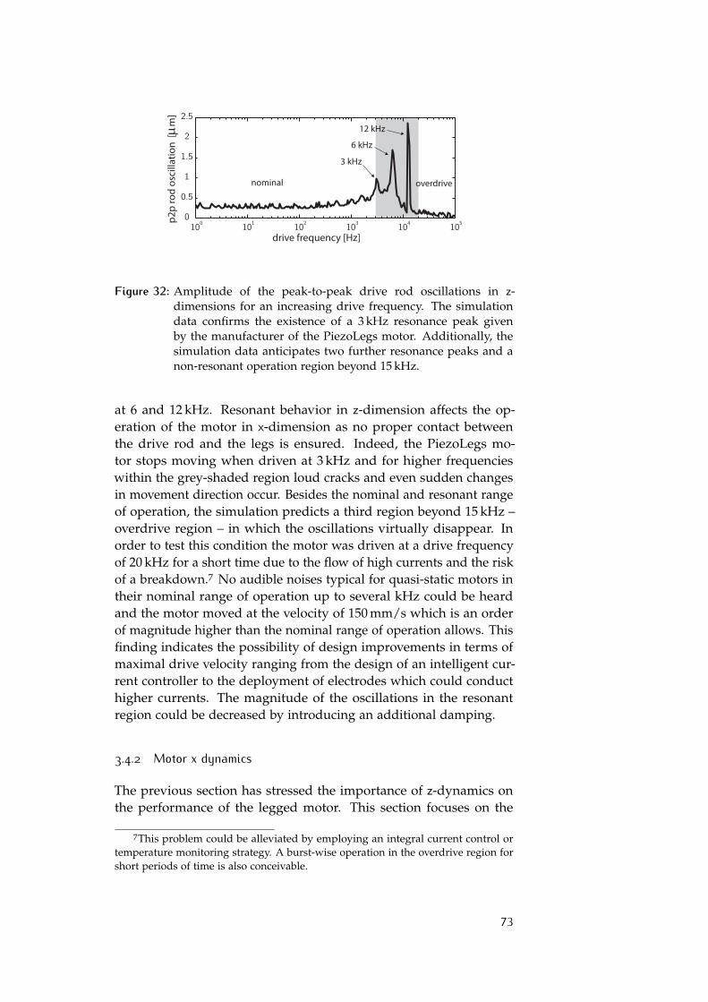


![2016 Siviy (Dynamic Walking) POSTER - Optimization of soft ... · [7] Lee et al., ICRA, 2016. Title Microsoft PowerPoint - 2016 Siviy (Dynamic Walking) POSTER - Optimization of soft](https://static.documents.pub/doc/80x56/5ed78b18ec73a923ab52da7a/2016-siviy-dynamic-walking-poster-optimization-of-soft-7-lee-et-al-icra.jpg)


