Dynamic Modeling and Control of a Crystallization Process ...

Dynamic Modeling and Control of a

Crystallization Process Using Neural

Networks

Gabriel Fiúza M. de Miranda

Final Project Report

SupervisorsMaurício Bezerra de Souza Jr., D. Sc.

Bruno Didier Olivier Capron, D.Sc.

Marcellus G. F. de Moraes, M. Sc.

June 2021

Dynamic Modeling and Control of a Crystallization

Process Using Neural Networks

Gabriel Fiúza Moreira de Miranda

Final project report in chemical engineering submitted to the faculty of the

School of Chemistry (EQ/UFRJ) as part of the requirements for obtaining

the degree of Chemical Engineer.

Approved by:

(Argimiro Resende Secchi, D.Sc.)

(Amaro Gomes Barreto Jr., D.Sc.)

Supervised by:

(Maurício Bezerra de Souza Jr., D.Sc)

(Bruno Didier Olivier Capron, D.Sc.)

(Marcellus G. F. de Moraes, M.Sc.)

Rio de Janeiro, RJ - Brazil

June 2021

i

Miranda, Gabriel Fiúza M. de

Dynamic Modeling and Control of a Crystallization Process Using Neural

Networks/Gabriel Fiúza M. de Miranda - Rio de Janeiro: UFRJ/EQ, 2021

XIII, 101 p.; il.

(Final Project Report) - Universidade Federal do Rio de Janeiro, Escola

de Química, 2021.

Supervisors: Maurício Bezerra de Souza Jr., Bruno Didier Olivier Capron,

Marcellus G. F. de Moraes

1. Crystallization processes. 2. Neural Networks. 3. Population Balance.

4. Process Control.

ii

Acknowledgments

First of all, I would like to thank my parents for providing unconditional

love and support throughout not only these university years, but every single

second since I first put my feet on this earth. For this I am deeply grateful.

Secondly, I would like to thank my sister for being my full-time partner in

crime and for sharing with me most of the experiences that have contributed

to shaping the person I am today. Even when we are physically far from each

other she manages to reassure me that distance is just a number, and that

she is right here with me even when we are kilometers apart.

I would also like to thank the many friends I made during these years

at UFRJ. I can not imagine going through this long and tiring (although

rewarding) process without their help to take the edge off and make the road

a bit lighter and a lot funnier.

I thank the many friends I made during my exchange years in France and

that I, without a doubt, will keep for the remainder of my life. The whole

process of living abroad, learning a new language and attending a high level

international institution was certainly challenging, and I am glad to have had

each one of them by my side.

Lastly, I thank my supervisors for the continuous support and the relevant

discussions throughout the development of this project.

iii

Agradecimentos

Em primeiro lugar, eu gostaria de agradecer aos meus pais pelo amor e

suporte incondicionais ao longo não só desses anos de universidade, mas

de cada segundo da minha vida. Por terem me proporcionado todos os

meios possíveis e imagináveis para me dedicar aos estudos enquanto eles

se ocupavam de todo o resto. Parece clichê, mas precisa ser dito: sem eles

nada disso seria possível, e por isso eu sou profundamente grato.

Em segundo lugar, eu gostaria de agradecer à minha irmã por ser minha

maior parceira e por ter compartilhado comigo muitas das experiências que

contribuíram para formar quem eu sou hoje. Mesmo quando estamos dis-

tantes fisicamente ela encontra maneiras de se fazer presente e me mostrar

que a distância é apenas um número, e que ela está sempre comigo não

importa quantos kilômetros haja entre nós.

Também gostaria de agradecer aos muitos amigos que fiz ao longo desses

anos na UFRJ. Eu realmente não consigo imaginar passar por esse processo

longo e cansativo (apesar de muito gratificante) sem a ajuda deles para tornar

a caminhada um pouco mais leve e muito mais divertida.

Agradeço aos muitos amigos que fiz durante os anos de intercâmbio na

França e que, sem a menor dúvida, levarei comigo pro restante dessa vida.

Todo o processo de viver fora do país, aprender uma nova língua e frequentar

uma instituição de ensino de alta qualidade foram bem desafiadores, e eu sou

muito grato por ter tido a companhia de cada um deles ao longo disso tudo.

Por fim eu agradeço aos meus orientadores por todo o suporte e discussões

relevantes ao longo do desenvolvimento desse projeto.

iv

Abstract of the Final Project Report presented to the School of Chemistry

as part of the requirements for obtaining the degree of Chemical Engineer.

Dynamic Modeling and Control of a CrystallizationProcess Using Neural Networks


June, 2021

Supervisors: Prof. Maurício Bezerra de Souza Jr., D.Sc

Prof. Bruno Didier Olivier Capron, D.Sc.

Prof. Marcellus G. F. de Moraes, M.Sc.

In industrial crystallization processes, the control of the size and shape of

the crystals is of considerable relevance. In this work, we use experimental

data to develop neural network models of the batch crystallization of potas-

sium sulfate (K2SO4). First, a dynamic model of the system capable of pre-

dicting its state in the near future with good accuracy given its present and

past states is developed. Secondly, an inverse model of the process capable

of calculating the control moves to be implemented for the system to follow a

desired reference trajectory is developed. Last, this controller’s performance

is investigated by simulating a closed-loop control scheme in which a popula-

tion balance model is used to represent the real process plant. We show that

the choice of reference trajectory has a strong influence on the controller’s

performance in terms of batch duration, the error between the system state

and the set-point, and required control effort. The best trajectory presented

results that were 70% to 140% better than the other trajectories in terms of

the above criteria.

v

Resumo do Projeto Final apresentado à Escola de Química como um dos

requisitos para a obtenção do título de Engenheiro Químico.

Modelagem Dinâmica e Controle de um Processo deCristalização Utilizando Redes Neuronais


Junho, 2021

Supervisors: Prof. Maurício Bezerra de Souza Jr., D.Sc

Prof. Bruno Didier Olivier Capron, D.Sc.

Prof. Marcellus G. F. de Moraes, M.Sc.

Nos processos industriais de cristalização, o controle do tamanho e da

forma dos cristais é de considerável importância. Nesse trabalho, dados

experimentais são utilizados para desenvolver modelos de redes neuronais

para o processo de cristalização em batelada do sulfato de potássio (K2SO4).

Primeiramente, um modelo dinâmico do sistema capaz de prever seu estado

em um futuro próximo dadas as suas condições atuais é desenvolvido. Em

seguida, um modelo inverso do processo capaz de calcular a próxima ação

de controle a ser implementada para conduzir o sistema a uma trajetória

de referência é desenvolvido. Finalmente, o desempenho desse controlador é

investigado através da simulação de uma malha fechada em que um modelo

de balanço populacional é utilizado como processo real. Nós mostramos que

a escolha da trajetória de referência tem forte influência sobre o tempo de

duração da batelada, erro final entre estado do sistema e set-point e esforço

de controle. Em termos dos critérios acima, a melhor trajetória apresentou

resultados de 70% a 140% melhores que as demais.

vi

Contents

List of Tables x

List of Figures xi

1 Introduction 1

1.1 Motivation . . . . . . . . . . . . . . . . . . . . . . . . . . . . . 1

1.2 Objectives . . . . . . . . . . . . . . . . . . . . . . . . . . . . . 2

1.3 Text Outline . . . . . . . . . . . . . . . . . . . . . . . . . . . . 3

2 Bibliography Review 5

2.1 Machine Learning and Neural Networks . . . . . . . . . . . . . 5

2.2 Multilayer Perceptron NN’s . . . . . . . . . . . . . . . . . . . 7

2.2.1 Training MLP NN’s . . . . . . . . . . . . . . . . . . . . 11

2.2.2 Overfitting . . . . . . . . . . . . . . . . . . . . . . . . . 15

2.2.3 Model Assessment . . . . . . . . . . . . . . . . . . . . 18

vii

2.3 Applications of NN’s in Chemical Engineering . . . . . . . . . 20

2.3.1 Process Identification . . . . . . . . . . . . . . . . . . . 20

2.3.2 Process Control . . . . . . . . . . . . . . . . . . . . . . 22

2.4 Crystallization Processes . . . . . . . . . . . . . . . . . . . . . 28

2.4.1 Crystallization Mechanisms . . . . . . . . . . . . . . . 30

2.4.2 Particle Size Distribution . . . . . . . . . . . . . . . . . 34

2.5 Data-Driven Modeling of Crystallization Processes: Related

Works . . . . . . . . . . . . . . . . . . . . . . . . . . . . . . . 36

3 Methodology 39

3.1 Experimental Setup . . . . . . . . . . . . . . . . . . . . . . . . 39

3.2 K2SO4 Crystallization . . . . . . . . . . . . . . . . . . . . . . 41

4 Direct MLP Model 43

4.1 Exploratory Data Analysis and Preprocessing . . . . . . . . . 44

4.2 Baseline Direct Model . . . . . . . . . . . . . . . . . . . . . . 50

4.3 Model Evaluation . . . . . . . . . . . . . . . . . . . . . . . . . 52

4.4 Sensitivity to Past Inputs . . . . . . . . . . . . . . . . . . . . 55

4.5 Improving the Direct MLP Model: Hyperparameter Tuning . . 56

5 Inverse MLP Model 65

5.1 Baseline Inverse Model . . . . . . . . . . . . . . . . . . . . . . 66

viii

5.2 Model Evaluation . . . . . . . . . . . . . . . . . . . . . . . . . 67

5.3 Improving the Inverse Model: Hyperparameter Tuning . . . . 69

6 Closed Loop Control 72

6.1 Description of the PB Model for K2SO4 Crystallization . . . . 72

6.1.1 Simulation of the PB Model . . . . . . . . . . . . . . . 75

6.2 Control Loop . . . . . . . . . . . . . . . . . . . . . . . . . . . 77

6.2.1 Defining a Reference Trajectory . . . . . . . . . . . . . 78

6.2.2 Comparison of Different Reference Trajectories . . . . . 86

7 Conclusions 89

7.1 Future Work . . . . . . . . . . . . . . . . . . . . . . . . . . . . 91

ix

List of Tables

4.1 CV MSE for the 5 models considered. . . . . . . . . . . . . . . 56

4.2 CV MSE for the 5 models optimized with Optuna. . . . . . . 58

5.1 CV MSE for the 4 inverse models optimized with Optuna. . . 70

6.1 Values for each of the criteria and cost for each reference tra-

jectory. . . . . . . . . . . . . . . . . . . . . . . . . . . . . . . . 87

x

List of Figures

2.1 Basic structure of an MLP network. . . . . . . . . . . . . . . . 9

2.2 A neuron with 5 inputs. . . . . . . . . . . . . . . . . . . . . . 9

2.3 Common activation functions in neurons. . . . . . . . . . . . . 11

2.4 Test and training error as a function of model complexity [3]. . 16

2.5 Examples of low, high and intermediate complexity models. . . 17

2.6 K-fold cross validation split. Adapted from [3] . . . . . . . . . 19

2.7 Series-parallel or parallel identification methods. [16] . . . . . 22

2.8 MPC scheme. . . . . . . . . . . . . . . . . . . . . . . . . . . . 23

2.9 NN as the controller. Adapted from [26] . . . . . . . . . . . . 26

2.10 NN as the controller scheme. [26] . . . . . . . . . . . . . . . . 27

2.11 Solubility and metastability diagram [33]. . . . . . . . . . . . . 29

2.12 Crystallization mechanisms. Adapted from [34]. . . . . . . . . 30

2.13 Critical Gibbs free energy change as a function of cluster ra-

dius. Adapted from [34]. . . . . . . . . . . . . . . . . . . . . . 32

xi

3.1 Experimental setup. . . . . . . . . . . . . . . . . . . . . . . . 40

4.1 Result of applying moving average to a given experiment. . . . 45

4.2 Histograms of the complete dataset. . . . . . . . . . . . . . . . 46

4.3 Data distributions for 3 different scenarios. . . . . . . . . . . . 49

4.4 Lag correlation analysis. . . . . . . . . . . . . . . . . . . . . . 50

4.5 Baseline NN architecture. . . . . . . . . . . . . . . . . . . . . 51

4.6 10-Fold Cross-Validation to determine preprocessing strategy. 53

4.7 Evaluation of Model 1 - Training. . . . . . . . . . . . . . . . . 53

4.8 Evaluation of Model 1 - Test. . . . . . . . . . . . . . . . . . . 54

4.9 Model sensitivity to past inputs. . . . . . . . . . . . . . . . . . 56

4.10 CV MSE for the 5 models optimized with Optuna. . . . . . . 58

4.11 Evaluation of the Optimized Model 3 - Training. . . . . . . . . 59

4.12 Evaluation of the Optimized Model 3 - Test. . . . . . . . . . . 60

4.13 Evaluation of the Optimized Model - Complete experiment (1). 61

4.14 Evaluation of the Optimized Model - Complete experiment (2). 62

4.15 Long-term predictions. Looping Optuna’s best model (1). . . . 63

4.16 Long-term predictions. Looping Optuna’s best model (2). . . . 64

5.1 Baseline inverse model architecture. . . . . . . . . . . . . . . . 66

5.2 Evaluation of the baseline inverse model. . . . . . . . . . . . . 68

xii

5.3 Evaluation of the baseline inverse model - Complete experiments. 68

5.4 CV MSE for the 4 inverse models optimized with Optuna. . . 70

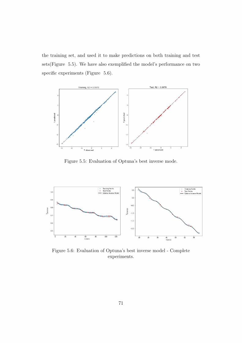
5.5 Evaluation of Optuna’s best inverse mode. . . . . . . . . . . . 71

5.6 Evaluation of Optuna’s best inverse model - Complete exper-

iments. . . . . . . . . . . . . . . . . . . . . . . . . . . . . . . . 71

6.1 Simulation of the PB model and comparison to experimental

results for a constant temperature profile. . . . . . . . . . . . . 75

6.2 Simulation of the PB model and comparison to experimental

results for a varying temperature profile. . . . . . . . . . . . . 76

6.3 Proposed scheme for the control loop. . . . . . . . . . . . . . . 77

6.4 Simulation of the control loop for a constant reference trajectory. 79

6.5 Simulation of the control loop for a reference trajectory defined

by 1st order dynamics. . . . . . . . . . . . . . . . . . . . . . . 80

6.6 Defining a 2nd order reference trajectory for each of the mo-

ments. . . . . . . . . . . . . . . . . . . . . . . . . . . . . . . . 82

6.7 Simulation of the control loop for a reference trajectory defined

by 2nd order dynamics. . . . . . . . . . . . . . . . . . . . . . . 83

6.8 Simulation of the control loop for an adaptive 1st order refer-

ence trajectory. . . . . . . . . . . . . . . . . . . . . . . . . . . 85

6.9 Evolution of the error ε and the control effort ce for each ref-

erence trajectory. . . . . . . . . . . . . . . . . . . . . . . . . . 87

xiii

Chapter 1

Introduction

1.1 Motivation

Crystallization is a chemical process that finds widespread application in

industrial units as a solid-fluid separation technique. It is known to produce

high purity products on a single and relatively simple equipment, which

makes it specially attractive for the production of solid materials [1]. In

industry, crystallization is usually followed by other unit operations such as

filtering and drying. In these processes, the size and shape of the crystals

are of considerable importance. They determine the operating conditions of

these equipments and directly influence the properties of the final product.

Attaining product specification and production yields requires knowledge

about the underlying processes and their sensitivity to different operating pa-

rameters. Modeling these processes can bring valuable information on how

to conduct and control them to meet the desired criteria. However, crystal-

lization processes present highly nonlinear behavior, requiring sophisticated

1

modeling frameworks such as population balances (PB) [2]. These models

usually contain multiple parameters that have to be estimated from exper-

imental data, a task that might prove difficult due to the wide variety of

existing crystallization setups and operating conditions.

In this sense, machine learning (ML) algorithms, and neural networks

(NN) in particular, provide an alternative modeling framework that is uni-

versal and highly flexible. If enough data about the inputs and outputs to

the process is available, a ML model can be trained to identify patterns

in these input-output pairs without making simplifying assumptions about

which mechanisms are in play.

1.2 Objectives

In this project, we wish to investigate the suitability of using NN’s for

the dynamic modeling and control of the batch crystallization of potassium

sulfate (K2SO4). This inorganic salt was chosen as a first step towards devel-

oping models for more complex substances because it is cheap and well suited

to the process monitoring techniques adopted in this work (image analysis).

We aim to accomplish this by using real experimental data regarding the size

and shape distribution of these crystals to develop two different models - one

for the system’s dynamic behavior, and one that can be used to control this

dynamic behavior. This controller will then be tested on a simulated process

plant which is described by a population balance with estimated parameters.

With this simulation, the objectives are assessing the controller’s ability to

make the system follow a reference trajectory, defined in terms of crystal

size and shape, and providing insight on how to operate batch crystallization

2

units in order to achieve higher yields, shorter operating times, and lower

energy consumption.

1.3 Text Outline

The text is organized as follows:

Chapter 2 contains the bibliography review - section 2.1 presents general

concepts regarding ML; in section 2.2 we cover the basic structure, math-

ematical aspects and training methods of classical NN’s; in section 2.3 we

present a few applications of NN’s in chemical engineering; in section 2.4 we

review some of the literature on crystallization processes and in section 2.5

we present related works concerning data-driven dynamic models of crystal-

lization processes.

Chapter 3 describes the experimental methods relevant to this project.

The experimental setup for the batch crystallization of K2SO4 is presented.

Chapter 4 concerns the development of a direct NN model of the crys-

tallization process, which can predict the state of the system over a short

horizon given its present and past states.

Chapter 5 concerns the development of an inverse NN model of the

process, which acts as a controller of the crystallization process, calculating

the next control move to be implemented in order for the system to follow a

reference trajectory.

Chapter 6 contains the simulation of a control loop in which the process is

modeled by a population balance and the controller is the inverse NN model

3

developed in Chapter 5.

Chapter 7 briefly discusses the results and suggests further developments.

4

Chapter 2

Bibliography Review

2.1 Machine Learning and Neural Networks

Machine learning is the process of deriving mathematical models that can

learn from data. In a typical scenario, we have outcome data - that could be

quantitative (such as stock prices) or categorical (such as a patient having

diabetes or not) - that we wish to predict based on a series of features or

predictors. To do so, we use the available data on outcomes and features

to train a model that we hope will be capable of predicting outcomes on

unseen data when presented with it. A good model is one that is capable of

generalizing well the rules learned during training - it can learn the underlying

structure and relationships of the training data without loosing generalization

power [3].

ML problems are typically classified into three main groups according to

5

the data used to develop them: supervised, unsupervised and reinforcement

learning. When training a supervised model, we need labeled data: for a

given instance or sample, we need to know the right answer to that predic-

tion problem. Imagine our example of the patient with diabetes: to train a

supervised learning model that is capable of predicting if a new patient has

diabetes or not based on their blood work, each sample in our dataset should

consist of a series of features used as predictors and of a target class - the

right answer to that specific prediction problem. In contrast, unsupervised

learning models are trained on datasets that consist solely of features and

have no outcome measurements. In these types of problems, we are interested

in describing how the data is organized or clustered. The most common ap-

plication of unsupervised learning is clustering: imagine you are the owner of

a music streaming service and you wish to recommend new music to a given

user. One way of doing so is by trying to cluster users into groups with some-

thing in common, and then recommending to a given user what some of his

cluster colleagues are listening to. In the third main group, reinforcement

learning, the goal is to determine how intelligent agents should act in or-

der to maximize a function that represents a cumulative reward. This agent

learns by trial and error through interactions with a dynamic environment

[3, 4].

In the supervised scenario, which is the main interest of this work, prob-

lems are further classified into two groups: regression and classification. In

regression problems, our objective is to predict the value of a continuous vari-

able - such as the stock price example above; while, in classification problems,

we are interested in determining which of a series of categorical classes best

describes a given data sample - e.g., based on a patient’s blood work we wish

to determine if they have diabetes or not, or based on the contents of an

6

e-mail we wish to determine if it is a spam or not.

ML and artificial intelligence (AI) are broad fields with a lot of recent

advances. There are numerous ML models from which to choose today, each

one being most adapted to a certain problem or dataset. In this project, we

are mainly interested in one class of models called Neural Networks (NN),

which will be covered in more detail in the following sections. However, some

of the concepts related to developing NN models are universal and can be

applied to other classes of ML models.

2.2 Multilayer Perceptron NN’s

Before proceeding with the foundations of how NN’s work, let us fix some

notation to be used throughout this work. We will denote scalar variables by

lower-case letters (x) and vectors by lower-case boldface letters (x). We take

all vectors to be column vectors, and we obtain row vectors by transposing

them (xT ). Matrices are denoted by upper-case boldface letters (X).

NN’s are part of a class of models called deep learning models, and the

most basic model of this class is the feedforward neural network, or multi-

layer perceptron (MLP). An MLP is just a mathematical function f map-

ping a set of input values x (or features) to output values y (or outcomes).

The function is formed by a combination of much simpler functions in a sort

of modular architecture. These models are called feedforward because the

information in the network flows from an initial set of features x into the

intermediate computations that define the function f mapping, and finally

to the output y. They do not exhibit feedback connections in which model

outputs or intermediate outputs are fed back into themselves. When we ex-

7

tend MLP networks with feedback connections we create recurrent neural

networks such as the LSTM [5] and GRU architectures [6, 7].

The architecture of a NN is based on the physiology of the neural sys-

tems of animals and humans, in which multiple neurons are interconnected

through synapses. In artificial NN’s, artificial neurons are arranged in layers

called input, hidden, and output layers. The number of hidden layers and

neurons are hyperparameters of the network. They receive this name since

they are not optimized during training, and the person developing the model

should rely on other techniques to tune them. The structure of the input and

output layers, on the other hand, is fixed according to the structure of the

prediction problem. The neurons in the input layer receive the inputs or fea-

tures, while neurons in the output layer predict the outputs of the variables

we are interested in. The hidden layers that connect input to output are the

ones responsible for learning the patterns in the training data. Figure 2.1

presents the general structure of an MLP network [7].

The basic computing unit in a NN is called a neuron and is represented

by the nodes in Figure 2.1. A neuron is a mathematical model that receives

multiple inputs and produces a single scalar output. In Figure 2.2, each

input xi is multiplied by a synaptic weight wi. These weights are adjustable

(or trainable) parameters in the network, meaning the network learns by

adjusting the values of the weights that connect different neurons. Indicated

by b is the bias associated with the neuron, another one of the trainable

parameters [7].

8

Figure 2.1: Basic structure of an MLP network.

Figure 2.2: A neuron with 5 inputs.

Inputs, synaptic weights and bias are combined in a specific way and fed

9

to an activation function, which provides the output y. Let us denote the

neuron’s activation function by g(h). The output y is thus given by:

h =m∑i=1

xiwi + b (2.1)

y = g(h) (2.2)

There are multiple possible choices for the activation function used in the

hidden layers, and this choice is yet another one of the hyperparameters of the

network. Neurons in the input layer generally do not present an activation

function - their task is to simply pass the initial features forward. The choice

of the activation function in the output layer is generally conditioned by the

type of data we wish to predict. In regression problems, where we try to

predict real valued variables, the activation function in the output layer is

generally a linear function. If, however, we are trying to predict a binary

class (yes or no), we could use the sigmoid or logistic function, while the

softmax function is indicated for multiclass prediction [7]. Shown in Figure

2.3 are a few of the most common functions used as activation functions.

10

Figure 2.3: Common activation functions in neurons.

2.2.1 Training MLP NN’s

The task of training a NN is basically an optimization problem that aims

at finding the values of the weights wi and biases b such that the output

of the network y(x) is close enough to the correct outcomes y(x) for all n

samples x in the training dataset. To quantify how well the network is doing

on this prediction task, we define a cost function (or objective function)

to be optimized. There are multiple cost functions available that should be

chosen according to the problem at hand. We will only address one of the

most straightforward cost functions used for regression problems: the Mean

Squared Error (MSE) cost function (equation 2.3) [7]:

J(W ) =1

2n

∑x

||y(x)− y(x)||2 (2.3)

11

For simplicity, we represent by W the matrix of weights w and biases b

associated with the complete network (although, rigorously, there would be

one matrix W l associated with each pair of layers in the network, where l

denotes the layer that receives the inputs). In our notation, J(W ) is, then,

the scalar cost associated with the set of parameters W . This cost function

should look familiar, as it is used in classic regression algorithms such as Least

Squares. By inspection, we notice that J(W ) in non-negative, and that its

value becomes smaller as the outputs of the network y(x) are approximately

equal to the correct outcomes y(x). The aim of the training algorithm is

to use the training data to gradually update the values of W in order to

minimize the value of the cost function [8].

The training process is nothing more than an optimization problem, and

one of the most widely used algorithms is the Gradient Descent algorithm [9].

This basic algorithm has suffered numerous modifications and improvements

over the years, but it is still the starting point in understanding how NN’s

learn. In deep learning, the gradient descent is also called the backpropa-

gation algorithm [10].

When we use an MLP network to process an input x and produce an out-

put y, information flows through the network in a forward direction. This

is called forward propagation. During training, forward propagation con-

tinues until it produces a scalar cost J(W ). The backpropagation algorithm

allows information from the cost to then flow backward through the network

in order to compute the gradient with respect to parameters W [7].

The gradient of J(W ) indicates in which direction of the space defined

by the entries in W the cost J increases the most. If we want to decrease

J , we should move in the direction opposite to the gradient. The general

12

process proceeds as following: we compute the gradient of the cost function

with respect to W for every one of the n samples in the training set and then

calculate the average gradient. Weights are then iteratively updated in the

direction opposite to the average gradient. Equation 2.4 shows how weights

at a given iteration are updated from their values at the preceding iteration,

the average gradient across all samples and a parameter λ called learning

rate:

W ∗ = W − λ∂J(W )

∂W(2.4)

Parameter λ is called the learning rate as it dictates how big of a step we

take in the direction of minimizing the cost. A small value of λ will result

in a slow optimization process, but might be more numerically stable. Too

large of a value may cause the algorithm to diverge.

In practice, calculating the average gradient across all samples is too time

consuming, and a subset (batch) of the training set is used to compute the

gradient at each iteration. This modification is called the Batch Gradient

Descent or Stochastic Gradient Descent [11, 12]. Other variations on the clas-

sic backpropagation algorithm are the Momentum and Adam optimization

procedures [10, 13].

The Adam optimization procedure, which will be used in this work,

incorporates the idea of momentum. The algorithm calculates exponential

moving averages of the gradient and the squared gradient, where two ad-

ditional hyperparameters control the decay rates of these moving averages.

The moving averages are estimated from the 1st moment (mean) and 2nd raw

moment (uncentered variance) of the gradient. In Adam’s update rule (given

13

by a different, but equivalent equation to equation 2.4), there are different

learning rates associated with each of the predictors, and these learning rates

get automatically updated as training proceeds [13].

A full derivation of the backpropagation algorithm or its variations is out

of the scope of this project, but the reader can refer to [14] or many other

available sources. In short, the chain rule of differentiation is applied to

equation 2.3 to calculate the gradient of the cost function with respect to each

trainable parameter inW . This is achieved by decomposing the cost function

into simpler functions representing the intermediate calculations performed

by the network and moving backwards (backpropagating the errors) along

the network. Equation 2.4 will thus present different expressions depending

on the position of the neurons on the network and on the choice of activation

functions.

One final remark concerning the training of NN models is feature scaling.

As with many other ML algorithms (such as Ridge and Lasso regression, K-

Nearest Neighbors, Principal Component Analysis, etc.), features should be

scaled before being fed to NN’s [3]. This need arises since the scaling of the

inputs determines the scaling of the weights connecting the input layer to the

first hidden layer. As we have seen in figure 2.3, most activation functions

used in neurons are active when the activation signal is close to zero. It is

thus common practice to scale inputs so that each feature has either zero

mean and unit variance or vary between zero and unity. This also has the

effect of bringing all variables, which may vary over very different ranges, to

the same variation range.

Two of the most common scaling techniques are min-max scaling and

standardization:

14

z =x−min(x)

max(x)−min(x)(2.5)

z =x− x

σ(2.6)

where min(x) and max(x) are the minimum and maximum values of

feature x in the training data, x is the mean of input x across all samples

in the training data, and σ its standard deviation.

Note that the exact same scaling has to be applied to training and test

sets. The quantities min(x), max(x), x and σ are calculated on the training

data and the resulting scaling is applied to training and test sets.

2.2.2 Overfitting

We have been talking about a training dataset but have not yet defined

it. Most ML algorithms divide the available dataset into a training and a

test set (and additionally a validation set, explained further below), which

serve different purposes. The training set is used by the backpropagation

algorithm in order for the network to learn the optimal values of the trainable

parameters. The test set, on the other hand, is not presented to the network

during training, and is used after training has finished to assess the model’s

generalization power. A common split into training and test sets is to use

70% of the data for training and the remaining 30% for testing [3].

Often neural networks have too many weights and will overfit the training

data even if the global minimum of the cost function is reached. We say

a network is overfitting the training data if it produces predictions more

15

accurately in the training set than in the test set. This concept is based

on a more general aspect of statistical models called Bias-Variance Tradeoff,

which is illustrated by Figure 2.4 [3].

Low complexity models such as a linear regression will typically present

errors due to the model being biased. High complexity models with lots of

parameters will present low bias but high variance. Models to the left of

Figure 2.4 are said to be underfitted, while models on the right are said

to be overfitted. There is some intermediate complexity at which the model

performs best in terms of generalization power. This is further exemplified

in figure 2.5.

Figure 2.4: Test and training error as a function of model complexity [3].

In this project we have used the Early Stopping and Regularization tech-

niques to reduce overfitting. Early Stopping interrupts the training process

before reaching the minimum of the cost function. This is usually done by

monitoring the value of the prediction error in a test (or validation) set

16

Figure 2.5: Examples of low, high and intermediate complexity models.

along the training epochs and stopping training if no significant reduction

in the cost is observed. Regularization reduces overfitting by introducing

a penalty term into the cost function defined in equation 2.3. There are

different forms of regularization available, that vary on the type of penalty

imposed on the cost. The most common ones are the L1 and L2 Regular-

ization, whose expressions are respectively shown [3]:

J(W ) =1

2n

∑x

||y(x)− y(x)||2 + α||W || (2.7)

J(W ) =1

2n

∑x

||y(x)− y(x)||2 + α||W ||2 (2.8)

These expressions help reducing overfitting by imposing a penalty on the

size of the weights in the network. A network with smaller weights should,

17

intuitively, be less prone to taking some of the patterns in the training data

to be considerably more important than others. [15]

Other aspects that help control overfitting are the number of hidden layers

and of hidden neurons. These parameters, along with the choice of activation

functions, the penalty term α in equations 2.7 and 2.8 and the learning rate

λ in equation 2.4 are said to be hyperparameters of the network. The combi-

nation of hyperparameters that produces best prediction results depends on

the problem at hand, the quality and the quantity of data. Small datasets,

for example, do not carry enough information to be able to train complex

deep neural networks.

2.2.3 Model Assessment

Ideally, if we had enough data, we would simply assess our model’s perfor-

mance and generalization capacity by evaluating its predictions on a test set

which it had not seen before. When dealing with small datasets, however,

this may prove difficult. Splitting the initial dataset into training and test

sets is done randomly, and often the resulting split has a strong influence

on the performance of the model. This characteristic makes it difficult, for

example, to compare different models: one model may perform best when

data is split in a given way, while another model would perform best if the

split had been different [3].

One simple way of overcoming this difficulty is throughCross-Validation

(CV). K-fold CV splits the complete dataset into K equal-sized parts. If K

= 5, the picture looks like Figure 2.6 [3].

For the kth part (in red), we fit the model to the other K-1 parts of the

18

Figure 2.6: K-fold cross validation split. Adapted from [3]

data, and use the kth as a test set (in this context called a validation set) to

assess the model’s prediction error. We do this for k = 1, 2, . . . ,K and

average the K estimates of the prediction error. In this way, every sample

in the dataset is eventually part of the test set, and we get a more robust

estimate of the model’s generalization power [3].

The concept of a validation set also arises when tuning the hyperparam-

eters of the network. Let’s say we have trained 5 different NN models with

different hyperparameters for each. To determine which set of hyperparam-

eters is the best, common practice is to take the complete dataset and split

it into training, validation, and test sets (a typical split would be 70:10:20).

The validation set, in this context, is used after training to select the best

among candidate models. If we adjust the hyperparameters based on their

performance on the test set, we might be selecting hyperparameters that

perform best on this particular split. The test set should only be used

for final model evaluation. Alternatively, a K-fold CV procedure can be

performed to choose from candidate models [3].

19

2.3 Applications of NN’s in Chemical Engineer-

ing

A number of applications of NN’s in chemical engineering have been reported,

in the dynamic modeling and control of chemical processes, but also in

fault diagnosis, soft sensors, data reconciliation, etc. [16, 17]. Process plants

are usually complex and unique - the different plant sizes, feedstocks, ages,

piping, etc. make it difficult to use first principles modeling approaches to

each specific situation. NN’s have the advantage of being flexible, easy to

apply and efficient in using process data for modeling [18].

This current project focuses on the use of NN’s for process identification

and control, and thus the topic will be covered in more detail in sections

2.3.1 and 2.3.2.

2.3.1 Process Identification

Given some discrete data relating process inputs and outputs, nonlinear pro-

cesses can be modeled by the following generalized equation [16]:

y(k+ 1) =f1[y(k),y(k− 1), ...,y(k− n+ 1)]

+ g1[u(k),u(k− 1), ...,u(k−m+ 1)](2.9)

Where u(k) and y(k) denote, respectively, model inputs and outputs

at time instant k; m and n are the process orders, and f and g are some

arbitrary nonlinear functions that we wish to estimate. When identifying

such a model using a NN, the relationship between the inputs (y(k), y(k−

20

1), ..., y(k−n+1)); (u(k), u(k−1), ..., u(k−m+1)) and the network

output y(k+ 1) is given by [16]:

y(k+ 1) =f1[y(k),y(k− 1), ...,y(k− n+ 1)]

+ g1[u(k),u(k− 1), ...,u(k−m+ 1)](2.10)

In this method, the weights of the network are updated during training by

comparing the predicted outputs with the real outputs observed on process

data. The above approach for estimating the parameters of the dynamic

model is called "series-parallel" identification [16, 18]. Another identification

method is called "parallel" identification, in which the outputs from the

network are fed back to itself forming a loop. In this case, the model equation

can be written as:

y(k+ 1) =f1[y(k), y(k− 1), ..., y(k− n+ 1)]

+ g1[u(k),u(k− 1), ...,u(k−m+ 1)](2.11)

Figure 2.7 illustrates these different approaches [16]. In the case where

the pivot connects to "msp", the plant output is directly fed to the model

for prediction during training. In comparison, when the pivot is connected

to "mp", the plant output is not fed to the model. In the latter case, the

model is completely in parallel with the plant.

Based on equation 2.10, the "series-parallel" configuration can be seen as

a one-step ahead modeling approach. At each time instant, current process

data is used to estimate the state of the process one time-step into the future.

In contrast, equation 2.11 suggests the use of the "parallel" configuration for

long-range predictions. Model outputs become model inputs at a later time-

21

step, and we can look into the future as far as we wish by proceeding with

this looping procedure. It should be noted that this might lead to numerical

instability if the initial model is not sufficiently accurate [18].

Figure 2.7: Series-parallel or parallel identification methods. [16]

2.3.2 Process Control

Multiple applications of NN’s for process control have been reported. One

of the most common applications involves nonlinear model predictive control

22

(NMPC) [19–21]. Other authors have succesfully applied NN’s to detect pro-

cess faults [22, 23], correct sensor erros [24] and for tracking batch processes

[25].

In predictive controllers based on process models, the model is used to

predict future outputs from the system, and an optimization procedure is

carried out to calculate the optimal future control actions that minimize the

error between a reference trajectory (or set-point) and these output predic-

tions [18]. Figure 2.8 exemplifies this procedure.

Figure 2.8: MPC scheme.

In Figure 2.8, the process model (which can be given by a NN) is used to

predict the future process outputs. The control actions to be implemented

in the future are such that the predicted process outputs track the refer-

ence trajectory over a given prediction horizon of p samples. MPC can be

formulated as an optimization problem, in which we want to minimize an

objective function by choosing values of the manipulated variable in the fu-

23

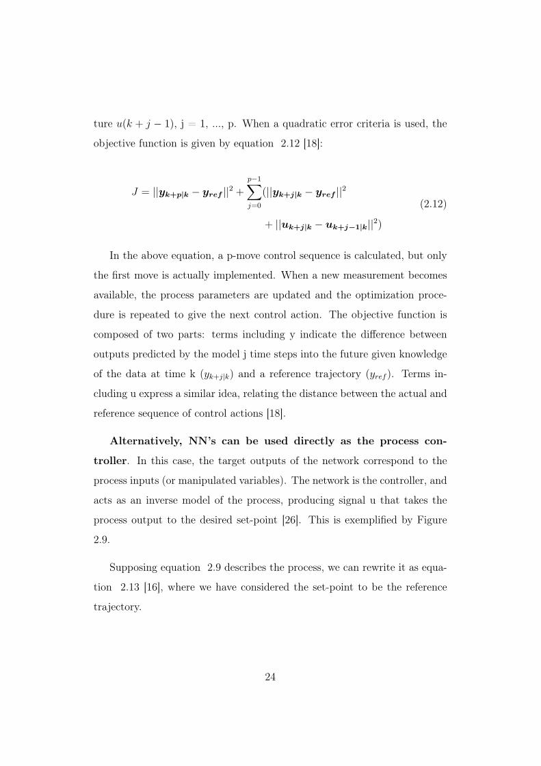
ture u(k + j − 1), j = 1, ..., p. When a quadratic error criteria is used, the

objective function is given by equation 2.12 [18]:

J = ||yk+p|k − yref ||2 +

p−1∑j=0

(||yk+j|k − yref ||2

+ ||uk+j|k − uk+j−1|k||2)

(2.12)

In the above equation, a p-move control sequence is calculated, but only

the first move is actually implemented. When a new measurement becomes

available, the process parameters are updated and the optimization proce-

dure is repeated to give the next control action. The objective function is

composed of two parts: terms including y indicate the difference between

outputs predicted by the model j time steps into the future given knowledge

of the data at time k (yk+j|k) and a reference trajectory (yref ). Terms in-

cluding u express a similar idea, relating the distance between the actual and

reference sequence of control actions [18].

Alternatively, NN’s can be used directly as the process con-

troller. In this case, the target outputs of the network correspond to the

process inputs (or manipulated variables). The network is the controller, and

acts as an inverse model of the process, producing signal u that takes the

process output to the desired set-point [26]. This is exemplified by Figure

2.9.

Supposing equation 2.9 describes the process, we can rewrite it as equa-

tion 2.13 [16], where we have considered the set-point to be the reference

trajectory.

24

u(k) =f−12 [sp,y(k),y(k− 1), ...,y(k− n+ 1)]

+ g−12 [u(k− 1), ...,u(k−m+ 1)]

(2.13)

We use the subscript 2 in equation 2.13 to indicate that the functions

f−12 and g−1

2 are not the inverse of functions in equation 2.9. An example of

this control paradigm is shown in Figure 2.10. The NN controller is used to

calculate the next control move based on the desired process outputs. This

control move is then applied to the process (plant) we wish to control. The

control move can also be fed to a direct NN model of the process, and the

error between the true plant outputs and the the direct NN model can be

used to adaptively retrain the network as more data becomes available. It

should be noted that the two NN models in figure 2.10 would not be used

in the same scheme: the figure merely illustrates how each of them relates to

the real process. Other control paradigms can be used along with NN models

of chemical processes, but detailing these applications is out of the scope of

this project.

Other control paradigms can be used along with NN models of chemical

processes, but detailing these applications is out of the scope of this project.

25

Figure 2.9: NN as the controller. Adapted from [26]

26

Figure 2.10: NN as the controller scheme. [26]

27

2.4 Crystallization Processes

The previous sections of this bibliography review have introduced the relevant

technical tools in developing a dynamic model of a chemical process in the

form of a NN. This section focuses on the process itself, introducing the main

concepts for understanding how crystallization occurs.

Crystallization involves the formation of solid particles (crystals) from an

initial fluid phase - the solute is transferred from a solution in which it is

initially dissolved to a solid phase. When these crystals are obtained from a

supersaturated solution, the term crystallization from solution is used [27].

During this mass transfer process, the supersaturation acts as the driving

force for the crystal formation. Supersaturation occurs when there is a posi-

tive difference between the chemical potential of the solute i in the solution

(µi,solution) and in the solid phase (µi,solid) [28].

∆µi = µi,solution − µi,solid (2.14)

When a solution is saturated in species i, there is equilibrium between the

chemical potential of i in each phase, and ∆µi = 0. When it is supersatu-

rated, ∆µi > 0, and ∆µi is the supersaturation. There are other possible

definitions for the supersaturation, and the choice of the appropriate form

depends on the available thermodynamical data.

The mere presence of a supersaturation does not directly lead to the for-

mation of crystals. In this case, supersaturated solutions are calledmetastable.

A metastable solution requires a small finite change as an initiator to the

formation of crystals [29]. The metastability of supersaturated solutions

28

is a consequence of nucleation: no crystallization occurs unless a nucleus

achieves this critical size [30–32]. This concept is better exemplified through

a diagram (Figure 2.11) [33].

Figure 2.11: Solubility and metastability diagram [33].

There are three main regions in Figure 2.11: the undersaturation region,

the stable supersaturation region (or metastable) and the unstable super-

saturation region. The undersaturation region is delimited by the equilib-

rium curve (solid line): points lying below this line are undersaturated and

form a stable homogeneous solution. The metastable region lies between the

solid and dashed lines, and the unstable supersaturation region lies above the

dashed line. Industrial crystallization processes operate in the metastable re-

gion, where there is crystal growth. There are different methods for achiev-

ing this particular state from an initially undersaturated solution, mainly

through cooling (moving along a horizontal line), evaporation of the solvent

(vertical line) or addition of an anti-solvent (vertical line) [33].

Special attention should be paid in determining the operating point for

an industrial crystallization, as the supersaturation level is an important

factor in determining the size of the crystals obtained. Small, fine crystals

29

may cause downstream processing problems - such as in the filtration of

products. This can happen if the operating point is close to the metastable

limit, favoring the formation of multiple small new nuclei. On the other

hand, low supersaturation levels will impact the general yield of the process

and the time necessary for obtaining the desired product [29].

2.4.1 Crystallization Mechanisms

We have briefly presented the concept of nucleation, but other crystalliza-

tion mechanisms exist, and these will be more or less relevant depending

on the process operating conditions. These different mechanisms are inter-

dependent, and understanding them allows one to optimize and control the

crystallization process [30]. Figure 2.12 exemplifies these mechanisms.

Figure 2.12: Crystallization mechanisms. Adapted from [34].

Nucleation is merely the formation of new crystals. From the ther-

modynamic point of view, the formation of a solid particle from an initial

30

homogeneous solution will only be possible if the change in Gibbs free energy

during the process is negative. This implies that the new crystalline nucleus

only gets formed if an initial cluster of solute reaches a minimum, critical size.

This critical size is related to a critical Gibbs free energy change, ∆Gcrit, by

an Arrhenius type equation (equation 6.2) that describes the nucleation rate

B0 [35]:

B0 = A.exp

(−∆Gcrit

kT

)(2.15)

In equation 6.2, B0 depends on the critical Gibbs free energy change,

the process temperature and two parameters. The Gibbs free energy change

is represented as the combination of two different, opposing contributions: a

positive change due to the formation of a new surface (∆GS, per unit surface

- related to the surface tension); and a negative change due to the phase

transformation itself (∆GV , per unit volume). For a spherical particle of ra-

dius r, the interplay between these two different contributions is qualitatively

exemplified in Figure 2.13. The critical radius is the one associated to the

maximum value of ∆G, nuclei bigger than the critical radius will form new

crystals [35].

31

Figure 2.13: Critical Gibbs free energy change as a function of cluster radius.Adapted from [34].

As new stable nuclei get formed via nucleation in a supersaturated so-

lution, these crystals start to grow. Growth is commonly described as the

increase in a given crystal dimension (Li) as a function of time. The linear

growth rate, Gi is defined as [36]:

Gi =dLidt

(2.16)

If we are interested in crystal growth as a whole, Li is replaced by the

characteristic length of the crystal, which can be defined in a variety of ways.

Multiple descriptions of crystal growth and the intermediate steps involved

in the process have been developed [37, 38]. Detailing these descriptions is

out of the scope of this work, but we should bear in mind that there are

32

two main steps involved: the mass transfer of the solute across a boundary

layer close to the crystal surface (which can be modeled by Fick’s diffusion

equation); and the incorporation of the solute onto the surface.

Besides nucleation and crystal growth, aggregation and breakage phe-

nomena may occur. Breakage is usually a consequence of applied tensions

between different crystals, or between a crystal and the walls of the crystal-

lization vessel [39]. Aggregation occurs when multiple crystals collide and

remain stuck together. These agglomerates may retain impurities inside,

causing purity problems for the final product [40]. They may also be fragile

during downstream processing, and, if they break, heterogeneity in the final

crystal distribution will be observed [41]. Polymorphic transformations are

what their name suggests: transformation from a crystal shape to another.

But these are out of the scope of this project.

More relevant to the present work is the concept of seeding - a procedure

commonly used to initiate the crystallization process. Seed crystals are added

to a supersaturated solution in the metastable region, which allows one to

promote crystal growth whithin the metastable region, without crossing the

dashed line in Figure 2.11. This way, the crystallization process does not

depend on nucleation to start. The seeding technique is mainly used to

improve the reproducibility of the product across different batches. The

initial seeds should be of good quality: high purity, with well-defined shapes

and faces and introduced into the solution apart from one another (to prevent

aggregation) [42].

33

2.4.2 Particle Size Distribution

When dealing with systems where particles are present, such as in crystal-

lization processes, we are often interested in describing the behavior of the

population of particles and its environment. Particles in a system differ from

one another, and describing the entire population involves using statistical

density functions, usually related to a representative variable such as the

number, mass, or volume of particles. We are concerned about large popu-

lations, which will display a certain non-random behavior since the behavior

of individual particles will be averaged out [2].

Let r≡ (r1, r2, r3) denote the external coordinates of the particles, namely

their position in space, and x ≡ (x1, x2, ..., xd) denote their internal coordi-

nates, representing d quantities associated with the particle. Let Ωr and Ωx

denote the domain of external and internal coordinates, respectively.

The particle population is randomly distributed along these two domains,

but we are mainly interested in average behaviors. A useful function for

defining the average behaviors is the number density function, n(x,r,t), which

defines the number of particles in a given subspace of the particle coordinate

system. The total number of particles in the entire system would be given

by [2]:

∫Ωx

dVx

∫Ωr

dVrn(x, r, t) (2.17)

While the total number of particles per unit volume of physical space

would be:

34

N(r, t) =

∫Ωx

dVxn(x, r, t) (2.18)

For the crystallization of K2SO4, we are dealing with exactly 1 internal

variable, particle size L. Making use of the number density function n(x,r,t)

[number of particles/(µm.cm3 of suspension)], we may define the ith moment

of the particle size distribution as [43]:

µi(t) =

∫ ∞0

n(L, t)LidL (2.19)

The subscript i denotes the moment order. When i = 0, for example, we

have: µ0(t) =∫∞

0n(L, t)dL, which is nothing more than the total number

of particles per suspension volume [number of particles/cm3 of suspen-

sion]. A few other relevant quantities arise when we express divisions between

different moments.

• µ1/µ0 =∫∞

0n(L)LdL/

∫∞0n(L)dL is the number average particle size

[µm].

• µ2/µ0 =∫∞

0n(L)L2dL/

∫∞0n(L)dL is the number average particle sur-

face [µm2].

• µ3/µ0 =∫∞

0n(L)L3dL/

∫∞0n(L)dL is the number average particle vol-

ume [µm3].

These definitions will be used in the development of the NN model of the

crystallization of K2SO4 in the next chapter.

35

2.5 Data-Driven Modeling of Crystallization Pro-

cesses: Related Works

In this section, we present a few related works in which data is used to

derive models of crystallization processes.

In [44], Griffin et al. develop a data-driven model-based approach for

controlling the average size of crystals produced by batch cooling crystalliza-

tion. They choose a reduced representation of the system state that contains

only two variables - namely the crystal mass and the chord count [45], which

can be measured online and which they assume can represent the key char-

acteristics of the system. Their formulation of the model assumes Markovian

dynamics, in which the system dynamics depend on only the current state

and input (supersaturation) to the process. The function relating the cur-

rent system state and input to the state one time step ahead is learned via

least-squares by selecting one amongst a pool of candidate functions. These

candidate functions are restrained to a set of 6th order polynomials with re-

spect to the supersaturation. Once the function is learned, it is used in com-

bination with dynamic programming to obtain optimal control policies for

producing crystals of targeted average sizes in prespecified batch run times.

Their approach is tested on a laboratory scale setup for the crystallization

of Na3SO4NO3 ·H2O from an aqueous solution containing Na+, SO−4 and

NO−3 .

In [46], Grover et al. adopt a similar approach as the one described

above and apply it to two different processes: the self-assembly of a colloidal

system and the batch crystallization of paracetamol. As regards the crystal-

lization process, crystal mass and chord count are also chosen as the state

36

variables, with supersaturation as the input variable, and a Markov State

Process (MSP) is formulated and learned from a set of 14 experimental runs

(7402 samples). A bootstrapping method is used to evaluate the quality of

the learned model by retraining it on subsets of the complete dataset, with

little variation in the final model parameters. With an MSP model of the dy-

namics available, dynamic programming is used to identify optimal feedback

control policies for producing crystals of target mean sizes.

In [47], Nielsen et al. propose a hybrid machine learning and population

balance modeling approach for particle processes. Online sensor data regard-

ing the particle size distribution is used to train a machine learning based

soft sensor that predicts particle phenomena kinetics, and the expressions are

combined with a first-principles population balance. They assume the parti-

cle process to consist of five general phenomena, namely nucleation, growth,

shrinkage, agglomeration and breakage. The kinetic rates of these phenom-

ena are estimated using a neural network and integrated into the population

balance equations. Application of the framework is tested on a laboratory

scale lactose crystallization setup, a laboratory scale flocculation setup and

an industrial scale pharmaceutical crystallization unit.

Besides [47], other authors have proposed hybrid modeling frameworks

that use neural networks in combination with the population balance [48–51].

In these approaches, the proposed models have focused on process variables

that have been historically available at a high measurement rate, namely the

crystal mass. Particle size distributions acquired with more sophisticated

analytical methods were not part of model development.

The present work also uses NN’s for the dynamic modeling of crystalliza-

tion processes, although our models are not of the hybrid type. The NN is

37

used to directly predict the moments of the particle distribution, instead of

predicting kinetic rates that are later incorporated into PB models as in [47–

51]. Besides, we also develop an inverse NN model that acts as a controller

for the crystallization process.

The LADES-ATOMS laboratory at PEQ/UFRJ has also been conducting

research on crystallization processes, notably on advanced analytical methods

for monitoring crystallization processes [52], on the MPC of an evaporative

continuous crystallization process [53] and on the optimal operation of batch

enantiomer crystallization [54].

38

Chapter 3

Methodology

3.1 Experimental Setup

An apparatus in LABCAds/UFRJ was adapted to perform batch crystalliza-

tion experiments (Figure 3.1) [34].

The setup consisted of the following equipment:

• Syrris® 1 L crystallization vessel

• Orb® agitator (0-700 rpm)

• QICPIC Sympatec® image analyzer integrated with LIXELL accessory

for image acquisition in the liquid phase

• Peristaltic pump Masterflex® L/S, responsible for the recirculation of

the sample volume from the analyzer back to the crystallization vessel

• Huber® Petite Fleur thermostatic bath.

39

Figure 3.1: Experimental setup.

The crystallization process in the vessel was monitored to provide infor-

mation about both the solid and the liquid phases.

The solid phase (crystals) was monitored online via an external loop.

The suspension was continuously sampled from the top of the main flask,

pumped to the image analyzer and then back to the bottom of the flask.

The QICPIC image analyzer captured a video of the sampled suspension at

a frequency of 100 frames per second. Data acquisition was carried out every

1 minute (sampling interval). Images from all crystals within the sampled

solution were used to estimate their size and shape.

Temperature monitoring was carried out with a thermocouple placed in

contact with the solution. Temperature control was achieved with the ther-

mostatic bath, which was connected to the vessel’s jacket.

Finally, the solute concentration was determined offline via gravimetric

40

analysis. Samples of 0.5 mL were extracted from the main flask, passed

through microfilters and collected in vials. The liquid samples were then

weighted before and after they were dried in a stove at 70 C with gentle air

convection to remove the solvent (water).

3.2 K2SO4 Crystallization

For the crystallization of potassium sulfate from an aqueous solution, 16

experiments were carried out. For 1 L of water, a supersatured solution was

prepared by dissolving the mass necessary to achieved a given supersaturation

at 40 C. The suspension was heated to 55 C at first (15 C above batch

initial temperature) to ensure that all salt was dissolved. The solution was

then cooled to the desired starting temperature. Listed below are the process

conditions, which were the same for all experiments.

• Initial temperature: 40 C

• Batch time: 40 minutes

• Agitator rotation: 400 rpm

• Recirculation (sampling) flowrate: 140 cm3/min

• Initial supersaturation: 7 x 10 −3 g K2SO4/cm3

• Mass of initial seeds: 0.25 g

• Seed sizes: ≤ 75 µ

• Supersaturation mode: step cooling

41

Initial seeds were prepared in the laboratory via recrystallization of the

commercially available salt at high supersaturation conditions. After the

formation of the crystals, they were cleaned with acetone and filtered in a

Buchner funnel. Classification of the crystal size was achieved by sieving,

where they were divided into specific size ranges.

Concerning the supersaturation mode, steps of magnitude of approxi-

mately -0.3 C were carried out by the temperature regulator in order to

achieve a desired final batch temperature, which varied across experiments.

42

Chapter 4

Direct MLP Model

This chapter concerns the development of a baseline NN model of a batch

crystallization process. It could be considered as a first attempt to solve this

modeling problem and will thus use the more traditional NN architectures,

training algorithms, preprocessing techniques, etc.

The data used to train, validate and test the model comes from a series of

16 batch K2SO4 crystallization experiments carried out on a laboratory scale

setup described in section 3.1 [34]. The QICPIC image analyzer which was

used to monitor the solid phase was configured to calculate moments µi for

i = 0, 1, 2, 3 with a sampling interval of 75 seconds. In this first approach,

the only available information regarding the liquid phase is its temperature.

Solute concentrations are not part of this dataset.

All sections concerning the development of the NN model were carried

out in Python using dedicated libraries such as Numpy, Scipy, Pandas, Sckit-

learn, Keras, Matplotlib, Seaborn, Optuna and others [55–62]. We will indi-

cate when each of these libraries is used.

43

4.1 Exploratory Data Analysis and Preprocess-

ing

A few of the experiments used in the development of this model had con-

siderable noise in some of the measurements, which, in a preliminary investi-

gation, caused the NN to perform poorly. An initial approach at mitigating

this condition was applying a curve smoothing technique known as moving

average (MVA). In our case, a window of 5 samples was used, and after ap-

plying the MVA each sample in the dataset is replaced by the average of the

5 adjacent samples. A visual representation of this process is shown for one

of the 16 experiments (Figure 4.1).

After applying MVAs to each experiment individually, data from all ex-

periments were grouped in a single table containing 1108 total samples.

44

Figure 4.1: Result of applying moving average to a given experiment.

45

After applying the MVA, we can use histograms to show each variables

distribution, as shown in Figure 4.2.

Figure 4.2: Histograms of the complete dataset.

We see from the plot that the variables do not have a Gaussian-like dis-

tribution. Some of them present multiples peaks, and others, such as µ3,

present a right-hand tail.

Machine Learning algorithms (and Statistical models in general) often

assume that the available data comes from a Gaussian-like distribution[3].

In some cases, applying a transformation to the data may help expose an

underlying Gaussian-like distribution - power transforms are specially useful

in this case [63]. The power transformation is defined for a continuously

varying function, with respect to parameter λ, in a piece-wise form that

makes it continuous at the singular point (λ = 0). For a data vector y =

46

(y1, y2, ..., yn), with n = number of observations and with each yi > 0, the

power transform is [64].

yi (λ) =

yλiλ(GM(y))λ−1 , ifλ 6= 0

GM(y)ln(yi), ifλ = 0

(4.1)

where

GM(y) =

(n∏i=1

yi

) 1n

= (y1y2...yn)1n (4.2)

In Figure 4.3, we present the distribution of our data for 5 different cases:

the original dataset, the scaled dataset (using Standardization and MinMaxS-

caling) and the scaled dataset with a previously applied power transforma-

tion (also called BoxCox Transformation). The value of the parameter

λ was automatically calculated in each case by the Scipy Stats [56] library

by maximizing the likelihood of the resulting distribution being normal. No

transformation was applied to the temperature variable.

We clearly see how the transformed data resembles the traditional bell-

shape of Gaussian-like distributions. We could test the normality of each

distribution using one of the usual normality tests, but this is not strictly

necessary for our modeling objectives.

One final analysis we will concern ourselves with, in this section, is called

Lag Correlation Analysis. As the name suggests, it aims at identifying

correlations between a given time series and lagged observations of itself

47

(autocorrelation) or another time series (cross-correlation). It is useful in

determining, for example, if the dynamical system presents some form of

time delay or periodic behavior. Figure 4.4 presents the results of this

analysis for all 16 experiments. It should be noted that, since we are dealing

with multiple batches representing the same underlying process, these cross-

correlations were first calculated within each batch and then averaged across

all batches.

The definition of this cross-correlation comes from the signal processing

literature, and differs from the usual Pearson correlation coefficient. The

cross-correlation between 2 discrete time series f and g is defined by [65]:

(f ∗ g)[n] =+∞∑

m=−∞

f [m]g[m+ n] (4.3)

Where (f ∗ g) denotes the convolution of series f and g, f is the complex

conjugate of f (if f is a real sequence, then f = f) and n is the lag (or

displacement). In our plots, n is varied from -10 to 0 and the correlations

are normalized by the correlation at zero lag.

48

Figure 4.3: Data distributions for 3 different scenarios.

49

Figure 4.4: Lag correlation analysis.

What we are able to see is that there doesn’t seem to be any time delay

involved: for any given pair of variables, correlations are higher between

variables at the same time instant, and decrease as we move further into the

past.

4.2 Baseline Direct Model

A visual representation of what we have called the baseline model is pre-

sented in Figure 4.5.

The network has 6 inputs: the sampling interval for the current data

point, the process temperature and the first four moments at time instant t.

The input layer is densely connected to a hidden layer containing 8 neurons

with sigmoid activation functions and L2 Regularization with a regularization

50

Figure 4.5: Baseline NN architecture.

parameter chosen as α = 0.01. The hidden layer is densely connected to an

output layer with linear activation functions, which predicts the first four

moments at time instant (t+1).

The NN was trained using the Adam optimizer on a Mean Squared Error

(MSE) loss function. Early Stopping was used to monitor the MSE in the

validation set (20% of the training set) and interrupt training when a reduc-

tion smaller than 10× 10−6 was observed (we use a patience parameter of 10

epochs because of the randomness involved in the training process). Model

design and training were carried out using the Keras library [60].

In this first case, no attempt was made to alter hyperparameters such as

the number of hidden layers and neurons, neuron activation functions, and

regularization parameters. The main objective of this baseline model is to

define the preprocessing strategies that will be used throughout the rest of

this project, namely which kind of scaling is most suitable for our application.

Issues concerning overfitting will be addressed in section 4.5.

51

4.3 Model Evaluation

We have experimented with 4 scaling procedures: Standardization and

MinMax applied to the original dataset and to the boxcox transformed dataset.

MinMax scaling produced considerably worse results, and thus we will focus

on the 2 remaining cases.

We are dealing with a relatively small dataset in NN standards, and mod-

els trained on small datasets are subject to presenting different performances

depending on how the data was split into training, validation and test sets.

This makes it difficult to compare different models such as the ones we have

at hand. To try to mitigate this condition, we have performed a Stratified

K-Fold Cross Validation (K = 10) (as described in section 2.2.3) using the

Sckit-learn library [61] to determine which one of the 2 models is actually

the best. The results are shown in Figure 4.6. Label 1 indicates the origi-

nal dataset scaled using Standardization, while label 2 indicates the boxcox

transformed dataset, also scaled with Standardization.

First, we see that it was a good idea to perform cross-validation: the MSE

varies considerably among different folds (splits). Model 1 performed better

on average, with a CV MSE of 0.034 versus 0.042 for Model 2. Throughout

the rest of this chapter, we will adopt the preprocessing strategy used for

Model 1.

We have further evaluated Model 1 based on the coefficient of determina-

tion between predicted and experimentally observed outputs. To do so, we

have taken our original dataset, split it into training and test sets (80:20),

trained the model on the training set and used it to make predictions on both

training (Figure 4.7) and test (Figure 4.8) sets.

52

Figure 4.6: 10-Fold Cross-Validation to determine preprocessing strategy.

Figure 4.7: Evaluation of Model 1 - Training.53

Figure 4.8: Evaluation of Model 1 - Test.

What we are able to see at first is that even this very simple model is

capable of predicting outputs relatively well. The network performs slightly

worse on the test set than on the training set. This behavior is typical of

overtrained networks, a problem that we shall tackle in section 4.5, where we

will tune a few of the hyperparameters of the network in order to improve

the performance on the test set.

54

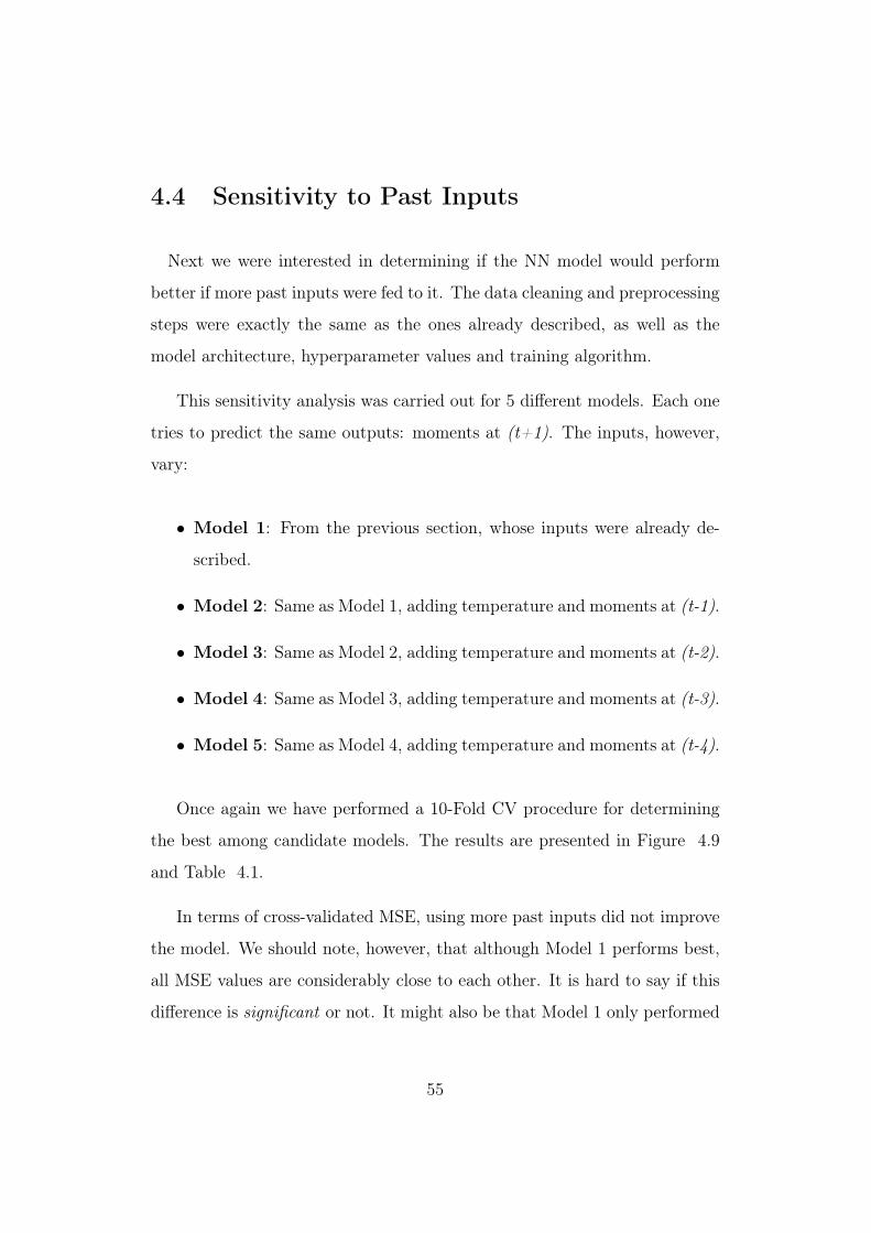
4.4 Sensitivity to Past Inputs

Next we were interested in determining if the NN model would perform

better if more past inputs were fed to it. The data cleaning and preprocessing

steps were exactly the same as the ones already described, as well as the

model architecture, hyperparameter values and training algorithm.

This sensitivity analysis was carried out for 5 different models. Each one

tries to predict the same outputs: moments at (t+1). The inputs, however,

vary:

• Model 1: From the previous section, whose inputs were already de-

scribed.

• Model 2: Same as Model 1, adding temperature and moments at (t-1).




Once again we have performed a 10-Fold CV procedure for determining

the best among candidate models. The results are presented in Figure 4.9

and Table 4.1.

In terms of cross-validated MSE, using more past inputs did not improve

the model. We should note, however, that although Model 1 performs best,

all MSE values are considerably close to each other. It is hard to say if this

difference is significant or not. It might also be that Model 1 only performed

55

best for this particular choice of hyperparameters. We will try to tackle this

sensitivity problem in a different manner in the next section.

Figure 4.9: Model sensitivity to past inputs.

Model 1 Model 2 Model 3 Model 4 Model 5

0.03326 0.03508 0.03417 0.03452 0.03499

Table 4.1: CV MSE for the 5 models considered.

4.5 Improving the Direct MLP Model: Hyper-

parameter Tuning

As we have mentioned before, the Baseline Model was used mainly as a

starting point - there was no precise reasoning behind our choices of hyper-

parameters. In this section, we will try to tune a few hyperparameters to see

56

if we can improve model performance. These parameters were described in

section 2.2.2, where we introduced ways of reducing overfitting in NN’s.

Hyperparameter tuning can be very demanding in terms of computing

power. In order to limit script running time, we have chosen 3 hyperparam-

eters to optimize:

• Number of neurons in the hidden layer: varying from 4 to 100.

• Activation function in the hidden layer: sigmoid or tanh.

• L2 Regularization parameter (α): varying from 10−8 to 10−2.

The optimization was carried out using the Optuna [62] library for Python.

Optuna lets us define an objective function, a list of optimizable parame-

ters and a range of values for these parameters. It will then try to find the

combination of parameters that minimizes (or maximizes) the objective func-

tion. Concerning our choices of activation functions, before proceeding to the

optimization problem we have experimented with other options (Gaussian,

ReLu), but quickly disconsidered them for having MSE’s in another order of

magnitude.

As we have seen during the sensitivity analysis, comparing different mod-

els can be quite difficult when dealing with a small dataset. We have thus

adopted a similar strategy to the K-Fold Cross Validation already presented:

in our definition of the objective function for Optuna, we perform a 10-Fold

CV and return the average MSE across all folds as the objective function

value. This way, Optuna will try to minimize the cross validated MSE, giv-

ing us a final model which is less dependent on train, validation and test

splits.

57

To take into account our discussion about the number of past inputs to

be used, we have performed the above optimization study for all 5 models

described in section 4.4. We have arrived at 5 optimized models, that we

compare based on the cross-validation procedure already described (Figure

4.10). The optimized parameters for each model, as well as their CV MSE,

are shown in Table 4.2.

Model nhidden activation αL2 CV MSE

1 42 tanh 2.3764× 10−6 0.01148

2 60 tanh 1.4921× 10−6 0.01100

3 66 tanh 1.9714× 10−6 0.01052

4 61 tanh 1.8547× 10−6 0.01129

5 82 tanh 3.8698× 10−6 0.01184

Table 4.2: CV MSE for the 5 models optimized with Optuna.

Figure 4.10: CV MSE for the 5 models optimized with Optuna.

Models with a tanh activation function outperformed those using sigmoid.

Our selected model is Model 3, which presented the lowest CV MSE. We

58

then retrain the model with this architecture using a conventional 80:20 split

for training and test sets, and we evaluate the optimized model via R2, with

the results shown in Figures 4.11 and 4.12.

Figure 4.11: Evaluation of the Optimized Model 3 - Training.

59

Figure 4.12: Evaluation of the Optimized Model 3 - Test.

As expected, the optimized model performs better than the baseline

model. We see that there is no overfitting, since the performances are rather

similar in training and test sets. A more practical way of evaluating models

is by using them to predict two complete experiments (Figures 4.13 and

4.14). Since our model requires 3 past inputs, and our data was initially

filtered using a moving average procedure with a window of 5 samples, pre-

diction only starts on the 9th sample of the experiment, around 10 minutes

after its start. Note that these predictions are one step ahead.

60

Figure 4.13: Evaluation of the Optimized Model - Complete experiment (1).

61

Figure 4.14: Evaluation of the Optimized Model - Complete experiment (2).

Predictions are sometimes noisy, which is probably a consequence of the

noisy measurements used as training data. A more sophisticated approach

to reducing noise might prove useful in this case. Still, the Optimized model

does a fairly good job of predicting the moments one time step ahead, even

for data points which were part of the test set. But can it also make

long-term predictions?

A first approach at studying this is straightforward: we can use model

outputs as inputs to the network at a later time step. In this way, we are

essentially creating a Recurrent Neural Network (RNN), which can look into

the future as many time steps ahead as the number of times we loop it. In

62

Figures 4.15 and 4.16 we choose a starting point, and try to predict the

next 25 minutes of the experiment solely by looping around the model.

We see that some of the moments can actually be predicted for a few

minutes before the model becomes unstable. It should be noted that the

choice of the starting point has an influence on the behavior of the predictions

throughout the rest of the experiment. Using this model in a MPC scheme

would require a longer prediction horizon. We can, however, use a different

approach for controlling the process, which is described in the next chapter.

Figure 4.15: Long-term predictions. Looping Optuna’s best model (1).

63

Figure 4.16: Long-term predictions. Looping Optuna’s best model (2).

64

Chapter 5

Inverse MLP Model

In section 2.4, we have mentioned two main ways of using NN’s for con-

trol purposes in chemical engineering: the direct and inverse modeling ap-

proaches. In the previous chapter, we have developed a preliminary direct

model of the crystallization process. This type of model can be used in a

Model Predictive Control (MPC) strategy: the model is used to make predic-

tions on the future behavior of the process, and the controller chooses the set

of values of the manipulated variable (in this case, the process temperature)

such that these predictions are close enough to a reference trajectory [16].

In the inverse modeling case, the network is the controller. It is

called an inverse model because it predicts not the process state variables,

but the value of the manipulated variable that allows to bring the process

state variables as close as possible to desired values [16]. Similarly to the

direct MLP model, we start with a baseline inverse model, described in the

next section, and then try to improve it by adjusting hyperparameters.

65

5.1 Baseline Inverse Model

The architecture of our baseline inverse model is presented in Figure 5.1.

The network has 9 inputs: the set points at time (t+1) in terms of the

moments, the current values of moments, and the previous value of process

temperature. All inputs are scaled using Standardization. The input layer

is densely connected to a hidden layer containing 8 neurons with hyperbolic

tangent activation functions and L2 Regularization with a regularization pa-

rameter α = 0.01. The hidden layer is densely connected to an output layer

with a single neuron using a linear activation function, which calculates the

control move to be implemented at current time (t).

Figure 5.1: Baseline inverse model architecture.

The NN was trained using the Adam optimizer on a Mean Squared Error

(MSE) loss function. Early Stopping was used to monitor the MSE in the

validation set (20% of the training set) and interrupt training when a reduc-

tion smaller than 10× 10−6 was observed (we use a patience parameter of 10

epochs because of the randomness involved in the training process). Model

66

design and training were carried out using the Keras library [60]. It should

be noted that, during training of the network, the set-points indicated by

µSPi (t+ 1) are replaced by the actual µi(t+ 1).

In this first case, no attempt was made to alter hyperparameters such

as number of hidden layers and neurons, neuron activation functions and

regularization parameters.

5.2 Model Evaluation

We have evaluated the baseline inverse model based on the coefficient of

determination between predicted and experimentally observed outputs. To

do so, we have taken our original dataset, split it into training and test sets

(80:20), trained the model on the training set and used it to make predictions

on both training and test sets(Figure 5.2). We have also exemplified the

model’s performance on two specific experiments (Figure 5.3).

The baseline inverse model showed good performance in predicting the

current process temperature. This performance is somewhat inferior for ex-

treme temperature values, probably because there were fewer training points

in these regions.

67

Figure 5.2: Evaluation of the baseline inverse model.

Figure 5.3: Evaluation of the baseline inverse model - Completeexperiments.

68

5.3 Improving the Inverse Model: Hyperpa-

rameter Tuning

Similarly to section 4.5, we try to further improve the performance of the

inverse model by optimizing its hyperparameters. First we define 4 different

models, which differ from one another on the inputs they receive. We adopt a

new nomenclature on this chapter: model 11 should be read as model 1-1, as

it takes past inputs at 1 time instant and future set-points at 1 time instant.

• Model 11: From the previous section, whose inputs were already de-

scribed.

• Model 12: Same as Model 11, adding moments set-points at (t+2).

• Model 21: Same as Model 11, adding moments at (t-1) and temper-

ature at (t-2).

• Model 22: Same as Model 21, adding moments set-points at (t+2).

Next, we choose the exact same parameters to optimize, namely the num-

ber of neurons in the hidden layer, the activation function in the hidden layer

and the L2 regularization parameter (α):

• Number of neurons in the hidden layer: varying from 4 to 40.

• Activation function in the hidden layer: sigmoid or tanh.

• L2 Regularization parameter (α): varying from 10−8 to 10−2.

69

We perform this optimization procedure for each of the 4 models using the

Optuna library [62], and select the best model based on the lowest CV-MSE.

Table 5.1 and Figure 5.4 summarize the results.

Model nhidden activation αL2 CV MSE

11 23 tanh 6.7515× 10−6 0.003608

12 25 tanh 2.6141× 10−6 0.002567

21 27 tanh 9.1776× 10−6 0.007016

22 34 tanh 2.7569× 10−6 0.004907

Table 5.1: CV MSE for the 4 inverse models optimized with Optuna.

Figure 5.4: CV MSE for the 4 inverse models optimized with Optuna.

Our selected model is Model 12, which presented the lowest CV MSE

and also the smallest dispersion across different folds. We have further eval-

uated this model based on the coefficient of determination between predicted

and experimentally observed outputs. To do so, we have taken our original

dataset, split it into training and test sets (80:20), trained the model on

70

the training set, and used it to make predictions on both training and test

sets(Figure 5.5). We have also exemplified the model’s performance on two

specific experiments (Figure 5.6).

Figure 5.5: Evaluation of Optuna’s best inverse mode.

Figure 5.6: Evaluation of Optuna’s best inverse model - Completeexperiments.

71

Chapter 6

Closed Loop Control

In the previous sections we have developed two distinct models based on

the crystallization data: a direct NN model of the process which predicts the

system state at (t+1) given its state at (t) and some lagged observations; and

an inverse NN model which acts as a controller of the actual process, predict-

ing the next control move to be implemented. In this section, we evaluate

this controller’s ability to make the system follow a reference trajectory. The

model we use to simulate the process is based on the solution of a Population

Balance (PB), which we describe next.

6.1 Description of the PB Model forK2SO4 Crys-

tallization

A previously developed model of the batch crystallization of K2SO4 based on

a PB [34]. The PB is a rigorous and widely adopted framework for modeling

the dynamics of dispersed system properties, such as the size distribution of

72

crystals. To track the crystal size distribution, the PB model must include

rate expressions for the crystallization mechanisms in play [44]. In the present

case, crystal nucleation and crystal growth are explicitly modeled via rate

equations. Other mechanisms, such as agglomeration and breakage, are not

modeled. In addition to the expressions for rate, energy and mass balances

are needed to express the evolution of the properties of the dispersed phase

as a function of process variables which can be manipulated. The resulting

model is composed of a system of integro partial differential equations, but

in the present case, by using the moments of the particle size distribution as

described in section 2.4, the model is transformed into a system of Ordinary

Differential Equations describing the evolution of each of the moments and

the concentration with time, µi(t) for i = 0, 1, 2, 3 and c(t), respectively.

The variation of the solvent density was neglected. The unknown parameters

of the PB model were fitted using the same dataset which was used for

the development of the NN models in the previous sections. Equation 6.1

presents the PB model which was used in our simulation.

dµ0

dt= B

dµ1

dt= GI(aµ0 + bµ1)

dµ2

dt= 2GI(aµ1 + bµ2)

dµ3

dt= 3GI(aµ2 + bµ3)

dc

dt= −3ρcαGI(aµ2 + bµ3)

(6.1)

Where,

73

B = ka exp

(kbT

)skcµkd3

GI = kg exp

(k1

T

)sk2

s = c− c∗ = c−(6.29× 10−2 + 2.46× 10−3T − 7.14× 10−6T 2

)(6.2)

And,

a = growth constant = 0.5052 [−]

b = growth constant = 7.2712 [−]

B = nucleation rate [#/cm3/min]

c = concentration of the solute [g/cm3]

ci = initial concentration of the solute [g/cm3]

c∗ = concentration of the solute in equilibrium [g/cm3]

GI = size independent growth rate [µm/min]

s = supersaturation [g/cm3]

ka = nucleation coefficient = 0.9237 [µ/min]

kb = activation energy for nucleation = -6754.8785 [K]

kc = supersaturation (s) exponent for nucleation = 0.9222 [−]

kd = µ3 exponent for nucleation = 1.3412 [−]

kg = growth coefficient = 48.0751 [µ/min]

k1 = activation energy for growth = -4921.2614 [K]

k2 = supersaturation (s) exponent for growth = 1.8712 [−]

α = volume shape factor = 1.2518 [−]

ρc = specific weight of the crystal = 2.658 [g/cm3]

74

6.1.1 Simulation of the PB Model

To show that the PB provides a good fit for the experimental data, we

show the results of simulating the model with fixed initial conditions and 2

different temperature profiles (Figures 6.1 and 6.2).

Figure 6.1: Simulation of the PB model and comparison to experimentalresults for a constant temperature profile.

75

Figure 6.2: Simulation of the PB model and comparison to experimentalresults for a varying temperature profile.

76

6.2 Control Loop

The proposed scheme for the control loop is similar to the one presented

in section 2.3 and is illustrated in Figure 6.3. The loop is initialized by

feeding the PB model with initial conditions. The PB model is then solved

for one single time-step of size 75 s, the same sampling interval used for the

experimental data acquisition. The output from the PB model is then fed to

a standard scaler along with the reference trajectory for each of the moments

µi. The scaled trajectories, current system state and previous temperature

are then fed to the NN controller, which predicts the next control move to

be implemented. The control move is inversely scaled before being fed to the

PB model for closing the loop. Note that our controller can only calculate

control moves if it receives two future reference points and one past system

state. This means our reference trajectories will be longer by two time steps

than our sequence of control moves and array of values for the moments.

Figure 6.3: Proposed scheme for the control loop.

We have already discussed the PB model and the NN controller. The

remaining piece for completing the simulation is the definition of a reference

trajectory, for which we now define a strategy.

77

6.2.1 Defining a Reference Trajectory

We have chosen to work with a few trajectories based on different types

of dynamic behaviors. We will start with a very simple trajectory, and then

work up to a few more complex ones. We will be working with the same initial

conditions as the two experiments already presented, and we will define the

desired final state of the system as being equal to the final state of the system

in one of these experiments. Equation 6.3 formalizes this.

µSPi (t∞) = µexpi (t∞) (6.3)

These trajectories will be defined for each of the moments. The initial

and final points of the different trajectories will be the same in each case,

but the evolution from the beginning to the end of each batch will be dif-

ferent. Comments about the different behaviors observed for each reference

trajectory will be made in the next section.

Constant Trajectory

Our first trajectory to be tested is a constant trajectory equal to the set

points for each of the moments (equation 6.4).

µSPi (t) = µexpi (t∞), t = 0, 1, ..., t∞ (6.4)

78

The control loop is simulated for 100 minutes (experiments duration was

approximately 60 minutes) for this trajectory. Results for the evolution of

each of the moments µi, as well as the solute concentration C and the cal-

culated temperatures (control moves) are presented in Figure 6.4. More

comments will be made later on, but we can already see that, except for µ0,

we managed to reach the desired final state.

Figure 6.4: Simulation of the control loop for a constant reference trajectory.

1st Order Trajectory

Our second choice of trajectory is a simple 1st order dynamics for each of

the moments µi, defined in a iterative way (equation 6.5). The parameter

79

γ dictates how slowly we reach the final value and can be any real number

between zero and 1. For our simulations, we used γ = 0.9. The results for

the simulation are presented in Figure 6.5. In this case, we managed to

reach the desired final state for all moments, within a small error margin.

µSPi (t0) = µi0

µSPi (t) = γµi(t− 1) + (1− γ)µSPi (t∞), t = 1, 2, ..., t∞−1

(6.5)

Figure 6.5: Simulation of the control loop for a reference trajectory definedby 1st order dynamics.

80

2nd Order Trajectory

Consider the behavior of moment µ0 in Figures 6.1 and 6.2. The simplest

dynamic model which can capture the inflection of this particular curve is a

2nd order dynamic model. The other moments don’t seem to follow a similar

behavior, but if we plot the experimental points without division by µ0 this

pattern becomes evident.

We choose a critically damped 2nd order system to model this behavior,

as the resulting equations have a single parameter τi, the time constant of

the system for µi. This approach was previously adopted in [66].

µi(t) = µi0 + (µSPi − µi0)[1−

(1 +

(t− t0τi

))]exp

(−(t− t0)

τi

)(6.6)

For defining this trajectory based on the same initial and final conditions

as for the other cases, we fit an equation described by 6.6 via least squares

to each of the moments µi using the curve_fit function from Scipy [56]. The

results are shown in figure 6.6.

We then simulate the control loop using the fitted functions as reference

trajectories (Figure 6.7). We go back to our notation of µi/µ0 for a more

straightforward comparison with previous results. Again, we are able to

arrive at approximately the desired values for every moment.

81

Figure 6.6: Defining a 2nd order reference trajectory for each of the moments.

82

Figure 6.7: Simulation of the control loop for a reference trajectory definedby 2nd order dynamics.

83

Adaptive 1st Order Trajectory

All trajectories considered up until this point were fixed a priori. We now

define an adaptive trajectory which is recalculated at each time step. The

formulation is similar to the 1st order trajectory in equation 6.5, but departs

from the actual system state at each time step. The superscript m denotes

the measured value of the variable.

µSPi (t) = µmi (t)

µSPi (t+ j) = γµmi (t+ j − 1) + (1− γ)µSPi (t∞), t = 1, 2, ..., t∞−1

(6.7)

We experimented with different values for the γ parameter, and the one

which visually presented the best results was γ = 0.6. Note that during the

simulation of the control loop, the trajectory is recalculated at each time

step. This prevents us from plotting it in the same way as in the previous

cases, as there isn’t one single trajectory for the complete experiment. For

comparison purposes, we plotted the simulation results along with a horizon-

tal line indicating the final set point for each moment (Figure 6.8). Again,

we arrive at approximately the desired values for every moment.

84

Figure 6.8: Simulation of the control loop for an adaptive 1st order referencetrajectory.

85

6.2.2 Comparison of Different Reference Trajectories

As a final topic in our analysis of this control loop, we wish to quantita-

tively compare the behavior of the controlled system under different reference

trajectories. We will base our comparison on the following criteria: the time

to reach the desired value, the error between the final system state and set

point values, and the effort in terms of the controller action.

For each reference trajectory, we can define an error between the actual

system state and the desired final state at each time instant. Let us define

the error for reference trajectory j at time t as:

εj(t) =3∑i=0

(µmi (t)− µSPi

)2 (6.8)

To account for the different scales of each variable, we will scale them

using MinMax Scaling (equation 2.5) before computing the above error. We

will define our time for each trajectory j as the time tj it takes for the system

to reach the minimum of this error, εminj .

Last, we will define our controller effort cej for reference j as a sum of

squares of control increments along each batch, up until time tj.

cej =

tj∑t=t1

(T (t)− T (t− 1))2 (6.9)

Based on these criteria, we will define a cost as the weigthed average of

the non dimensionalized forms of these 3 contributions.

86

Costj =a0tj + a1εminj + a2cej

a0 + a1 + a2

(6.10)

Where each xj is obtained by dividing the original xj by the maximum

value of xj across all different trajectories. In a practical scenario, we could

use different values for the weighting factors ai depending on what is the

main goal of the operation: time efficiency, energy efficiency or maximum

conversion. In our case, we take all a′is to be equal. The results are sum-

marized in Figure 6.9 and Table 6.1. Please note that the maximum times

do not correspond to 100 min exactly. This is due to the fact that the NN

controller needs 2 future set points as inputs, so the controller can only work

until 2 time steps before our predefined batch time.

Figure 6.9: Evolution of the error ε and the control effort ce for each referencetrajectory.

Reference Trajectory εminj εminj tj[min] tj cej[C2] cej Cost

Constant 0.0071 0.86 90 0.92 17.1 1 0.93

1st Order 0.0083 1 97.5 1 10.68 0.62 0.87

2nd Order 0.0012 0.14 80 0.82 3.53 0.21 0.39

Adaptive 0.0029 0.35 97.5 1 10.12 0.59 0.65

Table 6.1: Values for each of the criteria and cost for each reference trajectory.

87

What we are able to see is that the 2nd Order trajectory performed best

in all 3 criteria. In second place came the Adaptive Trajectory, followed by

Constant and 1st Order. The 2nd Order Trajectory resembles the trajec-

tories contained in the training set used for the development of the inverse

NN model, meaning we avoid extrapolation by feeding it to the controller.

These results might suggest that in order to achieve a desired set point with

minimum cost we should use as reference a trajectory that approximately

mimics the dynamics of the system we wish to control. More work would

have to be done in order to confirm or deny this hypothesis, but we could

further investigate this by using as a reference trajectory a possible solution

of the PB model.

88

Chapter 7

Conclusions

This project focused on the application of NN models to the identification

and control of a crystallization process. We have developed these models

using experimental data from the crystallization of K2SO4, but the method-

ology should be general enough to be applied to other batch crystallization

processes where the crystal particles are assumed to possess only one in-

ternal variable (their length). We dealt with a rather small dataset in NN

standards, which prevented us from developing more complex models such

as deep neural NN’s. Throughout model development, we have paid extra

attention to overfitting and model evaluation in order to mitigate the down-

sides of dealing with small datasets. Still, multiple improvements on the

adopted strategy would be possible.

The Direct MLP Model developed in chapter 4 performed well for the

task it was originally designed to do: predict the state of the crystallization

system in the near future given its present conditions. These predictions were

sometimes noisy, possibly due to the noisy experimental data that was used

89

for training. A more careful and sophisticated preprocessing strategy could

yield better results. We have also seen that this model becomes unstable

when we use its outputs as inputs at a later time step, which prevented us

from making accurate long-term predictions. A model which is capable of

capturing the long-term dependencies among different variables would have

to be more complex, and would require more training data as a consequence.

The limitations of this direct model prevented us from using an MPC

or Optimal Control strategy for controlling the crystallization process. We

have, thus, developed a simple strategy for control based on an inverse NN

model of the process. This controller was capable of calculating the next

control move to be implemented (i.e., the next temperature) in the scenario

where a reference trajectory for each of the moments is available.

Finally, we have investigated this controller’s performance by using a PB

as the model of our process plant. This PB model provided a good fit for

the same experimental data used in the development of the NN’s. Based on

some criteria, we have evaluated the impact of providing different reference

trajectories for the system, and noted that trajectories that approximately

resemble the dynamics of the PB model resulted in smaller errors (relative to

a final set point), batch durations and control effort. Our simulations were,

however, of limited range, considering only one initial condition. To confirm

the generality of this statement, additional trials would have to be performed

under different operating conditions.

This work is yet another example of the broad applicability of ML algo-

rithms. If enough data of good quality is available, representative models

of the underlying processes can be developed even when these are poorly

understood. This black-box approach is certainly useful in some cases, but

90

it also has downsides - specially on explainability. We have provided a few

hypotheses as to why our direct model becomes unstable, but actually con-

firming or denying these hypotheses is much harder than for the case of a

phenomenological model such as the PB. This raises the question of choos-

ing between predictive power and explainability, a common dilemma in ML

problems.

7.1 Future Work

Given the limitations mentioned above, there are quite a few possibilities

for new developments. In order to be able to train more complex models

of the dynamic behavior of the crystallization process, more data would be

needed. This data could be gathered from new experiments carried out

with different operating conditions. Alternatively, the PB model presented

in chapter 6 could be used to generate synthetic data. This approach of

generating synthetic data to train a non-parametric regression model has

found wide application, including the control of colloidal systems [67].

Regarding the extension of the model’s prediction horizon, recurrent neu-

ral networks would be a logical next step. Multiple possible architectures

exist for such NN’s. Nonlinear Autoregressive NN’s with Exogenous inputs

(NARX), for example, could help extend our prediction horizon by consid-

ering the recurrent connections during the training procedure [68], as op-

posed to after training as we have done. State-of-the-art architectures such

as LSTM and GRU networks could also yield improvements in the prediction

horizon due to their innate ability to deal with sequence data.

In possession of a better model for long-term dependencies, it would also

91

be possible to investigate different control paradigms such as the MPC ap-

proach described in section 2.3. This could provide a more robust framework

for controlling crystallization processes as opposed to the relatively simplistic

approach taken in the present work.

Finally, our conclusions regarding the choice of reference trajectory for

control purposes would require more investigation under different operating

conditions. Given the interesting results obtained for the 2nd Order Trajec-

tory, it might also be interesting to study reference trajectories that are even

more similar to possible solutions of the PB model.

92

Bibliography

[1] J. D. Seader and Ernest J. Henley. Separation Process Principles. John

Wiley & Sons, 2006.

[2] Doraiswami Ramkrishna. Population Balances: Theory and Applica-

tions to Particulate Systems in Engineering. Academic Press, 200.

[3] Trevor Hastie, Robert Tibshirani, and Jerome Friedman. The Eele-

ments of Statistical Learning. Springer, 2008.

[4] Leslie Pack Kaelbling, Michael L. Littman, and Andrew W. Moore.

“Reinforcement Learning: A Survey”. In: Journal of Artificial Intelli-

gence Research 4 (1996), pp. 237–285.

[5] Sepp Hochreiter and Jurgen Schmidhuber. “Long Short-TermMemory”.

In: Neural Computation 8.8 (1997), pp. 1735–1780.

[6] Kyunghyun Cho et al. “Learning Phrase Representations using RNN

Encoder-Decoder for Statistical Machine Translation”. In: CoRR abs/1406.1078

(2014).

[7] Ian Goodfellow, Yoshua Bengio, and Aaron Courville. Deep Learning.

MIT Press, 2016.

93

[8] Data Science Academy. Deep Learning Book. Available at http://

deeplearningbook . com . br / aprendizado - com - a - descida - do -

gradiente (03/13/2021).

[9] Andriy Burkov. The Hundred-Page Machine Learning Book. Andriy

Burkov, 2019.

[10] David Rumelhart, Geoffrey Hinton, and Ronald Williams. “Learning

representations by back-propagating errors”. In: Nature 323 (1986),

pp. 533–536.

[11] Sutton Monro Herbert Robbins. “A Stochastic Approximation Method”.

In: Annals of Mathematical Statistics 22.3 (1951), pp. 400–407.

[12] J. Kiefer and J. Wolfowitz. “Stochastic Estimation of the Maximum

of a Regression Function”. In: Annals of Mathematical Statistics 23.3

(1952), pp. 462–466.

[13] Diederik P. Kingma and Jimmy Ba. Adam: A Method for Stochastic

Optimization. 2017. arXiv: 1412.6980 [cs.LG].

[14] John McGonagle, George Shaikouski, and Cristopher Williams. Back-

propagation. Available at https://brilliant.org/wiki/backpropagation

(03/13/2021).

[15] Christopher M. Bishop. Pattern Recognition and Machine Learning.

Springer, 2006.

[16] Maurício Bezerra de Souza Jr. “Redes Neuronais Multicamadas Apli-

cadas A Modelagem e Controle de Processos Químicos”. PhD thesis.

COPPE/UFRJ, 1993.

[17] D. R. Bauhman and Y. A. Liu. Neural Networks in Bioprocessing and

Chemical Engineering. Academic Press, 1995.

94

[18] Michael A. Hanson and Dale E. Seborg. Nonlinear Process Control.

Prentice Hall PTR, 1997.

[19] N. V. Bhat and T. J. McAvoy. “Use of neural nets for dynamic modeling

and control of chemical process systems”. In: Proceedings of American

Control Conference (1989), pp. 1336–1341.

[20] E. Hernandez and Y. Arkun. “A study of the control relevant properties

of backpropagation neural net models of nonlinear dynamic systems.”

In: Computers & Chemical Engineering 4 (1992), pp. 227–240.

[21] J. Saint-Donat, N. Bhat, and T. J. McAvoy. “Neural net based model

predictive control.” In: International Journal of Control 6 (1991), pp. 1453–

1468.

[22] J. Leonard and M. Kramer. “Radial basis functions networks for clas-

sifying process faults”. In: IEEE Control Systems Magazine (1991),

pp. 31–38.

[23] L. H. Ungar, B. A. Powell, and S. N. Kamens. “Adaptive networks

for fault diagnosis and process control”. In: Computers & Chemical

Engineering 4/5 (1990), pp. 561–572.

[24] M. A. Kramer. “Autoassociative neural networks”. In: Computers &

Chemical Engineering 4 (1992), pp. 313–328.

[25] D. Dong and T. J. McAvoy. “Nonlinear principal component analysis

- based on principal curves and neural networks”. In: Computers &

Chemical Engineering 1 (1996), pp. 65–78.

[26] Yoh-Han Pao, Stephen M. Phillips, and Dejan J. Sobajic. “Neural-net

computing and the intelligent control of systems”. In: International

Journal of Control 56.2 (1992), pp. 263–289.

95

[27] A. G. Jones. Crystallization Process Systems. Butterworth-Heinemann,

2002.

[28] R. J. Davey and J. Garside. From Molecules to Crystallizers - An In-

troduction to Crystallization. Oxford University Press, 2006.

[29] J. M. Schall and A. S. Myerson. “Solutions and solution properties”. In:

Handbook of Industrial Crystallization (3rd Edition). Ed. by A. Myer-

son, D. Erdemir, and S. Lee. Cambridge University Press, 2019, pp. 1–

31.

[30] J. W. Mullin. Crystallization. Butterworth-Heinemann, 2001.

[31] D. Erdemir, A. Y. Lee, and A. S. Myerson. “Crystal Nucleation”. In:


son, D. Erdemir, and S. Lee. Cambridge University Press, 2019, pp. 1–

31.

[32] S. Karthika, T. K. Radhakrishnan, and P. A. Kalaichelvi. “A review of

classical and nonclassical nucleation theories”. In: Crystal Growth and

Design 11 (2016), pp. 6663–6681.

[33] M. Giulietti et al. “Industrial Crystallization and Precipitation from

Solutions: State of the Technique”. In: Brazilian Journal of Chemical

Engineering 4 (2001), pp. 423–440.

[34] Marcellus G. F. de Moraes. Modelagem, monitoramento e controle do

tamanho e forma de cristais em processos de cristalização. Exame de

Qualificação de Doutorado. 2019.

[35] A. S. Myerson and R. Ginde. “Crystal growth and nucleation”. In:


son and S. Lee D. Erdemir. Cambridge University Press, 2019, pp. 1–

31.

96

[36] A. Lewis et al. Industrial Crystallization: Fundamentals and Applica-

tion. Cambridge Univeristy Press, 2015.

[37] A. A. Noyes and W. R. Whitney. “The Rate of Solution of Solid Sub-

stances in their Own Solutions”. In: Journal of the American Chemical

Society 12 (1987), pp. 930–934.

[38] A. Y. Lee, D. Erdemir, and A. S. Myerson. “Crystal growth and nu-

cleation”. In: Handbook of Industrial Crystallization (3rd Edition). Ed.

by A. Myerson, D. Erdemir, and S. Lee. Cambridge University Press,

2019, pp. 1–31.

[39] U. Fasoli and R. Conti. “Crystal breakage in a mixed suspesion crys-

tallizer”. In: Crystal Research and Technology 8 (1973), pp. 931–946.

[40] K. A. Berglund. “Analysis and Measurement of Crystallization Utiliz-

ing the Population Balance”. In: Handbook of Industrial Crystallization

(3rd Edition). Ed. by A. Myerson, D. Erdemir, and S. Lee. Cambridge

University Press, 2019, pp. 1–31.

[41] M. Brunsteiner et al. “Towards a Molecular Understanding of Crystall

Agglomeration”. In: Crystal Growth & Design 1 (2006), pp. 3–16.

[42] P. Barrett et al. “A review of the use of process analytical technology

for the understanding and optimization of production in batch crys-

tallization processes”. In: Organic Process Research & Development 3

(2005), pp. 348–355.

[43] Alan Randolph. Theory of Particulate Processes: Analysis and Tech-

niques of Continuous Crystallization. Academic Press, 1971.

[44] Daniel J. Griffin et al. “Data-Driven Modeling and Dynamic Program-

ming Applied to Batch Cooling Crystallization”. In: Industrial & En-

gineering Chemistry Research 55 (2016), pp. 1362–1372.

97

[45] Daniel J. Griffin et al. “Mass-Count Plots for Crystal Size Control”. In:

Chemical Engineering Science 137 (2015), pp. 338–351.

[46] Martha A. Grover et al. “Optimal feedback control of batch self-assembly

processes using dynamic programming”. In: Journal of Process Control

88 (2020), pp. 32–42.

[47] Rasmus Fjordbak Nielsen et al. “Hybrid machine learning assisted mod-

elling framework for particle processes”. In: Computers & Chemical En-

gineering 140 (2020), p. 106916.

[48] P. Lauret, H. Boyer, and J. Gatina. “Hybrid Modelling of the Sucrose

Crystal Growth Rate”. In: International Journal of Simulation Model-

ing 21.1 (2001), pp. 23–29.

[49] V. Galvanauskas, P. Georgieva, and S. F. D. Azevedo. “Dynamic Op-

timisation of Industrial Sugar Crystallization Process based on Hy-

brid (mechanistic+ANN) Model”. In: International Joint Conference

on Neural Networks (2006).

[50] Yanmei Meng et al. “Hybrid modeling based on mechanistic and data-

driven approaches for cane sugar crystallization”. In: Journal of Food

Engineering 257 (2019), pp. 44–55.

[51] Youngjo Kim et al. “Unification of an empirical and a physically-based

approach to crystallization monitoring”. In: 2018 Annual American

Control Conference (ACC). 2018, pp. 5106–5112. doi: 10.23919/ACC.

2018.8430977.

[52] Pedro Abreu et al. “Investigação da Análise de Imagens como Ferra-

menta para a Cristalização de K2SO4 em Batelada com Semeadura”.

In: Aug. 2019, pp. 2352–2358.

98

[53] Marcellus Moraes, Maurício de Souza Jr, and Argimiro Secchi. “Dy-

namics and MPC of an Evaporative Continuous Crystallization Pro-

cess”. In: Jan. 2018, pp. 997–1002. isbn: 9780444642356.

[54] Caio Marcellos et al. “Optimal Operation of Batch Enantiomer Crys-

tallization: From Ternary Diagrams to Predictive Control”. In: AIChE

Journal 64 (Nov. 2017).

[55] S. van der Walt, S. C. Colbert, and G. Varoquaux. “The NumPy Array:

A Structure for Efficient Numerical Computation”. In: Computing in

Science Engineering 13.2 (2011), pp. 22–30.

[56] Pauli Virtanen et al. “SciPy 1.0: Fundamental Algorithms for Scientific

Computing in Python”. In: Nature Methods 17 (2020), pp. 261–272.

[57] Wes McKinney. “Data structures for statistical computing in Python”.

In: Proceedings of the 9th Python in Science Conference (2020), pp. 56–

61.

[58] J. D. Hunter. “Matplotlib: A 2D graphics environment”. In: Computing

in Science and Engineering 9.3 (2007), pp. 90–95.

[59] Michael Waskom. “Seaborn”. In: Zenodo (2020).

[60] François Chollet. Keras. Available at https://github.com/fchollet/

keras\%7D\%7D(03/20/2021).

[61] F. Pedregosa et al. “Scikit-learn: Machine Learning in Python”. In:

Journal of Machine Learning Research 12 (2011), pp. 2825–2830.

[62] T. Akiba et al. “Optuna: A Next-generation Hyperparameter Optimiza-

tion Framework”. In: Proceedings of the 25th International Conference

on Knowledge Discovery and Data Mining (2019).

99

[63] J. Brownlee. How to transform data to better fit the normal distribu-

tion. Available at https://machinelearningmastery.com/how-to-

transform-data-to-fit-the-normal-distribution/ (04/10/2021).

[64] Power Transform. In: Wkipedia, the free encyclopedia. Available at

https://en.wikipedia.org/wiki/Power\_transform (04/10/2021).

[65] Lawrence R. Rabiner and Bernard Gold. Theory and Application of

Digital Signal Processing. Prentice-Hall, 1975.

[66] E. F. Fonseca et al. “A Hybrid Neural Model for the Production of Sor-

bitol and Gluconic Acid Using Immobilized Zymomonas mobilis Cells”.

In: Latin America Applied Research 34 (2004), pp. 187–193.

[67] Xun Tang, Michael A. Bevan, and Martha A. Grover. “The construction

and application of Markov state models for colloidal self-assembly pro-

cess control”. In: Molecular Systems Design and Engineering 2 (2017),

pp. 78–88.

[68] Dale E. Seborg, Thomas F. Edgar, and Duncan A. Mellichamp. Process

Dynamics and Control. John Wiley & Sons Inc., 2004.

100

Date post:	09-Dec-2021
Category:	Documents
Upload:	others
View:	3 times
Download:	0 times

Dynamic Modeling and Control of a Crystallization Process ...

Documents