Dynamic modelling of flexibly supported gears using iterative convergence of tooth mesh stiffness Song Xue, Ian Howard* Department of Mechanical Engineering, Curtin University, Bentley, Western Australia, Australia Department of Mechanical Engineering, Curtin University of Technology, GPO Box U1987, Perth, WA 6845, Australia * Corresponding author. Phone: (+61) 89266 7047. E-mail: [email protected]Abstract: This paper presents a new gear dynamic model for flexibly supported gear sets aiming to improve the accuracy of gear fault diagnostic methods. In the model, the operating gear centre distance, which can affect the gear design parameters, like the gear mesh stiffness, has been selected as the iteration criteria because it will significantly deviate from its nominal value for a flexible supported gearset when it is operating. The FEA method was developed for calculation of the gear mesh stiffnesses with varying gear centre distance, which can then be incorporated by iteration into the gear dynamic model. The dynamic simulation results from previous models that neglect the operating gear centre distance change and those from the new model that incorporate the operating gear centre distance change were obtained by numerical integration of the differential equations of motion using the Newmark method. Some common diagnostic tools were utilized to investigate the difference and comparison of the fault diagnostic results between the two models. The results of this paper indicate that the major difference between the two diagnostic results for the cracked tooth exists in the extended duration of the crack event and in changes to the phase modulation of the coherent time synchronous averaged signal even though other notable differences from other diagnostic results can also be observed. Keyword: Gear dynamics, Mesh stiffness, Tooth fault, Gear fault diagnostics, phase modulation
Transcript
Dynamic modelling of flexibly supported gears using iterative
convergence of tooth mesh stiffness
Song Xue, Ian Howard*
Department of Mechanical Engineering, Curtin University, Bentley, Western Australia, Australia Department of Mechanical Engineering, Curtin University of Technology, GPO Box U1987, Perth,
where rap is the addendum radius of the pinion and rag is the addendum radius of the gear and m is the gear module. The operating gear contact ratio 𝑚𝑚𝑝𝑝
′ will become,
𝑚𝑚𝑝𝑝′ =
�𝑟𝑟𝑎𝑎𝑝𝑝2 − 𝑟𝑟𝑝𝑝2 + �𝑟𝑟𝑎𝑎𝑔𝑔2 − 𝑟𝑟𝑔𝑔2 − 𝑑𝑑′ sin𝛼𝛼′
𝜋𝜋 ∙ 𝑚𝑚 ∙ cos𝛼𝛼′, (8)
The gear contact ratio is closely related to the variation in gear mesh stiffness as the proportions of the single
and double contact zones are determined by the contact ratio mp, as shown in Fig. 2. Tm is the gear mesh period.
The gear mesh stiffness Kmb is said to be shaft phase variant mesh stiffness as it is a function of the shaft rolling
angle θp [4]. From equation (7) and (8), it was found that the gear centre distance variation has great impact on
gear pressure angle and gear contact ratio. As the gear mesh stiffness property was also dependent on the gear
contact ratio, it can be concluded that the gear centre distance variation would also have great impact on the gear
mesh stiffness. Because the variation of the gear mesh stiffness is the main vibration generation mechanism in
gear systems, the gear centre distance variation should also be considered when analysing the gear dynamic
responses. Section 3 presents the study of the gear mesh stiffness with different gear centre distance using the
FEA method.
Fig. 2 Gear mesh stiffness with single and double contact zones
2.2 Equation of gear motion
A simplified transverse-torsional gear dynamic model was used in this research and as the focus of this study is
to investigate the gear centre distance variation impact on gear dynamic motion instead of the whole system
effect, only a single one-stage gear system was modelled with the motor and load. The input load Tin was
provided by the motor and was assumed to be constant. The motor shaft and the shaft that the pinion mounts on
are coupled with a flexible coupling. The output load Tout was applied to the gear and it was assumed to depend
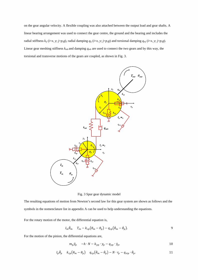
on the gear angular velocity. A flexible coupling was also attached between the output load and gear shafts. A
linear bearing arrangement was used to connect the gear centre, the ground and the bearing and includes the
The detailed method of calculating gear torsional mesh stiffness can be found in [11]. Using the strategy
mentioned in [11], one FEA spur gear model with one pinion and one gear can be obtained. The whole gear
model can then be moved intentionally in the vertical direction with a distance increment of ∆d, as shown in Fig.
4. This results in a new gear centre distance d+∆d, where distance increment ∆d will also introduce a backlash
ΔB=2·Δd·tanα between the pinion involute profile and the gear involute profile. As a result, an imposed
displacement of Δd·tanα/rpp can be introduced to the pinion gear hub to eliminate the backlash ΔB. After
rotation, the adaptive re-mesh method can be used at each contact position. The weak spring connected with the
pinion hub node method is also needed followed by the element birth & death command to disable the weak
spring after the pinion moves to be just in contact with the gear profile.
Fig. 4 FEA gear model with distance increment
The initial contact point was selected to be at the pitch mesh position and the pinion gear hub was constrained in
the radial direction while the gear hub was constrained in both tangential and radial directions at each mesh
point. An input load Tp=100Nm was applied to the pinion hub and different distance increments were then
applied to the gear. In this study, several different distance increments were considered, Δd=0mm, Δd=0.5mm
and Δd=1mm. The corresponding FEA shaft phase-variant gear mesh stiffness results are shown in Fig. 5.
Fig. 5 FEA results with different gear distance, (a) combined torsional mesh stiffness, (b) load sharing ratio.
Fig. 5(a) describes the combined shaft phase-variant gear mesh stiffness results at each meshing position. It is
apparent that the overall gear mesh stiffness amplitude decreases due to the increase of the gear centre distance
for both single contact and double contact zones. What is most interesting in this curve set is the change of the
proportions of the single and double contact zones, which will result in a phase lag when the adjacent gear tooth
comes into mesh. This mesh lag can also be seen in the load sharing ratio plot, in Fig 5(b). With the increase of
the gear centre distance, the length of the single contact zone, whose length is (2-mp)Tm, increases while the
length of the double contact zone, whose length is (mp-1)Tm, decreases accordingly. Traditionally, only the K00
curve will be interpolated into the gear dynamic equation when the gear dynamic response was studied, no
matter what the gear centre distance variation was. In other words, the gear mesh stiffness was assumed to be
only the function of the pinion rolling angle. However, if the gear centre distance increment varies from 0mm to
1mm during the operation, the mesh stiffness will have to vary between K00 and K10 accordingly, which will
result in a dramatically different dynamic response.
A 5 mm crack at the root of one tooth can also be created in the FEA model of the gear pair shown in Fig. 4.
The LEFM (linear elastic fracture mechanics) assumption was used in the tooth crack model. The resultant mesh
stiffness results with a 5 mm crack for a 1 mm gear centre distance variation can be found in Fig. 6.
Fig. 6 Combined torsional mesh stiffness comparison with different centre distance increment and a 5mm tooth root crack.
Compared to the healthy gear stiffness curve (K00), the faulted gear mesh stiffness (KC005) decreased
considerably due to the crack fault on the tooth. This stiffness reduction can be found in many available
publications [12, 13]. However, due to the increment of the gear centre distance, the length of the single contact
zone is expected to be larger than the nominal value and as a result, compared to the healthy gear stiffness curve
(K00), curve KC105 would experience a stiffness reduction as well as a change of the stiffness proportion. The
dynamic gear system response caused by curve KC105 would therefore be expected to be different from the
dynamic response caused by curve KC005.
4 Numerical simulation and result discussion
To solve the matrix dynamic equations of the gear pair, a procedure based on the direct time-integration
Newmark method was developed in this study and the flow chart of the gear dynamic simulation scheme can be
found in Fig. 7. As shown in the flow chart, the parameters for the Newmark method were initialized at the
beginning, and the gear centre distance d(t) was set to be equal to the designed gear centre distance as there is
no input load applied to the system. Based on the initial values of pinion rotation angle and gear centre distance,
the stiffness K(θ, d(t)) can be evaluated accordingly and then the stiffness matrix for the Newmark method can
be assembled. The gear system responses can be calculated for the time step t+∆t and subsequently, the new
gear centre distance d(t+∆t) can be calculated using equation (4). However, as the gear centre distance can have
great impact on the gear dynamic response, an inspection at each time step should be made to examine whether
the gear centre distance has converged or not. Initially, the iteration step m is set to be 0 and b1(m) is set to be
the gear centre distance at time step t and b2(m) is set to be the gear centre distance at time step t+∆t. The
|b1(m)-b2(m)| convergence criterion was used in this study and the value of eps was chosen to be 0.1μm. If the
convergence criterion result is smaller than eps, the procedure will then continue for the next time step. If not,
the procedure will pass the value of b2(m) to b1(m) and then re-evaluate the gear mesh stiffness based on b1(m).
As a result, the gear system responses need to be re-calculated for time step t+∆t and the gear centre distance for
time step t+∆t will be re-calculated as well. If the result satisfies the convergence condition, that is, it is less
than eps, the procedure will keep the gear responses and if not, the calculation will be forced into the iteration
again until it satisfies the convergence criteria.
Fig. 7 Flowchart of iterative numerical gear dynamic time integration
4.1 Gear design parameter analysis
From the MATLAB program, the gearbox system was simulated over several seconds, after which the initial
transient start-up phase has decayed away and the steady-state conditions were obtained. The gear mesh
stiffness curve due to a 5 mm crack was then incorporated into the differential equations of motions. The
presence of the crack can introduce some transient disturbance into the gear system affecting the gear centre
distance, even though the gear system is still in the steady-state vibration stage. Fig. 8 illustrates the variation of
gear centre distance change, gear pressure angle and gear contact ratio with the presence of the gear tooth root
crack during the steady-state stage.
Fig. 8 The effect of the gear crack on gear design parameters, (a) gear centre distance change (G.C.D.C.), (b) gear pressure angle (G.P.A.), (c) gear contact ratio (G.C.R.).
From Fig. 8, it is apparent that all the gear design parameters vary during the simulation. The gear centre
distance change was calculated as the instantaneous gear centre distance minus the designed gear centre distance
(d (t)-d). During this stage, the gear centre distance stabilized at the new value, which was around 1.07mm away
from its designed value. The gear pressure angle stabilized at around 21.18º, which was 1.18º away from its
designed value. The gear contact ratio stabilized at around 1.43, which was 0.17 away from its designed value.
The presence of the crack can be seen in all the results at approximately t=0.049s. It was noted that the gear
crack could change the gear centre distance from its newly stable value (139.07mm), but after the crack event,
the gear centre distance again went back to its stable value. The gear pressure angle and gear contact ratio were
also affected by the presence of the crack, but similarly, they both went back to their stable response values after
the crack event. The iteration process due to the crack can also be obtained and the resultant gear mesh stiffness
behaviour is shown in Fig. 9. In Fig. 9(a), the red line shows the value of |b1(m)-b2(m)| before the iteration and
the black line illustrates the value of |b1(m)-b2(m)| after the iteration.
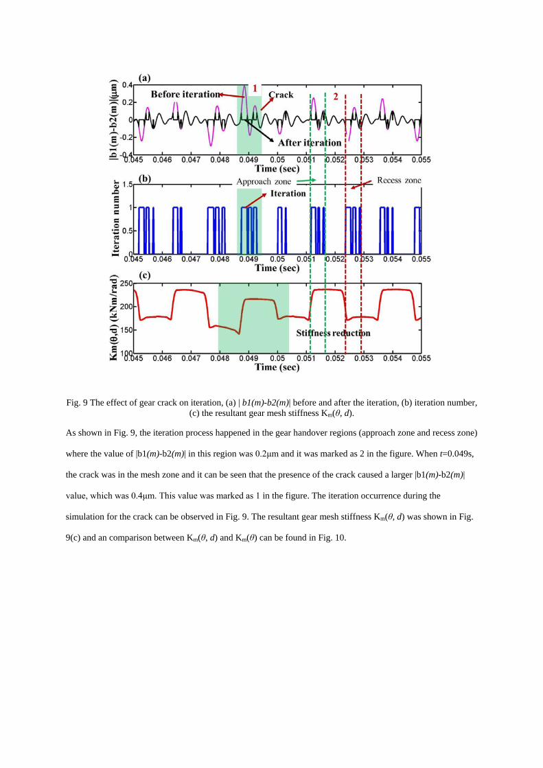
Fig. 9 The effect of gear crack on iteration, (a) | b1(m)-b2(m)| before and after the iteration, (b) iteration number, (c) the resultant gear mesh stiffness Km(θ, d).
As shown in Fig. 9, the iteration process happened in the gear handover regions (approach zone and recess zone)
where the value of |b1(m)-b2(m)| in this region was 0.2μm and it was marked as 2 in the figure. When t=0.049s,
the crack was in the mesh zone and it can be seen that the presence of the crack caused a larger |b1(m)-b2(m)|
value, which was 0.4μm. This value was marked as 1 in the figure. The iteration occurrence during the
simulation for the crack can be observed in Fig. 9. The resultant gear mesh stiffness Km(θ, d) was shown in Fig.
9(c) and an comparison between Km(θ, d) and Km(θ) can be found in Fig. 10.
Fig. 10 Comparison of faulted gear mesh stiffness variation with or without the effect of gear centre distance variation. Km(θ) is the mesh stiffness without considering centre distance variation, Km(θ, d) is the mesh
stiffness with centre distance variation.
Compared with the variation of Km(θ) obtained from neglecting centre distance changes, it was found that the
reduction of the gear mesh stiffness caused by the crack, Km(θ, d), was larger when the centre distance changes
were used. This different decrease of the mesh stiffness would result in a different gear dynamic response due to
the presence of the gear tooth crack.
4.2 Gear fault diagnostic result analysis
Two models have been used in this study. Model I is the gear system incorporating the stiffness curve Km(θ) and
Model II is the gear system incorporating the stiffness curve Km(θ, d). After the initial transient start-up was
observed to have decayed away, the input pinion angular velocity �̇�𝜃𝑝𝑝, gear vertical velocity �̇�𝑦𝑔𝑔 as well as the
transmission error θp-θg have been obtained to compare the difference of the diagnostic results. The diagnostic
algorithms which are commonly used for gearbox vibration analysis were used on the simulation results from
the two models. These diagnostic techniques include coherent time synchronous averaging, RMS spectrum,
residual signal, narrow band envelope, amplitude modulation, phase modulation and analytic signal plots.
Fig. 11 shows the results of the coherent time synchronous averaged signal, where the gear vertical velocity,
pinion angular velocity and transmission error are resampled into equispaced phase data and then averaged over
several rotations of the shaft. The dynamic motions from model I (without considering the effect of gear centre
distance) are shown in the left column and those from model II (including the effect of gear centre distance) are
shown in the right column.
Fig. 11 Dynamic motion over one complete revolution from model I (left column) and from model II (right column). (a) Output gear vertical velocity �̇�𝑦𝑔𝑔; (b) Input pinion angular velocity �̇�𝜃𝑝𝑝; (c) Transmission error θp-θg.
As shown in Fig. 11, the presence of the crack can be seen in all the results at approximately 170° rotation of the
shaft and the inclusion of the gear centre distance effect can be seen to slightly change the simulation results as
the crack goes through the mesh. It can be oberved that the inclusion of the centre distance iteration effect
increases the magnitude of the dynamic motions, especially in the gear vertical velocity and in the pinion
torsional velocity. A closer look at the simulation results can be found in table 2, which provides the mean,
standard deviation (STD), skewness, kurtosis and crest factor of the signals.
Table 2 Comparison of diagnostic results for models I and II
Fig. 12 shows the results of the RMS spectra, which are based on the time averaged signals obtained in Fig. 11.
As the time signal covers exactly one shaft revolution, the RMS spectral results are presented in terms of shaft
orders. The dynamic motions from model I (without considering the effect of gear centre distance) are shown in
the left column and those from model II (including the effect of gear centre distance) are shown in the right
column.
Fig. 12 RMS spectrum amplitude results from model I (left column) and from model II (right column). (a) Output gear vertical velocity �̇�𝑦𝑔𝑔; (b) Input pinion angular velocity �̇�𝜃𝑝𝑝; (c) transmission error θp-θg.
As shown in Fig. 12, both RMS spectrum plots are dominated by strong gear mesh sidebands and the inclusion
of the gear distance effect started to change the frequency content from the second gear mesh frequency, which
is 46 shaft orders. It can be oberved that inclusion of this effect reduces the amplitude of the second and fourth
mesh harmonic in all three spectrum plots, while increasing the third. For example, in the RMS spectrum of the
output gear vertical velocity, the amplitude at the second harmonic from model I was around -25.28 dB and the
result from model II was around -31.36 dB. A close look at the gear mesh sideband can be achieved by
examining the residual signal, which removes all the gear mesh harmonics and only includes the sideband in the
RMS spectra and then uses the inverse Fourier transform to obtain the signal in the time domain, as shown in
Fig. 13.
Fig. 13 shows the results of the residual signal and it can be noted that the presence of the crack can be observed
in all three results and the inclusion of the gear centre effect changes the residual signal waveform shape
significantly. However, it should be noted that the inclusion of this gear centre effect gives a smaller kurtosis
value in the output gear residual signal (62.29 vs 52.47) and the input pinion residual signal (47.60 vs 41.43).
Moreover, the overall magnitude of the transmission error increases slightly and the inclusion of this gear centre
effect gives a higher kurtosis value here (5.71 vs 6.04).
Fig. 13 Residual signal for model I (left column) and from model II (right column). (a) Output gear vertical velocity �̇�𝑦𝑔𝑔; (b) Input pinion angular velocity �̇�𝜃𝑝𝑝; (c) transmission error θp-θg.
The simultaneous representation in both time and frequency domains offers important advantages for the
analysis of non-stationary signals [14]. The Wigner-Ville distribution (WVD) is one of the well known time-
frequency methods and its application to the detection of the gear damage has been widely described in
publications [15]. By applying a suitable window function in the time domain, the cross-terms in the WVD can
be attenuated and the windowed version of the WVD is often called the pseudo Wigner-Ville distribution
(PWVD) [15]. In this research, the PWVD technique was employed to further compare the signals from model I
and model II. Note that the ‘shaft domain’ synchronous signal averages with the rotation ‘angle’ being
analogous to ‘time’ and the frequency was therefore in terms of shaft order [15].
Fig. 14 shows the PWVD of the output gear velocity signal. The synchronous signal averages generated in Fig.
11(a) were used as input for the PWVD and Fig. 14 (a) shows the PWVD for the gear signal in model I and Fig.
14 (b) shows the PWVD for the gear signal in model II. The pinion has 23 teeth, and as expected, the PWVD
gave a vibration signal with major components at the tooth mesh frequency (23 orders) and its harmonics (n×23)
as shown in the figure. If no fault existed in the gear system, a uniform distribution would be expected in the
PWVD whilst once a fault happens, the energy distribution would be expected to change correspondingly and
these energy redistributions are largely because of the amplitude modulation and phase modulation induced by
the gear fault [15]. Even though the cross-terms can still be observed in both figures, compared with the result in
Fig. 14(a), Fig. 14 (b) was observed to have wider energy distribtuted through the shaft rotation angle when the
crack occured between 150° and 200°.
Fig. 14 The Pseudo Wigner-Ville distribution (PWVD) of the output gear vertical velocity �̇�𝑦𝑔𝑔, (a) PWVD of the signal from model I; (b) PWVD of the signal from model II.
The limitation of using the synchronous averaged signal for PWVD analysis was that the gear mesh harmonics
were found to dominate the distribution and removing the components at the meshing harmonics can increase
the sensitivity to energy changes related to the damage [16]. Further analysis can be found in Fig. 15, which
presents the PWVD analysis of the residual signal of the output gear vertical velocity �̇�𝑦𝑔𝑔. A much clearer
difference in the energy distribution pattern can be observed and these results further indicated that the highest
energy occurred around the fifth mesh harmonic.
Fig. 15 The Pseudo Wigner-Ville distribution (PWVD) of the residual output gear vertical velocity �̇�𝑦𝑔𝑔, (a) PWVD of the signal from model I; (b) PWVD of the signal from model II.
The non-uniformly distributed energy is closely related to the amplitude modulation and phase modulation, so
the narrowband envelope, amplitude modulation and phase modulation techniques were further used for
subsequent analysis. As the highest energy in Fig. 15 occurred around the fifth mesh harmonic, it was chosen for
the demodulation process and a bandwidth of 22 shaft orders (±11) was used for the analysis.
Fig. 16 shows the results of the narrow band envelope, amplitude modulation and phase modulation from the
output gear vertical velocity �̇�𝑦𝑔𝑔, including the crack. The left column shows the results from model I and the
right column shows the results from model II. The presence of the crack can be clearly observed in both models
at around 170° rotation of the shaft whilst the diagnostic results from model II are found to be different with
those from model I in several ways even though the kurtosis value in the narrow band envelope is almost
identical (14.65 vs 14.28). First, the overall value in the amplitude modulation of model I is less than half of the
value of model II. Second, although the presence of the crack can be observed in both phase modulation results,
a striking observation can be found in the overall value of the phase modulation. The phase modulation result
from model I stays around 40° whilst the phase modulation result from model II stays around -130°.
Fig. 16 Narrowband envelope, amplitude modulation and phase modulation of the output gear vertical velocity �̇�𝑦𝑔𝑔 from model I (left column) and from model II (right column).
The amplitude and phase modulation can be further observed in the analytical signal obtained from the fifth
mesh harmonic, as shown in Fig. 17. It can be found in the figure that the inclusion of the gear centre distance
effect provides a significant influence on the amplitude and phase modulation, especially the phase. The kurtosis
values for the amplitude modulation of model I and model II were 14.25 and 12.79 respectively. The kurtosis
values for the phase modulation of the model I and model II were 7.98 and 6.3 respectively.
Fig. 17 The analytic signal from the fifth mesh harmonic of the output gear vertical velocity �̇�𝑦𝑔𝑔.
Fig. 18 shows the PWVD of the input pinion angular velocity residual signal. Fig. 18 (a) shows the PWVD for
the pinion residual signal in model I and Fig. 18 (b) shows the PWVD for the pinion residual signal in model II.
Similar with the pattern in Fig. 15, the highest energy can be observed at the fifth mesh harmonic between 150°
and 200°. A wider energy distribution due to the localised tooth root crack on the pinion can be found in the
PWVD of model II, which indicated that the results from model II has different amplitude and phase modulation.
Fig. 18 The Pseudo Wigner-Ville distribution (PWVD) of the input pinion angular velocity θ̇p residual signal (a) PWVD of the residual signal from model I; (b) PWVD of the residual signal from model II.
Fig. 19 shows the results of the narrow band envelope, amplitude modulation and phase modulation obtained
from the demodulation of the input pinion torsional velocity �̇�𝜃𝑝𝑝, about the fifth mesh harmonic. The left column
shows the results from model I and the right column shows the results from model II. Similar trends as observed
in Fig. 16 can be found in these results. The overall magnitude of the amplitude modulation of model II is
slightly higher than that from model I. The most striking results can still be found in the phase modulation as the
phase modulation result from model I stays around -110° while the result from model II stays around 80°.
Fig. 19 Narrowband envelope, amplitude modulation and phase modulation of the input pinion torsional velocity �̇�𝜃𝑝𝑝 from model I (left column) and from model II (right column).
The amplitude and phase modulation can be further observed in the analytical signal obtained from the fifth
mesh harmonic, as shown in Fig. 20. It can be seen in the figure that the inclusion of the gear centre distance
effect provides a significant influence on the amplitude and phase modulation. The kurtosis values for the
amplitude modulation from model I and model II are 14.25 and 12.71 respectively. The kurtosis values for the
phase modulation from model I and model II are 7.74 and 6.27 respectively.
Fig. 20 The analytic signal from the fifth mesh harmonic of the input pinion torsional velocity �̇�𝜃𝑝𝑝.
Fig. 21 shows the PWVD of the transmission error residual signal. Fig. 21 (a) shows the PWVD for the
transmission error residual signal in model I and Fig. 21 (b) shows the PWVD for the transmission error residual
signal in model II. A strong DC component can be found when initially ploting the spectrum and as a result, this
DC component needs to be eliminated. Unlike the energy distribution pattern shown in Fig. 15 and Fig. 18, the
range of the energy distribution covers from the first mesh harmonic to the sixth mesh harmonic in both pictures.
The second frequency component seems to dominate the PWVD distribution as the highest energy can be found
there.
Fig. 21 The Pseudo Wigner-Ville distribution (PWVD) of the transmission error residual signal, (a) PWVD of the signal from model I; (b) PWVD of the signal from model II.
As the range of the energy distribution due to the gear fault covers from the first mesh harmonic to the sixth
mesh harmonic, the fifth mesh harmonic was still chosen to demodulate the signal in order to keep consistent
with the previous results from the output gear and input pinion. Fig. 22 shows the results of the narrow band
envelope, amplitude modulation and phase modulation from the transmission error θp-θg, including the crack.
This would be expected to help further compare the modulation difference of the two models. The left column
shows the results from model I and the right column shows the results from model II. It can be found in the
figure that the kurtosis value for the narrow band envelope from the two models were 14.84 and 13.07
respectively. The overall magnitude of the amplitude modulation of model II can be observed slightly higher
than that from model I. The most striking results can still be found in the phase modulation as the phase
modulation result from model I stays around 160° while the result from model II stays around -10°. The
amplitude modulation and phase modulation can be further observed in Fig. 23.
Fig. 22 Narrowband envelope, amplitude modulation and phase modulation of the transmission error θp-θg from model I (left column) and from model II (right column).
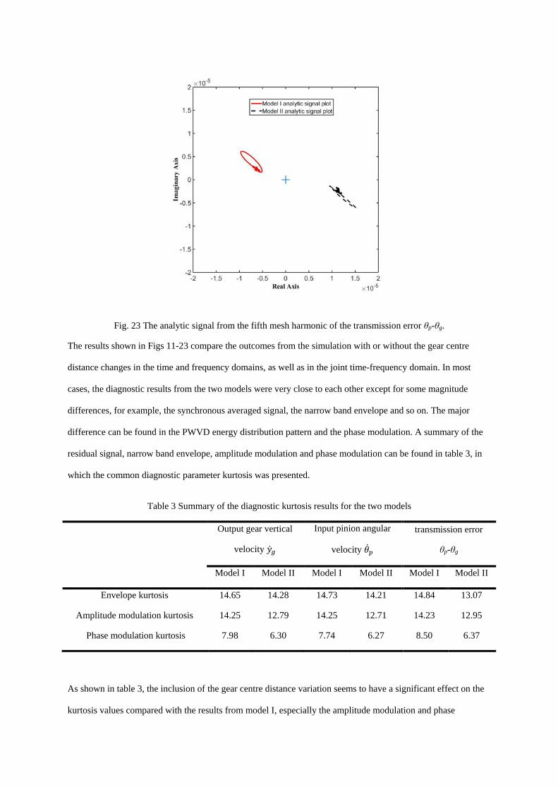
Fig. 23 The analytic signal from the fifth mesh harmonic of the transmission error θp-θg.
The results shown in Figs 11-23 compare the outcomes from the simulation with or without the gear centre
distance changes in the time and frequency domains, as well as in the joint time-frequency domain. In most
cases, the diagnostic results from the two models were very close to each other except for some magnitude
differences, for example, the synchronous averaged signal, the narrow band envelope and so on. The major
difference can be found in the PWVD energy distribution pattern and the phase modulation. A summary of the
residual signal, narrow band envelope, amplitude modulation and phase modulation can be found in table 3, in
which the common diagnostic parameter kurtosis was presented.
Table 3 Summary of the diagnostic kurtosis results for the two models
Output gear vertical
velocity �̇�𝑦𝑔𝑔
Input pinion angular
velocity �̇�𝜃𝑝𝑝
transmission error
θp-θg
Model I Model II Model I Model II Model I Model II