Dynamic Modulus of Hot Mix Asphalt FINAL REPORT Submitted by NJDOT Research Project Manager Dr. Nazhat Aboobaker FHWA-NJ-2009-011 Dr. Thomas Bennert* Senior Research Engineer In cooperation with New Jersey Department of Transportation Bureau of Research and Technology and U.S. Department of Transportation Federal Highway Administration * Dept. of Civil & Environmental Engineering Center for Advanced Infrastructure & Transportation (CAIT) Rutgers, The State University Piscataway, NJ 08854-8014
Transcript
Dynamic Modulus of Hot Mix Asphalt
FINAL REPORT
Submitted by
NJDOT Research Project Manager Dr. Nazhat Aboobaker
FHWA-NJ-2009-011
Dr. Thomas Bennert* Senior Research Engineer
In cooperation with
New Jersey Department of Transportation
Bureau of Research and Technology and
U.S. Department of Transportation Federal Highway Administration
* Dept. of Civil & Environmental Engineering Center for Advanced Infrastructure & Transportation (CAIT)
Rutgers, The State University Piscataway, NJ 08854-8014
Disclaimer Statement
"The contents of this report reflect the views of the author(s) who is (are) responsible for the facts and the
accuracy of the data presented herein. The contents do not necessarily reflect the official views or policies of the New Jersey Department of Transportation or the Federal Highway Administration. This report does not constitute
a standard, specification, or regulation."
The contents of this report reflect the views of the authors, who are responsible for the facts and the accuracy of the
information presented herein. This document is disseminated under the sponsorship of the Department of Transportation, University Transportation Centers Program, in the interest of
information exchange. The U.S. Government assumes no liability for the contents or use thereof.
1. Report No. 2. Government Accession No.
TECHNICAL REPORT STANDARD TITLE PAGE
3. Rec ip ient ’s Cata log No.
5 . Repor t Date
8. Performing Organization Report No.
6. Performing Organizat ion Code
4. Ti t le and Subt i t le
7. Author(s)
9. Performing Organization Name and Address 10. Work Unit No.
11. Contract or Grant No.
13. Type of Report and Period Covered
14. Sponsoring Agency Code
12. Sponsoring Agency Name and Address
15. Supplementary Notes
16. Abstract
17. Key Words
19. Security Classif (of this report)
Form DOT F 1700.7 (8-69)
20. Security Classif. (of this page)
18. Distribution Statement
21. No of Pages 22. Price
June - 2009
CAIT/Rutgers
Final Report 1/2007 – 6/2009
FHWA-NJ-2009-011
New Jersey Department of Transportation CN 600 Trenton, NJ 08625
Federal Highway Administration U.S. Department of Transportation Washington, D.C.
One of the most critical parameters needed for the upcoming Mechanistic Empirical Pavement Design Guide (MEPDG) is the dynamic modulus (E*), which will be used for flexible pavement design. The dynamic modulus represents the stiffness of the asphalt material when tested in a compressive-type, repeated load test. The dynamic modulus is one of the key parameters used to evaluate both rutting and fatigue cracking distresses in the MEPDG. The computer software that accompanies the MEPDG also provides general default parameters for the dynamic modulus (i.e. – Level 2 and 3 inputs). However, caution has already been issued by the National Cooperative Highway Research Program (NCHRP) researchers as to the appropriateness of these parameters for regional areas. The major concern is that state agencies will use these default values blindly and sacrifice accuracy of the design. Hence, making the new mechanistic procedure no better than using a structural number (SN) with the old AASHTO method. There were three primary objectives of the research study. First, the current version of the dynamic modulus test, AASHTO TP62-07, was evaluated to determine the relative precision of the test method, and if required, recommend a modified procedure with better precision. The second objective of the study was to develop a dynamic modulus catalog for use with the Mechanistic Empirical Pavement Design Guide (MEPDG) by testing plant-produced and laboratory-compacted samples of various asphalt mixtures. This would supercede Level 2 inputs currently in the MEPDG for New Jersey. The third primary objective of the research study was to assess the accuracy of two commonly utilized dynamic modulus prediction equations; 1) Witczak Prediction Equation and 2) Hirsch Model. The database developed during the study also led to the development of correlations between dynamic modulus and fatigue cracking and rutting performance of asphalt mixtures.
TABLE OF CONTENTS Page # ABSTRACT 1 OBJECTIVE 2 PHASE 1 - PRECISION OF DYNAMIC MODULUS 2
Testing Program 3 HMA Mixture Design and Material Preparation 5 Analysis of Test Results 5
Bulk Specific Gravity of Test Specimens 5 Dynamic Modulus Test Results 6
PRECISION STATEMENT ASSESSMENT 10 Analysis of Variance 12 Development of Precision Statements for AASHTO TP62-07 15 Influence on MEPDG Distress Predictions 16 Reduction in Test Temperature Data 18
PHASE 2 – DYNAMIC MODULUS CATALOG DEVELOPMENT 20 Data Analysis 21
RESULTS OF DYNAMIC MODULUS CATALOG 24 Asphalt Binder Inputs 25 Dynamic Modulus Test Results 27 Low Temperature Test Results 29
PHASE 4 - DYNAMIC MODULUS VS ASPHALT MIXTURE PERFORMANCE 36 Dynamic Modulus and Rutting Resistance 36 Dynamic Modulus and Fatigue Cracking 44
CONCLUSIONS AND RECOMMENDATIONS 53 Conclusions – Precision of the Dynamic Modulus Test 53 Conclusions – Evaluation of Prediction Equations 55 Conclusions – Development of Proposed Performance Criteria Using the Dynamic Modulus Test 55 Recommendations – Precision of the Dynamic Modulus Test 56 Recommendations – Evaluation of Prediction Equations 56 Recommendations – Use of the Dynamic Modulus Catalog 57 Recommendations – Use of Dynamic Modulus for Performance Indicator 57
REFERENCES 58 APPENDIX 61
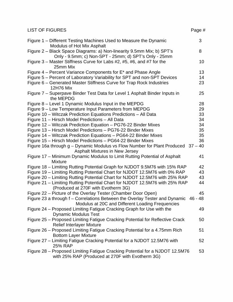
LIST OF FIGURES Page # Figure 1 – Different Testing Machines Used to Measure the Dynamic 3 Modulus of Hot Mix Asphalt Figure 2 – Black Space Diagrams: a) Non-linearity 9.5mm Mix; b) SPT’s 8 Only - 9.5mm; c) Non-SPT - 25mm; d) SPT’s Only - 25mm Figure 3 – Master Stiffness Curve for Labs #2, #5, #6, and #7 for the 10
25mm Mix Figure 4 – Percent Variance Components for E* and Phase Angle 13 Figure 5 – Percent of Laboratory Variability for SPT and non-SPT Devices 14 Figure 6 – Generated Master Stiffness Curve for Trap Rock Industries 23 12H76 Mix Figure 7 – Superpave Binder Test Data for Level 1 Asphalt Binder Inputs in 25 the MEPDG Figure 8 – Level 1 Dynamic Modulus Input in the MEPDG 28 Figure 9 – Low Temperature Input Parameters from MEPDG 29 Figure 10 – Witczak Prediction Equations Predictions – All Data 33 Figure 11 – Hirsch Model Predictions – All Data 34 Figure 12 – Witczak Prediction Equation – PG76-22 Binder Mixes 34 Figure 13 – Hirsch Model Predictions – PG76-22 Binder Mixes 35 Figure 14 – Witczak Prediction Equations – PG64-22 Binder Mixes 35 Figure 15 – Hirsch Model Predictions – PG64-22 Binder Mixes 36 Figure 16a through g – Dynamic Modulus vs Flow Number for Plant Produced 37 – 40 Asphalt Mixtures in New Jersey Figure 17 – Minimum Dynamic Modulus to Limit Rutting Potential of Asphalt 41 Mixture Figure 18 – Limiting Rutting Potential Graph for NJDOT 9.5M76 with 15% RAP 42 Figure 19 – Limiting Rutting Potential Chart for NJDOT 12.5M76 with 0% RAP 43 Figure 20 – Limiting Rutting Potential Chart for NJDOT 12.5M76 with 25% RAP 43 Figure 21 – Limiting Rutting Potential Chart for NJDOT 12.5M76 with 25% RAP 44 (Produced at 270F with Evotherm 3G) Figure 22 – Picture of the Overlay Tester (Chamber Door Open) 45 Figure 23 a through f – Correlations Between the Overlay Tester and Dynamic 46 - 48 Modulus at 20C and Different Loading Frequencies Figure 24 – Proposed Limiting Fatigue Cracking Graph for Use with the 49 Dynamic Modulus Test Figure 25 – Proposed Limiting Fatigue Cracking Potential for Reflective Crack 50 Relief Interlayer Mixture Figure 26 – Proposed Limiting Fatigue Cracking Potential for a 4.75mm Rich 51 Bottom Layer Mixture Figure 27 – Limiting Fatigue Cracking Potential for a NJDOT 12.5M76 with 52 25% RAP Figure 28 – Proposed Limiting Fatigue Cracking Potential for a NJDOT 12.5M76 53 with 25% RAP (Produced at 270F with Evotherm 3G)
ii
LIST OF TABLES Page # Table 1 – Test Equipment and Accessories Used by Different Laboratories 4 Table 2 – Mixture Design Properties Used for Dynamic Modulus Test 5 Specimens Table 3 – Average and Range of Micro-strain Level for Four Different 9 Laboratories for the 25mm Mix Table 4 – Precision Statement Generated for AASHTO TP62-07 and 16 Potential Modifications Table 5 – MEPDG Predicted Pavement Distresses for Different Dynamic 18 Modulus Testing/Analysis Schemes Table 6 - NCHRP Report 614 Recommended Testing Temperatures and 20 Loading Frequencies Table 7 – Example of Resultant Dynamic Modulus Values from Reduced Testing 24 Procedure Table 7 – Conventional Binder Test Results for Level 1 Inputs 26 Table 8 – Superpave Binder Tests for Level 1 Inputs 27 Table 9 – NJDOT Level 1 Low Temperature Cracking Input Parameters for the 30 MEPDG Table 10 - Minimum Flow Number Requirements (adapted from NCHRP 35 Project 9-33) Table 11 – Minimum Required Dynamic Modulus to Limit Rutting Potential of 41 Asphalt Mixtures Table 12 – Dynamic Modulus Performance Bands for Limiting Fatigue Cracking 49 Potential
1
ABSTRACT One of the most critical parameters needed for the Mechanistic Empirical Pavement Design Guide (MEPDG) is the dynamic modulus (E*), which is used for flexible pavement design. The dynamic modulus represents the stiffness of the asphalt material when tested in a compressive-type, repeated load test. The dynamic modulus is one of the key parameters used to evaluate both rutting and fatigue cracking distress predictions in the MEPDG. The computer software that will accompany the MEPDG provides general default parameters for the dynamic modulus. However, caution has already been issued by the National Cooperative Highway Research Program (NCHRP) researchers as to the appropriateness of these parameters for regional areas. The major concern is that state agencies will use these default values blindly and sacrifice accuracy of the design. Hence, making the new mechanistic procedure no better than using a structural number (SN) with the old AASHTO method. To ensure that the New Jersey Department of Transportation (NJDOT) will be prepared for the upcoming design procedure, a research project was conducted to evaluate the dynamic modulus test and parameters. The research project encompassed evaluating the dynamic modulus of approximately twenty different hot mix asphalt mixtures that are currently approved by the NJDOT. The dynamic modulus (E*) values for each mixture evaluated is represented using a technique called a master stiffness curve. The E* master stiffness curve is a single curve that represents the asphalt materials’ stiffness relationship to loading frequency and temperature. This procedure is called Level I for the MEPDG and will provide the most accurate distress predictions during design. The measured E* values were also compared to that of the Witczak predictive equation and the Hirsch model. The Witczak predictive equation has been selected by the NCHRP researchers for the Level II and III design in the MEPDG. However, many researchers feel that perhaps the Hirsch model provides more accurate results. The Witczak predictive equation is based on the mix gradation, asphalt binder viscosity properties, and volumetric properties of the hot mix asphalt, while the Hirsch model is based on the asphalt binder stiffness (G*) and the voids in mineral aggregate (VMA) and voids filled with asphalt (VFA). The accuracy of the predictive equations was compared to the measured laboratory results of the NJ Dynamic Modulus Catalog and recommendations regarding their appropriateness provided. Another important aspect of the research project was the development of a “precision-type statement” for use by the NJDOT regarding the current dynamic modulus test protocol (AASHTO TP62-07). Currently, a precision statement does not exist regarding multiple laboratories. Eight laboratories were contacted and asked to participate in a round robin study regarding the dynamic modulus test. All laboratories are, or were at one time, AMRL accredited for hot mix asphalt. The precision assessment provided valuable information regarding the expected precision the NJDOT can expect if dynamic modulus testing is to be conducted by different laboratories and test equipment. Based on the precision testing, a modified dynamic modulus testing procedure was recommended to increase the general precision of the test results.
2
During the development of the Dynamic Modulus catalog, repeated load and Overlay Tester tests were conducted on the identical mixtures. Correlations were developed between the dynamic modulus and rutting (Flow Number – repeated load) and fatigue cracking (Overlay Tester) tests. The correlations allow the use of the dynamic modulus test for to test for rutting and fatigue cracking prone asphalt mixtures. OBJECTIVE There were three primary objectives of the research study. First, the current version of the dynamic modulus test, AASHTO TP62-07, was evaluated to determine the relative precision of the test method, and if required, recommend a modified procedure with better precision. The second objective of the study was to develop a dynamic modulus catalog for use with the Mechanistic Empirical Pavement Design Guide (MEPDG) by testing plant-produced and laboratory-compacted samples of various asphalt mixtures. The third primary objective of the research study was to assess the accuracy of two commonly utilized dynamic modulus prediction equations; 1) Witczak Prediction Equation and 2) Hirsch Model. The database developed during the study also led to the development of correlations between dynamic modulus and fatigue cracking and rutting performance of asphalt mixtures. The fatigue cracking comparisons were generated using the Overlay Tester and field performance criteria developed by the Texas Department of Transportation (TxDOT). The rutting comparisons were generated using the Flow Number parameter and field performance criteria developed during the NCHRP 9-33, A Mix Design Method for Hot Mix Asphalt (HMA). PHASE 1 - PRECISION OF DYNAMIC MODULUS With the development and release of the Mechanistic Empirical Pavement Design Guide, MEPDG (1), greater emphasis has been placed on hot mix asphalt (HMA) characterization, in particular, the modulus or stiffness properties. The MEPDG uses HMA stiffness for various environmental conditions, traffic speeds, etc., to calculate pavement strains which are then used to predict pavement distresses. Currently, AASHTO TP62-07, Standard Method of Test for Determining Dynamic Modulus of Hot-Mix Asphalt (2) is recommended to determine the stiffness properties (Dynamic Modulus or Complex Modulus, E*) of HMA. The dynamic modulus can be measured on most servo-hydraulic testing machines capable of producing a controlled, sinusoidal (haversine) compressive load. The testing machine should have the capability of applying a load over a range of frequencies from 0.1 to 25 Hz and stress level up to 2800 kPa (400 psi). For sinusoidal loads, the standard error of the applied load shall be less than 5% (2). An environmental chamber is also required to condition the test specimens at different temperatures. The environmental chamber shall be capable of controlling the temperature of the specimen over a temperature range from –10 to 60°C (14 to 140°F) to an accuracy of ± 0.5°C (1°F). Figure 1 shows some of the different types of testing machines utilized for measuring dynamic modulus of HMA specimens.
3
Figure 1 – Different Testing Machines Used to Measure the Dynamic Modulus of Hot Mix Asphalt
With the dynamic modulus being one of the prime material inputs required for flexible pavement design/evaluation in the MEPDG, numerous researchers have explored the various factors affecting the dynamic modulus properties, which include aggregate gradation, asphalt binder stiffness, and mixture volumetrics (3, 4, 5, 6, 7). These studies have also led to different methodologies to predict the dynamic modulus based on these material properties (8, 9, 10, 11, 12, 13). However, none of the studies to date have evaluated the precision of the AASHTO TP62 test method when different laboratories test the same material, nor have they investigated how the precision, or variability among the different laboratories, would affect the predicted distresses of the MEPDG. Testing Program A Round Robin testing program was undertaken to assess the testing variability associated with AASHTO TP62-07, Standard Method of Test for Determining Dynamic Modulus of Hot-Mix Asphalt (HMA). The Round Robin testing program consisted of seven (7) different laboratories having the capability of adequately performing AASHTO TP62-07. The laboratories included:
• Advanced Asphalt Technologies (AAT), Sterling, VA.; • Burns, Cooley, Dennis, Inc. (BCD), Jackson, MS.; • National Center for Asphalt Technology (NCAT) at Auburn University, AL; • North Central Superpave Center at Purdue University (Purdue), IN; • Rutgers Asphalt Pavement Laboratory at Rutgers University (RAPL), NJ; • Texas Transportation Institute (TTI) at Texas A&M University, TX; and • Pavement Research Institute of Southeastern Massachusetts at the University of
Massachusetts (UMass) Dartmouth, MA.
4
The Round Robin testing program was designed to test two different HMA, Superpave-designed HMA mixtures; 9.5mm and 25mm nominal maximum aggregate size (NMAS). Each laboratory was asked to conduct the latest version of AASHTO TP62 on three specimens of each mixture designation (total of six test samples) and to report all results in accordance with AASHTO TP62-07. The collected test data were then evaluated in a precision statement environment, where ASTM E691 was used to evaluate the variability of the test procedure. Three of the seven laboratories used a Simple Performance Tester (SPT) machine for testing, which possesses some operational characteristics that deviate slightly from the details in AASHTO TP62-07 Standard Method of Test for Determining Dynamic Modulus of Hot-Mix Asphalt (HMA). The main differences are discussed by Bonaquist (14) and are summarized below:
to 54.4oC; • SPT Micro-strain Range: 75 to 125; AASHTO TP62-07 specifies 50 to 150; • No rest periods in-between cycles in SPT; AASHTO TP62-07, Section 11.8
recommends typical rest periods of two minutes; and • SPT: 10 preconditioning cycles followed by 10 loading cycles; AASHTO TP62-
07 specifies a greater number of preconditioning cycles according to Table 6 of AASHTO TP62-07.
Although the above does mention some differences between the SPT test machines and other test machines conforming to AASHTO TP62-07, both seem to be interchangeable and widely acceptable with respect to measuring the dynamic modulus properties of hot mix asphalt. A complete summary of equipment, including gyratory compactors, test machines and accessories used by the different laboratories in this study is shown in Table 1.
Table 1 – Test Equipment and Accessories Used by Different Laboratories
HMA Mixture Design and Material Preparation Two Superpave HMA mixtures, described in Table 2, were designed at the Rutgers University Asphalt Pavement Laboratory (RAPL). Both mixtures contained New Jersey trap rock (diabase) aggregate materials, PG64-22 asphalt binder, and were designed at 100 design gyrations. Loose mix was produced and packaged for each test specimen. A quality control assessment was made for every fifth sample, including washed gradations and maximum specific gravity (Gmm), performed in accordance with AASHTO specifications. Each participating laboratory received four (4) sealed, wax-lined boxes of loose mix for each mixture designation, with each box containing 7,400 ± 5 grams of mix. Each box was assigned a sample ID number, and the samples were randomly assigned to the seven (7) different laboratories, thereby minimizing any bias that may have occurred during sample production. In addition to the samples, each participating laboratory received a letter including specific instructions on mixture conditioning, gyratory compaction, sample preparation, testing, and data recording. The laboratories were instructed to use three (3) of the samples for AASHTO TP62-07 testing, and the fourth sample for other necessary activities (i.e. – internal temperature probe, load level selection, etc.).
Analysis of Test Results Bulk Specific Gravity of Test Specimens Prior to conducting AASHTO TP62-07, the laboratories determined the bulk specific gravity, Gmb, in accordance with AASHTO T166 for each test specimen after coring and cutting. The variability of the samples is important to consider because the AASHTO
Table 2 – Mixture Design Properties Used for Dynamic Modulus Test Specimens
TP62-07 procedure includes specimen preparation. Thus, any variability in specimen preparation is included in the variability of the dynamic modulus test method. According to AASHTO T 166, “duplicate specific gravity results by the same operator should not be considered suspect unless they differ by more than 0.02.” Four specimens fell just outside that range; one 9.5mm and three 25mm samples. Final statistics for all test specimens were as follows:
• 9.5mm Mix: Average Gmb = 2.548 g/cm3; Standard Deviation = 0.017 g/cm3; Coefficient of Variation (COV) = 0.663%; Average Air Voids = 5.73%
• 25mm Mix: Average Gmb = 2.599 g/cm3; Standard Deviation = 0.014 g/cm3; Coefficient of Variation (COV) = 0.523%; Average Air Voids = 5.76%
Review of the AASHTO Material Reference Laboratory (AMRL) Proficiency Sample results for the 2007 Gyratory Samples shows that out of 498 laboratories, the average standard deviation of the bulk specific gravity, as determined by AASHTO T166, was 0.0271 g/cm3 with an average Coefficient of Variation of 1.04%. Therefore, even though four of the dynamic modulus test specimens fell out of compliance with AASHTO T166, the precision results were within expectations. A review of each laboratories specimen dimensional data showed that the average standard deviation in specimen height was 0.26mm and the average standard deviation in specimen diameter was 0.077mm. Dynamic Modulus Test Results
A cursory review of the dynamic modulus data was performed by evaluating the COV for various data groupings. When assessing the test results for each laboratory for all temperatures and loading frequencies, the coefficient of variation (COV) ranged from 7.7 percent to 43.5 percent, with an average COV of 25.7 percent. Lesser variation was attained at intermediate test temperatures and faster loading frequencies. When evaluating only the laboratories that used a Simple Performance Tester (SPT), the average COV decreased slightly to 23.1%. The general precision of the within-laboratory results (each lab separately), as determined by the COV, were much better. The average COV for the test results for all labs was 11.2%, with the average COV of the laboratories using the SPT units being 10.9%. The within-laboratory COV reported is in agreement with data reported elsewhere (5, 15). The test results suggested that there were differences between the measured dynamic modulus values of identical mixtures when prepared and tested in accordance with AASHTO TP62-07 by the different laboratories. A more detailed look at the test data was conducted to try and locate the reasons for the discrepancies. Black Space Diagram In an attempt to identify testing variability and/or non-linearity in the material behavior due to non-compliance to the recommended micro-strain levels, the dynamic modulus and phase angle were averaged for each laboratory’s data and plotted in Black Space
7
(16, 17). Figure 2a, b, c, and d contain the Black Space plots for the different mixes and laboratories. The Black Space diagrams for Lab #1 and #2 indicate that either nonlinearity or measurement error was occurring at the intermediate to higher test temperatures for the 9.5mm mix. Intermediate and higher test temperatures are represented towards the middle and left side of the curves, respectively. This is compared to the Black Space plots of the three Simple Performance Test (SPT) devices (Labs #3, #4, and #6) where the curves attained excellent R2 values and appeared close to one another, especially Labs #3 and #6. Similar discrepancies can be seen for the 25mm mixes in Figure 2c and 2d, where Figure 2c shows the Black Space diagram for the non-SPT machines, and Figure 2d shows the Black Space diagram for the SPT machines. It should be noted that Labs #5 and #7 in Figure 2c do show good uniformity in their respective Black Space diagrams, as noted with their R2 values being greater than 0.94. Unfortunately, the curves are shifted away from one another indicating discrepancies in the measured dynamic modulus and phase angle values.
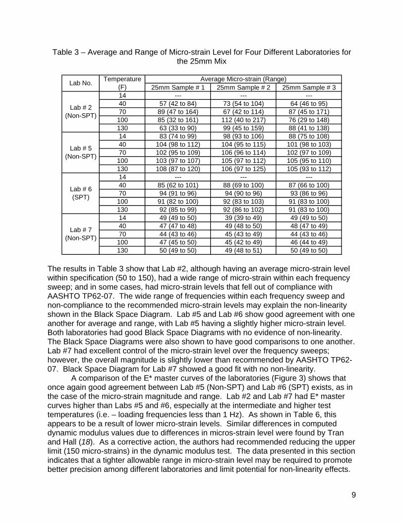
Since the Black Space diagrams had shown potential issues with non-linearity, a closer look at the magnitude of micro-strain levels was conducted. For the laboratories using the SPT test machines, the micro-strain levels averaged 80 to 110 μ-strains. Lab #2, which showed non-linearity in the Black Space Diagram, had micro-strain levels that averaged between 70 and 90 μ-strains. However, the range of strain level during each frequency sweep (all frequencies tested at a constant temperature) was wide. For example, Table 3 shows the average, minimum and maximum micro-strain levels for the frequency sweeps for four different laboratories for the 25mm mix; 1) SPT Machine (Lab #6), 2) Non-SPT with good micro-strain control (Lab #5); 3) Non-SPT with poor micro-strain control (Lab #2), and 4) Non-SPT with good micro-strain control, but low micro-strain levels (Lab #7).
8
R2 = 0.8239
R2 = 0.8584
0
5
10
15
20
25
30
35
40
45
3 3.5 4 4.5 5 5.5 6 6.5 7Log E* (psi)
Phas
e A
ngle
(deg
rees
)Lab # 1
Lab # 2
R2 = 0.9828
R2 = 0.9813
R2 = 0.9918
0
5
10
15
20
25
30
35
40
45
3 3.5 4 4.5 5 5.5 6 6.5 7Log E* (psi)
Phas
e A
ngle
(deg
rees
)
Lab # 3
Lab # 4
Lab # 6
(a) (b)
R2 = 0.8961R2 = 0.9457
R2 = 0.9938
R2 = 0.9852
0
5
10
15
20
25
30
35
40
45
3 3.5 4 4.5 5 5.5 6 6.5 7Log E* (psi)
Phas
e A
ngle
(deg
rees
)
Lab # 1
Lab # 2
Lab # 5
Lab # 7
R2 = 0.984
R2 = 0.9903
R2 = 0.987
0
5
10
15
20
25
30
35
40
45
3 3.5 4 4.5 5 5.5 6 6.5 7Log E* (psi)
Phas
e A
ngle
(deg
rees
)
Lab # 3
Lab # 4
Lab # 6
(b) (d)
Figure 2 – Black Space Diagrams: a) Non-linearity 9.5mm Mix; b) SPT’s Only - 9.5mm; c) Non-SPT - 25mm; d) SPT’s Only - 25mm
9
Table 3 – Average and Range of Micro-strain Level for Four Different Laboratories for the 25mm Mix
25mm Sample # 1 25mm Sample # 2 25mm Sample # 314 --- --- ---40 57 (42 to 84) 73 (54 to 104) 64 (46 to 95)70 89 (47 to 164) 67 (42 to 114) 87 (45 to 171)100 85 (32 to 161) 112 (40 to 217) 76 (29 to 148)130 63 (33 to 90) 99 (45 to 159) 88 (41 to 138)14 83 (74 to 99) 98 (93 to 106) 88 (75 to 108)40 104 (98 to 112) 104 (95 to 115) 101 (98 to 103)70 102 (95 to 109) 106 (96 to 114) 102 (97 to 109)100 103 (97 to 107) 105 (97 to 112) 105 (95 to 110)130 108 (87 to 120) 106 (97 to 125) 105 (93 to 112)14 --- --- ---40 85 (62 to 101) 88 (69 to 100) 87 (66 to 100)70 94 (91 to 96) 94 (90 to 96) 93 (86 to 96)100 91 (82 to 100) 92 (83 to 103) 91 (83 to 100)130 92 (85 to 99) 92 (86 to 102) 91 (83 to 100)14 49 (49 to 50) 39 (39 to 49) 49 (49 to 50)40 47 (47 to 48) 49 (48 to 50) 48 (47 to 49)70 44 (43 to 46) 45 (43 to 49) 44 (43 to 46)100 47 (45 to 50) 45 (42 to 49) 46 (44 to 49)130 50 (49 to 50) 49 (48 to 51) 50 (49 to 50)
Lab # 5 (Non-SPT)
Lab # 6 (SPT)
Lab # 7 (Non-SPT)
Lab No. Temperature (F)
Average Micro-strain (Range)
Lab # 2 (Non-SPT)
The results in Table 3 show that Lab #2, although having an average micro-strain level within specification (50 to 150), had a wide range of micro-strain within each frequency sweep; and in some cases, had micro-strain levels that fell out of compliance with AASHTO TP62-07. The wide range of frequencies within each frequency sweep and non-compliance to the recommended micro-strain levels may explain the non-linearity shown in the Black Space Diagram. Lab #5 and Lab #6 show good agreement with one another for average and range, with Lab #5 having a slightly higher micro-strain level. Both laboratories had good Black Space Diagrams with no evidence of non-linearity. The Black Space Diagrams were also shown to have good comparisons to one another. Lab #7 had excellent control of the micro-strain level over the frequency sweeps; however, the overall magnitude is slightly lower than recommended by AASHTO TP62-07. Black Space Diagram for Lab #7 showed a good fit with no non-linearity.
A comparison of the E* master curves of the laboratories (Figure 3) shows that once again good agreement between Lab #5 (Non-SPT) and Lab #6 (SPT) exists, as in the case of the micro-strain magnitude and range. Lab #2 and Lab #7 had E* master curves higher than Labs #5 and #6, especially at the intermediate and higher test temperatures (i.e. – loading frequencies less than 1 Hz). As shown in Table 6, this appears to be a result of lower micro-strain levels. Similar differences in computed dynamic modulus values due to differences in micros-strain level were found by Tran and Hall (18). As a corrective action, the authors had recommended reducing the upper limit (150 micro-strains) in the dynamic modulus test. The data presented in this section indicates that a tighter allowable range in micro-strain level may be required to promote better precision among different laboratories and limit potential for non-linearity effects.
10
1,000
10,000
100,000
1,000,000
10,000,000
0.000001 0.0001 0.01 1 100 10000 1000000
Loading Frequency (Hz)
Dyn
amic
Mod
ulus
, E* (
psi)
Lab #2Lab #5 Lab #6Lab #7
Figure 3 – Master Stiffness Curve for Labs #2, #5, #6, and #7 for the 25mm Mix
PRECISION STATEMENT ASSESSMENT When considering the precision of a test method, significant sources of variability must be identified and expressed in terms of repeatability and reproducibility. The accepted practice for determining the precision of a test method is given in ASTM E 691, “Standard Practice for Conducting an Interlaboratory Study to Determine the Precision of a Test Method” (19). This practice recommends that an interlaboratory study include a minimum of 6 laboratories and 3 materials, and that each laboratory perform triplicate testing. In this study, only 2 materials were included. It is noted, however, that each dynamic modulus test provides two responses (E* and phase angle) for each combination of five testing temperatures and six frequencies, resulting in a total of 60 responses for each sample tested.
In the ASTM E 691 procedure, within-laboratory (k) and between-laboratory (h) consistency statistics are computed in order to determine whether there were laboratories that generated data that was not typical of the overall experiment. Inconsistencies are then noted and investigated, and if a valid reason exists, extreme data points may be removed from the dataset. Although several of the h and k statistics slightly exceeded the critical values, all exceptions were considered to be borderline. Thus, no results were removed from the dataset.
For the data generated in this portion of the study, the following observations were noted with respect to E*:
11
• At 14 degrees F, Lab #7 produced positive h-statistics for E*, while the other 3 labs provided primarily negative statistics. The Lab #7 values were close to, but did not exceed, critical values. This trend was consistent for all testing frequencies.
• At 40 and 70 degrees F, Lab #2 appeared to provide E* values that were most distant from the other laboratories, exceeding the critical h-statistic for the 25.0mm mixture tested at mid-range frequencies.
• At 100 and 130 degrees F, Lab #4 was most variable for the mid-range testing frequencies, exceeding the critical h-statistic for both materials at the 100F / 1 Hz testing combination.
• At the 40F and 70F testing temperatures, Lab #2 generated the greatest within-laboratory variability. In general, the variability was most pronounced for the 9.5mm mixture.
• At 100F, Lab #4 generally exhibited the greatest variability, having the greatest k-statistic values at lower testing frequencies.
• At 130F, Lab #2 and Lab #3 displayed the greatest overall levels of variability, such that variability for Lab #2 decreased as frequency increased, and the variability for Lab #3 increased as frequency increased.
With respect to phase angle, the following trends were observed: • At 14 F, Lab #1 produced positive h-statistics, while those for the other labs were
primarily negative. Results were most variable for the 25Hz / 25.0mm mixture testing combination.
• At 40F, the Lab #2 and Lab #1 results appeared to exhibit the greatest deviation from the group (i.e., greatest h-statistics), especially at the low and intermediate testing frequencies.
• At 70F, the Lab #1 h-statistics were higher than those for the other labs for all testing frequencies except 25 Hz. Most statistics for this laboratory were near the critical value.
• At 100F, the Lab #7 results displayed the greatest deviation from the group, especially at the low and intermediate frequencies.
• At 130F, all laboratories displayed somewhat greater levels of variability, but were generally similar for all testing frequencies.
• At 14F, Lab #1 exhibited the greatest within-laboratory variability, which was more pronounced for the 9.5mm mixture.
• At 40F, Lab #1 exceeded the critical within-laboratory variability, primarily at the higher testing frequencies. Lab #3 displayed excessive variability for the 25.0mm mix at the 0.5Hz testing frequency.
• At 70F, Lab #2 had the greatest within-laboratory variability, having k statistic values near or above critical for the intermediate and high frequencies. Excessive variability was also detected for this laboratory at the 100F / 1Hz / 9.5mm testing combination.
• At 130F, the within-laboratory variability for Lab #3 and Lab #5 generally decreased as testing frequency increased, while that for Lab #2 appeared to increase as frequency increased.
12
From the within-laboratory and between-laboratory statistics, precision statistics for repeatability and reproducibility relative to E* and phase angle were calculated for each material, temperature, and frequency combination. In general, the greatest amounts of variability were detected for the 14F and 130F testing temperatures. Variability appeared to be less affected by testing frequency, although variability in phase angle was slightly greater at lower frequencies. Analysis of Variance In order to further investigate the components of variance present in the dataset, the E* data was evaluated using an analysis of variance with two random effects. In essence, the total variability of the E* test was calculated according to
where is the total variability, is the variance component for materials, is the variance component for laboratories, represents the interaction between materials and laboratories, and is the random experimental error. The repeatability of the method is described by , and the reproducibility of the method is represented by the sum of and because it includes the additional variability in the test method generated by various laboratories. For the dynamic modulus test, the variability between laboratories includes both the variation in the processes used in sample preparation and the devices used to measure dynamic modulus.
For each combination of temperature and frequency, the variance components associated with E* were estimated. In cases where the interaction between parts and operators was not statistically significant, this term was omitted from the model, and only the variance due to materials and laboratories were estimated.
In general, the experimental variance (i.e., repeatability) was relatively low, and the largest proportion of error was attributed to the laboratory error, or reproducibility term. This is reasonable because the reproducibility variance contains the largest number of sources of variability. Material variability was also larger than the pure experimental error, which means that the intentional variability in the data created through the use of different materials was readily detected by the dynamic modulus test.
Overall, it was apparent that the measurement of E* was more variable at low temperatures. This trend was noted for the experimental, repeatability, and reproducibility error terms. However, the magnitude of the E* measurements was also greater at low temperatures. Thus, the variability associated with each testing temperature was relatively proportional to the measured value of E*. Similar trends were noted for phase angle, such that the larger values for variance existed for the larger measures of phase angle. The greatest variability associated with phase angle was attributed to the laboratory variance at lower frequencies, and was much more pronounced for the 130F testing temperature. Interestingly, within each temperature category, E* variability increased as testing frequency increased, but phase angle variability decreased as testing frequency increased.
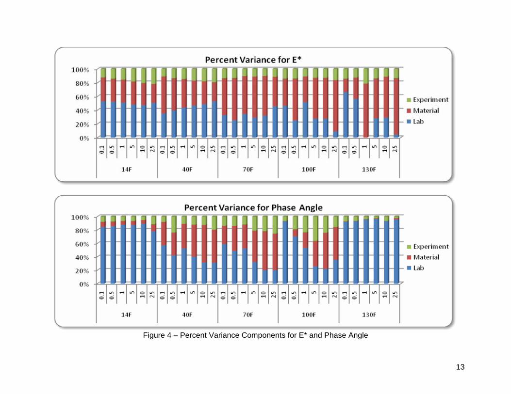
In order to provide a fairer comparison of repeatability and reproducibility across the range of temperatures, variance components were next considered as a percentage
13
Figure 4 – Percent Variance Components for E* and Phase Angle
14
Figure 5 – Percent of Laboratory Variability for SPT and non-SPT Devices
15
of total variance, . These comparisons are given in Figure 4. Although less pronounced, the percent variability comparisons confirm that the laboratory component of variance for E* is most variable at the lowest testing temperature, while the precision of phase angle is detrimentally affected by both the lowest and highest test temperatures. Thus, the greatest between-laboratory precision of the dynamic modulus test is attained at the intermediate temperatures (40F, 70F, and 100F). Because slight differences were known to exist between various types of dynamic modulus testing equipment, an analysis of variance (ANOVA) was used to investigate the effect of the various equipment types. The results of the analysis indicated that the SPT and non-SPT devices provided statistically significant differences in measures of both E* and phase angle. In order to assess the impact of this difference on the precision of the dynamic modulus test, a similar comparison of variance components was completed separately for the SPT and non-SPT devices, as shown in Figure 5. Again, the greatest precision was achieved at intermediate test temperatures, with the SPT devices exhibiting much less variability between laboratories than the non-SPT devices. Thus, if the 14F and 130F testing temperatures were removed, the precision of the dynamic modulus test could be significantly improved. It has previously been suggested that the number of temperature and testing frequencies be reduced for routine dynamic modulus testing (11, 20). In addition, not all E* testing equipment is capable of testing at the 14F temperature. Thus, eliminating the 14F testing temperature would improve the variability of the E* testing measurements, and eliminating the 130F test temperature would be beneficial for improving the reproducibility of phase angle measurements. Development of Precision Statements for AASHTO TP62-07 A Precision Statement was generated for AASHTO TP62-07 (2) in accordance with ASTM E691 (19). The Precision Statement utilized the recorded dynamic modulus (E*) and phase angle data for each laboratory and each material, at each test temperature and loading frequency. The results of the Precision Statement are shown in Table 4. Because the variance components were not constant for varying levels of temperature and frequency, precision statistics are presented as percentages. The Precision Statement for AASHTO TP62-07, for all test devices, shows better repeatability for phase angle measurements than for the calculated dynamic modulus, especially for the Single Operator Precision. A relatively high variability is shown for Multi-Laboratory Precision when evaluating the acceptable range of 2 results, called D2S%. The generated Precision Statement for AASHTO TP62-07 reinforces the variability in test results previously described in Figures 4. In an attempt to evaluate the potential increase in precision, a Precision Statement was again generated for all test devices, but with the elimination of the low and high test temperatures, which were previously identified as having the highest level of variability in the test data. By eliminating the low and high test temperatures, a slight increase in the overall precision was determined. However, the level of the D2S% still indicates a relatively high level of variability exists. Since the elimination of low and high temperatures only slightly increased the precision of AASHTO TP62-07, further Precision Statements were generated by separating the different test equipment into two groups; 1) SPT devices only and 2)
16
Non-SPT Devices only and eliminating the low and high test temperatures. The previous results shown as Figures 4 and 5 indicated that the highest level of variability was associated with the low and high test temperatures, and that Non-SPT devices incurred greater variability than the SPT devices. As shown previously in Figure 5, the Percent of Laboratory Variability was lower for all comparable test temperatures and loading frequencies for the SPT devices when compared to the Non-SPT devices when the low and high test temperatures are eliminated. Similar to the results in Figure 5, the SPT devices resulted in a better precision statement than the Non-SPT devices.
Table 4 – Precision Statement Generated for AASHTO TP62-07 and Potential Modifications
- 1S% = Coefficient of Variation- D2S% = Acceptable Range of 2 Results- Low Temperature = 14oF- High Temperature = 130oF
SPT Devices Only, Eliminating High and Low Temperatures
Single Operator Precision
Multi-Laboratory Precision
Non-SPT Devices Only, Eliminating High and Low Temperatures
Single Operator Precision
Multi-Laboratory Precision
All Test Devices, All Temperatures
Single Operator Precision
Multi-Laboratory Precision
All Test Devices, Eliminating High and Low Temperatures
Single Operator Precision
Multi-Laboratory Precision
Influence on MEPDG Distress Predictions To evaluate how the precision of AASHTO TP62-07 influences the distress predictions of the MEPDG, a theoretical pavement section was designed. The pavement section, and its respective constituent materials, is shown below:
The Average Annual Daily Truck Traffic (AADTT) used in the analysis was 10,000. The remaining traffic inputs were left as the MEPDG Default values. Indirect Tensile and Creep Compliance testing, AASHTO T322 (21), were conducted at -10oC (14oF) to provide Level 2 HMA input parameters for the Thermal Cracking model. Each laboratory’s dynamic modulus test results were used as Level 1 inputs, along with Conventional Level 1 asphalt binder properties. Air voids and VMA were computed for each individual lab based on the reported bulk specific gravity (Gmb), as well as the effective binder content, average maximum specific gravity (Gmm) and average bulk specific gravity of the aggregate blend (Gsb) determined during the Quality Control testing.
The MEPDG requires that the dynamic modulus measured at -10oC (14oF) and 54.4oC (130oF) test temperatures be used as input values to construct the master stiffness curve. However, as discussed earlier, the some laboratories were not capable of measuring the dynamic modulus at test temperatures lower than 0oC. Therefore, for those laboratories, the Limiting Maximum Modulus methodology proposed by Bonaquist and Christensen (20) was used to generate dynamic modulus parameters at the -10oC (14oF) test temperature for the master curve construction. Analyses conducted by Bonaquist and Christensen (20) had shown that this approach had a minimal effect on the generated master stiffness curves, and therefore should minimally affect the predicted pavement distresses. Three MEPDG predicted pavement distresses were selected for comparison; HMA Rutting (inches), Longitudinal Cracking (ft/mile), and % Alligator Cracking in Wheelpath. The test results are shown in Table 5. Overall, the MEPDG analysis showed;
• A minimal change (from maximum to minimum) was found in the HMA Rutting due to the precision of the dynamic modulus test results (0.33 inches to 0.44 inches);
• An significant change (from maximum to minimum) was found in the Longitudinal Cracking results due to the precision of the dynamic modulus test results (24.3 to 215 ft/mile); and
• A minimal change (from maximum to minimum) was found in the % Alligator Cracking due to the precision of the dynamic modulus test results (3.7 to 5.2% of Wheelpath).
As discussed earlier, the precision analysis showed that the variability in the
dynamic modulus test results were highest at the low and high test temperatures, as well as the 25 Hz test frequency. Therefore, repeated MEPDG runs were conducted by modifying these parameters in an attempt to increase the precision of the MEPDG distress predictions.
18
Table 5 – MEPDG Predicted Pavement Distresses for Different Dynamic Modulus Testing/Analysis Schemes
Actual Test Data 0.44 195 5.2Low Temp Hirsch 0.43 161 5.5
Low and High Temp Hirsch 0.42 157 5.5Actual Test Data 0.33 24.3 3.7Low Temp Hirsch 0.33 24.3 3.7
Low and High Temp Hirsch 0.34 37.7 3.9Actual Test Data 0.42 124 5.1Low Temp Hirsch 0.42 124 5.1
Low and High Temp Hirsch 0.42 136 5.3Actual Test Data 0.37 58.7 4.6Low Temp Hirsch 0.37 58.7 4.6
Low and High Temp Hirsch 0.38 92.3 4.9Actual Test Data 0.43 215 5.2Low Temp Hirsch 0.43 177 5.6
Low and High Temp Hirsch 0.42 157 5.6Actual Test Data 0.43 155 4.5Low Temp Hirsch 0.42 122 5
Low and High Temp Hirsch 0.41 115 5.1Actual Test Data 0.39 94.6 3.9Low Temp Hirsch 0.37 61.7 4.4
Low and High Temp Hirsch 0.39 97.6 4.7
E* Testing Scheme Rutting (inches)
Long. Cr. (ft/mile)
Allig. Cr. (% of Wheelpath)
Lab # 5
Lab # 6
Lab # 7
Lab #
Lab # 1
Lab # 2
Lab # 3
Lab # 4
Reduction in Test Temperature Data As shown in the precision analysis, the dynamic modulus data had the largest variability at the low and high test temperatures. Work conducted under the NCHRP 9-29 Project, Simple Performance Test, has recommended that the low test temperature (14oF) can be eliminated from the testing scheme and substituted with predicted modulus values of the Hirsch model for the master stiffness curve construction. NCHRP 9-29 is also recommending eliminating the 130oF test temperature for high test temperatures based on the high temperature PG Grade (i.e. – PG64-22 would use 95oF and PG76-22 would use 113oF).
Two additional runs in the MEPDG were conducted with 1) actual test values at 10oC (14oF) replaced by Hirsch Model estimates, as proposed by Bonaquist and Christensen (2006); and 2) actual test values at both the -10oC (14oF) and 54.4oC (130oF) test temperatures replaced by Hirsch Model estimates to generate the dynamic modulus values. The purpose of eliminating these test temperatures and using the Hirsch predictions was to evaluate how a reduced dynamic modulus testing procedure would affect the MEPDG predicted pavement distresses. The results of the additional MEPDG runs are shown in Table 6. It should be noted that Labs # 2, # 3, and # 4 were not able test at the 14oF test temperature and therefore, the Actual Test Data and Low Temp Hirsch results are identical.
19
For Labs # 1, # 5, # 6, and # 7, using the Hirsch predictions for 14oF in place of the actual test data;
• Resulted in minimal changes in HMA Rutting, reduced the longitudinal cracking by approximately 35 ft/mile, and increased % Alligator Cracking by approximately 0.4%
When both the 14oF (10oC) and 130oF (54.4oC) test temperature data were replaced by the Hirsch Model values, the following observations were made:
• Minimal changes were noted for HMA Rutting; • Longitudinal Cracking predictions varied by laboratory:
o For Labs # 2, # 3, # 4, and # 7, an average increase of 15.5 ft/mile was observed. The actual change ranged between 3 ft/mile and 33.6 ft/mile;
o For Labs # 1, # 5, and # 6, an average decrease of 45.3 ft/mile was observed. The actual change ranged between 38 and 58 ft/mile.
• % Alligator Cracking increased slightly. Therefore, based on the results of the precision statement development, it is recommended that the NJDOT utilize the reduced dynamic modulus test procedure, currently being recommended by Bonaquist and Christensen (20). The test procedure not only provides more precise results when comparing the multiple laboratory test results, but also provides an overall quicker test procedure.
20
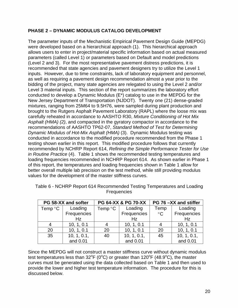
PHASE 2 – DYNAMIC MODULUS CATALOG DEVELOPMENT The parameter inputs of the Mechanistic Empirical Pavement Design Guide (MEPDG) were developed based on a hierarchical approach (1). This hierarchical approach allows users to enter in project/material specific information based on actual measured parameters (called Level 1) or parameters based on Default and model predictions (Level 2 and 3). For the most representative pavement distress predictions, it is recommended that state agencies and pavement designers try to utilize the Level 1 inputs. However, due to time constraints, lack of laboratory equipment and personnel, as well as requiring a pavement design recommendation almost a year prior to the bidding of the project, many state agencies are relegated to using the Level 2 and/or Level 3 material inputs. This section of the report summarizes the laboratory effort conducted to develop a Dynamic Modulus (E*) catalog to use in the MEPDG for the New Jersey Department of Transportation (NJDOT). Twenty one (21) dense-graded mixtures, ranging from 25M64 to 9.5H76, were sampled during plant production and brought to the Rutgers Asphalt Pavement Laboratory (RAPL) where the loose mix was carefully reheated in accordance to AASHTO R30, Mixture Conditioning of Hot Mix Asphalt (HMA) (2), and compacted in the gyratory compactor in accordance to the recommendations of AASHTO TP62-07, Standard Method of Test for Determining Dynamic Modulus of Hot-Mix Asphalt (HMA) (3). Dynamic Modulus testing was conducted in accordance to the modified procedure recommended from the Phase 1 testing shown earlier in this report. This modified procedure follows that currently recommended by NCHRP Report 614, Refining the Simple Performance Tester for Use in Routine Practice (4). Table 1 shows the recommended testing temperatures and loading frequencies recommended in NCHRP Report 614. As shown earlier in Phase 1 of this report, the temperatures and loading frequencies shown in Table 1 allow for better overall multiple lab precision on the test method, while still providing modulus values for the development of the master stiffness curves.
Since the MEPDG will not construct a master stiffness curve without dynamic modulus test temperatures less than 32oF (0oC) or greater than 120oF (48.9oC), the master curves must be generated using the data collected based on Table 1 and then used to provide the lower and higher test temperature information. The procedure for this is discussed below.
21
Data Analysis The general form of the dynamic modulus master curve is a modified version of the dynamic modulus master curve equation included in the Mechanistic Empirical Design Guide (MEDG) (1)
( )re
MaxEωγβ
δδ log1*log
++−
+= (1)
where:
⎮E*⎮ = dynamic modulus, psi ωr = reduced frequency, Hz Max = limiting maximum modulus, psi δ, β, and γ = fitting parameters
The reduce frequency in Equation 1 is computed using the Arrhenius equation (5).
⎟⎟⎠
⎞⎜⎜⎝
⎛−
Δ+=
r
ar TT
E 1114714.19
loglog ωω (2)
where: ωr = reduced frequency at the reference temperature ω = loading frequency at the test temperature Tr = reference temperature, °K T = test temperature, °K ΔEa = activation energy (treated as a fitting parameter)
The final form of the dynamic modulus master curve equation is obtained by substituting Equation 2 into Equation 1.
( )⎪⎭
⎪⎬⎫
⎪⎩
⎪⎨⎧
⎥⎥⎦
⎤
⎢⎢⎣
⎡⎟⎟⎠
⎞⎜⎜⎝
⎛−⎟⎠
⎞⎜⎝
⎛Δ++
+
−+=
r
aTT
E
e
MaxE11
14714.19log
1
*logωγβ
δδ (3)
The shift factors at each temperature are given by Equation 4,
[ ] ⎟⎟⎠
⎞⎜⎜⎝
⎛−
Δ=
r
a
TTE
Ta 1114714.19
)(log (4)
where: a(T) = shift factor at temperature T Tr = reference temperature, °K T = test temperature, °K ΔEa = activation energy (treated as a fitting parameter)
22
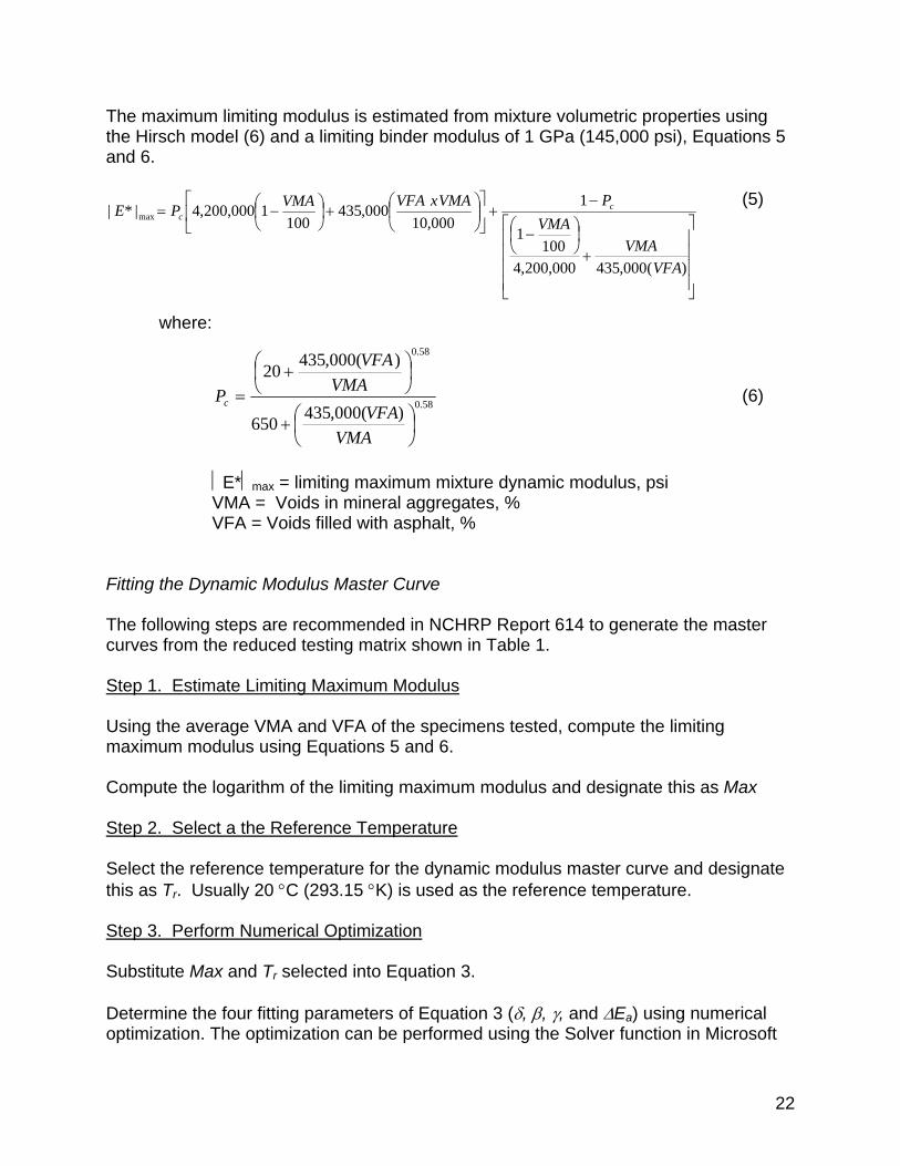
The maximum limiting modulus is estimated from mixture volumetric properties using the Hirsch model (6) and a limiting binder modulus of 1 GPa (145,000 psi), Equations 5 and 6.
⎥⎥⎥⎥
⎦
⎤
⎢⎢⎢⎢
⎣
⎡
+⎟⎠⎞
⎜⎝⎛ −
−+⎥
⎦
⎤⎢⎣
⎡⎟⎠
⎞⎜⎝
⎛+⎟
⎠⎞
⎜⎝⎛ −=
)(000,435000,200,4100
1
1000,10
000,435100
1000,200,4|*| max
VFAVMA
VMAPVMAxVFAVMAPE c
c (5)
where:
58.0
58.0
)(000,435650
)(000,43520
⎟⎠⎞
⎜⎝⎛+
⎟⎠⎞
⎜⎝⎛ +
=
VMAVFA
VMAVFA
Pc (6)
⏐E*⏐max = limiting maximum mixture dynamic modulus, psi VMA = Voids in mineral aggregates, % VFA = Voids filled with asphalt, %
Fitting the Dynamic Modulus Master Curve The following steps are recommended in NCHRP Report 614 to generate the master curves from the reduced testing matrix shown in Table 1. Step 1. Estimate Limiting Maximum Modulus Using the average VMA and VFA of the specimens tested, compute the limiting maximum modulus using Equations 5 and 6. Compute the logarithm of the limiting maximum modulus and designate this as Max Step 2. Select a the Reference Temperature Select the reference temperature for the dynamic modulus master curve and designate this as Tr. Usually 20 °C (293.15 °K) is used as the reference temperature. Step 3. Perform Numerical Optimization Substitute Max and Tr selected into Equation 3. Determine the four fitting parameters of Equation 3 (δ, β, γ, and ΔEa) using numerical optimization. The optimization can be performed using the Solver function in Microsoft
23
EXCEL®. This is done by setting up a spreadsheet to compute the sum of the squared errors between the logarithm of the average measured dynamic moduli at each temperature/frequency combination and the values predicted by Equation 3. The Solver function is used to minimize the sum of the squared errors by varying the fitting parameters in Equation 3. The following initial estimates are recommended: δ = 0.5, β = -1.0, γ =-0.5, and ΔEa = 200,000. An example of this methodology is shown in Figure 6 for a 12H76 asphalt mixture from Trap Rock Industries. As the figure indicates, the reduced testing, shown in Orange, provides adequate information for input into the MEPDG. Then, using the master curve parameters shown in Equation (1), one can shift the curves to determine the respective Dynamic Modulus values at the MEPDG required higher and lower test temperatures. An example of this type of calculation is shown as Table 7.
RESULTS OF DYNAMIC MODULUS CATALOG When utilizing the Level 1 hierarchy in the MEPDG, two sets of information is required to be inputted for flexible pavements; 1) Asphalt binder properties and 2) Dynamic Modulus properties of the mixtures. The low temperature Indirect Tensile Strength and Creep Compliance inputs are only required for the surface course mixture. The low temperature inputs were not required for this research effort. However, four (4) typical surface course mixes were tested under the Level 1 low temperature hierarchy procedure to provide NJDOT with low temperature MEPDG mixture property inputs and are provided in this document for potential use.
25
Asphalt Binder Inputs Two different types of asphalt binder input values can be selected for use as Level 1 hierarchy inputs; 1) Superpave binder test data or 2) Conventional test data. Superpave binder test data refers to shear modulus (G*) and phase angle (δ) collected during the PG binder grading. However, the temperature range required for the MEPDG inputs is a low at 40oF up to almost where the PG grading occurs. Figure 7 shows a screen shot Level 1 inputs required for the asphalt binder properties.
Figure 7 – Superpave Binder Test Data for Level 1 Asphalt Binder Inputs in the MEPDG A similar input page is provided for the conventional binder test data that includes;
o Absolute and kinematic viscosities; o Softening point; o Penetration at different temperatures;
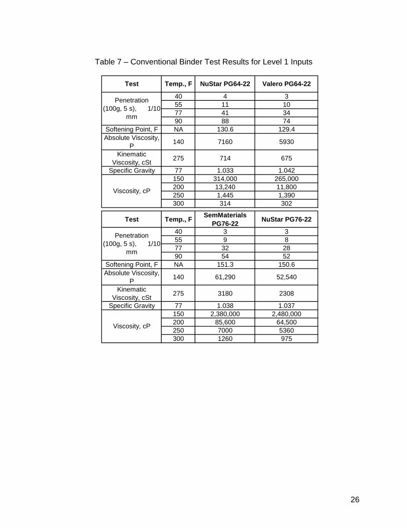
Although not included in the original scope of work, both sets of binder tests (Conventional and Superpave) were conducted for typical PG64-22 and PG76-22 asphalt binders. Test results for the Level 1 Conventional and Superpave Binder Tests are shown in Tables 7 and 8.
26
Table 7 – Conventional Binder Test Results for Level 1 Inputs
40 4 355 11 1077 41 3490 88 74
Softening Point, F NA 130.6 129.4Absolute Viscosity,
Table 8 – Superpave Binder Tests for Level 1 Inputs
G* (Pa) Delta (degrees)Temperature, F Angular Frequency = 10 rad/sec
50 17,600,000 47.371.6 2,506,000 59.9
136.4 581 86.3
93.2 300,700 69.9114.8 4,096 80.8
158 5,504 65.6179.6 1,775 69.0
G* (Pa) Delta (degrees)Temperature, F Angular Frequency = 10 rad/sec
63.4
50 21,070,000 40.071.6 3,570,000 51.2
136.4 18,560 64.0
NuStar PG64-22
SemMaterials PG76-22
93.2 504,600 60.3114.8 83,590
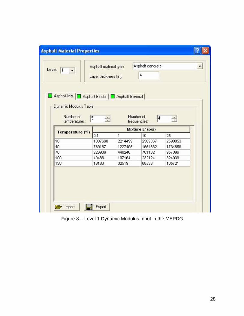
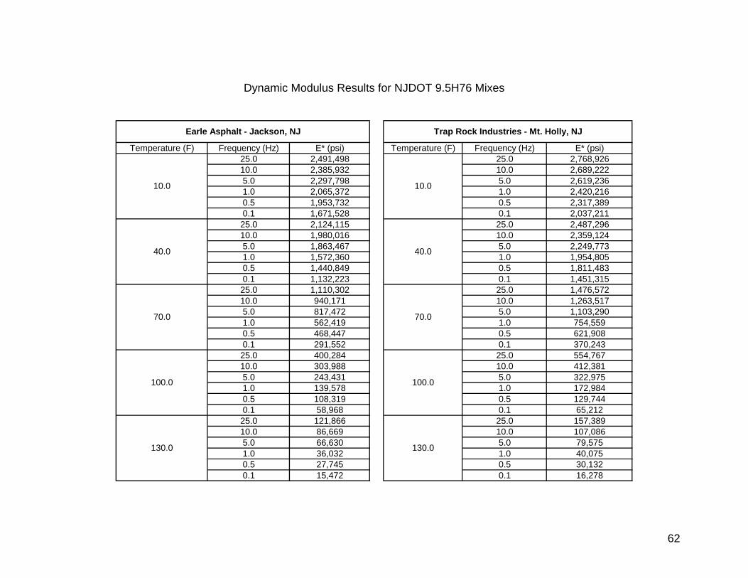
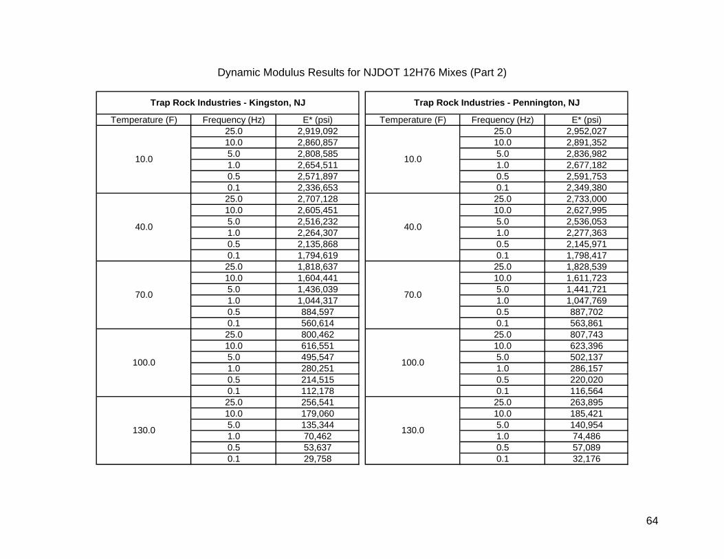
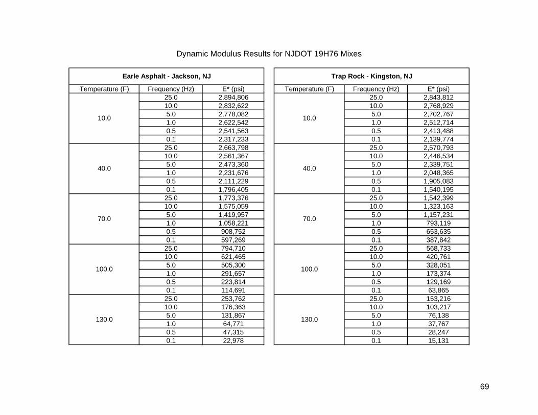
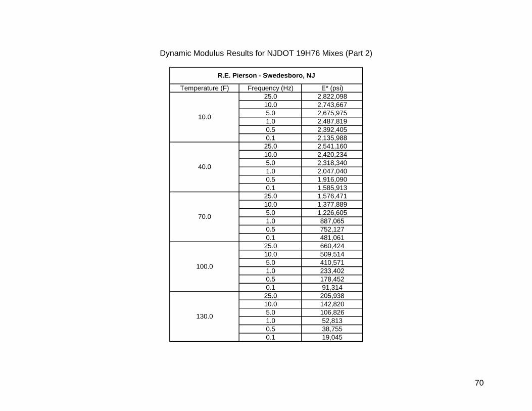
Dynamic Modulus Test Results As discussed earlier, a reduced testing procedure was conducted using the Simple Performance Tester to help increase the precision of the dynamic modulus testing protocol. In doing so, both the low and high temperatures, as specified in AASHTO TP62-07, are eliminated from testing. However, the MEPDG requires test data from both of these temperatures to construct the master stiffness curves in order to predict resultant pavement stress and strain during traffic and environmental loading. In order to provide these inputs, the high and low test temperature data is extrapolated from the resultant master curve of the reduced testing procedure, as discussed and shown earlier, and generated into a format used by the MEPDG, as shown in Figure 8. This process was conducted on thirteen (19) different dense-graded mixes and two (2) stone mastic asphalt mixtures. The test results are shown in the tables located in the Appendix.
28
Figure 8 – Level 1 Dynamic Modulus Input in the MEPDG
29
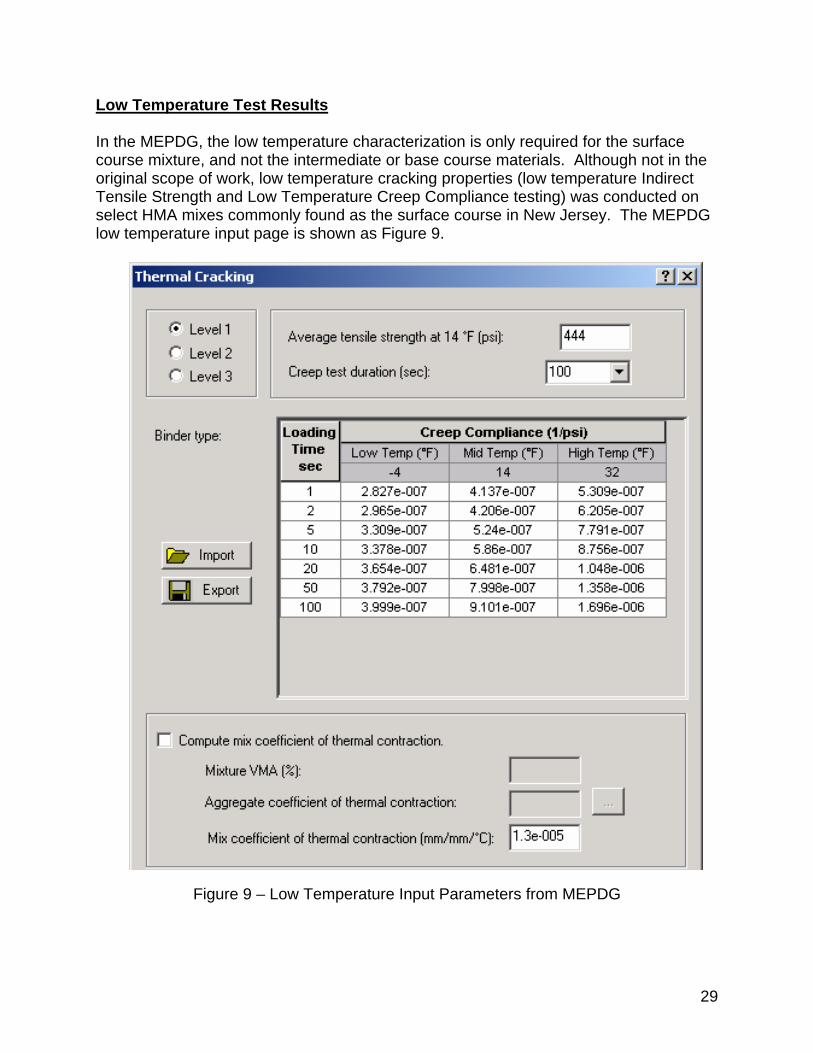
Low Temperature Test Results In the MEPDG, the low temperature characterization is only required for the surface course mixture, and not the intermediate or base course materials. Although not in the original scope of work, low temperature cracking properties (low temperature Indirect Tensile Strength and Low Temperature Creep Compliance testing) was conducted on select HMA mixes commonly found as the surface course in New Jersey. The MEPDG low temperature input page is shown as Figure 9.
Figure 9 – Low Temperature Input Parameters from MEPDG
30
Only four surface course mixtures were used in the low temperature testing and tested in accordance with AASHTO T322, Standard Method of Test for Determining the Creep Compliance and Strength of Hot-Mix Asphalt (HMA) Using the Indirect Tensile Test Device (7). However, since the low temperature performance is typically controlled by the asphalt binder grade and general volumetrics of the mixture, the surface course mixtures shown in the upcoming tables should provide a good estimate of a majority of NJDOT mixture designation’s low temperature characterization. Table 9 – NJDOT Level 1 Low Temperature Cracking Input Parameters for the MEPDG
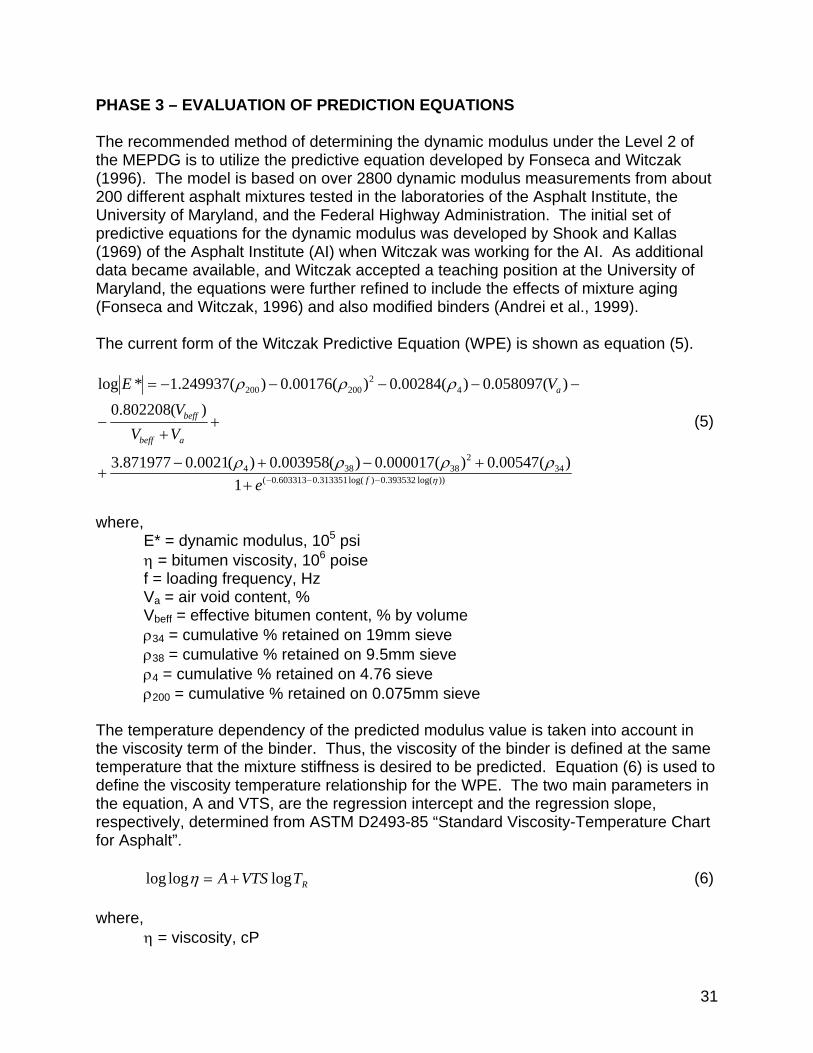
PHASE 3 – EVALUATION OF PREDICTION EQUATIONS The recommended method of determining the dynamic modulus under the Level 2 of the MEPDG is to utilize the predictive equation developed by Fonseca and Witczak (1996). The model is based on over 2800 dynamic modulus measurements from about 200 different asphalt mixtures tested in the laboratories of the Asphalt Institute, the University of Maryland, and the Federal Highway Administration. The initial set of predictive equations for the dynamic modulus was developed by Shook and Kallas (1969) of the Asphalt Institute (AI) when Witczak was working for the AI. As additional data became available, and Witczak accepted a teaching position at the University of Maryland, the equations were further refined to include the effects of mixture aging (Fonseca and Witczak, 1996) and also modified binders (Andrei et al., 1999). The current form of the Witczak Predictive Equation (WPE) is shown as equation (5).
where, E* = dynamic modulus, 105 psi η = bitumen viscosity, 106 poise f = loading frequency, Hz Va = air void content, % Vbeff = effective bitumen content, % by volume ρ34 = cumulative % retained on 19mm sieve ρ38 = cumulative % retained on 9.5mm sieve ρ4 = cumulative % retained on 4.76 sieve ρ200 = cumulative % retained on 0.075mm sieve The temperature dependency of the predicted modulus value is taken into account in the viscosity term of the binder. Thus, the viscosity of the binder is defined at the same temperature that the mixture stiffness is desired to be predicted. Equation (6) is used to define the viscosity temperature relationship for the WPE. The two main parameters in the equation, A and VTS, are the regression intercept and the regression slope, respectively, determined from ASTM D2493-85 “Standard Viscosity-Temperature Chart for Asphalt”. RTVTSA logloglog +=η (6) where, η = viscosity, cP
32
TR = temperature, oRankine A = regression intercept VTS = regression slope (Viscosity Temperature Susceptibility) The original Hirsch model was developed by T.J. Hirsch to calculate the modulus of elasticity of cement concrete or mortar in terms of one empirical constant, the aggregate modulus and cement mastic modulus, and mix proportions. Hirsch assumed that the response of the constituent materials (cement matrix, aggregate, and the composite concrete) behaved in a linear elastic manner. Christensen et al. (2004) developed a relatively simple version of the Hirsch model to predict the dynamic modulus of hot mix asphalt from the complex shear modulus (G*) of the asphalt binder and the volumetric properties of the aggregate mixture (i.e. – voids in mineral aggregate and voids filled with asphalt). The functional form of the Hirsch model prediction equation is shown below.
where,
E* = dynamic modulus of the hot mix asphalt (same temperature and loading frequency as G*) G* = shear modulus of the asphalt binder VMA = voids in mineral aggregate VFA = voids filled with asphalt Prediction Equation Testing Procedure Both the Witczak Prediction Equation and Hirsch Model were compared to the measured dynamic modulus test results for all of the dense graded mixtures tested in the study. The specialty mixes (i.e. – SMA, HPTO, Strata, etc) were not evaluated since the prediction equations were developed only with dense graded mixtures.
33
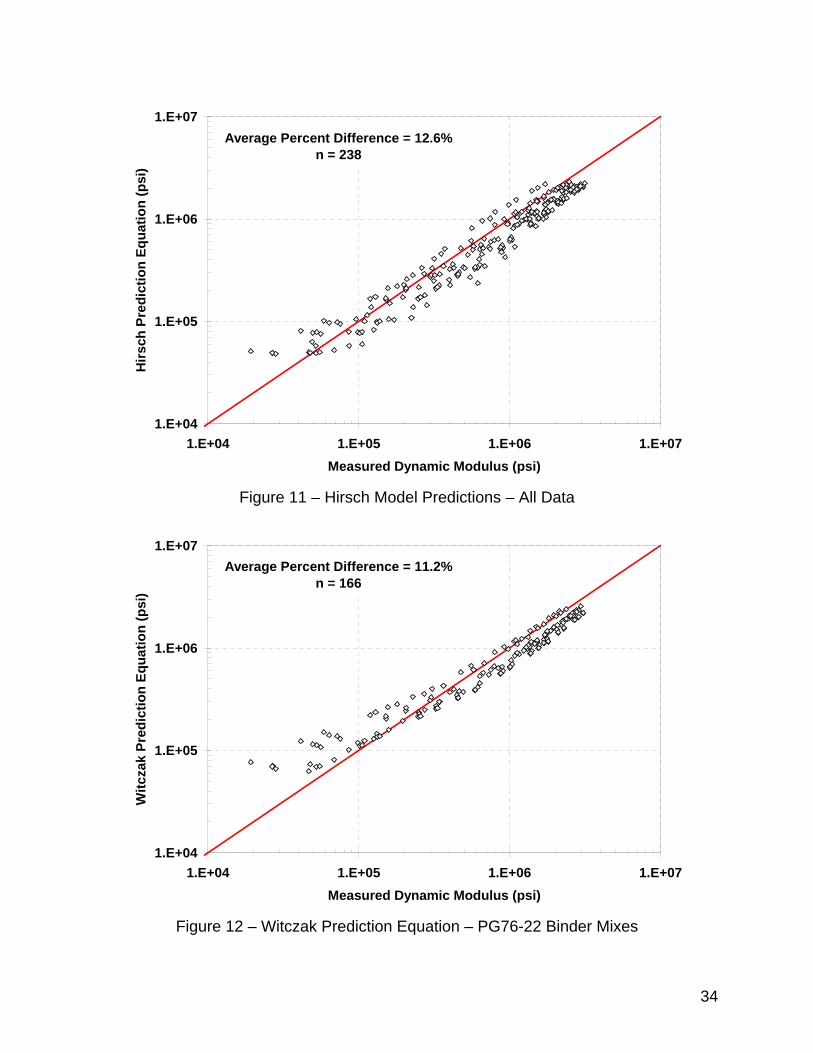
The aggregate and general volumetric properties required in the prediction equations were taken from the HMA Mixture Design Summary Sheet provided to the NJDOT for approval. The asphalt binder properties were measured under RTFO (rolling thin film oven) aging conditions to simulate the aging that occurs during plant production for both PG76-22 and PG64-22 asphalt binders. A total of 238 data points were compared between the measured values and the prediction equations (Witczak Prediction Equation and Hirsch Model). The prediction comparisons of the Witczak Prediction Equation and the Hirsch Model are shown in Figures 10 and 11, respectively. The results indicate that on average, the Witczak Prediction Equation provides a slightly better comparison to the measured dynamic modulus results than the Hirsch Model, 10.5 percent difference and 12.6 percent difference, respectively.
Figure 10 – Witczak Prediction Equations Predictions – All Data
Since it is well accepted that the asphalt binder stiffness plays a significant role in the stiffness of the asphalt mixture, the prediction equations were separated by asphalt binder grade evaluated (Figures 12 through 15). Both prediction equations show better correlations to the PG64-22 asphalt binder than the PG76-22 asphalt binder mixtures. This is logical since most of the datasets used to develop the prediction equations were based on neat asphalt binders.
Figure 15 – Hirsch Model Predictions – PG64-22 Binder Mixes
PHASE 4 - DYNAMIC MODULUS VS ASPHALT MIXTURE PERFORMANCE During the development of the study, sampled loose mix from various paving projects in New Jersey were evaluated under the modified dynamic modulus testing protocol. The sampled mixtures were also evaluated for their rutting susceptibility using the proposed testing protocol developed under NCHRP 9-33, A Mix Design Manual for Hot Mix Asphalt. A database, containing some of the mixtures sampled during this study as well as from other on-going studies, was also developed to evaluate the relationship between fatigue cracking resistance and the dynamic modulus. Dynamic Modulus and Rutting Resistance The relationship between dynamic modulus and rutting resistance was conducted by comparing the dynamic modulus, tested at 45oC, and the Flow Number, measured in the Asphalt Mixture Performance Tester and tested at 54oC. The Flow Number test was performed following the procedures given in NCHRP Report 629, Ruggedness Testing of the Dynamic Modulus and Flow Number Tests with the Simple Performance Tester. An applied deviatoric stress of 600 kPa was used with a test temperature of the average, 7-day maximum pavement temperature 20 mm from the surface, at 50 % reliability as determined using LTPPBind version 3.1 for the location of the original pavement (on average, this equated to 54oC). Table 10 lists minimum values for Flow Number as a function of design traffic level developed during NCHRP 9-33 project.
37
Table 10 - Minimum Flow Number Requirements (adapted from NCHRP Project 9-33)
Traffic Level Million ESALs
Minimum Flow Number
Cycles
Rut Resistance
< 3 < 340 Poor to Fair 3 to < 10 340 Good
10 to < 30 560 Very Good ≥ 30 890 Excellent
Correlations between dynamic modulus, at each test frequency, and Flow Number are shown in Figures 16a through e. The average correlation coefficient (R2) for all frequencies was approximately 0.68, with the best correlation found at the 0.5 Hz.
Figure 16a through g – Dynamic Modulus vs Flow Number for Plant Produced Asphalt
Mixtures in New Jersey
By using the resultant regression equation for each set of data in conjunction with the Flow Number criteria shown in Table 10, minimum dynamic modulus requirements were developed. The minimum dynamic modulus requirements are shown in Table 11 and Figure 17.
41
Table 11 – Minimum Required Dynamic Modulus to Limit Rutting Potential of Asphalt Mixtures
> 30M ESAL's< 30M to > 10M ESAL's< 10M to > 3M ESAL's
E* (ksi) must be above line
Figure 17 – Minimum Dynamic Modulus to Limit Rutting Potential of Asphalt Mixture
To utilize Table 11 and/or Figure 17, dynamic modulus testing is simply conducted on plant-produced mixtures compacted in the laboratory between 6 to 7% air voids at a test temperature of 45oC. The measured dynamic modulus can simply be compared with the requirements of Table 11 or be plotted against the requirements in Figure 17. To meet the traffic level, the dynamic modulus values must be greater than that shown in Table 11 and/or Figure 17.
42
Examples of dynamic modulus results for typical surface course mixtures, and how they would fit into the Limiting Rutting Potential graph are shown in Figures 18 through 21. Figure 18 shows the dynamic modulus results of a NJDOT 9.5M76 with 15% RAP. The test results indicate that this mixture should be sufficient for traffic levels between 10 to 30 millions ESAL’s. However, it should be noted that the “M” mix designated by NJDOT is for traffic levels between 0.3 and 3 million ESAL’s. The graph would suggest that NJDOT’s “M” mix could actually be designed for more asphalt binder and most likely still be able to obtain a traffic level, according to NCHRP Project 9-33, of at least 3 million ESAL’s.
0
50
100
150
200
250
300
350
400
0.01 0.1 1 10 100Loading Frequency (Hz)
Dyn
amic
Mod
ulus
at 4
5C (k
si)
> 30M ESAL's< 30M to > 10M ESAL's< 10M to > 3M ESAL's9.5M76 15% RAP
E* (ksi) must be above line
Figure 18 – Limiting Rutting Potential Graph for NJDOT 9.5M76 with 15% RAP
Figures 19 and 20 show the test results of a 12.5M76 with 0% and 25% RAP, respectively. The results clearly demonstrate the stiffening affect when RAP is included. With 0% RAP, the asphalt mixture would be rated at limiting the rutting potential for traffic levels between 3 to 10 million ESAL’s. Meanwhile, when 25% RAP is incorporated in the same mixture, the asphalt mixture would then be rated at limiting the rutting potential for traffic levels greater than 30 millions ESAL’s.
43
0
50
100
150
200
250
300
350
400
0.01 0.1 1 10 100Loading Frequency (Hz)
Dyn
amic
Mod
ulus
at 4
5C (k
si)
> 30M ESAL's< 30M to > 10M ESAL's< 10M to > 3M ESAL's12M76 0% RAP
E* (ksi) must be above line
Figure 19 – Limiting Rutting Potential Chart for NJDOT 12.5M76 with 0% RAP
0
50
100
150
200
250
300
350
400
0.01 0.1 1 10 100Loading Frequency (Hz)
Dyn
amic
Mod
ulus
at 4
5C (k
si)
> 30M ESAL's< 30M to > 10M ESAL's< 10M to >3M ESAL's12M76 25% RAP
E* (ksi) must be above line
Figure 20 – Limiting Rutting Potential Chart for NJDOT 12.5M76 with 25% RAP
44
Figure 21 shows the results from a different asphalt supplier where the warm mix additive, Evotherm 3G, was used with a production temperature of 270F. Based on the Limiting Rutting Potential graph, the mixture would appear to be rated for a traffic level of approximately 3 million ESAL’s.
0
50
100
150
200
250
300
350
400
0.01 0.1 1 10 100Loading Frequency (Hz)
Dyn
amic
Mod
ulus
at 4
5C (k
si)
> 30M ESAL's
< 30M to > 10M ESAL's
< 10M to > 3M ESAL's
12.5M76 25% RAP (WMA @ 270F)
E* (ksi) must be above line
Figure 21 – Limiting Rutting Potential Chart for NJDOT 12.5M76 with 25% RAP
(Produced at 270F with Evotherm 3G) Dynamic Modulus and Fatigue Cracking Similar to the Limiting Rutting Potential graphs, a Limiting Fatigue Cracking Potential graph was developed for use with dynamic modulus test data. To establish dynamic modulus limits, comparisons were made using the Overlay Tester and established criteria developed by the Texas Department of Transportation (TxDOT). The Overlay Tester is a relatively new test method developed by the Texas Transportation Institute, TTI. The test device simulates the expansion and contraction movements that occur in the joint/crack vicinity of PCC pavements. The test procedure is a fatigue-type test that has shown excellent correlations to fatigue cracking on flexible pavements, as well as reflective cracking on composite pavements (Figure 22).
45
Figure 22 – Picture of the Overlay Tester (Chamber Door Open)
Sample preparation and test parameters used in this study followed that of TxDOT Tex-248-F testing specifications. These include:
o 25oC (77oF) test temperature; o Opening width of 0.025 inches; o Cycle time of 10 seconds (5 seconds loading, 5 seconds unloading); and o Specimen failure defined as 93% reduction in Initial Load.
Twenty four different mixes, consisting of different nominal aggregate sizes, asphalt binder grades, and asphalt binder contents were used to develop a relationship between the fatigue cracking performance in the Overlay Tester and the dynamic modulus. During the initial analysis, both the 4.4oC (39.9oF) and 20oC (68oF) dynamic modulus test data were compared to the Overlay Tester results. Since a better correlation was found at the 20oC dynamic modulus test temperature, this data was used for the development of the Limiting Fatigue Cracking Potential graph. The correlations between the Overlay Tester fatigue cracking and the dynamic modulus at 20C and different loading frequencies are shown in Figures 23a through f. The graphs indicate a relatively good correlation exists between the dynamic modulus and the fatigue cracking resistance of the various NJDOT asphalt mixtures.
Based on the relationships developed in Figures 23a through f, recommendations were made to establish dynamic modulus values to aid in limiting cracking potential (Table 12 and Figure 24). The primary criteria used to establish these performance bands are based on the current TxDOT Overlay Tester criteria, shown below;
o Minimum 300 Cycles for general cracking resistance (primarily surface course mixtures)
46
o Minimum 750 Cycles for immediately overlaying concrete/composite pavements Table 16 and Figure 23 also include performance bands for 200 and 100 cycles in the Overlay Tester, respectively. This was simply included for possible future revisions to the proposed performance bands recommended in this report.
20C, 25 Hz R2 = 0.71
1
10
100
1000
10000
100000
0 200 400 600 800 1000 1200 1400 1600 1800 2000
E* (ksi)
Ove
rlay
Test
er (C
ycle
s)
(a)
20C, 10 Hz R2 = 0.74
1
10
100
1000
10000
100000
0 250 500 750 1000 1250 1500 1750
E* (ksi)
Ove
rlay
Test
er (c
ycle
s)
(b)
47
20C, 5 Hz R2 = 0.76
1
10
100
1000
10000
100000
0 250 500 750 1000 1250 1500
E* (ksi)
Ove
rlay
Test
er (c
ycle
s)
(c)
20C, 1 Hz R2 = 0.81
1
10
100
1000
10000
100000
0 200 400 600 800 1000 1200
E* (ksi)
Ove
rlay
Test
er (c
ycle
s)
(d)
48
20C, 0.5 Hz R2 = 0.82
1
10
100
1000
10000
100000
0 100 200 300 400 500 600 700 800 900 1000
E* (ksi)
Ove
rlay
Test
er (c
ycle
s)
(e)
20C, 0.1 Hz R2 = 0.85
1
10
100
1000
10000
0 100 200 300 400 500 600 700 800
E* (ksi)
Ove
rlay
Test
er (c
ycle
s)
(f)
Figure 23 a through f – Correlations Between the Overlay Tester and Dynamic Modulus at 20C and Different Loading Frequencies
Figure 24 – Proposed Limiting Fatigue Cracking Graph for Use with the Dynamic
Modulus Test
50
To utilize Table 12 and/or Figure 24, dynamic modulus testing is simply conducted on plant-produced mixtures compacted in the laboratory between 6 to 7% air voids at a test temperature of 20oC. The measured dynamic modulus can be compared with the requirements of Table 16 or be plotted against the requirements in Figure 23. To meet the fatigue application level (i.e. – general pavements = minimum of 300 cycles; PCC/composite pavement overlays = minimum of 750 cycles), the dynamic modulus values must be less than that shown in Table 12 and/or Figure 24. Examples of typical NJDOT asphalt mixtures and how they would compare in the proposed Limiting Fatigue Cracking Potential graph is shown in the upcoming figures. Figure 25 shows the dynamic modulus results of a reflective crack relief interlayer (Strata) that was used on Rt 202 during the NJDOT Flexible Overlays for Rigid Pavements study. Figure 25 clearly shows the dynamic modulus of the Strata mixture is well below the 750 cycles line, and therefore, should provide excellent fatigue cracking resistance for PCC/composite overlays.
0
200
400
600
800
1000
1200
1400
0.01 0.1 1 10 100Loading Frequency (Hz)
Dyn
amic
Mod
ulus
at 2
0C (k
si)
750 Cycles in Overlay Tester300 Cycles in Overlay Tester200 Cycles in Overlay Tester100 Cycles in Overlay TesterStrata (Rt 202)
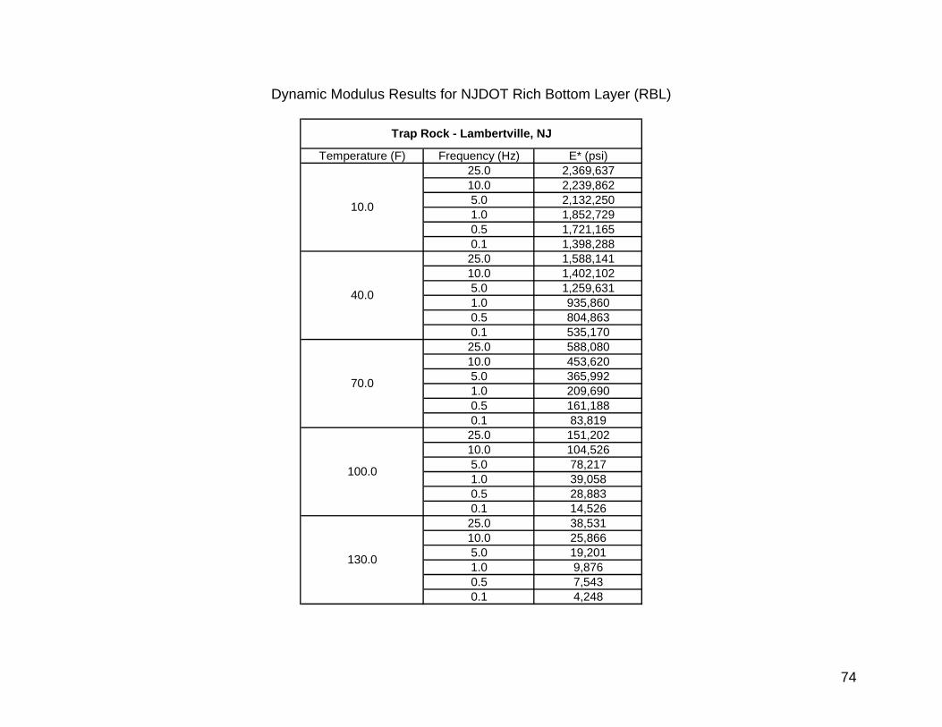
Figure 26 shows the results of a NJDOT 4.75mm Rich Bottom Layer (RBL) asphalt mixture, which was utilized to overlay a PCC pavement on Rt 29. The RBL mixture plots below the 750 cycle line, although not as far below as the Reflective Crack Relief Interlayer. However, the RBL mixture would be classified as an asphalt mixture that would be recommended for placement over PCC/composite pavements to help reduce reflective cracking potential.
0
200
400
600
800
1000
1200
1400
1600
0.01 0.1 1 10 100Loading Frequency (Hz)
Dyn
amic
Mod
ulus
at 2
0C (k
si)
750 Cycles in Overlay Tester300 Cycles in Overlay Tester200 Cycles in Overlay Tester100 Cycles in Overlay Tester4.75mm Rich Bottom Layer
E* (ksi) must be below line
Figure 26 – Proposed Limiting Fatigue Cracking Potential for a 4.75mm Rich Bottom
Layer Mixture Figure 27 shows the results of a NJDOT 12.5M76 with 25% RAP. The test results clearly indicate the excessive stiffness of the mixture and would rate the asphalt mixture as one that would be prone to fatigue cracking.
52
0
200
400
600
800
1000
1200
1400
1600
0.01 0.1 1 10 100Loading Frequency (Hz)
Dyn
amic
Mod
ulus
at 2
0C (k
si)
750 Cycles in Overlay Tester300 Cycles in Overlay Tester200 Cycles in Overlay Tester100 Cycles in Overlay Tester12.5M76 + 25% RAP
E* (ksi) must be below line
Figure 27 – Limiting Fatigue Cracking Potential for a NJDOT 12.5M76 with 25% RAP
Figure 28 shows the test results of a NJDOT 12.5M76 with 25% RAP that was produced using the Evotherm 3G warm mix additive at 270F. It should be noted that the asphalt mixtures in Figure 26 and 27 are from different asphalt suppliers. The test results in Figure 28 indicate that the use of the warm mix technology, and dropping the production temperatures, helped to increase the fatigue resistance. Unfortunately, the fatigue cracking potential is still higher than what would be desired by the NJDOT.
53
0
200
400
600
800
1000
1200
1400
1600
0.01 0.1 1 10 100Loading Frequency (Hz)
Dyn
amic
Mod
ulus
at 2
0C (k
si)
750 Cycles in Overlay Tester300 Cycles in Overlay Tester200 Cycles in Overlay Tester100 Cycles in Overlay Tester12.5M76 + 25% RAP (WMA@270F)
E* (ksi) must be below line
Figure 28 – Proposed Limiting Fatigue Cracking Potential for a NJDOT 12.5M76 with
25% RAP (Produced at 270F with Evotherm 3G) CONCLUSIONS AND RECOMMENDATIONS The study evaluated the dynamic modulus properties of various asphalt mixtures currently approved by the New Jersey Department of Transportation (NJDOT). The study first evaluated the general precision of AASHTO TP62-07, Standard Method of Test for Determining Dynamic Modulus of Hot-Mix Asphalt and provided recommendations on how to improve the precision of the test procedure (shown in Phase 1). Once a modified test procedure was in-place, a dynamic modulus catalog was developed for use with the Mechanistic Empirical Pavement Design Guide (Phase 2). During the catalog’s development, the Witczak Prediction Equation and the Hirsch Model were evaluated and compared with the measured dynamic modulus properties (Phase 3). The mixtures collected and tested during this study also were used to generate a performance-criteria (rutting and fatigue cracking) solely based on the dynamic modulus properties of the asphalt mixtures. Based on the work conducted during this study, the following conclusions and recommendations can be drawn: Conclusions – Precision of the Dynamic Modulus Test A research study was conducted to assess the general precision of AASHTO TP62-07 through a Round Robin-type study. Loose mix was prepared and provided to seven
54
different laboratories that were asked to prepare and test the specimens in accordance with AASHTO TP62-07. The test data was then evaluated in a precision statement environment, as well as in the Mechanistic Empirical Pavement Design Guide software. Based these analyses, the following conclusions were drawn:
• Not all laboratories were capable of testing HMA mixtures at the 14oF test temperature in AASHTO TP62-07. Since the MEPDG currently requires the 14oF test temperature for the generation of the master stiffness curve, a procedure such as the reduced testing procedure recommended by Bonaquist and Christensen (2006) would be required.
• The variability of the dynamic modulus (E*) was greatest at the low testing temperatures with over 50% of the variance being associated with the laboratory itself. Since some labs are currently not capable of testing at 14oF and those that did showed the highest level of variance, the elimination of this test temperature should be considered.
• The variability of phase angle (φ) was greatest at the low and high testing temperatures. This may have been due to non-linearity or micro-strain values falling outside of the recommended range of 50 to 150 micro-strains.
• The use of a Black Space diagram may help to pre-screen test data to ensure non-linearity in the testing did not occur. As shown in this study, laboratories whose Black Space diagrams showed non-linearity had micro-strain values with a relatively high range within a given test temperature.
• The proportion of variance associated with multiple laboratories was significantly larger for non-SPT devices than for SPT devices. Therefore, laboratories considering the future purchase of dynamic modulus test equipment may want to consider procuring a test machine capable of adhering to the specifications of the SPT units. However, it should be noted that only one manufacturer’s SPT machine was involved in the study. This may have attributed to the better precision of the test data.
• A Precision Statement was generated for AASHTO TP62-07 utilizing the test data for all laboratories at all test temperatures and loading frequencies. The Precision Statement indicated that:
o For Single Operator: Dynamic Modulus: 1S% = 13.03; D2S% = 36.47 Phase Angle: 1S% = 6.76; D2S% = 18.93
• Additional Precision Statements were generated for other testing scenarios, including an abridged test procedure that eliminated the low and high test temperatures and also by separating the SPT and Non-SPT devices. The results indicated that the use of the SPT devices with the elimination of the low and high test temperatures produced the best precision characteristics.
• The outputs from the MEPDG pavement distress predictions showed minimal differences in HMA Rutting and % Alligator Cracking between the different laboratories, while large differences in Longitudinal Cracking had occurred for the pavement section evaluated. This may mean that some pavement distresses in
55
the MEPDG are insensitive to dynamic modulus variations from different laboratories, while others are more sensitive. State agencies should recognize this prior to model calibration.
Conclusions – Evaluation of Prediction Equations
o Overall, the Witczak Prediction Equation provided a better comparison to the measured dynamic modulus values than the Hirsch Model. The average percent difference found with the Witczak Prediction Equation was 10.5%, compared to 12.6% percent difference of the Hirsch model.
o The comparisons of the predicted dynamic modulus values were found to be better for the PG64-22 asphalt binders than for the polymer modified PG76-22 asphalt binders. This may have been expected as the original dynamic modulus datasets used to develop the prediction equations primarily consisted of unmodified (neat) asphalt binders, such as the PG64-22 asphalt binder in this study.
o The use of rolling thin film oven (RTFO) aged asphalt binders resulted in reasonable predicted dynamic modulus values for both the Witczak Prediction Equation and the Hirsch Model. This indicates that RTFO aged asphalt binders result in aging that compares favorably to the aging that occurs during plant production of the hot mix asphalt mixtures.
Conclusions – Development of Proposed Performance Criteria Using the Dynamic Modulus Test The database of asphalt mixture performance was correlated to the measured dynamic modulus results for the asphalt mixtures evaluated in this study, as well as the database developed by Rutgers University of the past two years. For permanent deformation (i.e. – rutting), the dynamic modulus was correlated to the Flow Number, measured in the Asphalt Mixture Performance Tester (AMPT). The proposed Flow Number vs Allowable ESAL’s, developed during the NCHRP 9-33 research project, was used to establish dynamic modulus guidelines to limit permanent deformation potential. For the fatigue cracking, the dynamic modulus was correlated to the fatigue cracking results of the Overlay Tester. Overlay Tester criteria, currently implemented by the Texas Department of Transportation (TxDOT), were used to establish dynamic modulus guidelines to limit fatigue cracking potential. The research showed that relatively good correlations were found between the dynamic modulus and the permanent deformation and fatigue cracking properties of the asphalt mixtures. Overall, the Flow Number and Dynamic Modulus properties had an average correlation coefficient (R2) of 0.68, when eliminating the 0.01 Hz dynamic modulus test results. Using the correlations developed for each loading frequency, recommended dynamic modulus “bands” were generated for different ESAL levels, shown as Table 11 and Figure 17.
56
For the fatigue cracking potential, an average correlation coefficient (R2) of 0.78 was found between the Dynamic Modulus and Overlay Tester results. Using the correlations developed, dynamic modulus “bands” were generated and shown in Table 12 and Figure 24. The performance bands recommend maximum dynamic modulus values for generally “good” fatigue resistance of asphalt mixtures, as well as required fatigue performance for placement over PCC/composite pavements (i.e. – mixtures like Reflective Crack Relief Interlayers, Rich Bottom Layer, High Performance Thin Overlays) as indicated by field comparisons at TxDOT. Recommendations – Precision of the Dynamic Modulus Test For use in the MEPDG, it is recommended that the 14oF (-10oC) test temperature be eliminated from the testing scheme of AASHTO TP62-07. Not only did three of the seven laboratories not have the capabilities of testing at this temperature, the dynamic modulus results at the 14oF showed the highest variance among the five test temperatures. For the pavement scenario utilized in this study, this resulted in a reduction of approximately 35 ft/mile for the Longitudinal Cracking and produced minimal changes in HMA Rutting and % Alligator Cracking. Further evaluation of limiting or eliminating the 130oF (54.4oC) test temperature should be conducted. In this study, the 130oF test temperature produced the second highest degree of variation among the five test temperatures specified in AASHTO TP62-07. The phase angle measured at the 130oF test temperature showed the highest level of laboratory variance, meaning the majority of the error involved in the phase angle test data can be attributed to the laboratory testing equipment. This may have been due to error in the applied load waveform or non-linearity associated with testing outside of the linear-elastic range of the material. This was further validated by evaluating the Black Space diagrams of the different laboratories. To ensure the master stiffness curves are constructed properly, a 0.01 Hz loading frequency can be added to the 100oF (37.8oC) test temperature, similar to that recommended by Bonaquist and Christensen (20). Allowable micro-strain ranges in AASHTO TP62-07 should be reduced to a range of 75 to 125 micro-strains, as currently recommended in the NCHRP 9-29 project. The general test results of the different laboratories whose micro-strain levels were within this range showed better agreement. Recommendations – Evaluation of Prediction Equations Both the Witczak Prediction Equation and the Hirsch Model can be used with confidence to provide reasonable estimates of the dynamic modulus for use in the Mechanistic Empirical Pavement Design Guide (MEPDG). However, caution should be taken when using more heavily modified asphalt binders. As shown with the PG76-22 asphalt binders, the percent difference increases when the asphalt binders are polymer-modified. Therefore, it is recommended that the prediction equations not be used for the more heavily modified asphalt binders (i.e. – reflective cracking relief interlayer, bridge deck wearing course, etc.).
57
Recommendations – Use of the Dynamic Modulus Catalog Caution should be used when selecting the appropriate mixture from the Dynamic Modulus Catalog. During MEPDG use, it is recommended that a mixture be selected to best represent the location for where it will be used. For example, selecting a 12H76 mixture from Tilcon, Mt. Hope is not recommended when the HMA is to be placed in central or southern New Jersey. Caution should also be taken where higher RAP or warm mix asphalt is to be used. Research by Rutgers University has shown that increased levels of RAP significantly increase the dynamic modulus of HMA, while the lower production temperatures associated with warm mix asphalt result in lower dynamic modulus values due to lesser levels of oxidative aging. Recommended dynamic modulus values for different NJDOT approved asphalt mixtures can be found in the Appendix of this document. Recommendations – Use of Dynamic Modulus for Performance Indicator It is recommended to start evaluating plant-produced asphalt mixtures using the Dynamic Modulus test procedure recommended in this report. The resultant test results can be used to help predict the general permanent deformation and fatigue cracking properties of currently approved NJDOT asphalt mixtures. Based on the test results illustrated in this report, it is clear that a majority of NJDOT asphalt mixtures are excessive with respect to stiffness. The test results clearly show the asphalt mixtures are highly rut resistant, while being highly susceptible to fatigue cracking. Based on these results, it is clear that there exists a need to “shift” the NJDOT asphalt mixtures towards a more fatigue resistant area. This can be clearly accomplished by increasing the effective asphalt binder content of the asphalt mixtures. The effective asphalt content has been found by a number of researchers to by the most sensitive parameter with respect to the fatigue resistance of asphalt mixtures. Increasing the effective asphalt content of the asphalt mixture can be accomplished through one or more of the following:
o Decrease the design gyration level of the asphalt mixtures. A review of the Flow Number correlations and the respective gyration level of the NJDOT designed mixtures. The results showed that the NJDOT mixture are performing at an ESAL range approximately 1 to 2 levels higher than designed for. For example, the NJDOT 9.5M76 shown in Figure 17 is rated for 10 to 30 million ESAL’s based on its Flow Number performance. However, based on Superpave recommendations, the gyration level of “M” is for traffic levels ranging between 0.3 to 3 million ESAL’s.
o Increase the minimum voids in mineral aggregate (VMA). Increasing the VMA requirements will result in a required increase in the effective asphalt content.
58
Unfortunately, this change will most likely require redesigning a majority of the asphalt mixtures currently approved by the NJDOT.
o Decrease the target air voids during mixture design. By decreasing the target air voids, additional asphalt binder would be required to
REFERENCES
1. NCHRP 1-37A Guide for Mechanistic-Empirical Design of New and Rehabilitated Pavement Structures, Final Report, NCHRP, ARA Inc. and ERES Consultants Division, Washington, D.C., March 2004.
2. AASHTO Designation, R30, “Mixture Conditioning of Hot Mix Asphalt (HMA)”,
American Association of State Highway and Transportation Officials, AASHTO.
3. AASHTO Designation, TP62-07, “Standard Method of Test for Determining Dynamic Modulus of Hot-Mix Asphalt Concrete Mixture”, American Association of State Highway and Transportation Officials, AASHTO.
4. Bonaquist, R., 2008, Refining the Simple Performance Tester for Use in Routine
Practice, NCHRP Report 614, National Cooperative Highway Research Program, Washington, D.C.
5. Bonaquist, R. and D. Christensen, 2005,”Practical Procedure for Developing
Dynamic Modulus Master Curves for Pavement Structural Design”, Transportation Research Record: Journal of the Transportation Research Board, No. 1929, Transportation Research Board of the National Academies, Washington, D.C., pp. 208 – 217.
6. Christensen, D. W., T. Pellinen, and R. Bonaquist, 2003, “Hirsch Model for
Estimating the Modulus of Asphalt Concrete”, Asphalt Paving Technology, Association of Asphalt Paving Technologists, Vol. 72, pp. 97 – 121.
7. AASHTO Designation, T322-07, “Standard Method of Test for Determining the
Creep Compliance and Strength of Hot-Mix Asphalt (HMA) Using the Indirect Tensile Test Device”, American Association of State Highway and Transportation Officials, AASHTO.
8. NCHRP 1-37A Guide for Mechanistic-Empirical Design of New and Rehabilitated
Pavement Structures, Final Report, NCHRP, ARA Inc. and ERES Consultants Division, Washington, D.C., March 2004.
9. AASHTO Designation, TP62-07, “Standard Method of Test for Determining
Dynamic Modulus of Hot-Mix Asphalt Concrete Mixture”, American Association of State Highway and Transportation Officials, AASHTO.
59
10. King, M., 2004, Determination of Dynamic Moduli in Uniaxial Compression for North Carolina Hot Mix Asphalt Concrete, A Thesis Submitted in Partial Fulfillment of the Requirements for the Degree of Master of Science, North Carolina State University, 133 pp.
11. Shah, A., R. McDaniel, and V. Gallivan, 2005, “Evaluation of Mixtures Using
Dynamic Modulus Tester: Results and Practical Considerations”, Electronic Journal of the Asphalt Paving Technology, Association of Asphalt Paving Technologists, Vol. 74E.
12. Tran, N. and K. Hall, 2006, “Dynamic Modulus of Hot-Mix Asphalt”,
Transportation Research Record: Journal of the Transportation Research Board, No. 1970, Transportation Research Board of the National Academies, Washington, D.C., pp. 126 – 132.
13. Birgisson, B. and R. Roque, 2005, “Evaluation of the Gradation Effect on the
Dynamic Modulus”, Transportation Research Record: Journal of the Transportation Research Board, No. 1929, Transportation Research Board of the National Academies, Washington, D.C., pp. 193 – 199.
14. Robinette, C. and R.C. Williams, 2006, “The Effects of the Testing History and
Preparation Method on the Superpave Simple Performance Test”, Asphalt Paving Technology, Association of the Asphalt Paving Technologists, Vol. 75, pp. 297 – 320.
15. Andrei, D., M. Witczak, and M. W. Mirza, 1999, Development of Revised
Predictive Model for the Dynamic (Complex) Modulus of Asphalt Mixtures: Development of the 2002 Guide for the Design of New and Rehabilitated Pavement Structures, NCHRP 1-37A, Interim Team Technical Report, Department of Civil Engineering, University of Maryland, College Park.
16. Christensen, D. W., T. Pellinen, and R. Bonaquist, 2003, “Hirsch Model for
Estimating the Modulus of Asphalt Concrete”, Asphalt Paving Technology, Association of Asphalt Paving Technologists, Vol. 72, pp. 97 – 121.
17. Tran, N. and K. Hall, 2005,”Evaluating the Predictive Equation in Determining
Dynamic Moduli of Typical Asphalt Mixtures Used in Arkansas”, Electronic Journal of the Asphalt Paving Technology, Association of Asphalt Paving Technologists, Vol. 74E.
18. Dongré, R., 2007, Predicted vs. SPT Measured E* Values at 10oF and 130oF,
Presented at the February 2007 Meeting of the FHWA Expert Task Group on HMA Mixtures, Phoenix, AZ.
60
19. Bari, J. and M. Witczak, 2006, “Development of a New Revised Version of the Witczak E* Predictive Model for Hot Mix Asphalt Mixtures”, Asphalt Paving Technology, Association of Asphalt Paving Technologists, Vol. 75, pp. 381 – 424.
20. Birgisson, B., G. Sholar, and R. Roque, 2005, “Evaluation of a Predicted
Dynamic Modulus for Florida Mixtures”, Transportation Research Record: Journal of the Transportation Research Board, No. 1929, Transportation Research Board of the National Academies, Washington D.C., pp. 200 – 207.
21. Bonaquist, R., 2006, Comparison of AASHTO TP62 and NCHRP Project 9-29
Simple Performance Test System, Presented at the May 2006 Meeting of the FHWA Expert Task Group on HMA Mixtures.
22. Bonaquist, R., D. Christensen, and W. Stump, 2003, Simple Performance Tester
for Superpave Mix Design: First Article Development and Evaluation, NCHRP Report 513, National Cooperative Highway Research Program, Washington, D.C.
23. Pellinen, T., 2001, Investigation of the Use of Dynamic Modulus As An Indicator
of Hot-Mix Asphalt Performance, A Dissertation Presented in Partial Fulfillment of the Requirements of the Degree of Doctor of Philosophy, Submitted to the Faculty of Graduate School of Arizona State University, Tempe, AZ., 566, pp.
Construction for Dynamic (Complex) Modulus”, Asphalt Paving Technology, Association of Asphalt Paving Technologists, Vol. 71, pp. 281 – 309.
25. Tran, N. and K. Hall, 2005, “Evaluation of Testing Protocols for Dynamic Modulus
of Hot-Mix Asphalt”, Transportation Research Record: Journal of the Transportation Research Board, No. 1970, Transportation Research Board of the National Academies, Washington, D.C., pp. 126 – 132.
26. ASTM E691, “Standard Practice for Conducting an Interlaboratory Study to
Determine the Precision of a Test Method”, Annual Book of ASTM Standards, Vol. 14.02, ASTM, Philadelphia, PA., 2007.
27. Bonaquist, R. and D. Christensen, 2005,”Practical Procedure for Developing
Dynamic Modulus Master Curves for Pavement Structural Design”, Transportation Research Record: Journal of the Transportation Research Board, No. 1929, Transportation Research Board of the National Academies, Washington, D.C., pp. 208 – 217.
28. AASHTO Designation, T322-07, “Standard Method of Test for Determining the
Creep Compliance and Strength of Hot-Mix Asphalt (HMA) Using the Indirect Tensile Test Device”, American Association of State Highway and Transportation Officials, AASHTO.