February 15, 2006

Dynamic Optimization for Enterprise Wide Optimization

L. T. BieglerChemical Engineering Department

Carnegie Mellon University Pittsburgh, PA 15213

1

RTO OverviewIntroduction• RTO, APC and EWO• Stability questions• Motivation for dynamics

NMPC• Transition to dynamic optimization• Solution strategies• Polymer processes• Benefits and successes

Open Research Areas• Hybrid systems• Inherently dynamic systems

Conclusions

2

3

Goal: Bridge between planning, logistics (linear, discrete problems) and detailed process models (nonlinear, spatial, dynamic)

Planning and Scheduling• Many Discrete Decisions• Few Nonlinearities

Planning

Scheduling

Site-wide Optimization

Real-time Optimization

Model Predictive Control

Regulatory Control

Fe

asi

bili

ty

Pe

rfo

rma

nc

e

Corporate Decision Pyramid for Process Operations

4

Real-time Optimization and Advanced Process Control• Fewer discrete decisions• Many nonlinearities

• Frequent, time-critical solutions

• Higher level decisions must be feasible• Performance communicated for higher level decisions

Planning

Scheduling

Site-wide Optimization

Real-time Optimization

Model Predictive Control

Regulatory Control

Fe

asi

bili

ty

Pe

rfo

rma

nc

e

Corporate Decision Pyramid for Process Operations

APCMPC ⊂

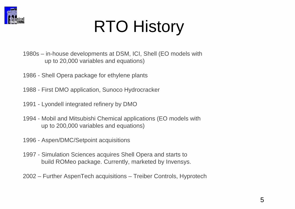
RTO History1980s – in-house developments at DSM, ICI, Shell (EO models with

up to 20,000 variables and equations)

1986 - Shell Opera package for ethylene plants

1988 - First DMO application, Sunoco Hydrocracker

1991 - Lyondell integrated refinery by DMO

1994 - Mobil and Mitsubishi Chemical applications (EO models with up to 200,000 variables and equations)

1996 - Aspen/DMC/Setpoint acquisitions

1997 - Simulation Sciences acquires Shell Opera and starts to build ROMeo package. Currently, marketed by Invensys.

2002 – Further AspenTech acquisitions – Treiber Controls, Hyprotech

5

RTO State of the Art

Aspentech installations (as of 2003)

– Chemicals 10– Ethylene 18– Refining 24– Total 52

Aspentech has about 80% of RTO applications.Others are catching up with newer technology!

ABB , Adersa, DOT Products , Emerson Process Management/MDC,FLS Automation , GE Controls. Gensym, GSE Systems , Honeywell , Invensys PS (Foxboro/SimSci/Esscor) , LIC Energy/ESI , Pavilion Technologies, Shell Global Solutions, SST, STN ATLAS Elektronik, Stoner Associates, Thomson/Thales, Trident Computer Resources, Yokogawa Electric

See http://www.arcweb.com/research/ent/rpo.asp for industry assessment

6

Some Recent RTO Studies

• Agrium - optimization of integrated NH3 plant, 1% improvement in production

• Agip Petroli - FCC CLRTO, $1.4M/yr profit increase• Ecopetrol - FCC RTO, RTOPT with A+ models

• Dow/MDC/Emerson - RTO of system of 4 cogeneration plants, optimization run every 30 min to 2 hours

• PDVSA/SimSci - ROMeo Refinery CLRTO, $7-12K/day gains

• Borealis – Ethylene Plant Optimization (< 9 month payback)• DSM - steam and power utility system optimization, $2.5M

in first year7

RTO - Offline Case Studies

performed at least weekly

0.0

20.0

40.0

60.0

80.0

100.0

%

Explain onlineresults

What if Planning Expansionproject

Other

8

RTO - Basic Concepts

Data Reconciliation & Parameter Identification

•Estimation problem formulations•Steady state model•Maximum likelihood objective functions considered to get parameters (p)

Minp Φ(x, y, p, w)s.t. c(x, u, p, w) = 0

x ∈ X, p ∈ P

Plant

DR-PEc(x, u, p) = 0

RTOc(x, u, p) = 0

APC

y

p

u

w

On line optimization•Steady state model for states (x)•Supply setpoints (u) to APC (control system)•Model mismatch, measured and unmeasured disturbances (w)

Minu F(x, u, w)s.t. c(x, u, p, w) = 0x ∈ X, u ∈ U

9

RTO Characteristics

Plant

DR-PEc(x, u, p) = 0

RTOc(x, u, p) = 0

APC

y

p

u

w

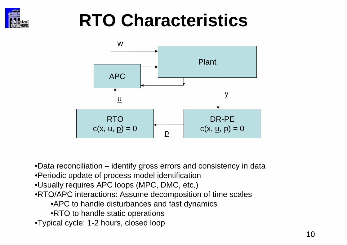
•Data reconciliation – identify gross errors and consistency in data•Periodic update of process model identification •Usually requires APC loops (MPC, DMC, etc.)•RTO/APC interactions: Assume decomposition of time scales

•APC to handle disturbances and fast dynamics•RTO to handle static operations

•Typical cycle: 1-2 hours, closed loop

10

RTO Consistency(Marlin and coworkers)

• How simple is simple?• Plant and RTO model

must be feasible for measurements (y), parameters (p) and setpoints (u)

• Plant and RTO modelmust recognize (close to) same optimum (u*) => satisfy same KKT conditions

• Can RTO model be tuned parametrically to do this?

11

RTO Stability(Marlin and coworkers)

• Stability of APC loop is different from RTO loop

• Is the RTO loop stable to disturbances and input changes?

• How do DR-PE and RTO interact? Can they cycle?

• Interactions with APC and plant?• Stability theory based on small

gain in loop < 1.• Can always be guaranteed by

updating process sufficiently slowly.

Plant

DR-PEc(x, u, p) = 0

RTOc(x, u, p) = 0

APC

y

p

u

w

12

RTO Robustness (Marlin and coworkers)

• What is sensitivity of the optimum to disturbances and model mismatch? => NLP sensitivity

• Are we optimizing on the noise?

• Has the process really changed?

• Statistical test on objective function => change is within a confidence region satisfying a χ2

distribution

• Implement new RTO solution only when the change is significant

• Eliminate ping-ponging13

Model Predictive Control (MPC)

Process

MPC Controller

d : disturbancesz: statesy: outputs

u : manipulatedvariables

ysp : set points

)()(

)()()1(

kCzky

kBukAzkz

=+=+

MPC Estimation and Control

Constraint Other

sConstraint Bound

1-u(u(sp

u

)()()1(..

||))||||)(||min

luBlzAlzts

llylypk

kl

pk

klQQ uy

+=+

−+−∑ ∑+

=

+

=

MPC (QP) Subproblem

Why MPC?

ν Decouple inputs and outputs

ν Handle input and output constraints

ν Reject disturbances and reduce variability

Model Updater

)()(

)()()1(

kCzky

kBukAzkz

=+=+

14

MPC Stability - 1

Nominal stability – perfect model

•Based on Lyapunov argument•Infinite time horizon•Finite time horizon - need endpoint constraints •Dual mode controllers, separate input and output horizons, etc

)1()(,)(

)||))||||)((||

)(

||))||||)(||

||))||||)(||

1

111

1

−→→⇒

−+−=

−≥

−+−=−

−+−=

∑

∑

∑ ∑

∞

=

∞

=−

−

∞

=

∞

=

kukuyky

kkyky

JJJ

kkykyJJ

llylyJ

sp

kQQ

kkk

QQkk

kl klQQk

uy

uy

uy

1-u(u(

1-u(u(

1-u(u(

sp

sp

sp

15

MPC Stability - 2

Analogous property for estimation problem•convergence to state independent of initial condition •use forgetting factors, long horizons

Stable estimator and regulator •separation principle if linear •exponential convergence of estimator if nonlinear•else no guarantees

Robust Stability (unknown w(t), p, model structure? )•Largely an open question•NLP problem formulations (Santos and B., Badgwell,…)•Mismatch as fraction of residual terms 16

Questions Beyond RTO

• Are there limits to on-line solution of NLPs?• - Time-critical • - Large models • + Well-initialized• + Move limits

• APC for dynamics and disturbances, RTO for steady state – what if this is not possible or desirable?

• Should further integration be done for APC and RTO? Fast dynamic optimization?

• Real-world experience?

• What about discrete decisions for time-critical optimization problems?

• Are there inherently dynamic processes where ERP is needed and RTO does not apply?

17

Nonlinear Optimization Engines• Evolution of NLP Solvers:• Î process optimization for design, control

and operations•

’80s: Flowsheet optimization over 100 variables and constraints

‘90s: Static Real-time optimization (RTO)over 100 000 variables and constraints

’00s: Simultaneous dynamic optimizationover 1 000 000 variables and constraints

SQP rSQP IPOPT

rSQP++IPOPT 3.1

Object Oriented Codes to tailor structure, architecture to problems

18

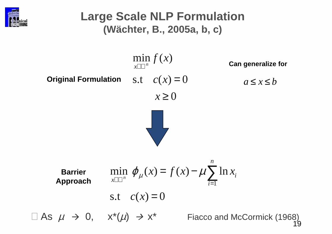
Large Scale NLP Formulation (Wächter, B., 2005a, b, c)

0

0)(s.t

)(min

≥=

ℜ∈

x

xc

xfnx

Original Formulation

0)(s.t

ln)()( min1

=

−= ∑=ℜ∈

xc

xxfxn

ii

x nµϕµBarrier

Approach

Can generalize for

bxa ≤≤

⇒ As µ Æ 0, x*(µ) Æ x* Fiacco and McCormick (1968)19

Solution of the Barrier Problem

⇒ Newton Directions (KKT System)

0 )(

0

0 )()(

==−=−+∇

xc

eXVe

vxAxf

µλ

⇒ Solve

−

−+∇−=

−

− eSv

c

vAf

d

d

d

XV

A

IAQ xT

1

0

00

µ

λ

ν

λ

⇒ Reducing the Systemxv VdXveXd 11 −− −−=µ

∇−=

Σ++ c

d

A

AQ xT

µϕλ

0

VX 1−=Σ

20

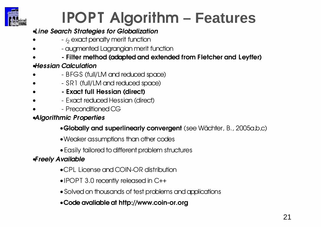
IPOPT Algorithm – Features•L ine Search Strategies for Globalization

• - l2 exact penalty merit function

• - augmented Lagrangian merit function

• - Filter method (adapted and extended from Fletcher and Leyffer)

•Hessian Calculation

• - BFGS (full/LM and reduced space)

• - SR1 (full/LM and reduced space)

• - Exact full Hessian (direct)

• - Exact reduced Hessian (direct)

• - Preconditioned CG

•Algorithmic Properties

•Globally and superlinearly convergent (see Wächter, B., 2005a,b,c)

•Weaker assumptions than other codes

•Easily tailored to different problem structures

•Freely Available

•CPL License and COIN-OR distribution

•IPOPT 3.0 recently released in C++

•Solved on thousands of test problems and applications

•Code avaliable at http://www.coin-or.org

21

Comparison of NLP Solvers: Data Reconciliation

0.01

0.1

1

10

100

0 200 400 600

Degrees of Freedom

CP

U T

ime

(s,

norm

.) LANCELOT

MINOS

SNOPT

KNITRO

LOQO

IPOPT

0

200

400

600

800

1000

0 200 400 600Degrees of Freedom

Itera

tions

LANCELOT

MINOS

SNOPT

KNITRO

LOQO

IPOPT

There is room for growth beyond current technology (e.g, SNOPT)!

22

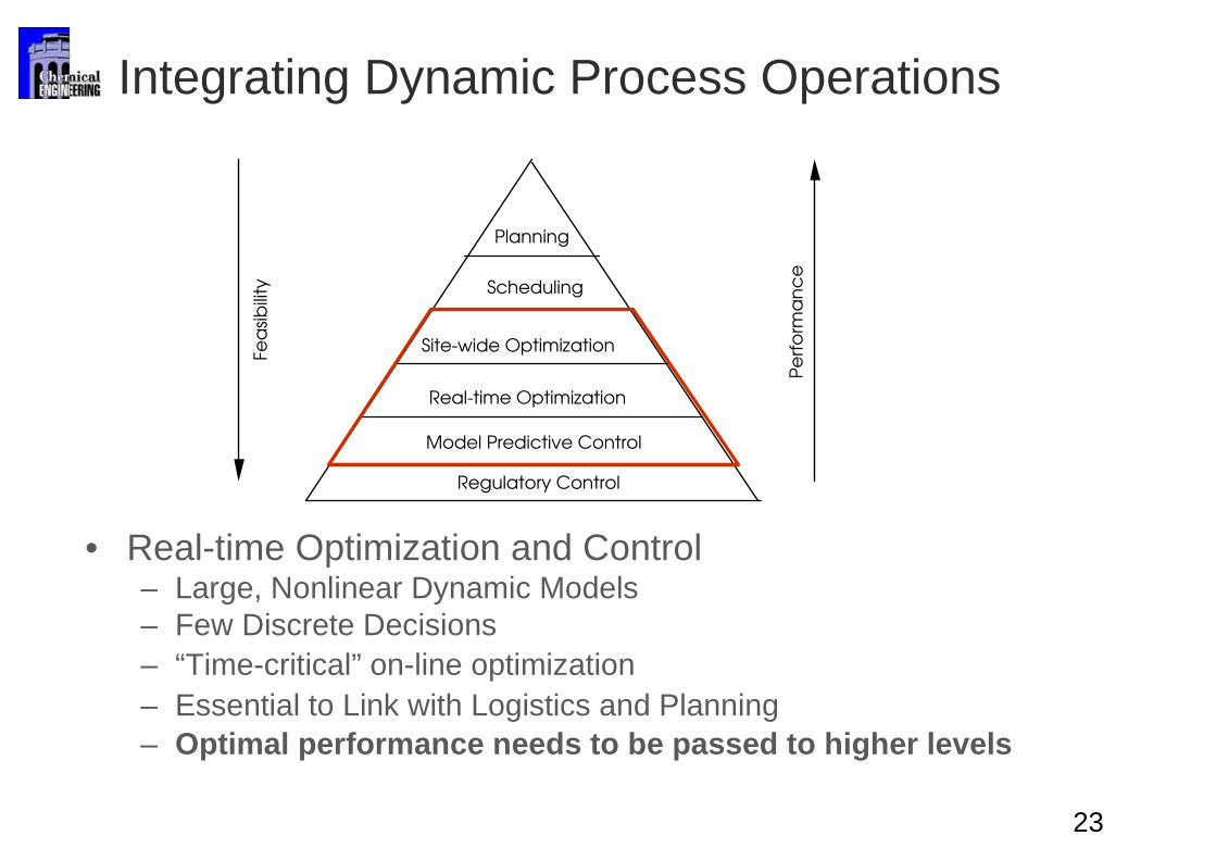
• Real-time Optimization and Control– Large, Nonlinear Dynamic Models– Few Discrete Decisions– “Time-critical” on-line optimization– Essential to Link with Logistics and Planning– Optimal performance needs to be passed to higher levels

Planning

Scheduling

Site-wide Optimization

Real-time Optimization

Model Predictive Control

Regulatory Control

Fe

asi

bili

ty

Pe

rfo

rma

nc

e

Integrating Dynamic Process Operations

23

24

tf, final timeu, control variablesp, time independent parameters

t, timez, differential variablesy, algebraic variables

How is Dynamic Optimization Done?

( )ftp,u(t),y(t),z(t), ψmin

( )pttutytzFdt

tdz,),(),(),(

)( =

( ) 0,),(),(),( =pttutytzG

ul

ul

ul

ul

o

ppp

utuu

ytyy

ztzz

zz

dd

dd

dd

dd

)(

)(

)(

)0(

s.t.

25

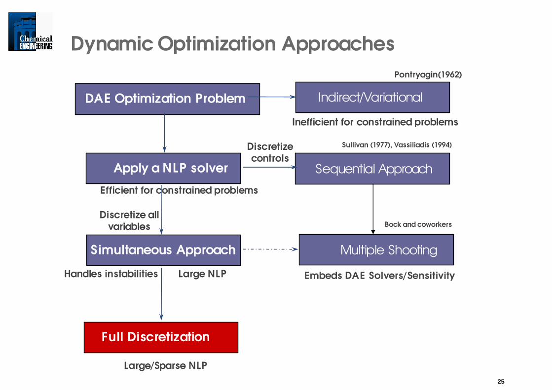
Dynamic Optimization Approaches

DAE Optimization Problem

Multiple Shooting

Embeds DAE Solvers/SensitivityHandles instabilities

Sequential Approach

Sullivan (1977), Vassiliadis (1994)Discretize controls

Full Discretization

Large/Sparse NLP

Apply a NLP solver

Efficient for constrained problems

Simultaneous Approach

Large NLP

Discretize all variables

Indirect/Variational

Pontryagin(1962)

Inefficient for constrained problems

Bock and coworkers

26

Dynamic Optimization StrategiesSummary (Grötschel et al., 2001)

27

to tf

u u u u

Collocation points

• ••• •

•• •

•••

•

True solutionPolynomials

u uu u

•

Finite element, n

tn

Mesh points

h

u u u u

∑=

−− −+=K

1q

q

n

q11n dt

dz(t)g)(zz(t) ntt

u uu

uelement n

q = 1q = 1

q = 2 q = 2 uuuu

∑=

=K

1q

qn

q (t)ygy(t) ∑=

=K

1q

qn

q(t)ugu(t)

Differential variablesDifferential variables

ContinuousContinuous

Algebraic and Control variables

Discontinuous

u

u

u u

(Radau) Collocation on Finite Elements(Radau) Collocation on Finite Elements

28

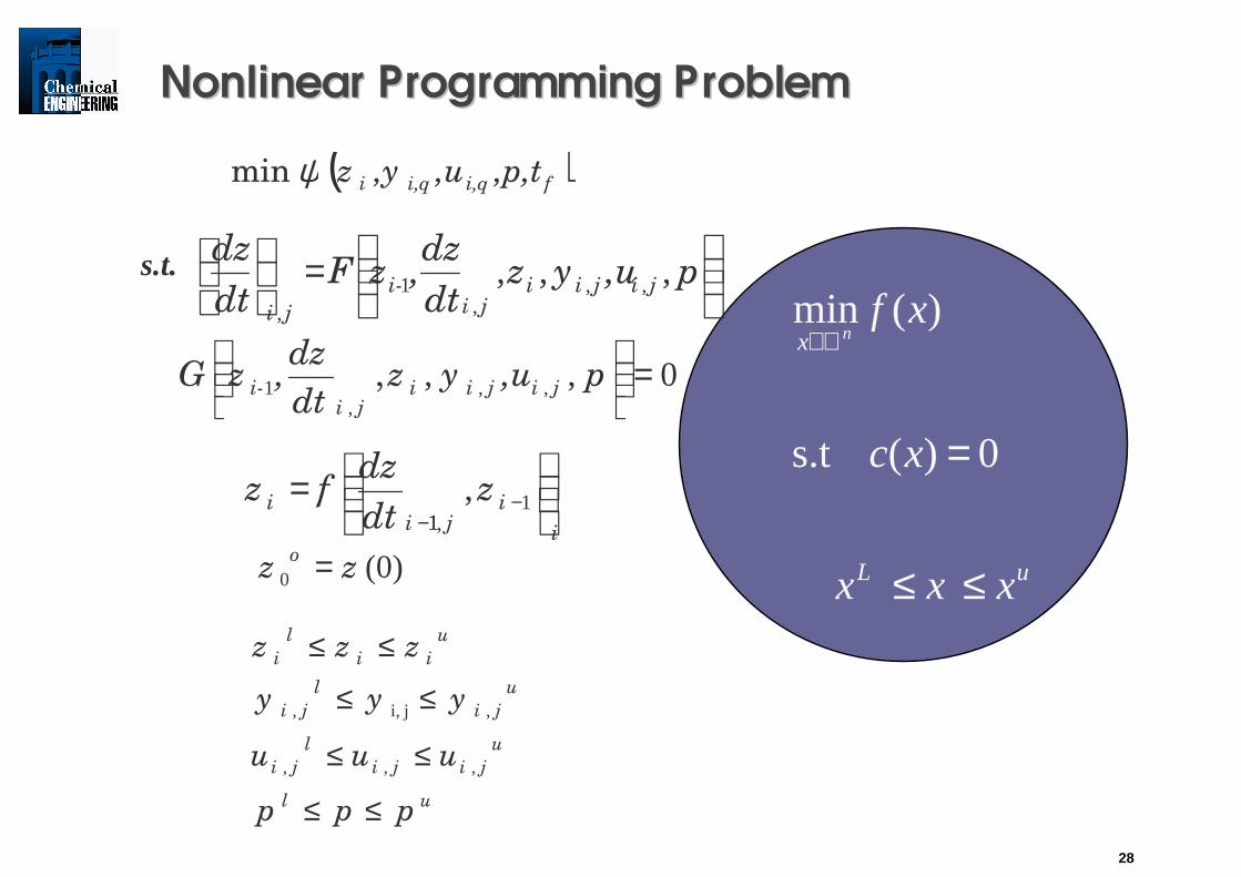
Nonlinear Programming ProblemNonlinear Programming Problem

uL

x

xxx

xc

xfn

≤≤

=

ℜ∈

0)(s.t

)(min

( )fi,qi,qi ,p,t,u,yzψ min

,,, ,,,

1,

=

p,uyzdt

dz,zF

dt

dzjijii

jii-

ji

0,, ,,,

1 =

p,uyzdt

dz,zG jijii

jii- ,

ul

u

jiji

l

ji

u

ji

l

ji

u

ii

l

i

ppp

uuu

yyy

zzz

≤≤

≤≤

≤≤

≤≤

,,,

,ji,,

s.t.

i

iji

i zdt

dzfz

= −

−1

,

,1

(0)0 zzo =

Nonlinear Model Predictive Control (NMPC)

Process

NMPC Controller

d : disturbancesz : differential statesy : algebraic states

u : manipulatedvariables

ysp : set points

( )( )dpuyzG

dpuyzFz

,,,,0

,,,,

==′

NMPC Estimation and Control

ConstraintOther

Constraint Bound

)()),(),(),((0

)),(),(),(()(..

||))||||)(||min

init

1sp

ztztttytzG

tttytzFtzts

yty uy Q

kk

Q

==

=′

−+−∑ ∑ −

u

u

u(tu(tu

NMPC Subproblem

Why NMPC?

ν All benefits of MPC

ν Severe nonlinear dynamics (e.g, sign changes in gains)

ν Operate process over wide range (e.g., startup and shutdown)

ν Deal with more flexible operation (grade changes)

Model Updater( )( )dpuyzG

dpuyzFz

,,,,0

,,,,

==′

29

NMPC for polyolefin processes

Importance of fast grade and flexible grade transitions•Less waste, more production•Performed ~daily

Strong influence on planning and scheduling activitiesOvercome constraints on possible grade changes

AspenTech•applied neural network (BDN) models for NMPC•Significant improvement claimed over conventional control•Generic approach over wide range of polymer processes

Exxon Chemicals•Use fundamental process models•Economics included in NMPC objective function•Benefits of NMPC see in large number of process operations

Planning

Scheduling

Site-wide Optimization

Real-time Optimization

Model Predictive ControlRegulatory Control

30

Planning

Scheduling

Site-wide Optimization

Real-time Optimization

Model Predictive ControlRegulatory Control

NMPC for polyolefin processes(Experience at ExxonMobil Chemicals)

Sampling times: 3 – 6 min.Prediction horizon: 1 hour

31

Reactor Models with LDPE Grade Transition

Cervantes et al. (2000)- 532 DAEs - 83,845 variables- reduced from 5 to 2.7 h

Can more detailed process models (e.g., mile-long tubular reactor) be incorporated into dynamic optimization?)

1.4E-02

1.5E-02

1.6E-02

1.7E-02

1.8E-02

1.9E-02

2.0E-02

2.1E-02

-0.5 0 0.5 1 1.5 2 2.5 3 3.5

Time (hr)

But

ane

com

posi

tion

0

2

4

6

8

10

12

But

ane

Flo

w

w (w t/w t) Flow (kg/h)Zavala et al. (2006)- More detailed reactor model - Accurate parameter estimation with observable parmeters- Plan more detailed dynamic optimizations- AMPL/IPOPT models

Time to reach newsteady state

LDPE out ofspecifications (Ton)

LDPE out ofspecifications ($)

Base case Optimized

1.4 hr 15.4 Ton $7,700

32

33

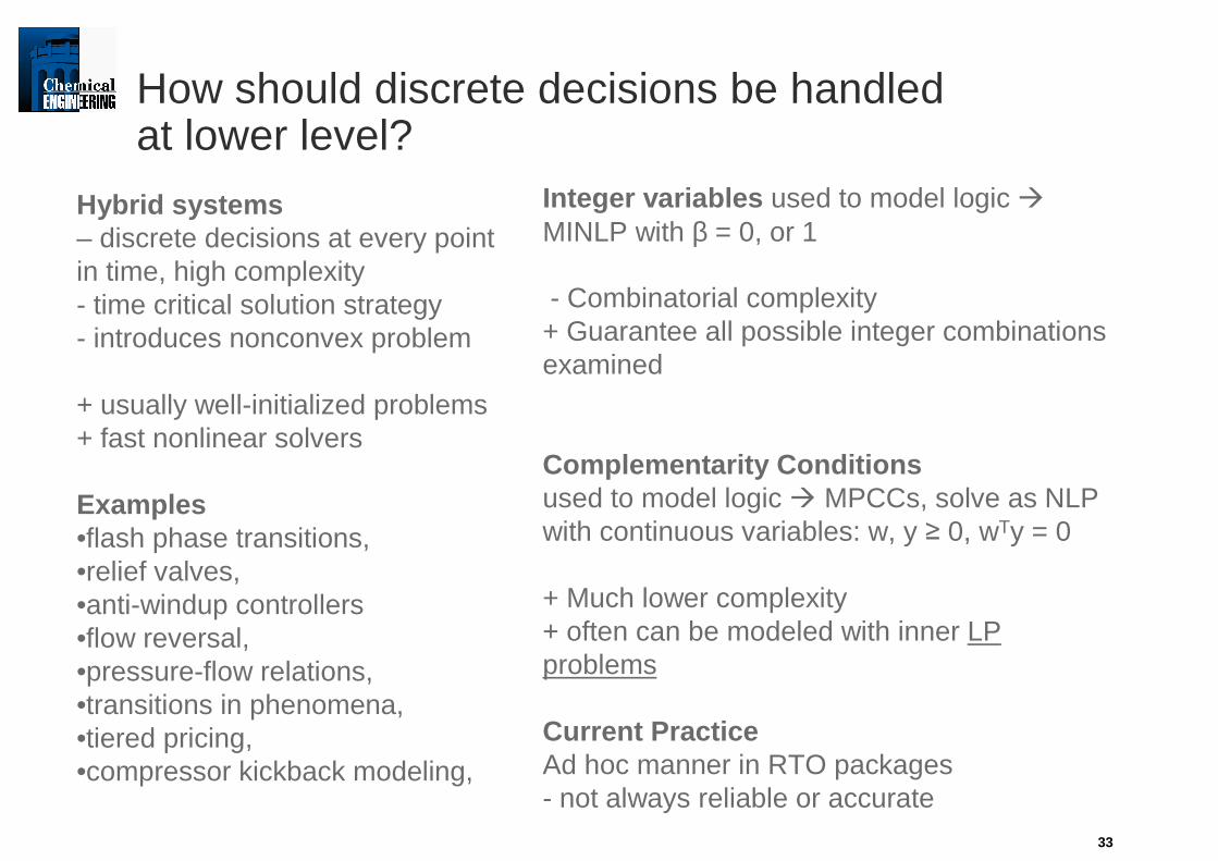
How should discrete decisions be handled at lower level?

Hybrid systems– discrete decisions at every point in time, high complexity- time critical solution strategy - introduces nonconvex problem

+ usually well-initialized problems+ fast nonlinear solvers

Examples•flash phase transitions, •relief valves, •anti-windup controllers•flow reversal, •pressure-flow relations, •transitions in phenomena,•tiered pricing, •compressor kickback modeling,

Integer variables used to model logic ÆMINLP with β = 0, or 1

- Combinatorial complexity+ Guarantee all possible integer combinations examined

Complementarity Conditionsused to model logic Æ MPCCs, solve as NLP with continuous variables: w, y � 0, wTy = 0

+ Much lower complexity+ often can be modeled with inner LP problems

Current PracticeAd hoc manner in RTO packages- not always reliable or accurate

34

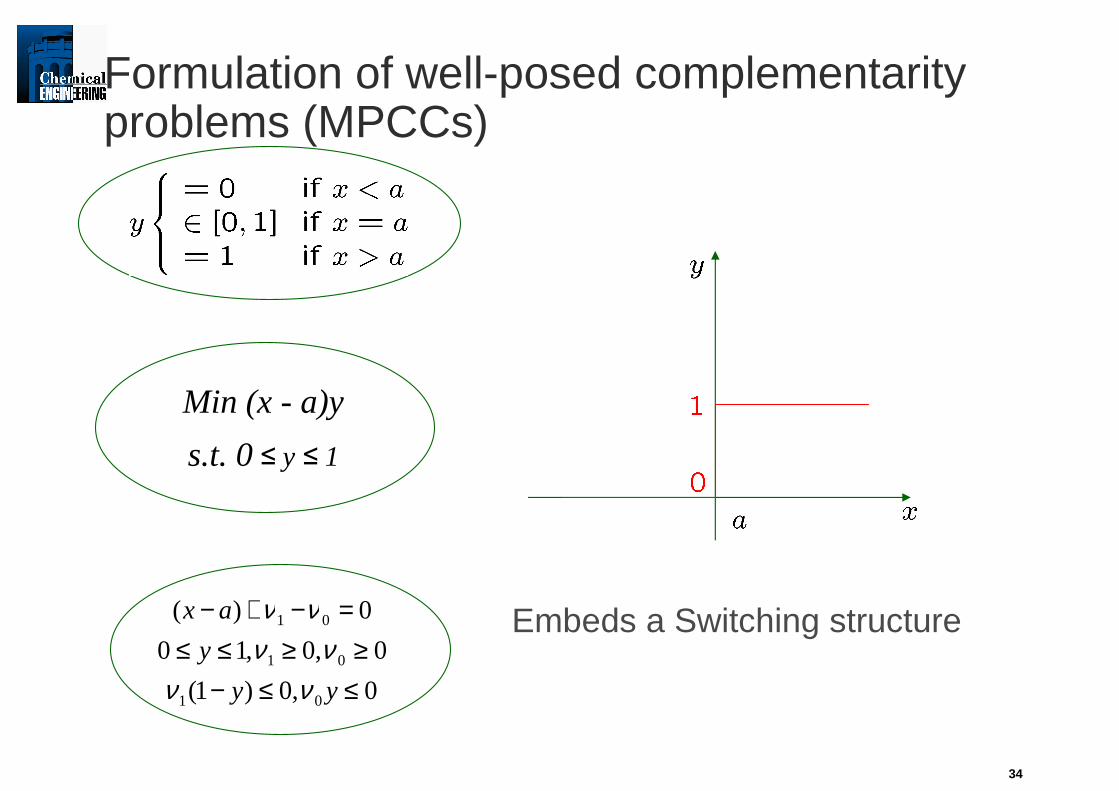
Formulation of well-posed complementarityproblems (MPCCs)

Embeds a Switching structure

Min (x - a)y

s.t. 0 � y � 1

0,0)1(

0,0,10

0)(

01

01

01

≤≤−≥≥≤≤

=−+−

yy

y

ax

νννν

νν

35

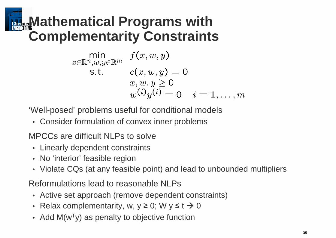
Mathematical Programs with Complementarity Constraints

‘Well-posed’ problems useful for conditional models• Consider formulation of convex inner problems

MPCCs are difficult NLPs to solve• Linearly dependent constraints• No ‘interior’ feasible region• Violate CQs (at any feasible point) and lead to unbounded multipliers

Reformulations lead to reasonable NLPs• Active set approach (remove dependent constraints)• Relax complementarity, w, y � 0; W y � t Æ 0• Add M(wTy) as penalty to objective function

36

MPCCs for Process Optimization using IPOPT(see Biegler Homepage)

Column and Tray Optimization (Raghunathan, B.)

• Binary and 5-component feed

• Ideal thermodynamics

Start-up of distillation columns (Raghunathan, Diaz, B.)

• Batch distillation

• Cryogenic column

Metabolic Networks in Cellular Biology (Raghunathan, Perez, et al.)

• Parameter estimation for batch fermentation

• Optimal control in batch fermentation

Parameter Estimation in Reservoir Flooding Applications (Kameswaran et al.)

• Up to 4300 complementarities, 84000 variables

37

Optimal Cryogenic Distillation Startup Case Study

Pout

• Multi-stage optimization in 3 periods• 8 trays, 10 natural gas components• Dynamic MESH model, vapor holdup• 18000 variables, 575 complementarities

(discrete decisions)

• Complementarity models

F8

L1

V8

F7

Qr

Phase equilibriumLiquid overflow

38

1st Startup Period Establish VLE on All Trays

Ml6 (T) � 10-4Final time constraint

F7 = F8 = 0Feed

QrControls

min TObjective

• Initial charge to bottoms• “inert” component modeled• Require liquid on all but feed trays

0 0.2 0.4 0.60

0.01

0.02

0.03

Time (mins)

Liqu

id H

oldu

p on

tray

s (k

mol

)

Tray2Tray3Tray4Tray5Tray6Tray7Tray8

0 0.2 0.4 0.60.1

0.2

0.3

0.4

0.5

0.6

0.7

0.8

0.9

1

Time (mins)

β i

Tray1Tray2Tray3Tray4Tray5Tray6Tray7Tray8

39

2nd Startup PeriodSufficient Holdup on All Trays

L2(T) > 1Final time constraint

F7 = 30, F8 = 100Feed

Pout, QrControls

min T + 0.1�0TQr dtObjective• F8 mostly vapor• Require liquid flow from all trays

0 0.2 0.4 0.6 0.8 1 1.2 1.40

2

4

6

8

10

12

Time (mins)

Liqu

id H

oldu

p on

tray

s (k

mol

)

Tray1Tray2Tray3Tray4Tray5Tray6Tray7Tray8F8

L1

V8

F7

Qr

Pout

40

Can EWO be applied to inherently dynamic processes?

Batch processes – integration of scheduling with dynamic optimization•Bhatia, B. (1997)•Harjunkoski et al. (2004)•Flores, Grossmann (2006)

Simulated Moving Beds (SMB)• Developed at UOP in 1960s• Operate dynamically with periodic boundary conditions• Petrochemical (Xylene isomers)• Sugars (Fructose/glucose separation)

High fructose corn syrup• Pharmaceuticals (Enantiomeric separation)

Separate ‘good’ from ‘bad’ compounds based on chirality

41

Chromatography: Exploit different affinities to adsorbent

Column, packed with adsorbent

1. Initial stateColumn is filled with desorbent

Desorbent DesorbentFeed(fructose + glucose)

2. FeedFeed is supplied at the end

Desorbent

3. ElutionPush the feed to the other endTwo components separates as moving toward the end

(Difference in affinity)

Glucose product

4, Recovery of 1st product

Fructose product

5. Recovery of 2nd product

Challenge: make batch process Challenge: make batch process ÆÆ continuouscontinuous

42

Chromatography Column Model

Mass balance in liquid phase

Mass balance in solid phase

Isotherm (Linear)

Overall Mass Transfer Coeff.

Concentration in the solid phase

Concentration in the liquid phase

Void fraction

Liquid velocity

Subscripts n : Column number

i : Component

43

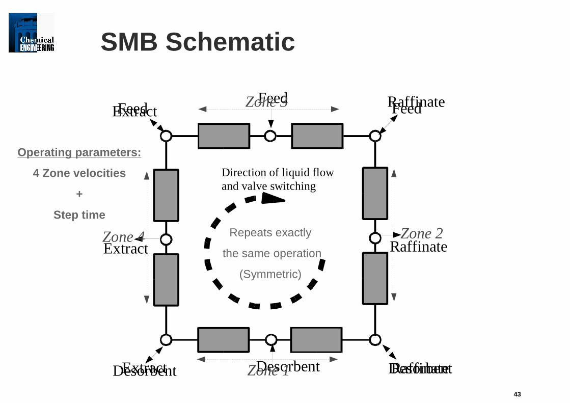
SMB Schematic

Direction of liquid flowand valve switching

Feed

Raffinate

Desorbent

ExtractRepeats exactly

the same operation

(Symmetric)

Feed Raffinate

DesorbentExtract

Operating parameters:

4 Zone velocities

+

Step time

Zone 4 Zone 2

Zone 3

Zone 1

Feed

RaffinateDesorbent

Extract

44

Dynamic Optimization of SMB

CPU Time*

Single discretization 111.8 min

1.53 minFull discretization

# of iteration

49

47

0 1 2 3 4 5 6 7 8−0.1

0

0.1

0.2

0.3

0.4

0.5

0.6

0.7

0.8

x [m]

Nor

mal

ized

Con

cenr

atio

n, C

i(x,t st

ep)/

CF

,i

Comp.1 Single discretizationComp.2 Single discretizationComp.1 Full discretizationComp.2 Full discretization

Both single, full discretization methods find same optimal solution

# of variables

33999

644Implemented on gPROMS, solved using SRQPDImplemented on gPROMS, solved using SRQPD

Implemented on AMPL, solved using IPOPTImplemented on AMPL, solved using IPOPT

*On Pentium IV 2.8GHz

(89% spent by integrator)

(Linear isotherm)

45

Glucose/Fructose SeparationVariable flow rates (PowerFeed)

Dynamic problem definition, same as with constant feed

Optimal UF: 1.074 [m/h]

(productivity: double constant feed case)

CPU Time: 5.45 min

Number of Iterations: 84

Simultaneous Method

(Implemented on AMPL/IPOPT)Optimal Control Profile

Optimization Implications:

•Higher performance and higher purity•New SMB designs developed•Extensions to develop on-line dynamic optimization

Summary

• RTO is essential for refineries, ethylene and, more recently, chemical plants - not competitive otherwise.

• Current and developing large-scale NLP tools are well-suited to these tasks. Can also be done on-line and extended to deal with dynamics.

• Dynamic optimization is essential for a number of processes– Polymer processes (especially grade transitions)– Batch processes– Periodic processes

• Lower level discrete decisions can be handled through (well-formulated) MPCCs.

46

ReferencesF. Allgöwer and A. Zheng (eds.), Nonlinear Model Predictive Control, Birkhaeuser, Basel (2000)

R. D. Bartusiak, “NLMPC: A platform for optimal control of feed- or product-flexible manufacturing,” in Nonlinear Model Predictive Control 05, Allgower, Findeisen, Biegler (eds.), Springer, to appear

Biegler Homepage: http://dynopt.cheme.cmu.edu/papers.htm

Forbes, J. F. and Marlin, T. E.. Model Accuracy for Economic Optimizing Controllers: The Bias Update Case. Ind.Eng.Chem.Res. 33, 1919-1929. 1994

Forbes, J. F. and Marlin, T. E.. “Design Cost: A Systematic Approach to Technology Selection for Model-Based Real-Time Optimization Systems,” Computers Chem.Engng. 20[6/7], 717-734. 1996

Grossmann Homepage: http://egon.cheme.cmu.edu/papers.html

M. Grötschel, S. Krumke, J. Rambau (eds.), Online Optimization of Large Systems, Springer, Berlin (2001)

K. Naidoo, J. Guiver, P. Turner, M. Keenan, M. Harmse “Experiences with Nonlinear MPC in Polymer Manufacturing,” in Nonlinear Model Predictive Control 05, Allgower, Findeisen, Biegler(eds.), Springer, to appear

Yip, W. S. and Marlin, T. E. “Multiple Data Sets for Model Updating in Real-Time Operations Optimization,” Computers Chem.Engng. 26[10], 1345-1362. 2002.

47