Dynamic Programming and Optimal Control Volume 1 SECOND EDITION Dimitri P. Bertsekas Massachusetts Institute of Technology Selected Theoretical Problem Solutions Athena Scientific, Belmont, MA, 2000 WWW site for book information and orders http://www.athenasc.com/ 1
Transcript
Dynamic Programming and Optimal Control
Volume 1
SECOND EDITION
Dimitri P. Bertsekas
Massachusetts Institute of Technology
Selected Theoretical Problem Solutions
Athena Scientific, Belmont, MA, 2000
WWW site for book information and orders
http://www.athenasc.com/
1
NOTE
This solution set is meant to be a significant extension of the scope and coverage of the book. Solutions to
all of the book’s exercises marked with the symbol www have been included. The solutions are continuously
updated and improved, and additional material, including new problems and their solutions are being added.
The solutions may be reproduced and distributed for personal or educational uses. Please send comments,
and suggestions for additions and improvements to the author at
Note that E{Ak} and E{wk} do not depend on xk or uk. If the optimal value is finite then min{gk(uk) +b′k+1fk(uk)} is a real number and Jk(xk) is affine. Furthermore, the optimal control at each stage solves thisminimization which is independent of xk. Thus, the optimal policy consists of constant functions µ∗k.
4
1.16 www
(a) Given a sequence of matrix multiplications
M1M2 · · ·MkMk+1 · · ·MN
we represent it by a sequence of numbers {n1, . . . , nN+1}, where nk × nk+1 is the dimension of Mk. Let theinitial state be x0 = {n1, . . . , nN+1}. Then choosing the first multiplication to be carried out corresponds tochoosing an element from the set x0−{n1, nN+1}. For instance, choosing n2 corresponds to multiplying M1
and M2, which results in a matrix of dimension n1×n3, and the initial state must be updated to discard n2,the control applied at that stage. Hence at each stage the state represents the dimensions of the matricesresulting from the multiplications done so far. The allowable controls at stage k are uk ∈ xk − {n1, nN+1}.The system equation evolves according to
xk+1 = xk − uk.
Note that the control will be applied N − 1 times, therefore the horizon of this problem is N − 1. Theterminal state is xN−1 = {n1, nN+1} and the terminal cost is 0. The cost at stage k is given by the numberof multiplications,
gk(xk, uk) = nanuknb,
where nuk= uk and
a = max{i ∈ {1, . . . , N + 1} | i < uk, i ∈ xk
},
b = min{i ∈ {1, . . . , N + 1} | i > uk, i ∈ xk
}.
The DP algorithm for this problem is given by
JN−1(xN−1) = 0,
Jk(xk) = minuk∈xk−{n1,nN+1}
{nanuk
nb + Jk+1(xk − uk)}
, k = 0, . . . , N − 2.
Now consider the given problem, where N = 3 and
M1 is 2× 10
M2 is 10× 5
M3 is 5× 1
The optimal order is M1(M2M3), requiring 70 multiplications.
(b) In this part we can choose a much simpler state space. Let the state at stage k be given by {a, b}, wherea, b ∈ {1, . . . ,N} and give the indices of the first and the last matrix in the current partial product. Thereare two possible controls at each stage, which we denote by L and R. Note that L can be applied only whena 6= 1 and R can be applied only when b 6= N . The system equation evolves according to
xk+1 =
{{a− 1, b}, if uk = L{a, b + 1}, if uk = R
k = 1, . . . ,N − 1.
The terminal state is xN = {1, N} with cost 0. The cost at stage k is given by
gk(xk, uk) =
{na−1nanb+1, if uk = Lnanb+1nb+2, if uk = R
k = 1, . . . , N − 1.
To handle the initial stage, we can take x0 to be the empty set and u0 ∈ {1, . . . , N}. The next state will begiven by x1 = {u0, u0} and the cost incurred at the initial stage will be 0 for all possible controls.
5
1.19 www
Let t1 < t2 < . . . < tN−1 denote the times where g1(t) = g2(t). Clearly, it is never optimal to switchfunctions at any other times. We can therefore divide the problem into N − 1 stages, where we want todetermine for each stage k whether or not to switch activities at time tk.
Define
xk =
{0 if on activity g1 just before time tk
1 if on activity g2 just before time tk
uk =
{0 to continue current activity1 to switch between activities
Then the state at time tk+1 is simply xk+1 = (xk + uk) mod 2, and the profit for stage k is
gk(xk, uk) =
∫ tk+1
tk
g1+xk+1(t)dt− ukc
The DP algorithm is then
JN (xN ) = 0
Jk(xk) = minuk
{gk(xk, uk) + Jk+1[(xk + uk) mod 2]} .
1.24 www
(a) Consider the problem with the state equal to the number of free rooms. At state x ≥ 1 with y customersremaining, if the inkeeper quotes a rate ri, the transition probability is pi to state x− 1 (with a reward ofri) and 1− pi to state x (with a reward of 0). The DP algorithm for this problem starts with the terminalconditions
J(x, 0) = J(0, y) = 0, ∀ x ≥ 0, y ≥ 0,
and is given by
J(x, y) = maxi=1,...,m
[pi(ri + J(x− 1, y − 1)) + (1− pi)J(x, y − 1)
], ∀ x ≥ 0.
From the above equation and the terminal conditions, we can compute sequentially J(1, 1), J(1, 2), . . . , J(1, y)up to any desired integer y. Then, we can calculate J(2, 1), J(2, 2), . . . , J(2, y), etc.
We first prove by induction on y that for all y, we have
J(x, y) ≥ J(x− 1, y), ∀ x ≥ 1.
Indeed this is true for y = 0. Assuming this is true for a given y, we will prove that
J(x, y + 1) ≥ J(x− 1, y + 1), ∀ x ≥ 1.
This relation holds for x = 1 since ri > 0. For x ≥ 2, by using the DP recursion, this relation is written as
maxi=1,...,m
[pi(ri + J(x− 1, y)) + (1− pi)J(x, y)
]≥ max
i=1,...,m
[pi(ri + J(x− 2, y)) + (1− pi)J(x− 1, y)
].
6
By the induction hypothesis, each of the terms on the left-hand side is no less than the corresponding termon the right-hand side, so the above relation holds.
The optimal rate is the one that maximizes in the DP algorithm, or equivalently, the one that maximizes
piri + pi(J(x− 1, y − 1)− J(x, y − 1)).
The highest rate rm simultaneously maximizes piri and minimizes pi. Since
J(x− 1, y − 1)− J(x, y − 1) ≤ 0,
as proved above, we see that the highest rate simultaneously maximizes piri and pi(J(x−1, y−1)−J(x, y−1)),and so it maximizes their sum.
(b) The algorithm given is the algorithm of Exercise 1.22 applied to the problem of part (a). Clearly, it isoptimal to accept an offer of ri if ri is larger than the threshold
r(x, y) = J(x, y − 1)− J(x− 1, y − 1).
1.25 www
(a) The total net expected profit from the (buy/sell) investment decissions after transaction costs are de-ducted is
E
{N−1∑
k=0
(ukPk(xk)− c |uk|
)}
,
where
uk =
{1 if a unit of stock is bought at the kth period,−1 if a unit of stock is sold at the kth period,0 otherwise.
With a policy that maximizes this expression, we simultaneously maximize the expected total worth of thestock held at time N minus the investment costs (including sale revenues).
The DP algorithm is given by
Jk(xk) = maxuk=−1,0,1
[ukPk(xk)− c |uk|+ E
{Jk+1(xk+1) | xk
}],
withJN (xN ) = 0,
where Jk+1(xk+1) is the optimal expected profit when the stock price is xk+1 at time k + 1. Since uk doesnot influence xk+1 and E
{Jk+1(xk+1) | xk
}, a decision uk ∈ {−1, 0,1} that maximizes ukPk(xk) − c |uk| at
time k is optimal. Since Pk(xk) is monotonically nonincreasing in xk, it follows that it is optimal to set
uk =
{1 if xk ≤ xk,−1 if xk ≥ xk,0 otherwise,
where xk and xk are as in the problem statement. Note that the optimal expected profit Jk(xk) is given by
Jk(xk) = E
{N−1∑
i=k
maxui=−1,0,1
[uiPi(xi) − c |ui|
]}
.
7
(b) Let nk be the number of units of stock held at time k. If nk is less that N −k (the number of remainingdecisions), then the value nk should influence the decision at time k. We thus take as state the pair (xk, nk),and the corresponding DP algorithm takes the form
Vk(xk, nk) =
maxuk∈{−1,0,1}[ukPk(xk)− c |uk|+ E
{Vk+1(xk+1, nk + uk) | xk
}]if nk ≥ 1,
maxuk∈{0,1}[ukPk(xk) − c |uk|+ E
{Vk+1(xk+1, nk + uk) | xk
}]if nk = 0,
withVN (xN , nN ) = 0.
Note that we haveVk(xk, nk) = Jk(xk), if nk ≥ N − k,
where Jk(xk) is given by the formula derived in part (a). Using the above DP algorithm, we can calculateVN−1(xN−1, nN−1) for all values of nN−1, then calculate VN−2(xN−2, nN−2) for all values of nN−2, etc.
To show the stated property of the optimal policy, we note that Vk(xk, nk) is monotonically nondecreasingwith nk, since as nk decreases, the remaining decisions become more constrained. An optimal policy at timek is to buy if
Pk(xk)− c + E{Vk+1(xk+1, nk + 1) − Vk+1(xk+1, nk) | xk
}≥ 0, (1)
and to sell if−Pk(xk) − c + E
{Vk+1(xk+1, nk − 1)− Vk+1(xk+1, nk) | xk
}≥ 0. (2)
The expected value in Eq. (1) is nonnegative, which implies that if xk ≤ xk, implying that Pk(xk)− c ≥ 0,then the buying decision is optimal. Similarly, the expected value in Eq. (2) is nonpositive, which impliesthat if xk < xk, implying that −Pk(xk) − c < 0, then the selling decision cannot be optimal. It is possiblethat buying at a price greater than xk is optimal depending on the size of the expected value term in Eq.(1).
(c) Let mk be the number of allowed purchase decisions at time k, i.e., m plus the number of sale decisionsup to k, minus the number of purchase decisions up to k. If mk is less than N − k (the number of remainingdecisions), then the value mk should influence the decision at time k. We thus take as state the pair (xk, mk),and the corresponding DP algorithm takes the form
Wk(xk, mk) =
maxuk∈{−1,0,1}[ukPk(xk)− c |uk|+ E
{Wk+1(xk+1, mk − uk) | xk
}]if mk ≥ 1,
maxuk∈{−1,0}[ukPk(xk)− c |uk|+ E
{Wk+1(xk+1,mk − uk) | xk
}]if mk = 0,
withWN (xN , mN ) = 0.
From this point the analysis is similar to the one of part (b).
(d) The DP algorithm takes the form
Hk(xk, mk, nk) = maxuk∈{−1,0,1}
[ukPk(xk) − c |uk|+ E
{Hk+1(xk+1, mk − uk, nk + uk) | xk
}]
if mk ≥ 1 and nk ≥ 1, and similar formulas apply for the cases where mk = 0 and/or nk = 0 [compare withthe DP algorithms of parts (b) and (c)].
(e) Let r be the interest rate, so that x invested dollars at time k will become (1 + r)N−kx dollars at timeN . Once we redefine the expected profit Pk(xk) to be
Pk(x) = E{xN | xk = x} − (1 + r)N−kx,
the preceding analysis applies.
8
1.27 www
We consider part (b), since part (a) is essentially a special case. We will consider the problem of placingN −2 points between the endpoints A and B of the given subarc. We will show that the polygon of maximalarea is obtained when the N − 2 points are equally spaced on the subarc between A and B. Based ongeometric considerations, we impose the restriction that the angle between any two successive points is nomore than π.
As the subarc is traversed in the clockwise direction, we number sequentially the encountered points asx1, x2, . . . , xN , where x1 and xN are the two endpoints A and B of the arc, respectively. For any point xon the subarc, we denote by φ the angle between x and xN (measured clockwise), and we denote by Ak(φ)the maximal area of a polygon with vertices the center of the circle, the points x and xN , and N − k − 1additional points on the subarc that lie between x and xN .
Without loss of generality, we assume that the radius of the circle is 1, so that the area of the trianglethat has as vertices two points on the circle and the center of the circle is (1/2) sinu, where u is the anglecorresponding to the center.
By viewing as state the angle φk between xk and xN , and as control the angle uk between xk and xk+1,we obtain the following DP algorithm
Ak(φk) = max0≤uk≤min{φk,π}
[1
2sinuk + Ak+1(φk − uk)
], k = 1, . . . ,N − 2. (1)
Once xN−1 is chosen, there is no issue of further choice of a point lying between xN−1 and xN , so we have
AN−1(φ) =1
2sinφ, (2)
using the formula for the area of the triangle formed by xN−1, xN , and the center of the circle.
It can be verified by induction that the above algorithm admits the closed form solution
Ak(φk) =1
2(N − k) sin
(φk
N − k
), k = 1, . . . ,N − 1, (3)
and that the optimal choice for uk is given by
u∗k =φk
N − k.
Indeed, the formula (3) holds for k = N − 1, by Eq. (2). Assuming that Eq. (3) holds for k + 1, we havefrom the DP algorithm (1)
Ak(φk) = max0≤uk≤min{φk,π}
Hk(uk, φk), (4)
where
Hk(uk, φk) =1
2sinuk +
1
2(N − k − 1) sin
(φk − uk
N − k − 1
). (5)
It can be verified that for a fixed φk and in the range 0 ≤ uk ≤ min{φk, π}, the function Hk(·, φk) is concave(its second derivative is negative) and its derivative is 0 only at the point u∗k = φk/(N − k) which musttherefore be its unique maximum. Substituting this value of u∗k in Eqs. (4) and (5), we obtain
Ak(φk) =1
2sin
(φk
N − k
)+
1
2(N − k − 1) sin
(φk − φk/(N − k)
N − k − 1
)=
1
2(N − k) sin
(φk
N − k
),
and the induction is complete.
Thus, given an optimally placed point xk on the subarc with corresponding angle φk, the next point xk+1
is obtained by advancing clockwise by φk/(N − k). This process, when started at x1 with φ1 equal to theangle between x1 and xN , yields as the optimal solution an equally spaced placement of the points on thesubarc.
9
Vol. I, Chapter 2
2.4 www
(a) We denote by Pk the OPEN list after having removed k nodes from OPEN, (i.e., after having performedk iterations of the algorithm). We also denote dk
j the value of dj at this time. Let bk = minj∈Pk{dkj }. First,
we show by induction that b0 ≤ b1 ≤ · · · ≤ bk. Indeed, b0 = 0 and b1 = minj{asj} ≥ 0, which implies thatb0 ≤ b1. Next, we assume that b0 ≤ · · · ≤ bk for some k ≥ 1; we shall prove that bk ≤ bk+1. Let jk+1 be thenode removed from OPEN during the (k + 1)th iteration. By assumption dk
jk+1= minj∈Pk{dk
j} = bk, and
we also have
dk+1i = min{dk
i , dkjk+1
+ ajk+1i}.
We have Pk+1 = (Pk − {jk+1}) ∪Nk+1, where Nk+1 is the set of nodes i satisfying dk+1i = dk
jk+1+ ajk+1i
and i /∈ Pk. Therefore,
mini∈Pk+1
{dk+1i } = min
i∈(Pk−{jk+1})∪Nk+1
{dk+1i } = min
[min
i∈Pk−{jk+1}{dk+1
i }, mini∈Nk+1
{dk+1i }
].
Clearly,
mini∈Nk+1
{dk+1i } = min
i∈Nk+1
{dkjk+1
+ ajk+1i} ≥ dkjk+1
.
Moreover,
mini∈Pk−{jk+1}
{dk+1i } = min
i∈Pk−{jk+1}
[min{dk
i , dkjk+1
+ ajk+1i}]
≥ min
[min
i∈Pk−{jk+1}{dk
i }, dkjk+1
]= min
i∈Pk
{dki } = dk
jk+1,
because we remove from OPEN this node with the minimum dki . It follows that bk+1 = mini∈Pk+1{dk+1
i } ≥dk
jk+1= bk.
Now, we may prove that once a node exits OPEN, it never re-enters. Indeed, suppose that some node i
exits OPEN after the k∗th iteration of the algorithm; then, dk∗−1i = bk∗−1. If node i re-enters OPEN after
the `∗th iteration (with `∗ > k∗), then we have d`1−1i > d`∗
i = d`∗−1j∗`
+ aj`∗ i ≥ d`∗−1j`∗
= b`∗−1. On the other
hand, since di is non-increasing, we have bk∗−1 = dk∗−1i ≥ d`∗−1
i . Thus, we obtain bk∗−1 > b`∗−1, whichcontradicts the fact that bk is non-decreasing.
Next, we claim the following: after the kth iteration, dki equals the length of the shortest possible path
from s to node i ∈ Pk under the restriction that all intermediate nodes belong to Ck. The proof will be doneby induction on k. For k = 1, we have C1 = {s} and d1
i = asi, and the claim is obviously true. Next, weassume that the claim is true after iterations 1, . . . , k; we shall show that it is also true after iteration k + 1.The node jk+1 removed from OPEN at the (k + 1)-st iteration satisfies mini∈Pk
{dki } = d∗jk+1
. Notice now
that all neighbors of the nodes in Ck belong either to Ck or to Pk.
It follows that the shortest path from s to jk+1 either goes through Ck or it exits Ck, then it passesthrough a node j∗ ∈ Pk, and eventually reaches jk+1. If the latter case applies, then the length of this pathis at least the length of the shortest path from s to j∗ through Ck; by the induction hypothesis, this equalsdk
j∗ , which is at least dkjk+1
. It follows that, for node jk+1 exiting the OPEN list, dkjk+1
equals the length of
the shortest path from s to jk+1. Similarly, all nodes that have exited previously have their current estimate
10
of di equal to the corresponding shortest distance from s. * Notice now that
dk+1i = min
{dk
i , dkjk+1
+ ajk+1i
}.
For i /∈ Pk and i ∈ Pk+1 it follows that the only neighbor of i in Ck+1 = Ck ∪ {jk+1} is node jk+1; forsuch a node i, dk
i = ∞, which leads to dk+1i = dk
jk+1+ ajk+1i. For i 6= jk+1 and i ∈ Pk, the augmentation
of Ck by including jk+1 offers one more path from s to i through Ck+1, namely that through jk+1. Recallthat the shortest path from s to i through Ck has length dk
i (by the induction hypothesis). Thus, dk+1i =
min{dk1, d
kjk+1
+ ajk+1i
}is the length of the shortest path from s to i through Ck+1.
The fact that each node exits OPEN with its current estimate of di being equal to its shortest distancefrom s has been proved in the course of the previous inductive argument.
(b) Since each node enters the OPEN list at most once, the algorithm will terminate in at most N − 1iterations. Updating the di’s during an iteration and selecting the node to exit OPEN requires O(N )arithmetic operations (i.e., a constant number of operations per node). Thus, the total number of operationsis O(N 2).
2.6 www
Proposition: If there exist a path from the origin to each node in T , the modified version of the labelcorrecting algorithm terminates with UPPER < ∞ and yields a shortest path from the origin to each nodein T . Otherwise the algorithm terminates with UPPER = ∞.
Proof: The proof is analogous to the proof of Proposition 3.1. To show that this algorithm terminates, wecan use the identical argument in the proof of Proposition 3.1.
Now suppose that for some node t ∈ T , there is no path from s to t. Then a node i such that (i, t) is anarc cannot enter the OPEN list because this would establish that there is a path from s to i, and thereforealso a path from s to t. Thus, dt is never changed and UPPER is never reduced from its initial value of ∞.
Suppose now that there is a path from s to each node t ∈ T . Then, since there is a finite number ofdistinct lengths of paths from s to each t ∈ T that do not contain any cycles, and each cycle has nonnegativelength, there is also a shortest path. For some arbitrary t, let (s, j1, j2, . . . , jk, t) be a shortest path andlet d∗t be the corresponding shortest distance. We will show that the value of UPPER upon terminationmust be equal to d∗ = maxt∈T d∗t . Indeed, each subpath (s, j1, . . . , jm),m = 1, . . . , k, of the shortest path(s, j1, . . . , jk, t) must be a shortest path from s to jm. If the value of UPPER is larger than d∗ at termination,the same must be true throughout the algorithm, and therefore UPPER will also be larger than the lengthof all the paths (s, j1, . . . , jm), m = 1, . . . , k, throughout the algorithm, in view of the nonnegative arc lengthassumption. If, for each t ∈ T , the parent node jk enters the OPEN list with djk equal to the shortestdistance from s to jk, UPPER will be set to d∗ in step 2 immediately following the next time the last ofthe nodes jk is examined by the algorithm in step 2. It follows that, for some t ∈ T , the associated parentnode jk will never enter the OPEN list with djk
equal to the shortest distance from s to jk. Similarly, andusing also the nonnegative length assumption, this means that node jk−1 will never enter the OPEN listwith djk−1
equal to the shortest distance from s to jk−1. Proceeding backwards, we conclude that j1 never
enters the OPEN list with dj1equal to the shortest distance from s to j1 [which is equal to the length of
the arc (s, j1)]. This happens, however, at the first iteration of the algorithm, obtaining a contradiction. Itfollws that at termination, UPPER will be equal to d∗.
Finally, it can be seen that, upon termination of the algorithm, the path constructed by tracing the parentnodes backward from d to s has length equal to d∗t for each t ∈ T . Thus the path is a shortest path from sto t.
* Strictly speaking, this is the shortest distance from s to these nodes because paths are directed from s tothe nodes.
11
2.9 www
(a) It was shown in the proof to proposition 3.2 that (P, p) satisfies CS throughout the original algorithm.Note that deleting arcs does not cause CS conditions to no longer hold. Therefore (P, p) satisfies CSthroughout this algorithm. It was also shown in the text that if a pair (P, p) satisfies the CS conditions, thenthe portion of the path P between node s and any node i ∈ P is a shortest path from s to i. Now, considerany node j that becomes the terminal node of P through an extension using (i, j). If there is a shortest pathfrom s to t that does not include node j, then removing the arcs (k, j) where k 6= i yields a graph includingthe same shortest path. If the only shortest path from s to t does include node j, then since P is a shortestpath from s to j, there is a shortest path from s to t that has P as its portion to node j. Thus removingthe arcs (k, j), where k 6= i yields a graph including a shortest path from the original graph. If node j hasno outgoing arcs, then any path from s to t can not include j. Thus removing j yields a graph includingthe same paths from s to t as in the original graph. Therefore, both types of arc deletions leave the shortestdistance from s to t unaffected.
We can view the auction algorithm with graph reduction as follows: an iteration of the original auctionalgorithm is applied, followed by arc deletions that do not affect the CS conditions and which leaves theshortest distance from s to t unchanged; another iteration of the original auction algorithm is applied to thenew graph, follwed by arc deletions; and so on. If an iteration of the original auction algorithm yields a pathP with t as the terminal node, P is a shortest path from s to t in the latest modified graph. Since we haveshown that each new graph has the same shortest distance from s to t as in the original graph, P must alsobe a shortest path from s to t in the original graph.
Now assume that no iteration of the original auction algorithm ever yields a path P with t as the terminalnode; i.e., there is no path from s to t. Assume that the modified algorithm never terminates. Since thereare a finite number of arcs and nodes, there can be only a finite number of arc and node deletions. Considerthe algorithm after the last deletion. Since there are no more deletions, there must be an outgoing arc (i1, i2)from any terminal node i1 of P . Since the algorithm never terminates, i2 must eventually be added to P .There must also be an outgoing arc (i2, i3) from i2, and so on. However, there is only a finite number of nodesso some nodes must be repeated, which implies there is a cycle in P . Since there are no arcs incident to s,there must be some arc not part of the cycle that is incident to a node k in the cycle. But then this node hastwo incoming arcs. When k became the terminal in P , one of these arcs should have been deleted, yieldinga contradiction. Thus the algorithm must terminate. Since there is no path from s to t, the algorithm canonly terminate by deleting s.
(b) Consider any cycle of zero length. Let j be the first node of the cycle to be a terminal node of path P .Let i be the node preceding j in the path P , and l be the node preceding j in the cycle. All incoming arcs(k, j) of j with k 6= i, including arc (l, j), are deleted. Therefore, our problem reduces to one in which thereare no cycles of zero length.
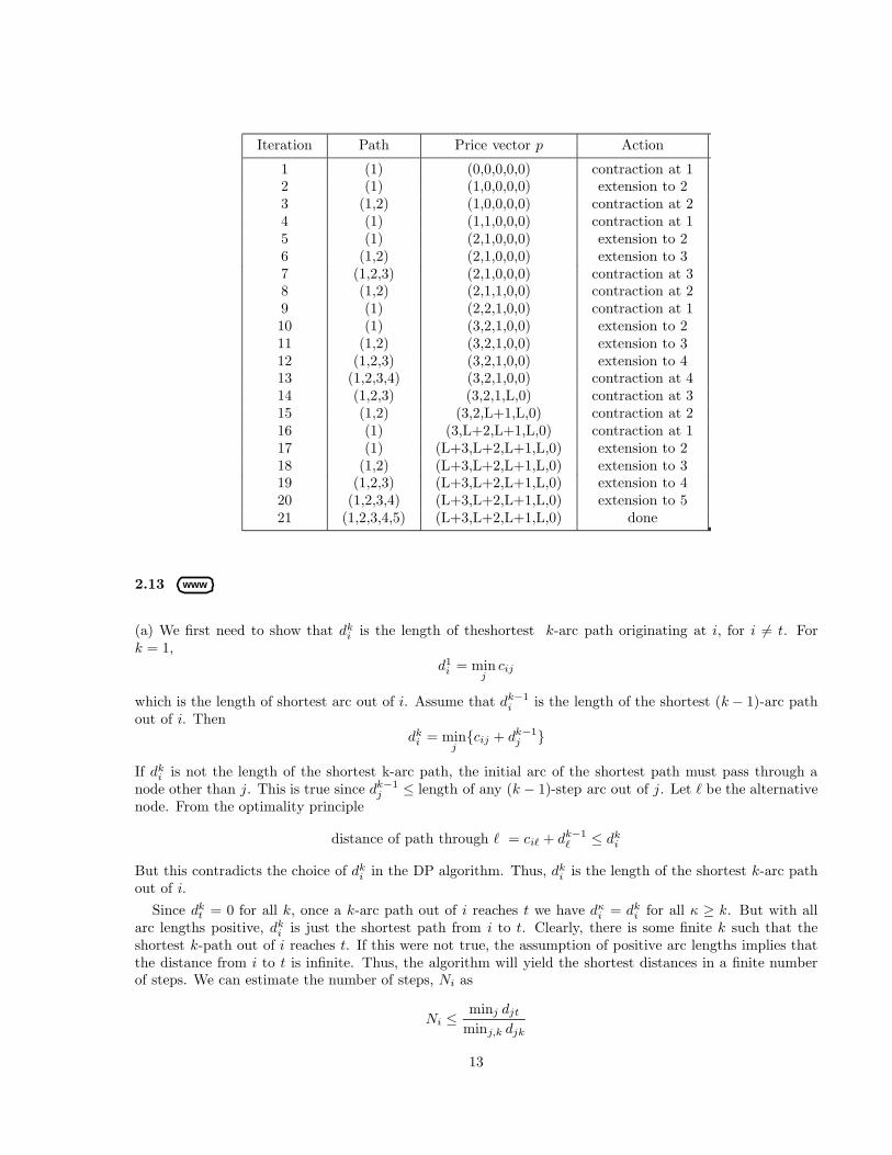
(c) The iterations of the modified algorithm applied to the problem of Exercise 2.8 are given below. The first13 iterations are the same as in the original algorithm, with the exception that at iteration 2, where the pathis extended to include node 2, arc (4,2) is also deleted. As a result of this deletion, after the contraction initeration 13, the price of node 4 is changed to L, resulting in faster convergence of the algorithm.
12
Iteration Path Price vector p Action
1 (1) (0,0,0,0,0) contraction at 12 (1) (1,0,0,0,0) extension to 23 (1,2) (1,0,0,0,0) contraction at 24 (1) (1,1,0,0,0) contraction at 15 (1) (2,1,0,0,0) extension to 26 (1,2) (2,1,0,0,0) extension to 37 (1,2,3) (2,1,0,0,0) contraction at 38 (1,2) (2,1,1,0,0) contraction at 29 (1) (2,2,1,0,0) contraction at 110 (1) (3,2,1,0,0) extension to 211 (1,2) (3,2,1,0,0) extension to 312 (1,2,3) (3,2,1,0,0) extension to 413 (1,2,3,4) (3,2,1,0,0) contraction at 414 (1,2,3) (3,2,1,L,0) contraction at 315 (1,2) (3,2,L+1,L,0) contraction at 216 (1) (3,L+2,L+1,L,0) contraction at 117 (1) (L+3,L+2,L+1,L,0) extension to 218 (1,2) (L+3,L+2,L+1,L,0) extension to 319 (1,2,3) (L+3,L+2,L+1,L,0) extension to 420 (1,2,3,4) (L+3,L+2,L+1,L,0) extension to 521 (1,2,3,4,5) (L+3,L+2,L+1,L,0) done
2.13 www
(a) We first need to show that dki is the length of the shortest k-arc path originating at i, for i 6= t. For
k = 1,d1
i = minj
cij
which is the length of shortest arc out of i. Assume that dk−1i is the length of the shortest (k − 1)-arc path
out of i. Thendk
i = minj{cij + dk−1
j }
If dki is not the length of the shortest k-arc path, the initial arc of the shortest path must pass through a
node other than j. This is true since dk−1j ≤ length of any (k − 1)-step arc out of j. Let ` be the alternative
node. From the optimality principle
distance of path through ` = ci` + dk−1` ≤ dk
i
But this contradicts the choice of dki in the DP algorithm. Thus, dk
i is the length of the shortest k-arc pathout of i.
Since dkt = 0 for all k, once a k-arc path out of i reaches t we have dκ
i = dki for all κ ≥ k. But with all
arc lengths positive, dki is just the shortest path from i to t. Clearly, there is some finite k such that the
shortest k-path out of i reaches t. If this were not true, the assumption of positive arc lengths implies thatthe distance from i to t is infinite. Thus, the algorithm will yield the shortest distances in a finite numberof steps. We can estimate the number of steps, Ni as
Ni ≤minj djt
minj,k djk
13
(b) Let dki be the distance estimate generated using the initial condition d0
i = ∞ and dki be the estimate
generated using the initial condition d0i = 0. In addition, let di be the shortest distance from i to t.
Lemmadk
i ≤ dk+1i ≤ di ≤ dk+1
i ≤ dki (1)
dki = di = dk
i for k sufficently large (2)
Proof Relation (1) follows from the monotonicity property of DP. Note that d1i ≥ d0
i and that d1i ≤ d0
i .Equation (2) follows immediately from the convergence of DP (given d0
i = ∞) and from part a).
Proposition For every k there exists a time Tk such that for all T ≥ Tk
dki ≤ dT
i ≤ dki , i = 1,2, . . . , N
Proof The proof follows by induction. For k = 0 the proposition is true, given the positive arc lengthassumption. Asume it is true for a given k. Let N (i) be a set containing all nodes adjacent to i. For everyj ∈ N(i) there exists a time, T j
k such that
dkj ≤ dT
j ≤ dkj ∀ T ≥ T j
k
Let T ′ be the first time i updates its distance estimate given that all dT j
kj , j ∈ N(i), estimates have arrived.
Let dTij be the estimate of dj that i has at time T ′. Note that this may differ from d
T jk
j since the laterestimates from j may have arrived before T ′. From the Lemma
dkj ≤ dT ′
ij ≤ dkj
which, coupled with the monotonicity of DP, implies
dk+1i ≤ dT
i ≤ dk+1i ∀ T ≥ T ′
Since each node never stops transmitting, T ′ is finite and the proposition is proved. Using the Lemma, wesee that there is a finite k such that dκ
i = di = dκi , ∀ κ ≥ k. Thus, from the proposition, there exists a finite
time T ∗ such that dTi = d∗i for all T ≥ T ∗ and i.
14
Vol. I, Chapter 3
3.6 www
This problem is similar to the Brachistochrone Problem (Example 4.2) described in the text. As in thatproblem, we introduce the system
x = u
and have a fixed terminal state problem [x(0) = a and x(T ) = b]. Letting
g(x, u) =
√1 + u2
Cx,
the Hamiltonian is
H(x, u, p) = g(x, u) + pu.
Minimization of the Hamiltonian with respect to u yields
p(t) = −∇ug(x(t), u(t)).
Since the Hamiltonian is constant along an optimal trajectory, we have
g(x(t), u(t))−∇ug(x(t), u(t))u(t) = constant.
Substituting in the expression for g, we have
√1 + u2
Cx− u2
√1 + u2Cx
=1√
1 + u2Cx= constant,
which simplifies to
(x(t))2(1 + (x(t))2) = constant.
Thus an optimal trajectory satisfies the differential equation
x(t) =
√D − (x(t))2
(x(t))2.
It can be seen through straightforward calculation that the curve
(x(t))2 + (t− d)2 = D
satisfies this differential equation, and thus the curve of minimum travel time from A to B is an arc of acircle.
15
3.9 www
We have the system x(t) = Ax(t) + Bu(t), for which we want to minimize the quadratic cost
x(T )′QT x(T ) +
∫ T
0
[x(t)′Qx(t) + u(t)′Ru(t)] dt.
The Hamiltonian here isH(x, u, p) = x′Qx + u′Ru + p′(Ax + Bu),
and the adjoint equation isp(t) = −A′p(t)− 2Qx(t),
with the terminal conditionp(T ) = 2Qx(T ).
Minimizing the Hamiltonian with respect to u yields the optimal control
u∗(t) = arg minu
[x∗(t)′Qx∗(t) + u′Ru + p′(Ax∗(t) + Bu)]
=1
2R−1B′p(t).
We now hypothesize a linear relation between x∗(t) and p(t)
2K(t)x∗(t) = p(t), ∀ t ∈ [0, T ],
and show that K(t) can be obtained by solving the Riccati equation. Substituting this value of p(t) into theprevious equation, we have
u∗(t) = −R−1B′K(t)x∗(t).
By combining this result with the system equation, we have
x(t) = (A− BR−1B′K(t))x∗(t). (∗)
Differentiating 2K(t)x∗(t) = p(t) and using the adjoint equation yields
and we thus see that K(t) should satisfy the Riccati equation
K(t) = −K(t)A− A′K(t) + K(t)BR−1B′K(t)−Q.
From the terminal condition p(T ) = 2Qx(T ), we have K(T ) = Q, from which we can solve for K(t) using theRiccati equation. Once we have K(t), we have the optimal control u∗(t) = −R−1B′K(t)x∗(t). By reversingthe previous arguments, this control can then be shown to satisfy all the conditions of the PontryaginMinimum Principle.
16
Vol. I, Chapter 4
4.10 www
(a) Clearly, JN (x) is continuous. Assume that Jk+1(x) is continuous. We have
Jk(x) = minu∈{0,1,...}
{cu + L(x + u) + G(x + u)
}
where
G(y) = Ewk
{Jk+1(y − wk)}
L(y) = Ewk
{p max(0, wk − y) + h max(0, y − wk)}
Thus, L is continuous. Since Jk+1 is continuous, G is continuous for bounded wk. Assume that Jk is notcontinuous. Then there exists a x such that as y → x, Jk(y) does not approach Jk(x). Let
uy = arg minu∈{0,1,...}
{cu + L(y + u) + G(y + u)
}
Since L and G are continuous, the discontinuity of Jk at x implies
limy→x
uy 6= ux
But since uy is optimal for y,
limy→x
{cuy + L(y + uy) + G(y + uy)
}< lim
y→x
{cux + L(y + ux) + G(y + ux)
}= Jk(x)
This contradicts the optimality of Jk(x) for x. Thus, Jk is continuous.
(b) LetYk(x) = Jk(x + 1)− Jk(x)
Clearly YN (x) is a non-decreasing function. Assume that Yk+1(x) is non-decreasing. Then
Yk(x + δ)− Yk(x) = c(ux+δ+1 − ux+δ)− c(ux+1 − ux)
+ L(x + δ + 1 + ux+δ+1)− L(x + δ + ux+δ)
− [L(x + 1 + ux+1) −L(x + ux)]
+ G(x + δ + 1 + ux+δ+1)−G(x + δ + ux+δ)
− [G(x + 1 + ux+1) −G(x + ux)]
Since Jk is continuous, uy+δ = uy for δ sufficiently small. Thus, with δ small,
Now, since the control and penalty costs are linear, the optimal order given a stock of x is less than theoptimal order given x + 1 stock plus one unit. Thus
ux+1 ≤ ux ≤ ux+1 + 1
17
If ux = ux+1 + 1, Y (x + δ)− Y (x) = 0 and we have the desired result. Assume that ux = ux+1. Since L(x)is convex, L(x + 1)−L(x) is non-decreasing. Using the assumption that Yk+1(x) is non-decreasing, we have
(c) From their definition and a straightforward induction it can be shown that J∗k (x) and Jk(x, u) are boundedbelow. Furthermore,since limx→∞ Lk(x, u) = ∞, we obtain limx→∞(x, 0) = ∞.
We show that Sk is well defined. If no Sk satisfying (1) exists, we must have either Jk(x, 0)− Jk(x + 1, 0) >c, ∀ x ∈ R or Jk(x, 0) − Jk(x + 1,0) < 0, ∀ x ∈ R, because Jk is continuous. The first possibilitycontradicts the fact that limx→∞ Jk(x, 0) = ∞. The second possibility implies that limx→ −∞ Jk(x, 0) + cxis finite. However, using the boundedness of J∗k+1(x) from below, we obtain limx→ −∞ Jk(x, 0) + cx = ∞.The contradiction shows that Sk is well defined.
We now derive the form of an optimal policy u∗k(x). Fix some x and consider first the case x ≥ Sk. Usingthe fact that Jk(x, u) − Jk(x + 1, u) is nondecreasing function of x we have for any u ∈ {0, 1,2, . . .}
Therefore,Jk(x, u + 1) = Jk(x + 1, u) + c ≥ Jk(x, u) ∀u ∈ {0, 1, . . .}, ∀ x ≥ Sk.
This shows that u = 0 minimizes Jk(x, u), for all x ≥ Sk. Now let x ∈ [Sk−n, Sk −n +1), n ∈ {1, 2, . . .}.Using (2), we have
Jk(x, n + m) − Jk(x, n) = Jk(x + n,m) − Jk(x + n, 0) ≥ 0 ∀ m in {0,1, . . .}. (3)
However, if u < n then x + u < Sk and
Jk(x + u + 1, 0)− Jk(x + u, 0) < Jk(Sk + 1,0) − Jk(Sk, 0) = −c.
Therefore,
Jk(x, u + 1) = Jk(x + u + 1, 0) + (u + 1)c < Jk(x + u, 0) + uc = Jk(x, u) ∀ u ∈ {0,1, . . .}, n < n. (4)
Inequalities (3),(4) show that u = n minimizes Jk(x, u) whenever x ∈ [Sk − n,Sk − n + 1).
18
4.18 www
Let the state xk be defined as
xk =
T, if the selection has already terminated
1, if the kth object observed has rank 1
0, if the kth object observed has rank < 1
The system evolves according to
xk+1 =
{T, if uk = stop or xk = Twk, if uk = continue
The cost function is given by
gk(xk, uk, wk) =
{kN, if xk = 1 and uk = stop0, otherwise
gN (xN ) =
{1, if xN = 10, otherwise
Note that if termination is selected at stage k and xk 6= 1 then the probability of success is 0. Thus, if xk = 0it is always optimal to continue.
To complete the model we have to determine P (wk | xk, uk)4= P (wk) when the control uk = continue.
At stage k, we have already selected k objects from a sorted set. Since we know nothing else about theseobjects the new element can, with equal probability, be in any relation with the already observed objects aj
and µ∗N−1(1) = stop. Note that N − 1 ∈ SN for all SN .
Assume the proposition is true for Jk+1(xk+1). Then
Jk(0) = max[
0︸︷︷︸stop
, E{Jk+1(wk)}︸ ︷︷ ︸continue
]
Jk(1) = max[ k
N︸︷︷︸stop
, E{Jk+1(wk)}︸ ︷︷ ︸continue
]
Now,
E{Jk+1(wk)} =1
k + 1
k + 1
N+
k
k + 1
k + 1
N
(1
N − 1+ · · ·+ 1
k + 1
)
=k
N
(1
N − 1+ · · ·+ 1
k
)
Clearly
Jk(0) =k
N
(1
N − 1+ · · ·+ 1
k
)
and µ∗k(0) = continue. If k ∈ SN ,
Jk(1) =k
N
and µ∗k(1) = stop. Q.E.D.
Proposition If k 6∈ SN
Jk(0) = Jk(1) =δ − 1
N
(1
N − 1+ · · ·+ 1
δ − 1
)
where δ is the minimum element of SN .
Proof For k = δ − 1
Jk(0) =1
δ
δ
N+
δ − 1
δ
δ
N
(1
N − 1+ · · ·+ 1
δ
)
=δ − 1
N
(1
N − 1+ · · ·+ 1
δ − 1
)
Jk(1) = max
[δ − 1
N,δ − 1
N
(1
N − 1+ · · ·+ 1
δ − 1
)]
=δ − 1
N
(1
N − 1+ · · ·+ 1
δ − 1
)
and µ∗δ−1(0) = µ∗δ−1(1) = continue.
Assume the proposition is true for Jk(xk). Then
Jk−1(0) =1
kJk(1) +
k − 1
kJk(0) = Jk(0)
20
and µ∗k−1(0) = continue.
Jk−1(1) = max
[1
kJk(1) +
k − 1
kJk(0),
k − 1
N
]
= max
[δ − 1
N
(1
N − 1+ · · ·+ 1
δ − 1
),k − 1
N
]
= Jk(0)
and µ∗k−1(1) = continue. Q.E.D.
Thus the optimum policy is to continue until the δth object, where δ is the minimum integer such that(1
N−1 + · · ·+ 1δ
)≤ 1, and then stop at the first time an element is observed with largest rank.
4.31 www
(a) In order that Akx+Bku+w ∈ X for all w ∈ Wk, it is sufficient that Akx+Bku belong to some ellipsoidX such that the vector sum of X and Wk is contained in X . The ellipsoid
X = {z | z′Fz ≤ 1},
where for some scalar β ∈ (0, 1),F−1 = (1− β)(Ψ−1 − β−1D−1
k )
has this property (based on the hint and assuming that F−1 is well-defined as a positive definite matrix).Thus, it is sufficient that x and u are such that
(Akx + Bku)′F (Akx + Bku) ≤ 1. (1)
In order that for a given x, there exists u with u′Rku ≤ 1 such that Eq. (1) is satisfied as well as
x′Ξx ≤ 1
it is sufficient that x is such that
minu∈<m
[x′Ξx + u′Rku + (Akx + Bku)′F (Akx + Bku)
]≤ 1, (2)
or by carryibf out explicitly the quadratic minimization above,
x′Kx ≤ 1,
whereK = A′k(F−1 + BkR−1
k B ′k)−1 + Ξ.
The control lawµ(x) = −(Rk + B′
kFBk)−1B′kFAkx
attains the minimum in Eq. (2) for all x, so it achieves reachability.
(b) Follows by iterative application of the results of part (a), starting with k = N − 1 and proceedingbackwards.
(c) Follows from the arguments of part (a).
21
Vol. I, Chapter 5
5.1 www
Define
yN = xN
yk = xk + A−1k wk + A−1
k A−1k+1wk+1 + . . . + A−1
k · · ·A−1N−1wN−1
Then
yk = xk + A−1k (wk − xk+1) + A−1
k yk+1
= xk + A−1k (−Akxk − Bkuk) + A−1
k yk+1
= −A−1k Bkuk + A−1
k yk+1
andyk+1 = Akyk + Bkuk
Now, the cost function is the expected value of
xN′QxN +
N−1∑
k=0
uk′Rkuk = y0
′K0y0 +
N−1∑
k=0
(yk+1′Kk+1yk+1 − yk
′Kkyk + uk′Rkuk)
We have
yk+1′Kk+1yk+1 − yk
′Kkyk + uk′Rkuk = (Akyk + Bkuk)
′Kk+1(Akyk + Bkuk) + uk
′Rkuk
− yk′Ak
′[Kk+1 −Kk+1Bk(Bk′Kk+1Bk)−1BkτrKk+1]Akyk
= yk′Ak
′Kk+1Akyk + 2y′kA′kKk+1Bkuk + uk′Bk
′Kk+1Bkuk
− yk′Ak
′Kk+1Akyk + yk′Ak
′Kk+1BkP−1k B′
kKk+1Akyk
+ uk′Rkuk
= −2y′kL′kPkuk + uk′Pkuk + yk
′Lk′PkLkyk
= (uk −Lkyk)′Pk(uk − Lkyk)
Thus, the cost function can be written as
E{
y0′K0y0 +
N−1∑
k=0
(uk − Lkyk)′Pk(uk − Lkyk)
}
The problem now is to find µ∗k(Ik), k = 0, 1, . . . , N − 1, that minimize over admissible control laws µk(Ik),k = 0, 1, . . . , N − 1, the cost function
E{
y0′K0y0 +
N−1∑
k=0
(µk(Ik)− Lkyk
)′Pk
(µk(Ik)− Lkyk
)}
22
We do this minimization by first minimizing over µN−1, then over µN−2, etc. The minimization over µN−1
involves just the last term in the sum and can be written as
minµN−1
E{(
µN−1(IN−1)− LN−1yN−1
)′PN−1
(µN−1(IN−1)− LN−1yN−1
)}
= E{
minuN−1
E{(
uN−1 − LN−1yN−1
)′PN−1
(uN−1 − LN−1yN−1
)∣∣IN−1
}}
Thus this minimization yields the optimal control law for the last stage
µ∗N−1(IN−1) = LN−1 E{yN−1
∣∣IN−1
}
(Recall here that, generically, E{z|I}minimizes over u the expression Ez{(u− z)′P (u− z)|I} for any randomvariable z, any conditioning variable I, and any positive semidefinite matrix P .) The minimization over µN−2
involves
E{(
µN−2(IN−2) −LN−2yN−2
)′PN−2
(µN−2(IN−2)− LN−2yN−2
)}
+ E{(
E{yN−1|IN−1} − yN−1
)′L′N−1PN−1LN−1
(E{yN−1|IN−1} − yN−1
)}
However, as in the lemma of p. 104, the term E{yN−1|IN−1}− yN−1 does not depend on any of the controls(it is a function of x0, w0, . . . , wN−2, v0, . . . , vN−1). Thus the minimization over µN−2 involves just the firstterm above and yields similarly as before
µ∗N−2(IN−2) = LN−2 E{yN−2
∣∣IN−2
}
Proceeding similarly, we prove that for all k
µ∗k(Ik) = Lk E{yk
∣∣Ik
}
Note : The preceding proof can be used to provide a quick proof of the separation theorem for linear-quadraticproblems in the case where x0, w0, . . . , wN−1, v0, . . . , vN−1 are independent. If the cost function is
E{
xN′QN xN +
N−1∑
k=0
(xk′Qkxk + uk
′Rkuk
)}
the preceding calculation can be modified to show that the cost function can be written as
E{
x0′K0x0 +
N−1∑
k=0
((uk − Lkxk)
′Pk(uk − Lkxk) + wk
′Kk+1wk
)}
By repeating the preceding proof we then obtain the optimal control law as
µ∗k(Ik) = Lk E{
xk
∣∣Ik
}
23
5.3 www
The control at time k is (uk, αk) where αk is a variable taking values 1 (if the next measurement at timek + 1 is of type 1) or 2 (if the next measurement is of type 2). The cost functional is
E{
xN′QxN +
N−1∑
k=0
(xk′Qxk + uk
′Ruk) +
N−1∑
k=0
gαk
}
We apply the DP algorithm for N = 2. We have from the Riccatti equation
J1(I1) = J1(z0, z1, u0, α0)
= Ex1
{x1′(A′QA + Q)x1 | I1}+ E
w1
{w′Qw}
+ minu1
{u1′(B ′QB + R)u1 + 2E{x1 | I1}′A′QBu1
}
+ min[g1, g2]
Soµ∗1(I1) = −(B ′QB + R)−1B′QA E{x1 | I1}
α∗1(I1) =
{1, if g1 ≤ g2
2, otherwise
Note that the measurement selected at k = 1 does not depend on I1. This is intuitively clear since themeasurement z2 will not be used by the controller so its selection should be based on measurement costalone and not on the basis of the quality of estimate. The situation is different once more than one stage isconsidered.
Using a simple modification of the analysis in Section 5.2 of the text, we have
J0(I0) = J0(z0)
= minu0
{E
x0,w0
{x0′Qx0 + u0
′Ru0 + Ax0 + Bu0 + w0′K0Ax0 + Bu0 + w0
∣∣ z0
}}
+ minα0
[Ez1
{Ex1
{[x1 − E{x1 | I1}]′P1[x1 − E{x1 | I1}]
∣∣ I1
} ∣∣∣ z0, u0, α0
}+ gα0
]
+ Ew1
{w1′Qw1}+ min[g1, g2]
The quantity in the second bracket is the error covariance of the estimation error (weighted by P1) and, asshown in the text, it does not depend on u0. Thus the minimization is indicated only with respect to α0 andnot u0. Because all stochastic variables are Gaussian, the quantity in the second pracket does not dependon z0. (The weighted error covariance produced by the Kalman filter is precomputable and depends only onthe system and measurement matrices and noise covariances but not on the measurements received.) In fact
Ez1
{Ex1
{[x1 − E{x1 | I1}]′P1[x1 − E{x1 | I1}]
∣∣ I1
} ∣∣∣ z0, u0, α0
}
=
Tr
(P
121
∑11|1 P
121
), if α0 = 1
Tr
(P
121
∑21|1 P
121
), if α0 = 2
where Tr(•) denotes the trace of a matrix, and∑1
1|1 (∑2
1|1) denotes the error covariance of the Kalman
filter estimate if a measurement of type 1 (type 2) is taken at k = 0. Thus at time k = 0 we have that theoptimal measurement chosen does not depend on z0 and is of type 1 if
∑ni=1 P (xk = i)P (xk+1 = j|xk = i, uk)P (zk+1|uk, xk+1 = j)∑n
s=1
∑ni=1 P (xk = i)P (xk+1 = s|xk = i, uk)P (zk+1|uk, xk+1 = s)
=
∑ni=1 pi
kpij(uk)rj(uk, zk+1)∑ns=1
∑ni=1 pi
kpis(uk)rs(uk, zk+1).
Rewriting pjk+1 in vector form, we have
pjk+1 =
P ′kP.j(uk)rj(uk, zk+1)∑ns=1 P ′kP.s(uk)rs(uk, zk+1)
=rj(uk, zk+1)[P (uk)′Pk]j∑n
s=1 rs(uk, zk+1)[P (uk)′Pk]s, j = 1, . . . , n.
Therefore,
Pk+1 =[r(uk, zk+1)] ∗ [P (uk)′Pk]
r(uk, zk+1)′P (uk)′Pk.
(b) The DP algorithm for this system is
JN−1(PN−1) = minu
n∑
i=1
piN−1
n∑
j=1
pij(u)gN−1(i, u, j)
= minu
{n∑
i=1
piN−1[GN−1(u)]i
}
= minu{P ′N−1GN−1(u)}
Jk(Pk) = minu{
n∑
i=1
pik
n∑
j=1
pij(u)gk(i, u, j) +
n∑
i=1
pik
n∑
j=1
pij(u)
q∑
θ=1
rj(u, θ)Jk+1(Pk+1|Pk, u, θ)}
= minu{P ′kGk(u) +
q∑
θ=1
r(u, θ)′P (u)′PkJk+1
[[r(u, θ)] ∗ [P (u)′Pk]
r(u, θ)′P (u)′Pk
]}.
(c) For k = N − 1,
JN−1(λP ′N−1) = minu{λP ′N−1GN−1(u)} = min
u{
n∑
i=1
λpiN−1[GN−1(u)]i} = min
u{λ
n∑
i=1
piN−1[GN−1(u)]i}
= λ minu{
n∑
i=1
piN−1[GN−1(u)]i} = λ min
u{
n∑
i=1
piN−1[GN−1(u)]i} = λJN−1(PN−1).
25
Now assume Jk(λPk) = λJk(Pk). Then,
Jk−1(λP ′k−1) = minu{λP ′k−1Gk−1(u) +
q∑
θ=1
r(u, θ)′P (u)′λPk−1Jk(Pk|Pk−1, u, θ)}
= minu{λP ′k−1Gk−1(u) + λ
q∑
θ=1
r(u, θ)′P (u)′Pk−1Jk(Pk|Pk−1, u, θ)}
= λ minu{P ′k−1Gk−1(u) +
q∑
θ=1
r(u, θ)′P (u)′Pk−1Jk(Pk|Pk−1, u, θ)}
= λJk−1(Pk−1). Q.E.D.
Note that induction is not necessary to show that Jk(λPk) = λJk(Pk).
For any u, r(u, θ)′P (u)′Pk is a constant. Therefore, letting λ = r(u, θ)′P (u)′Pk, we have
Jk(Pk) = minu{P ′kGk(u) +
q∑
θ=1
r(u, θ)′P (u)′PkJk+1
[[r(u, θ)] ∗ [P (u)′Pk]
r(u, θ)′P (u)′Pk
]}
= min
[P ′kGk(u′) +
q∑
θ=1
Jk+1([r(u, θ)] ∗ [P (u)′Pk])
].
(d) For k = N − 1, we have JN−1(PN−1) = min[P ′N−1GN−1(u)], and so JN−1(PN−1) has the desired form
JN−1(PN−1) = min[P ′N−1α
1N−1, . . . , P
′N−1α
mN−1],
where αjN−1 is the jth element of GN−1(u).
Assume Jk+1(Pk+1) = min[P ′k+1α1k+1, . . . , P
′k+1α
mk+1k+1 ]. Then, using the expression from part (c) for
JK(Pk),
Jk(Pk) = min
[P ′kGk(u′) +
q∑
θ=1
Jk+1([r(u, θ)] ∗ [P (u)′Pk])
]
= min
[P ′kGk(u) +
q∑
θ=1
min[{[r(u, θ)] ∗ [P (u)′Pk]}′αk+1]
]
= min
[P ′kGk(u) +
q∑
θ=1
min[P ′kP (u)r(u, θ)′αk+1]
]
= min
[P ′k{Gk(u) +
q∑
θ=1
min[P (u)r(u, θ)′αk+1]
]
= min[P ′kα1
k, . . . , P ′kαmkk ]
],
where
αk = Gk(u) +
q∑
θ=1
min[P (u)r(u, θ)′αk+1].
The induction is thus complete.
26
Vol. I, Chapter 6
6.8 www
First, we notice that α−β pruning is applicable only for arcs that point to right children, so that at least onesequence of moves (starting from the current position and ending at a terminal position, that is, one with nochildren) has been considered. Furthermore, due to depth-first search the score at the ancestor positions hasbeen derived without taking into account the positions that can be reached from the current point. Supposenow that α-pruning applies at a position with Black to play. Then, if the current position is reached (due toa move by White), Black can respond in such a way that the final position will be worse (for White) than itwould have been if the current position were not reached. What α-pruning saves is searching for even worsepositions (emanating from the current position). The reason for this is that White will never play so thatBlack reaches the current position, because he certainly has a better alternative. A similar argument appliesfor β pruning.
A second approach: Let us suppose that it is the WHITE’s turn to move. We shall prove that a β−cutoffoccurring at the nth position will not affect the backed up score. We have from the definition of β β =min{TBS of all ancestors of n (white) where BLACK has the move}. For a cutoff to occur: TBS(n) > β.Observe first of all that β = TBS(n1) for some ancestor n1 where BLACK has the move. Then there exists apath n1, n2, . . . , nk, n. Since it is WHITE’s move at n we have that TBS(n) = max{TBS(n), BS(ni)} > β,where ni are the descendants of n. Consider now a position nk. Then TBS(nk) will either remain unchangedor will increase to a value greater than β as a result of the exploration of node n. Proceeding similarly, weconclude that TBS(n2) will either remain the same or change to a value greater than β. Finally at node n1
we have that TBS(n1) will not change since it is BLACK’s turn to move and he will choose the move withminimum score. Thus the backed up score and the choice of the next move are unaffected from β−pruning.A similar argument holds for α−pruning.
6.12 www
(a) We have for all iF (i) ≥ F (i) = aij(i) + F
(j(i)
). (1)
Assume, in order to come to a contradiction, that the graph of the N − 1 arcs(i, j(i)
), i = 1, . . . ,N − 1,
contains a cycle (i1, i2, . . . , ik, i1). Using Eq. (1), we have
F (i1) ≥ ai1i2 + F (i2),
F (i2) ≥ ai2i3 + F (i3),
· · ·
F (ik) ≥ aiki1 + F (i1).
By adding the above inequalities, we obtain
0 ≥ ai1i2 + ai2i3 + · · ·+ aiki1 .
Thus the length of the cycle (i1, i2, . . . , ik, i1) is nonpositive, a contradiction. Hence, the graph of the N − 1arcs
(i, j(i)
), i = 1, . . . , N − 1, contains no cycle. Given any node i 6= N , we can start with arc
(i, j(i)
),
27
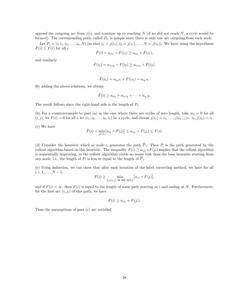
append the outgoing arc from j(i), and continue up to reaching N (if we did not reach N , a cycle would beformed). The corresponding path, called Pi, is unique since there is only one arc outgoing from each node.
Let Pi = (i, i1, i2, . . . , ik, N) [so that i1 = j(i1), i2 = j(i1), . . . , N = j(ik)]. We have using the hypothesisF (i) ≤ F (i) for all i
F (i) = aii1 + F (i1) ≥ aii1 + F (i1),
and similarlyF (i1) = ai1i2 + F (i2) ≥ ai1i2 + F (i2),
· · ·
F (ik) = aikN + F (iN ) = aikN .
By adding the above relations, we obtain
F (i) ≥ aii1 + ai1i2 + · · ·+ aikN .
The result follows since the right-hand side is the length of Pi.
(b) For a counterexample to part (a) in the case where there are cycles of zero length, take aij = 0 for all(i, j), let F (i) = 0 for all i, let (i1, i2, . . . , ik, i1) be a cycle, and choose j(i1) = i2, . . . , j(ik−1) = ik, j(ik) = i1.
(c) We haveF (i) = min
j∈Ji
[aij + F (j)
]≤ aiji + F (ji) ≤ F (i).
(d) Consider the heuristic which at node i, generates the path P i. Then Pi is the path generated by therollout algorithm based on this heuristic. The inequality F (i) ≥ aiji+F (ji) implies that the rollout algorithmis sequentially improving, so the rollout algorithm yields no worse cost than the base heuristic starting fromany node, i.e., the length of Pi is less or equal to the length of P i.
(e) Using induction, we can show that after each iteration of the label correcting method, we have for alli = 1, . . . , N − 1,
F (i) ≥ min{j|(i,j) is an arc}
[aij + F (j)
],
and if F (i) < ∞, then F (i) is equal to the length of some path starting at i and ending at N . Furthermore,for the first arc (i, ji) of this path, we have
F (i) ≥ aiji + F (ji).
Thus the assumptions of part (c) are satisfied.
28
Vol. I, Chapter 7
7.8 www
A threshold policy is specified by a threshold integer m and has the form
Process the orders if and only if their number exceeds m.
The cost function corresponding to a threshold policy specified by m will be denoted by Jm. By Prop. 3.1(c),this cost function is the unique solution of system of equations
Jm(i) =
{K + α(1− p)Jm(0) + αpJm(1) if i > m,ci + α(1− p)Jm(i) + αpJm(i + 1) if i ≤ m.
(1)
Thus for all i ≤ m, we have
Jm(i) =ci + αpJm(i + 1)
1− α(1− p),
Jm(i − 1) =c(i− 1) + αpJm(i)
1− α(1 − p).
From these two equations it follows that for all i ≤ m, we have
Jm(i) ≤ Jm(i + 1) ⇒ Jm(i − 1) < Jm(i). (2)
Denote nowγ = K + α(1− p)Jm(0) + αpJm(1).
Consider the policy iteration algorithm, and a policy µ that is the successor policy to the threshold policycorresponding to m. This policy has the form
Process the orders if and only if
K + α(1− p)Jm(0) + αpJm(1) ≤ ci + α(1− p)Jm(i) + αpJm(i + 1)
or equivalentlyγ ≤ ci + α(1− p)Jm(i) + αpJm(i + 1).
In order for this policy to be a threshold policy, we must have for all i
This relation holds if the function Jm is monotonically nondecreasing, which from Eqs. (1) and (2) will betrue if Jm(m) ≤ Jm(m + 1) = γ.
Let us assume that the opposite case holds, where γ < Jm(m). For i > m, we have Jm(i) = γ, so that
ci + α(1 − p)Jm(i) + αpJm(i + 1) = ci + αγ. (4)
We also have
Jm(m) =cm + αpγ
1− α(1− p),
from which, together with the hypothesis Jm(m) > γ, we obtain
cm + αγ > γ. (5)
29
Thus, from Eqs. (4) and (5) we have
ci + α(1− p)Jm(i) + αpJm(i + 1) > γ, for all i > m, (6)
so that Eq. (3) is satisfied for all i > m.
For i ≤ m, we have ci + α(1 − p)Jm(i) + αpJm(i + 1) = Jm(i), so that the desired relation (3) takes theform
γ ≤ Jm(i − 1) ⇒ γ ≤ Jm(i). (7)
To show that this relation holds for all i ≤ m, we argue by contradiction. Suppose that for some i ≤ m we haveJm(i) < γ ≤ Jm(i−1). Then since Jm(m) > γ, there must exist some i > i such that Jm(i−1) < Jm(i). Butthen Eq. (2) would imply that Jm(j−1) < Jm(j) for all j ≤ i, contradicting the relation Jm(i) < γ ≤ Jm(i−1)assumed earlier. Thus, Eq. (7) holds for all i ≤ m so that Eq. (3) holds for all i. The proof is complete.
7.12 www
Let Assumption 2.1 hold and let π = {µ0, µ1, . . .} be an admissible policy. Consider also the sets Sk(i) givenin the hint with S0(i) = {i}. If t ∈ Sn(i) for all π and i, we are done. Otherwise, we must have for some πand i, and some k < n, Sk(i) = Sk+1(i) while t /∈ Sk(i). For j ∈ Sk(i), let m(j) be the smallest integer msuch that j ∈ Sm. Consider a stationary policy µ with µ(j) = µm(j)(j) for all j ∈ Sk(i). For this policy wehave for all j ∈ Sk(i),
pjl(µ(j)) > 0 ⇒ l ∈ Sk(i).
This implies that the termination state t is not reachable from all states in Sk(i) under the stationary policyµ, and contradicts Assumption 2.1.