TECHNISCHE MECHANIK, Band 28, Heft 3-4, (2008), 237 – 258 Manuskripteingang: 24. Oktober 2007 Dynamic Response of Prestressed Timoshenko Beams Resting on Two-Parameter Foundation to Moving Harmonic Load Nguyen Dinh Kien The dynamic response of prestressed Timoshenko beams fully and partially resting on a two-parameter elastic foundation to a moving harmonic load is investigated by the finite element method. A beam element with shear deformation taking the effect of prestress and foundation support for the dynamic analysis is formulated in the context of the field consistent approach. Using the formulated element, the dynamic response of the beams having different boundary conditions is computed by using the direct integration Newmark method. The effects of pre- stress, foundation support, moving velocity and excitation frequency on the dynamic characteristics of the beams are studied and described in detail. The numerical results show that the effects of the axial force and the moving velocity on the dynamic response of the beams are governed by the excitation frequency. The influence of acceler- ation, partial support by the elastic foundation and the significance of the second foundation parameter are also examined and highlighted. 1 Introduction The analysis of beams on elastic foundation is one of important topics in civil engineering, and it was a subject of investigation for many decades. In his classical work, Het´ enyi (1946) has presented a number of solutions for finite and infinite beams resting on various types of elastic foundation, including the Winkler foundation, variable stiffness and continuum foundations, under static loads. To take care of the shortcomings of the Winkler foundation model, Het´ enyi himself proposed a foundation model in which the interaction among discrete Winkler springs is accomplished by incorporating an elastic beam or elastic plate, and the investigation on the beams resting on the Het´ enyi foundation was also described. It is well known that the mechanical characteristics such as the displacement and the stress of a structure subjected to moving loads are quite different from those obtained by a static analysis of the structure subjected to the same loads. The displacement and the stress of the structure in a dynamic analysis depend not only on the magnitude of external loads, but also on the velocity and frequency of the loads. The dynamic analysis of beams under moving loads plays an important role in the field of railway and bridge engineering, and this topic has attracted much attention from researchers for many years. The early work on the topic has been described by Timoshenko et al. (1974), where the governing equation for a uniform Bernoulli beam subjected to a moving harmonic force with constant velocity was solved by the mode superposition method. Fryba (1972) presented a solution for the vibrations of a simply supported beam under moving loads and axial forces. Employing the traditional plane Bernoulli beam element, Thambiratnam and Zhuge (1996) performed a dynamic analysis of beams resting on a Winkler elastic foundation subjected to moving loads by the finite element method. Chen et al. (2001) investigated the response of an infinite Timoshenko beam on a viscoelastic foundation to a moving harmonic load by deriving the dynamic stiffness matrix for the beam. The natural frequencies and mode shapes of Bernoulli-type beams subjected to moving loads with variable velocity have been investigated by Dugush and Eisengerger (2002) by both the modal and direct integration methods. Using the Fourier transform method, Kim (2004) obtained the steady-state response to moving loads of axial loaded beams resting on a Winkler elastic foundation. Adopting polynomials as trial function for the deflection in the Lagrangian equations, Kocat¨ urk and S ¸ ims ¸ek (2006) investigated the vibration of viscoelastic beams subjected to an eccentric compressive force and a moving harmonic force. The objective of this paper is to investigate the dynamic response of prestressed Timoshenko beams resting on a two-parameter elastic foundation to a moving concentrated harmonic load by the finite element method. The 237
Transcript
TECHNISCHE MECHANIK, Band 28, Heft 3-4, (2008), 237 – 258Manuskripteingang: 24. Oktober 2007
Dynamic Response of Prestressed Timoshenko Beams Resting onTwo-Parameter Foundation to Moving Harmonic Load
Nguyen Dinh Kien
The dynamic response of prestressed Timoshenko beams fully and partially resting on a two-parameter elasticfoundation to a moving harmonic load is investigated by the finite element method. A beam element with sheardeformation taking the effect of prestress and foundation support for the dynamic analysis is formulated in thecontext of the field consistent approach. Using the formulated element, the dynamic response of the beams havingdifferent boundary conditions is computed by using the direct integration Newmark method. The effects of pre-stress, foundation support, moving velocity and excitation frequency on the dynamic characteristics of the beamsare studied and described in detail. The numerical results show that the effects of the axial force and the movingvelocity on the dynamic response of the beams are governed by the excitation frequency. The influence of acceler-ation, partial support by the elastic foundation and the significance of the second foundation parameter are alsoexamined and highlighted.
1 Introduction
The analysis of beams on elastic foundation is one of important topics in civil engineering, and it was a subjectof investigation for many decades. In his classical work, Hetenyi (1946) has presented a number of solutions forfinite and infinite beams resting on various types of elastic foundation, including the Winkler foundation, variablestiffness and continuum foundations, under static loads. To take care of the shortcomings of the Winkler foundationmodel, Hetenyi himself proposed a foundation model in which the interaction among discrete Winkler springs isaccomplished by incorporating an elastic beam or elastic plate, and the investigation on the beams resting on theHetenyi foundation was also described.
It is well known that the mechanical characteristics such as the displacement and the stress of a structure subjectedto moving loads are quite different from those obtained by a static analysis of the structure subjected to the sameloads. The displacement and the stress of the structure in a dynamic analysis depend not only on the magnitude ofexternal loads, but also on the velocity and frequency of the loads.
The dynamic analysis of beams under moving loads plays an important role in the field of railway and bridgeengineering, and this topic has attracted much attention from researchers for many years. The early work on thetopic has been described by Timoshenko et al. (1974), where the governing equation for a uniform Bernoulli beamsubjected to a moving harmonic force with constant velocity was solved by the mode superposition method. Fryba(1972) presented a solution for the vibrations of a simply supported beam under moving loads and axial forces.Employing the traditional plane Bernoulli beam element, Thambiratnam and Zhuge (1996) performed a dynamicanalysis of beams resting on a Winkler elastic foundation subjected to moving loads by the finite element method.Chen et al. (2001) investigated the response of an infinite Timoshenko beam on a viscoelastic foundation to amoving harmonic load by deriving the dynamic stiffness matrix for the beam. The natural frequencies and modeshapes of Bernoulli-type beams subjected to moving loads with variable velocity have been investigated by Dugushand Eisengerger (2002) by both the modal and direct integration methods. Using the Fourier transform method,Kim (2004) obtained the steady-state response to moving loads of axial loaded beams resting on a Winkler elasticfoundation. Adopting polynomials as trial function for the deflection in the Lagrangian equations, Kocaturk andSimsek (2006) investigated the vibration of viscoelastic beams subjected to an eccentric compressive force and amoving harmonic force.
The objective of this paper is to investigate the dynamic response of prestressed Timoshenko beams resting ona two-parameter elastic foundation to a moving concentrated harmonic load by the finite element method. The
237
prestress is assumed to result from the initial loading by axial forces, and the variation of the moving velocityis also taken into consideration. Regarding the above cited references, two different features are included inthe present work. Firstly, the shear deformation is introduced through a finite element formulation. Secondly,a two-parameter foundation model is adopted, which takes into account the interaction between springs of thetraditional Winkler foundation through the introduction of a shear layer connecting the ends of Winkler springsto a beam. Different from the Hetenyi foundation, the introduced shear layer in the two-parameter foundationmodel undergoes transverse shear deformations only, and this feature guarantees a simple mathematical form ofthe model, Dutta and Roy (2002). The accuracy and advantages of the two-parameter foundation in modelling theeffect of elastic foundation support on structures has been investigated and described by Feng and Cook (1983).
Following this introduction, the paper is organized as follows. A beam element based on the field consistentapproach for the dynamic analysis is formulated in Section 2. Section 3 describes the governing equations for thediscrete beam under a moving load. The effects of prestress, foundation support, moving velocity as well as theexcitation frequency on the dynamic response of the beams are numerically investigated in detail in Section 4. Themain conclusions of the paper are summarized in Section 5.
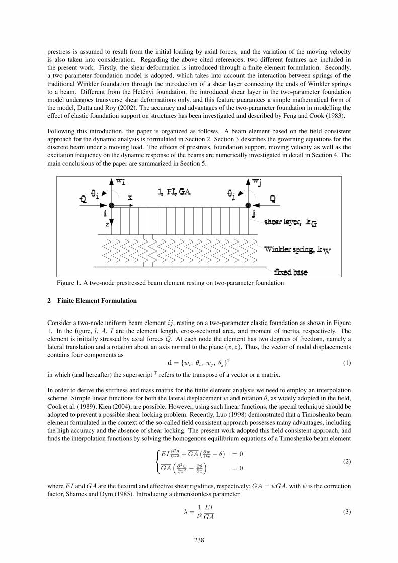
Figure 1. A two-node prestressed beam element resting on two-parameter foundation
2 Finite Element Formulation
Consider a two-node uniform beam element ij, resting on a two-parameter elastic foundation as shown in Figure1. In the figure, l, A, I are the element length, cross-sectional area, and moment of inertia, respectively. Theelement is initially stressed by axial forces Q. At each node the element has two degrees of freedom, namely alateral translation and a rotation about an axis normal to the plane (x, z). Thus, the vector of nodal displacementscontains four components as
d = wi, θi, wj , θjT (1)
in which (and hereafter) the superscript T refers to the transpose of a vector or a matrix.
In order to derive the stiffness and mass matrix for the finite element analysis we need to employ an interpolationscheme. Simple linear functions for both the lateral displacement w and rotation θ, as widely adopted in the field,Cook et al. (1989); Kien (2004), are possible. However, using such linear functions, the special technique should beadopted to prevent a possible shear locking problem. Recently, Luo (1998) demonstrated that a Timoshenko beamelement formulated in the context of the so-called field consistent approach possesses many advantages, includingthe high accuracy and the absence of shear locking. The present work adopted this field consistent approach, andfinds the interpolation functions by solving the homogenous equilibrium equations of a Timoshenko beam element
EI ∂2θ∂x2 + GA
(∂w∂x − θ
)= 0
GA(
∂2w∂x2 − ∂θ
∂x
)= 0
(2)
where EI and GA are the flexural and effective shear rigidities, respectively; GA = ψGA, with ψ is the correctionfactor, Shames and Dym (1985). Introducing a dimensionless parameter
λ =1l2
EI
GA(3)
238
we can rewrite equation (2) in the form
EI ∂2θ∂x2 + 1
λl2 EI(
∂w∂x − θ
)= 0
1λl2 EI
(∂2w∂x2 − ∂θ
∂x
)= 0
(4)
Using the command dsolve in the symbolic software Maple (1991), we can easily obtain the general solutionsfor the system of equations (4) as
w(x) = 16C1x
3 + 12C2x
2 + C3x + C4
θ(x) = C1λl2 + 12C1x
2 + C2x + C3
(5)
where the constant C1, ..., C4 are determined from element end conditions
w|x=0 = wi ; θ|x=0 = θi
w|x=l = wj ; θ|x=l = θj
(6)
Expressing the displacement and the rotation in the forms
w(x) = Nw1wi + Nw2θi + Nw3wj + Nw4θj = NTwd
θ(x) = Nθ1wi + Nθ2θi + Nθ3wj + Nθ4θj = NTθd
(7)
where Nw = Nw1, Nw2, Nw3, Nw4T and Nθ = Nθ1, Nθ2, Nθ3, Nθ4T are the vectors of interpolationfunctions for w(x) and θ(x), respectively. From equations (5)-(7), we can obtain the expressions for Nwi andNθi, (i = 1..4). The detail of these expressions are given by equations (25) and (26) in the Appendix. It can beseen from equation (25) that in the limit as GA → ∞, the interpolation functions Nwi go back to the Hermitianpolynomials which are employed in developing the traditional Bernoulli beam element, Cook et al. (1989). Inthis case, the element goes back to the traditional Bernoulli beam element, which has ability in modelling slenderbeams.
Having the interpolation functions derived, the stiffness and the consistent mass matrices for the beam elementcan be developed from strain energy and kinetic energy expressions. The strain energy of the element is stemmingfrom the beam bending, the foundation deformation and the prestress due to the axial force Q
U = UB + UF + UQ (8)
in which the strain energy for a Timoshenko beam element with length of l is given by (Shames and Dym, 1985)
UB =12
∫ l
0
[EI
(∂θ
∂x
)2
+ GA
(∂w
∂x− θ
)2]
dx (9)
The strain energy stored in the elastic foundation during the beam deformation is resulted from stretching of theWinkler springs and deformation of the shear layer as (Rao, 2003; Yokoyama, 1996)
UF =12
∫ l
0
kW w2dx +12
∫ l
0
kG
(∂w
∂x
)2
dx (10)
where kW is the Winkler foundation modulus, having units force per length2 (N/m2), and kG with dimensions offorce (N) is the stiffness of the shear layer. The geometric strain energy stemming from the prestressed effect ofthe axial force is given by (Geradin and Rixen, 1997)
UQ =12
∫ l
0
Q
(∂w
∂x
)2
dx (11)
where Q (with units N) is positive in tension. From equations (7), (25) and (26) we can easily express the strainenergy U defined by equation (8) in terms of the nodal displacements, e.g. the strain energy UB has the form
UB =2
(1 + 12λ)2l3EI
[3(wi − wj)2 + 3l(wi − wj)(θi + θj) + l2(θ2
i + θiθj + θ2j )
+ 6λl2(1 + 6λ)(θi − θj)2]+ 9λ
[2(wi − wj) + l(θi + θj)
]2 (12)
239
The expressions similar to equation (12) for UF and UQ can also easily be obtained. Finally, we can computethe element stiffness matrix as a summation of the stiffness matrices due to the beam bending, the foundationdeformation and the prestress as
k = kB + kF + kQ (13)
where
kB =∂2UB
∂d2; kF =
∂2UF
∂d2; kQ =
∂2UQ
∂d2(14)
The detail expressions for kB , kF and kQ are given by equations (27)-(31) in the Appendix. It is noted thatwhen λ approaches to zero, the stiffness matrices kB and kQ deduce exactly to the stiffness matrix of the tradi-tional Bernoulli beam element and the geometrical stiffness matrix, which employed the Hermitian polynomialsas interpolation functions, Cook et al. (1989); Geradin and Rixen (1997).
The element consistent mass matrix for the dynamic analysis can be obtained from the kinetic energy using thesame interpolation functions Nwi and Nθi (i = 1..4) for the displacement field, equations (25)-(26). To this end,we start from the kinematic energy expression, which for the Timoshenko beam element of the present work hasthe form (Geradin and Rixen, 1997)
T =12
∫ l
0
ρAw2dx +12
∫ l
0
ρIθ2dx (15)
where ρ is the mass density, and w = ∂w/∂t, θ = ∂θ/∂t. Using equation (7), we can write the kinetic energy inthe form
T =12dT
∫ l
0
ρANTwNwdxd +
12dT
∫ l
0
ρINTθNθdxd
= dTmwd + dTmθd = dTmd(16)
with
m = mw + mθ =12
∫ l
0
ρANTwNwdx +
12
∫ l
0
ρINTθNθdx (17)
is the consistent mass matrix of the element. The detail expression for mw and mθ are given by equations (32)and (33) in the Appendix. Again, in the limit as λ → 0 the mass matrix mw deduces exactly to the consistent massmatrix of the traditional Bernoulli beam element as presented by Geradin and Rixen (1997).
Figure 2. A prestressed beam resting on a two-parameter elastic foundation subjected to a moving har-monic load F = P cos(Ωt).
3 Governing Equations
Consider a prestressed beam resting on the two-parameter foundation with a moving concentrated harmonic load,F = P cos(Ωt), travelling along the beam from left to right as shown in Figure 2. In the figure, L is the total beamlength, and xF is the distance from the left end of the beam to the current moving load position. Assuming thatat time t = 0 the load F is at the left-hand support and has a velocity of vo, it then travels to the right, and at theright-hand support its velocity is vf . Following the standard procedure of the finite element method, the beam isdiscretized into a number of finite elements. The equations of motion of the beam in terms of the finite elementanalysis when ignoring the damping effect can be written in the form (Cook et al., 1989)
MD + KD = P cos(Ωt)N (18)
240
where M and K are the structural mass and stiffness matrices, respectively. These matrices are obtained byassembling the element matrices m and k formulated in Section 2 in the standard way of the finite element method;D and D = ∂2D/∂t2 are the vectors of structural nodal displacements and accelerations, respectively; N is thevector of shape functions for the beam, and having the form
where Nw1, Nw2, Nw3, Nw4 are defined by equation (25), in which the abscissa x is measured from the left-handnode of the current loading element to the position of the moving load, and for the case of equal-element mesh,this abscissa is calculated as
x = xF − (n− 1)l =vf − vo
2∆tt2 + vot− (n− 1)l (20)
with l, as before, is the element length, and n denotes the number of the element on which the load is acting (seeFigure 2); t is the current time, and ∆t is the total time needed for the load to move completely from the left-handsupport to the right-hand support.
The system of equation (18) is solved by the direct integration Newmark method using the average constant accel-eration formula, which ensures an unconditional numerical stability, Geradin and Rixen (1997).
4 Numerical Investigations
Using the finite element formulated in Section 2 and the numerical algorithm described in Section 3, a computercode was developed and used in the dynamic analysis. To investigate the dynamic response, the beam with thefollowing geometry and material data, previously employed by Kocaturk and Simsek (2006), is adopted herewith
L = 20 m; I = 0.08824 m4; ρA = 1000 kg/m; EI = 3× 10⁹ Nm2, ν = 0.3
where, in addition to the previous notations, ν denotes the Poisson ratio. The amplitude of the moving load is takenas P = 100 kN.
Figure 3. Beams for numerical investigation
Two types of boundary conditions, namely simply supported (SS) and clamped at one end and simply supportedat the other (CS) as respectively shown in Figure 3(a) and Figure 3(b) are considered. The effect of partial supportby the elastic foundation is examined by assuming that the beams are supported on a part αL, with 0 ≤ α < 1,from the left-hand end as typically depicted in Figure 3(c) for the SS beam. For the convenience of discussion, αis called the supporting parameter.
The computation in this Section is performed with a mesh of 20 equal elements, and the correction factor ψ istaken by ψ = 10(1+ν)
(12+11ν) .
241
(k1, k2) r µ Naidu and Rao (k1, k2) r µ Naidu and Rao(1995) (1995)
Table 1: Frequency parameter of the SS beam fully supported by the elastic foundation at various values of thecompressive axial force and the foundation parameters
4.1 Model Verification
This subsection aims to verify the accuracy of the formulated element and the described numerical algorithm. Tothis end, the eigenfrequency and the dynamic response of the SS beam is computed and compared to the publishedones. Following the work of Naidu and Rao (1995), we introduce herewith the dimensionless parameters k1 andk2 representing the stiffness of the Winkler springs and the shear layer of the foundation
k1 =L4
EIkW ; k2 =
L2
π2EIkG (21)
and a dimensionless parameter representing the axial force
f =L2
EIQ (22)
Furthermore, we also introduce the frequency parameter defined as
µ =(
ρAL4
EIω2
1
)1/4
(23)
with ω1 (rad/s) is the fundamental frequency (the first natural frequency) of the beams.
Table 4.1 lists the frequency parameter of the SS beam fully supported by the elastic foundation at various valuesof the compressive axial force and the foundation parameters. In the table, r = f/fb is the ratio of the axial loadparameter f , defined by equation (22), and the buckling load parameter fb corresponding to the Euler bucklingload Qb, which can be obtained by solving the eigenvalue problem
(KB + KF −QbKQ)D = 0 (24)
where KB , KF and KQ are the structural stiffness matrices, obtained by assembling the previous formulatedelement matrices kB , kF , kQ in the standard way of the finite element method, respectively. It is noted that bywriting the eigenvalue problem in the form (24), the axial force Q should be omitted from KQ.
It is seen from Table 4.1 that regardless of the axial force and the foundation stiffness, the frequency parameter ofthe SS beam fully resting on the elastic foundation obtained in the present work is in good agreement with thatreported by Naidu and Rao (1995), who computed the frequency parameter by using the traditional Bernoulli beamelements. It is necessary to note that the beam with the above geometry data is quite slender, so that the frequenciesare hardly affected by the shear deformation.
242
0 2 4 6 8 10 12 14 16 18 200
1
2
3
4
5
6x 10
−3
w (
m)
XF (m)
present work
Timoshenko et al. (1974)
(a)
0 2 4 6 8 10 12 14 16 18 20−0.06
−0.04
−0.02
0
0.02
0.04
0.06
XF (m)
w (
m)
present work
Timoshenko et al. (1974)
(b)
Figure 4. Deflection under a moving load of the SS beam without foundation support and axial force forthe case of a constant velocity v = 15 m/s and with different excitation frequencies: (a) Ω = 0rad/s, (b) Ω = 40 rad/s.
Figure 4 shows the deflection of the SS beam without the foundation support and the axial force under a constantspeed moving load and with the excitation frequency of 0 and 40 rad/s. For the purpose of calibration, the analyticalsolution presented by Timoshenko et al. (1974) is also depicted in the figure. The deflections in the figure hereand afterwards are computed at the load point. As seen from Figure 4, the deflections obtained by the numericalmethod in the present work are in excellent agrement with the results using the mode superposition method byTimoshenko et al. (1974) in the case of the moving load (Ω = 0), and in the case of the moving harmonic load(Ω = 40 rad/s). It is noted that the excitation frequency Ω = 40 rad/s employed in the analysis is very near the
243
fundamental frequency of the SS beam (ω1 = 42.5509 rad/s, see Table 4.1), so that the deflection of the beamshown in Figure 4(b) is much larger than that of Figure 4(a) due to the resonance effect. The numerical resultsshow the accuracy of the formulated element and the numerical algorithm in computing the dynamic response ofthe beam.
4.2 Effect of compressive axial force
0 2 4 6 8 10 12 14 16 18 200
0.002
0.004
0.006
0.008
0.01
w (
m)
XF (m)
axial force Q:
0.01Qb
0.1Qb
0.4Qb
(a)
0 2 4 6 8 10 12 14 16 18 20−0.02
−0.01
0
0.01
0.02
w (
m)
XF (m)
axial force Q:
0.4Qb
0.1Qb
0.01Qb
(b)
Figure 5. Effect of compressive axial force on the dynamic response of the SS beam without foundationsupport for the case of constant velocity v = 15 m/s and different excitation frequencies: (a)Ω = 0 rad/s, (b) Ω = 20 rad/s.
244
0 2 4 6 8 10 12 14 16 18 20−0.08
−0.06
−0.04
−0.02
0
0.02
0.04
0.06
0.08axial force Q:
0.01Qb
0.1Qb
0.4Qb
w (
m)
XF (m)
(a)
0 2 4 6 8 10 12 14 16 18 20−8
−6
−4
−2
0
2
4
6
8x 10
−3
w (
m)
XF (m)
axial force Q:
0.01Qb
0.1Qb
0.4Qb
(b)
Figure 6. Effect of compressive axial force on the dynamic response of the SS beam without foundationsupport for the case of constant velocity v = 15 m/s and different excitation frequencies: (a)Ω = 40 rad/s, (b) Ω = 60 rad/s.
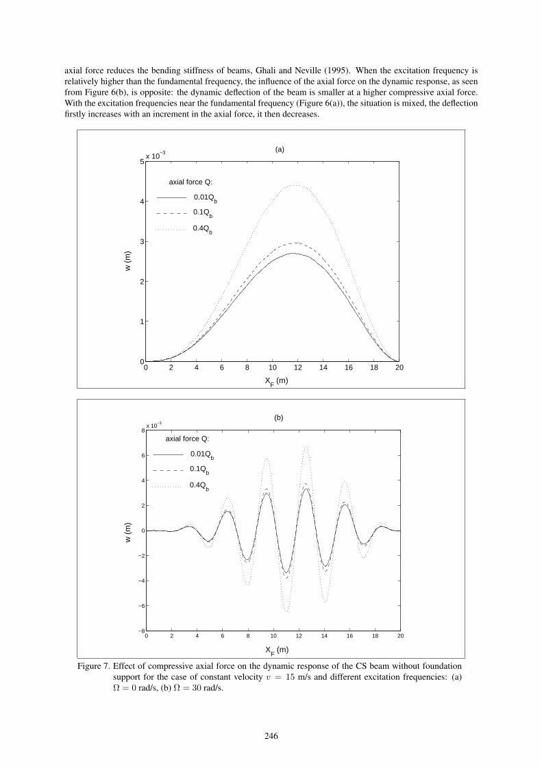
The effect of the compressive axial force on the dynamic response of the SS beam without foundation support forthe case of constant velocity v = 15 m/s and different excitation frequencies is depicted in Figure 5 and Figure 6.In the figures, Qb, as mentioned above is the Euler buckling load of the beam. As seen from the figures, the effectof the axial force depends on the the excitation frequencies, and with the excitation frequencies are considerablybelow the fundamental frequency or zero, the dynamic deflection of the beam is larger for a higher compressiveaxial force (see Figure 5). This numerical result is in agreement with the static analysis, in which the compressive
245
axial force reduces the bending stiffness of beams, Ghali and Neville (1995). When the excitation frequency isrelatively higher than the fundamental frequency, the influence of the axial force on the dynamic response, as seenfrom Figure 6(b), is opposite: the dynamic deflection of the beam is smaller at a higher compressive axial force.With the excitation frequencies near the fundamental frequency (Figure 6(a)), the situation is mixed, the deflectionfirstly increases with an increment in the axial force, it then decreases.
0 2 4 6 8 10 12 14 16 18 200
1
2
3
4
5x 10
−3
w (
m)
XF (m)
axial force Q:
0.01Qb
0.1Qb
0.4Qb
(a)
0 2 4 6 8 10 12 14 16 18 20−8
−6
−4
−2
0
2
4
6
8x 10
−3
w (
m)
XF (m)
axial force Q:
0.01Qb
0.1Qb
0.4Qb
(b)
Figure 7. Effect of compressive axial force on the dynamic response of the CS beam without foundationsupport for the case of constant velocity v = 15 m/s and different excitation frequencies: (a)Ω = 0 rad/s, (b) Ω = 30 rad/s.
246
0 2 4 6 8 10 12 14 16 18 20−0.04
−0.03
−0.02
−0.01
0
0.01
0.02
0.03
0.04
w (
m)
XF (m)
axial force Q:
0.4Qb
0.1Qb
0.01Qb
(a)
0 2 4 6 8 10 12 14 16 18 20−6
−4
−2
0
2
4
6x 10
−3
w (
m)
XF (m)
axial force Q:
0.01Qb
0.1Qb
0.4Qb
(b)
Figure 8. Effect of compressive axial force on the dynamic response of the CS beam without foundationsupport for the case of constant velocity v = 15 m/s and different excitation frequencies: (a)Ω = 60 rad/s, (b) Ω = 80 rad/s.
The above remark on the effect of the axial force, as seen from Figure 7 and Figure 8, is the same for the CS beam.It is noted that the effect of the axial force obtained in the present work is different from that reported by Kocaturkand Simsek (2006), who concluded that this effect is very small and can be ignored. The reason of this differencemay be of that the largest axial force employed by Kocaturk and Simsek is too small, just less than 3% of thebuckling load, and the effect is hardly recognized.
The effect of the compressive axial force on the dynamic response of the SS and CS beams resting on the two-
247
parameter foundation is depicted in Figure 9 and Figure 10, respectively. The numerical results shown in thefigures are obtained with k1 = 100 and k2 = 1, and in this case the fundamental frequency of the SS and CSbeams is 74.1899 rad/s and 91.2939 rad/s, respectively (see Table 4.1 for the SS beam. The natural frequency ofthe CS beam is not shown herein). The effect is almost the same as that of the case without the foundation support.In addition to the higher frequency, the deflections of the beams with the foundation support are much lower sincethe structures become much stiffer with the presence of the foundation.
0 2 4 6 8 10 12 14 16 18 20−8
−6
−4
−2
0
2
4
6
8x 10
−3
axial force Q:
0.4Qb
0.1Qb
0.01Qb
w (
m)
XF (m)
(a)
0 2 4 6 8 10 12 14 16 18 20−5
−4
−3
−2
−1
0
1
2
3
4
5x 10
−3
w (
m)
XF (m)
axial force Q:
0.4Qb
0.1Qb
0.01Qb
(b)
Figure 9. Effect of compressive axial force on the dynamic response of the SS beam resting on the two-parameter elastic foundation for the case of constant velocity v = 15 m/s and different excitationfrequencies: (a) Ω = 40 rad/s, (b) Ω = 90 rad/s (k1 = 100, k2 = 1).
248
0 2 4 6 8 10 12 14 16 18 20−8
−6
−4
−2
0
2
4
6
8x 10
−3
w (
m)
axial force Q:
0.4Qb
0.1Qb
0.01Qb
XF (m)
(a)
0 2 4 6 8 10 12 14 16 18 20−3
−2
−1
0
1
2
3x 10
−3
w (
m)
XF (m)
axial force Q:
0.01Qb
0.1Qb
0.4Qb
(b)
Figure 10. Effect of compressive axial force on the dynamic response of the CS beam resting on the two-parameter elastic foundation for the case of constant velocity v = 15 m/s and different excitationfrequencies: (a) Ω = 60 rad/s, (b) Ω = 110 rad/s (k1 = 100, k2 = 1).
4.3 Effect of moving velocity and acceleration
To investigate the effect of the moving velocity on the dynamic response of the beams, the axial force and thefoundation stiffness are kept to be constant, namely Q = 0.2Qb and (k1, k2) = (100, 1). The fundamentalfrequency of the beams in this case is 66.3570 rad/s for the SS beam, and 82.0219 rad/s for the CS beam. Thecomputation is performed with various values of the constant velocity, v = 20, 40, 60, 100 m/s, and with excitation
249
frequencies near and far from the fundamental frequencies.
0 2 4 6 8 10 12 14 16 18 20−6
−4
−2
0
2
4
6x 10
−3
velocity (m/s):
20
40
60
100
w (
m)
XF (m)
(a)
0 2 4 6 8 10 12 14 16 18 20−0.02
−0.01
0
0.01
0.02
XF (m)
w (
m)
velocity (m/s):
20
40
60
100
(b)
Figure 11. Effect of moving velocity on the dynamic response of the prestressed SS beam resting on thetwo-parameter elastic foundation with different excitation frequencies: (a) Ω = 40 rad/s, (b)Ω = 60 rad/s (Q = 0.2Qb, k1 = 100, k2 = 1).
Figure 11 shows the effect of the moving velocity on the dynamic response of the prestressed SS beam resting onthe two-parameter elastic foundation. The corresponding effect for the CS beam is depicted in Figure 12. Again,the effect of the moving velocity on the dynamic response is governed by the excitation frequencies. For theexcitation frequency well below the fundamental frequencies, the dynamic deflection of the beams firstly increaseswith an increment in the moving velocity, it then decreases, regardless of the boundary conditions (Figure 11(a)
250
and Figure 12(a)). In other words, at a given axial force and foundation stiffness, there is a critical velocity atwhich the dynamic deflection reaches a maximum value for the case of excitation frequencies much different fromthe fundamental frequencies. On the contrary, the deflections of the beams are gradually decreased in raising thevelocity when the excitation frequencies are near the fundamental frequencies (Figures 11(b) and 12(b)).
0 2 4 6 8 10 12 14 16 18 20−6
−4
−2
0
2
4
6x 10
−3
w (
m)
XF (m)
velocity (m/s):
100
60
40
20
(a)
0 2 4 6 8 10 12 14 16 18 20−0.03
−0.02
−0.01
0
0.01
0.02
0.03
w (
m)
velocity (m/s):
100
60
40
20
XF (m)
(b)
Figure 12. Effect of moving velocity on the dynamic response of the prestressed CS beam resting on thetwo-parameter elastic foundation with different excitation frequencies: (a) Ω = 60 rad/s, (b)Ω = 80 rad/s (Q = 0.2Qb, k1 = 100, k2 = 1).
The acceleration of the moving load can be defined by the difference between the velocity of the moving load atthe left-hand and right-hand ends of the beams, vo and vf , and in order to examine the effect of the accelerated
251
phenomenon, in addition to the above-mentioned parameters relating the axial force and the foundation stiffness,the moving velocity at the left-hand end of the beams is kept to be constant vo = 15 m/s, and the computation isperformed with different values of vf , namely 20, 30, 40 and 50 m/s.
0 2 4 6 8 10 12 14 16 18 20−4
−3
−2
−1
0
1
2
3
4x 10
−3w
(m
)
XF (m)
20
30
40
50
vf (m/s):
Figure 13. Effect of acceleration on the dynamic response of the prestressed SS beam resting on the two-parameter elastic foundation with an excitation frequency Ω = 40 rad/s (vo = 15 m/s, Q =0.2Qb, k1 = 100, k2 = 1).
0 2 4 6 8 10 12 14 16 18 20−4
−3
−2
−1
0
1
2
3
4x 10
−3
w (
m)
XF (m)
vf (m/s):
50
40
30
20
Figure 14. Effect of acceleration on the dynamic response of the prestressed CS beam resting on the two-parameter elastic foundation with an excitation frequency Ω = 60 rad/s (vo = 15 m/s, Q =0.2Qb, k1 = 100, k2 = 1).
252
Figures 13 and 14 show the effect of the acceleration on the dynamic response of the SS and CS beams, respectively.The curves in the figures are obtained for the excitation frequencies well below the fundamental frequencies. Asseen from the figures, the dynamic response of the beams is somehow affected by the acceleration. At the givenaxial force, the foundation stiffness and the excitation frequency, the maximum dynamic deflection increases withan increment in the acceleration, it then reaches a maximum value.
0 2 4 6 8 10 12 14 16 18 20−8
−6
−4
−2
0
2
4
6
8x 10
−3
0.8
0.6
0.4
0.2
α:
XF (m)
w (
m)
Figure 15. Effect of partial support by the elastic foundation on the dynamic response of the prestressed SSbeam to the moving load (v = 15 m/s, Ω = 20 rad/s, Q = 0.2Qb, k1 = 100 andk2 = 1).
0 2 4 6 8 10 12 14 16 18 20−6
−4
−2
0
2
4
6x 10
−3
α:
0.8
0.6
0.4
0.2
XF (m)
w (
m)
Figure 16. Effect of partial support by the elastic foundation on the dynamic response of the prestressed CSbeam to the moving load (v = 15 m/s, Ω = 40 rad/s, Q = 0.2Qb, k1 = 100 and k2 = 1).
253
020
4060
8010010
20
40
60
80
1000
0.005
0.01
0.015
k1
v (m/s)
w (
m)
(a)
020
4060
8010010
20
40
60
80
1000
0.005
0.01
k1v (m/s)
w (
m)
(b)
Figure 17. Moving velocity and foundation stiffness versus the maximum dynamic deflection of the pre-stress SS beam with an excitation frequency Ω = 20 rad/s and different values of second foun-dation parameter: (a) k2 = 0, (b) k2 = 0.5, (Q = 0.2Qb).
4.4 Effect of partial support
The effect of the partial support by the elastic foundation on the dynamic response of the prestressed SS andCS beams to the moving harmonic load is shown in Figure 15 and Figure 16, respectively. The curves shownin the figures are obtained for the case of the constant moving velocity, and with the excitation frequencies wellbelow the fundamental frequencies of the beams. Only amplitude of the dynamic deflection is affected by thepartial support, and it is lowered at a higher supporting parameter α, regardless of the boundary conditions. Thecomputation has also been performed for other excitation frequencies, but the result is very much similar to that ofthe above-mentioned frequencies, and it is not shown herein.
254
4.5 Maximum dynamic deflection
As seen from Subsection 4.3, for a given foundation, there is a value of the moving velocity at which the dynamicdeflection of the beams reaches a maximum value. This subsection investigates the influence of the moving velocityand the foundation stiffness on the maximum dynamic deflection of the beams. The maximum dynamic deflectionis defined herein as the largest amplitude of the deflection when the load completely travels from the left-hand tothe right-hand supports.
Figure 17 shows the moving velocity and the foundation stiffness versus the maximum dynamic deflection of theprestress SS beam for the case of an excitation frequency Ω = 20 rad/s, and with different values of the secondfoundation parameters k2 = 0 and k2 = 0.5. As seen from Figure 17, for a given foundation stiffness, themaximum dynamic deflection of the SS beam reaches its peak at a certain value of the moving velocity, and thisvalue is known as the critical velocity, Fryba (1972). This critical velocity, as seen from the difference between thetwo graphics shown in Figure 17, is affected by the presence of the second foundation parameter.
4.6 Significance of parameter kG
In addition to the traditional Winkler parameter kW , the two-parameter foundation model employed in the presentwork is supplemented with the second parameter kG representing stiffness of the shear layer. It is necessary toemphasize the significance of this parameter kG on the dynamic response of the beams. To this end, the firstfoundation parameter k1 is chosen to be 50, 100 and 200. The corresponding values of the Winkler moduluskW are 9.375 × 10⁵, 1.875 × 10⁶ and 3.75 × 10⁶ N/m2, which belong to the typical stiffness of railway tracks,Thambiratnam and Zhuge (1996). Choosing an appropriate value for k2 (that is for kG) is not a simple task due tothe lack of experimental data, Feng and Cook (1983). According to Feng and Cook (1983), kG = 6 × 10⁵ N fora sandy clay foundation, and the extreme case for kG is
√4kW EI , that is 2.1× 10⁸ N for the case k1 = 200 and
for the beam under investigation. The corresponding values of k2 are 0.008 and 2.8. Choosing k2 = 0.1, a valuein range of the sandy clay foundation and the extreme case, we can numerically evaluate the effect of kG on thenatural frequency and the dynamic deflection of the beams. The numerical result reported below is for the case ofthe prestressed SS beam under a moving harmonic load with an excitation frequency Ω = 20 rad/s, and with anaxial force Q = 0.2Qb.
Table 2 lists the natural frequency and the peak dynamic deflection of the SS beam resting on the traditional Winkerfoundation and on the two-parameter foundation with k2 = 0.1 under the moving load. An increment of 3.16% inthe natural frequency, and a reduction of 8.41% in the peak deflection with the presence of the second foundationparameter are observed for the case k1 = 50. The difference in the natural frequency and the peak deflectiondecreases for the higher Winkler modulus foundation, and with k1 = 200 the difference in the natural frequencyreduces to only 1.6%, which is in range of the error of the finite element model. Consequently, the significanceof the second foundation parameter strongly depends on the foundation stiffness, and in practice whether thisparameter should be taken into account or not is decided by the concrete foundation.
Table 2: Natural frequency and peak dynamic deflection of the prestressed SS beam resting on the Winkler founda-tion and on the two-parameter foundation with k2 = 0.1 under a moving harmonic load (Ω = 20 rad/s, Q = 0.2Qb)
5 Conclusions
An investigation on the dynamic response of prestressed Timoshenko beams resting on a two-parameter foundationto a moving concentrated harmonic load has been conducted using the finite element method. A shear deformable
255
beam element taking the prestress and the foundation support was formulated and employed in the analysis usingthe direct integration Newmark method. The dynamic response of the simply supported and clamped-hingedbeams has been computed at different values of the foundation stiffness, axial force, moving velocity and excitationfrequency. The effects of the loading and foundation parameters on the response of the beams have been examinedand discussed in detail. The main concluding remarks of the paper can be summarized as follows:
• The beam element formulated in the context of the field consistent approach and the numerical proceduresemployed in the present paper is accurate in computing the eigenfrequency and the dynamic response of theprestressed beams resting on the elastic foundation.
• The effect of the axial force on the dynamic response of the beams to the moving load is governed by theexcitation frequency. With the excitation frequencies are considerably below the fundamental frequency,the compressive axial force reduces the bending stiffness of the beams as in the case of static analysis.Consequently, the dynamic deflection of the beams increases with an increment in the compressive axialforce for these excitation frequencies. An opposite effect is observed in the case the excitation frequenciesare remarkably higher than the fundamental frequency.
• The effect of the moving velocity is also governed by the excitation frequency, and the change in the dynamicdeflection by the moving velocity strongly depends on the excitation frequency.
• There is a critical velocity at which the dynamic deflection of the beam reaches a peak value, and this criticalvelocity is governed by the foundation stiffness.
• The significance of the second foundation parameter strongly depends on the foundation stiffness, and inpractice whether this parameter should be taken into account or not is decided by the concrete foundation.
Acknowledgement
The work presented in this paper has been financed in part by a National Program on the Fundamental Research.
Appendix
1. Interpolation functions for Nwi and Nθi (i = 1..4) in equation (7)
Nw1 =1
(1 + 12λ)
(2x3
l3− 3
x2
l2− 12λ
x
l+ 1
)
Nw2 =1
(1 + 12λ)
[x3
l2− (2 + 6λ)
x2
l+ (1 + 6λ)x
]
Nw3 =1
(1 + 12λ)
(−2
x3
l3+ 3
x2
l2+ 12λ
x
l
)
Nw4 =1
(1 + 12λ)
[x3
l2− (1− 6λ)
x2
l− 6λx
]
(25)
and
Nθ1 =6
(1 + 12λ)
(x2
l3− x
l2
)
Nθ2 =1
(1 + 12λ)
[3x2
l2− 4(1 + 3λ)
x
l+ (1 + 12λ)
]
Nθ3 =6
(1 + 12λ)
(−x2
l3+
x
l2
)
Nθ4 =1
(1 + 12λ)
[3x2
l2− 2(1− 6λ)
x
l
]
(26)
2. Stiffness matrices in equation (13)
kB =1
(1 + 12λ)l3EI
126l 4(1 + 3λ)l2 sym.
−12 −6l 126l 2(1− 6λ)l2 −6l 4(1 + 3λ)l2
(27)
256
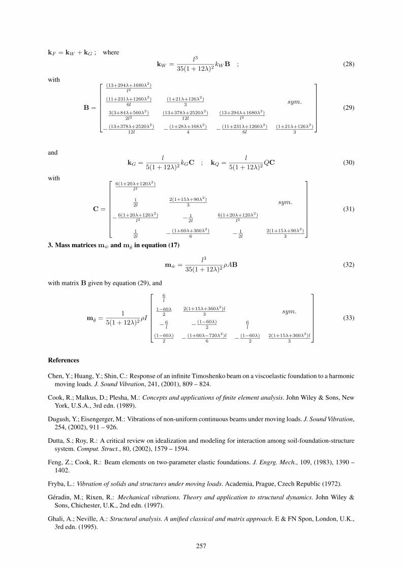
kF = kW + kG ; where
kW =l3
35(1 + 12λ)2kW B ; (28)
with
B =
(13+294λ+1680λ2)l2
(11+231λ+1260λ2)6l
(1+21λ+126λ2)3 sym.
3(3+84λ+560λ2)2l2
(13+378λ+2520λ2)12l
(13+294λ+1680λ2)l2
− (13+378λ+2520λ2)12l − (1+28λ+168λ2)
4 − (11+231λ+1260λ2)6l
(1+21λ+126λ2)3
(29)
andkG =
l
5(1 + 12λ)2kGC ; kQ =
l
5(1 + 12λ)2QC (30)
with
C =
6(1+20λ+120λ2)l2
12l
2(1+15λ+90λ2)3 sym.
− 6(1+20λ+120λ2)l2 − 1
2l6(1+20λ+120λ2)
l2
12l − (1+60λ+360λ2)
6 − 12l
2(1+15λ+90λ2)3
(31)
3. Mass matrices mw and mθ in equation (17)
mw =l3
35(1 + 12λ)2ρAB (32)
with matrix B given by equation (29), and
mθ =1
5(1 + 12λ)2ρI
6l
1−60λ2
2(1+15λ+360λ2)l3 sym.
− 6l − (1−60λ)
26l
(1−60λ)2 − (1+60λ−720λ2)l
6 − (1−60λ)2
2(1+15λ+360λ2)l3
(33)
References
Chen, Y.; Huang, Y.; Shin, C.: Response of an infinite Timoshenko beam on a viscoelastic foundation to a harmonicmoving loads. J. Sound Vibration, 241, (2001), 809 – 824.
Cook, R.; Malkus, D.; Plesha, M.: Concepts and applications of finite element analysis. John Wiley & Sons, NewYork, U.S.A., 3rd edn. (1989).
Dugush, Y.; Eisengerger, M.: Vibrations of non-uniform continuous beams under moving loads. J. Sound Vibration,254, (2002), 911 – 926.
Dutta, S.; Roy, R.: A critical review on idealization and modeling for interaction among soil-foundation-structuresystem. Comput. Struct., 80, (2002), 1579 – 1594.
Feng, Z.; Cook, R.: Beam elements on two-parameter elastic foundations. J. Engrg. Mech., 109, (1983), 1390 –1402.
Fryba, L.: Vibration of solids and structures under moving loads. Academia, Prague, Czech Republic (1972).
Geradin, M.; Rixen, R.: Mechanical vibrations. Theory and application to structural dynamics. John Wiley &Sons, Chichester, U.K., 2nd edn. (1997).
Ghali, A.; Neville, A.: Structural analysis. A unified classical and matrix approach. E & FN Spon, London, U.K.,3rd edn. (1995).
257
Hetenyi, M.: Beams on elastic foundation. The University of Michigan Press, Ann Arbor, U.S.A. (1946).
Kien, N. D.: Post-buckling behavior of beam on two-parameter elastic foundation. Int. J. Struct. Stab. Dynam., 4,(2004), 21 – 43.
Kocaturk, T.; Simsek, M.: Vibration of viscoelastic beams subjected to an eccentric compressive force and aconcentrated moving harmonic force. J. Sound Vib., 291, (2006), 302 – 322.
Luo, Y.: Explanation and elimination of shear locking and membrane locking with field consistence approach.Comput. Methods Appl. Mech. Engrg., 162, (1998), 249– 269.
Maple: Language reference manual. Spring-Verlag, New York, U.S.A. (1991).
Naidu, N.; Rao, G.: Vibrations of initially stressed uniform beams on a two-parameter elastic foundation. Comput.Struct., 57, (1995), 941 – 943.
Rao, G.: Large-amplitude free vibrations of uniform beams on Pasternak foundation. J. Sound Vib., 263, (2003),954 – 960.
Shames, I.; Dym, C.: Energy and finite element methods in structural mechanics. McGraw-Hill, New York, U.S.A.(1985).
Thambiratnam, D.; Zhuge, Y.: Free vibration analysis of beams on elastic foundation. Comput. Struct., 60, (1996),971 – 980.
Timoshenko, S.; Young, D.; Weaver, W.: Vibration problems in engineering. John Wiley, New York, U.S.A., 4thedn. (1974).
Yokoyama, T.: Vibration analysis of Timoshenko beam-column on two-parameter elastic foundation. Comput.Struct., 61, (1996), 995 – 1007.
Address: Dr. Nguyen Dinh Kien, Institute of Mechanics, Vietnam Academy of Science and Technology, 224 DoiCan Street, Hanoi, Vietnam.email: [email protected]