DYNAMIC SIMULATION OF BLIND CONTROL STRATEGIES FOR VISUAL COMFORT AND ENERGY BALANCE ANALYSIS Jan Wienold 1 1 Fraunhofer Institute for Solar Energy Systems, Heidenhofstr. 2, D-79110 Freiburg, Germany Email: [email protected]ABSTRACT The presented study describes a method for evaluating control strategies for shading devices. The method is based on dynamic lighting simulations with RADIANCE and DAYSIM and explores energy, daylight supply and visual comfort parameters at the same time. In order to include the glare aspect more effectively in dynamic building simulations, a simplified glare measure “Daylight Glare Probability simplified (DGPs)” is presented and validated for situations when the sun does not hit the eye directly. For the evaluation of the solar thermal loads, a simplified method based on RADIANCE and DAYSIM is described to calculate dynamically the energy flux through facades for external mounted shading devices. The evaluation of different simulated shading control strategies show that the commonly used manual control strategies hardly activate the shading in summer. Therefore, the solar loads in summer for these strategies are very high and at the same time glare and low contrasts at the visual display unit (VDU) occur. The automated cut-off strategy seems to be a good compromise between energy and comfort aspects, especially in summer. KEYWORDS Lighting simulation, RADIANCE, glare, control algorithm, blinds INTRODUCTION In non-residential buildings, the energy demand and the comfort are significantly influenced by the facade. To protect the building from massive solar loads in the summer and to prevent glare, movable shading devices like Venetian blinds are often used in Mid-European countries. The algorithms controlling the shading devices (e.g. manual, cut-off, closing during high irradiation) greatly affect the solar radiation flux and thus the illuminance distribution, the visual and thermal comfort and last but not least the energy demand of a building. Because many existing automatic control strategies for shading devices do not lead to a higher level of visual or thermal comfort, they are often rejected by the users. Objectives This paper shows a method which can be used to investigate different control strategies for shading devices. Their impact on energy demand and visual comfort is studied. This evaluation is done in the context of building simulation programs, and therefore the control of the shading, regardless if it is manual or automatic, is described by algorithms and/or rules. Using the presented method, any controls can be evaluated, regardless if the algorithm is based on real user patterns or purely hypothetical user patterns. To determine one of the most important factors of visual comfort -- the glare aspect -- a simplified method based on the vertical eye illuminance is proposed in order to calculate dynamically the probability of glare sensation. The suggested methods may help in developing new façade controllers (algorithms) by assessing enhanced control strategies dynamically in short time steps. Additionally, this method enables the user to generate time series of solar loads which can be used as input for thermal simulation programs. SIMULATION METHOD Dynamic daylight simulations are time consuming. Especially when shading devices are simulated, the calculation time is greatly increased. Thus, it is not possible to carry out instantaneous dynamic simulations which consider a lot of different shading positions, (as needed when investigating control strategies). The idea of the presented method is based on the pre-calculation of all necessary daylighting information using the RADIANCE (Ward et al. 1998) simulation environment. RADIANCE uses a backward raytracer and is capable of simulating specular (glossy) materials. This is very important for the correct calculation of the light transport through blinds and also for glare prediction. Of course, time- series simulations are of interest for the investigation of control strategies. To generate those time series
Transcript
DYNAMIC SIMULATION OF BLIND CONTROL STRATEGIES FOR VISUAL COMFORT AND ENERGY BALANCE ANALYSIS
Jan Wienold1
1Fraunhofer Institute for Solar Energy Systems, Heidenhofstr. 2, D-79110 Freiburg, Germany Email: [email protected]
ABSTRACT The presented study describes a method for evaluating control strategies for shading devices. The method is based on dynamic lighting simulations with RADIANCE and DAYSIM and explores energy, daylight supply and visual comfort parameters at the same time.
In order to include the glare aspect more effectively in dynamic building simulations, a simplified glare measure “Daylight Glare Probability simplified (DGPs)” is presented and validated for situations when the sun does not hit the eye directly.
For the evaluation of the solar thermal loads, a simplified method based on RADIANCE and DAYSIM is described to calculate dynamically the energy flux through facades for external mounted shading devices.
The evaluation of different simulated shading control strategies show that the commonly used manual control strategies hardly activate the shading in summer. Therefore, the solar loads in summer for these strategies are very high and at the same time glare and low contrasts at the visual display unit (VDU) occur. The automated cut-off strategy seems to be a good compromise between energy and comfort aspects, especially in summer.
KEYWORDS Lighting simulation, RADIANCE, glare, control algorithm, blinds
INTRODUCTION In non-residential buildings, the energy demand and the comfort are significantly influenced by the facade. To protect the building from massive solar loads in the summer and to prevent glare, movable shading devices like Venetian blinds are often used in Mid-European countries.
The algorithms controlling the shading devices (e.g. manual, cut-off, closing during high irradiation) greatly affect the solar radiation flux and thus the illuminance distribution, the visual and thermal comfort and last but not least the energy demand of a
building. Because many existing automatic control strategies for shading devices do not lead to a higher level of visual or thermal comfort, they are often rejected by the users.
Objectives This paper shows a method which can be used to investigate different control strategies for shading devices. Their impact on energy demand and visual comfort is studied.
This evaluation is done in the context of building simulation programs, and therefore the control of the shading, regardless if it is manual or automatic, is described by algorithms and/or rules. Using the presented method, any controls can be evaluated, regardless if the algorithm is based on real user patterns or purely hypothetical user patterns.
To determine one of the most important factors of visual comfort -- the glare aspect -- a simplified method based on the vertical eye illuminance is proposed in order to calculate dynamically the probability of glare sensation.
The suggested methods may help in developing new façade controllers (algorithms) by assessing enhanced control strategies dynamically in short time steps. Additionally, this method enables the user to generate time series of solar loads which can be used as input for thermal simulation programs.
SIMULATION METHOD Dynamic daylight simulations are time consuming. Especially when shading devices are simulated, the calculation time is greatly increased. Thus, it is not possible to carry out instantaneous dynamic simulations which consider a lot of different shading positions, (as needed when investigating control strategies). The idea of the presented method is based on the pre-calculation of all necessary daylighting information using the RADIANCE (Ward et al. 1998) simulation environment. RADIANCE uses a backward raytracer and is capable of simulating specular (glossy) materials. This is very important for the correct calculation of the light transport through blinds and also for glare prediction. Of course, time-series simulations are of interest for the investigation of control strategies. To generate those time series
Proceedings: Building Simulation 2007
- 1197 -
(hourly time steps or shorter) the RADIANCE-DAYSIM tool is used. DAYSIM uses the daylight coefficient method and is described in (Reinhart et al. 2001). For a given office geometry, orientation and location, all possible shading positions are simulated for all time steps using the respective climate data. The results of this daylighting simulation are stored in a result-matrix. The following variables are simulated within this pre-calculation process:
Energetic/daylight supply:
• Horizontal illuminance at workplace • Total energy flux through façade
(possible only for external shading devices )
Control variables:
• Vertical irradiance on façade • Direct sun on the workplace or at eye level
Comfort variables:
• Daylight glare probability, DGP • Homogeneity g1 and g2 • Contrast ratio on VDU-screen • View contact to the exterior
After the pre-calculation process, the result-matrix is evaluated by applying different control strategies. The results include a time series of the shading position (e.g. for blinds: height and slat angle) and the respective calculated parameters for each investigated control strategy. These results can be used to optimize the algorithms or as input for a thermal simulation program.
MODEL SET UP Calculated illuminance levels and the resulting energy demand for the electric lighting are the usual goals of dynamic daylighting simulation tools like DAYSIM. In this work, DAYSIM is additionally used to calculate various visual comfort parameters as well as the total energy transmission for external shading devices.
Daylight glare probability DGP
The daylight glare probability is a measure for glare caused by daylight (Wienold et al. 2006). It describes the fraction of disturbed persons under a given daylight situation. It is defined as :
)1(16.0)1log(1018.91087.5 287.1,
2,25 +⋅
⋅+⋅⋅+⋅⋅= ∑−−
i iv
isisv PE
LEDGP
ω
with Ev: vertical illuminance at eye level [lux] Ls: Luminance of source [cd/m²] ωs: solid angle of source [-] P: Guth position index[-]
The calculation of the DGP is based on the evaluation of a picture, containing the full luminance distribution of a half hemisphere in viewing direction. It is implemented with a RADIANCE tool called evalglare. A major problem in applying the DGP to the dynamic daylight simulation DAYSIM lies in the calculation of the pictures. DAYSIM is originally designed to calculate illuminance or luminance values for given points only and not for making pictures. Within this study, two methods for the dynamic calculation of the DGP are investigated:
1. A method to calculate pictures with DAYSIM
2. A simplified DGP, based only on the vertical eye illuminance and validated with Method 1 above.
In a first step, a method was developed to generate pictures with DAYSIM at each time step. For a given view point, viewing direction and picture size, a list of calculation points and directions is generated. These calculation points can be used by DAYSIM for the luminance calculation. After the simulation, the resulting data are transferred into an image. For this study, pictures of the size 300x300 pixels are used, resulting in 90,000 calculation points. Such a picture is generated for each time step when daylight is available. All the pictures are evaluated by evalglare to calculate the DGP.
This process to generate the DGP at every time step is extremely time consuming and requires a lot of disk space. But, in this study this method serves as a reference case to compare and validate the simplified method. Therefore, the calculation effort plays a minor role, since its main purpose here is to validate the simplified DGP method.
Figure 1: Example of a DAYSIM generated picture, which is used as input for the glare evaluation with evalglare. In the window area one can see the sky
subdivisions of the daylight coefficient method used for this calculation.
To overcome the huge effort required to generate pictures at every time step of the simulations, a
Proceedings: Building Simulation 2007
- 1198 -
simplified method to calculate the DPG is investigated. In (Wienold et al. 2006), it was shown that the vertical illuminance at eye level shows a reasonable correlation to the glare perception. From this publication, a simplified DPG (named now DGPs) could be derived as:
)2(184.01022.6 5 +⋅⋅= −vEDGPs
This equation neglects the influence of individual glare sources. Therefore, it must be clear that the DGPs can be applied only if no direct sun or specular reflection of it hits the eye of the observer.
This assumption can be approved by evaluating all of the simulation data. For this, the data is divided into two groups. One group contains data, for the case when the direct sun hits the eye, the other contains the complementary data. Only those data where the DGP is within its definition range i.e. greater than 0.2, are evaluated For the case when direct radiation hits the observer’s eye, the correlation between DGP and vertical eye illuminance is very low (see figure 2). In the case, that no direct sun hits the observer’s eye, the correlation is very high (see figure 3).
illuminance at eye level for the simulated situations, when direct radiation hits the observer eye. The correlation is very low (r²=0.506). Therefore the
DGPs cannot be used, if direct radiation can hit the observer’s eye.
illuminance at eye level for the simulated situations, when direct radiation does not hit the observer´s eye.
The correlation is very high (r²=0.983).
Homogeneity g1 and g2
The homogeneity parameters describe the overall contrast in a room. They are defined as
)4,3(21max
minmin
EEg
EEg
mean
==
with
Emin: Minimum horizontal desk illuminance [lux] Emean: Mean horizontal desk illuminance [lux] Emax: Maximum horizontal desk illuminance [lux]
To determine g1 and g2 for this study, illuminance values on a grid of 30 points are calculated at each time step.
Contrast ratio on VDU-screen
The contrast ratio is defined as the ratio between white and black characters on the screen.
A good contrast ratio on a VDU display is important for effective office work. The contrast is reduced, if reflections on the screen occur. Therefore, the contrast ratio should be as high as possible.
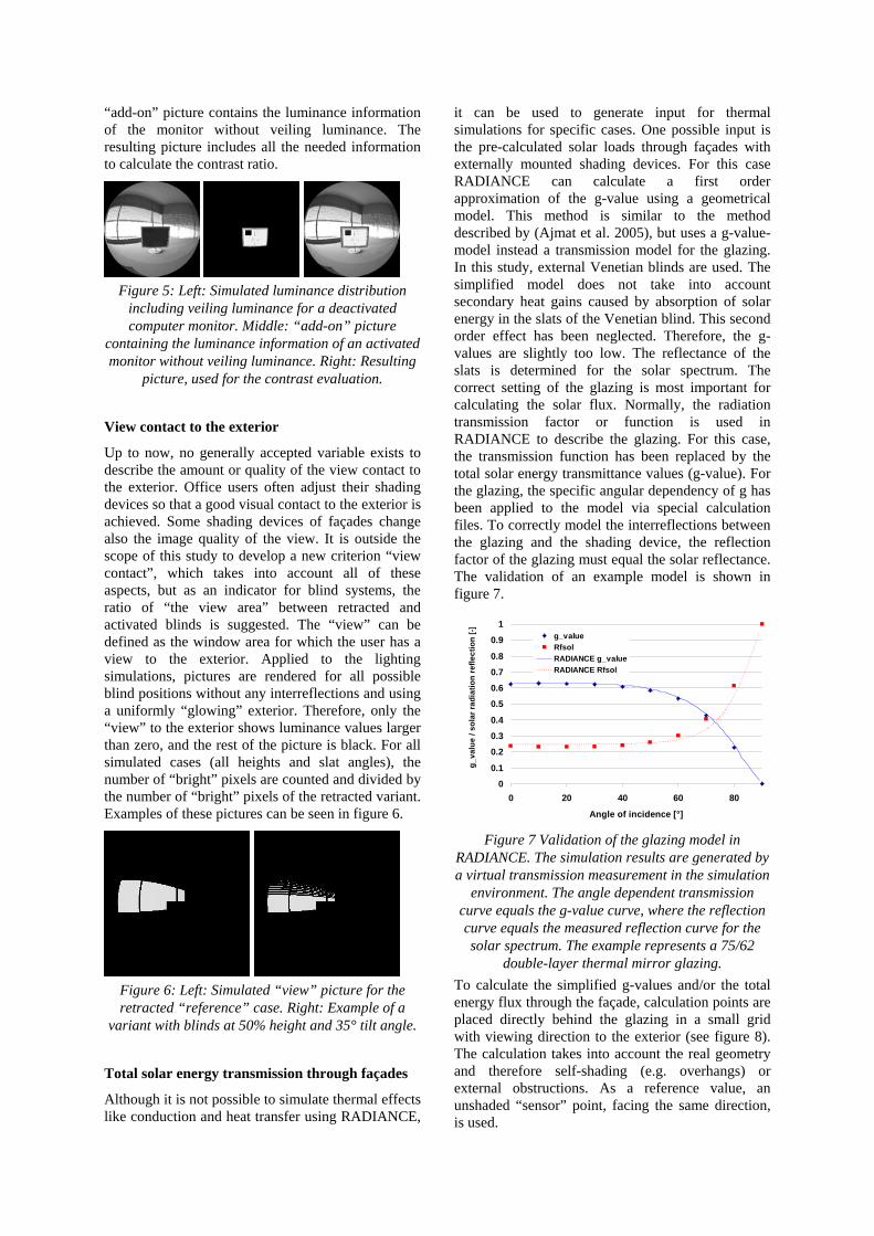
To calculate the contrast ratio, the optical behaviour of the VDU is needed. For this study, a simplified model of a TFT-flat screen monitor (Type: EIZO FlexScan L565) is used. To derive this model, measurements of the illuminance in the monitor plane and the luminance of white and black areas are taken. The comparison between this simplified model and the measurements can be seen in figure 4.
simulated luminances for white and black areas of the VDU. The simplified model takes into account the
scattering of the monitor surface being exposed to veiling illuminance.
The described model can’t be applied directly to DAYSIM, since the model itself uses self-luminant surfaces, which aren’t taken into account by DAYSIM. For the calculation with DAYSIM, the self-luminant surface is removed, so that only the veiling luminance of a deactivated monitor is calculated. To determine the resulting contrast between the white and black areas of an activated monitor, a picture is added after the simulation. This
Proceedings: Building Simulation 2007
- 1199 -
“add-on” picture contains the luminance information of the monitor without veiling luminance. The resulting picture includes all the needed information to calculate the contrast ratio.
Figure 5: Left: Simulated luminance distribution
including veiling luminance for a deactivated computer monitor. Middle: “add-on” picture
containing the luminance information of an activated monitor without veiling luminance. Right: Resulting
picture, used for the contrast evaluation.
View contact to the exterior
Up to now, no generally accepted variable exists to describe the amount or quality of the view contact to the exterior. Office users often adjust their shading devices so that a good visual contact to the exterior is achieved. Some shading devices of façades change also the image quality of the view. It is outside the scope of this study to develop a new criterion “view contact”, which takes into account all of these aspects, but as an indicator for blind systems, the ratio of “the view area” between retracted and activated blinds is suggested. The “view” can be defined as the window area for which the user has a view to the exterior. Applied to the lighting simulations, pictures are rendered for all possible blind positions without any interreflections and using a uniformly “glowing” exterior. Therefore, only the “view” to the exterior shows luminance values larger than zero, and the rest of the picture is black. For all simulated cases (all heights and slat angles), the number of “bright” pixels are counted and divided by the number of “bright” pixels of the retracted variant. Examples of these pictures can be seen in figure 6.
Figure 6: Left: Simulated “view” picture for the retracted “reference” case. Right: Example of a
variant with blinds at 50% height and 35° tilt angle.
Total solar energy transmission through façades
Although it is not possible to simulate thermal effects like conduction and heat transfer using RADIANCE,
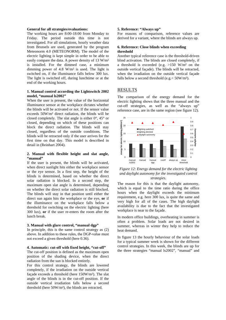
it can be used to generate input for thermal simulations for specific cases. One possible input is the pre-calculated solar loads through façades with externally mounted shading devices. For this case RADIANCE can calculate a first order approximation of the g-value using a geometrical model. This method is similar to the method described by (Ajmat et al. 2005), but uses a g-value-model instead a transmission model for the glazing. In this study, external Venetian blinds are used. The simplified model does not take into account secondary heat gains caused by absorption of solar energy in the slats of the Venetian blind. This second order effect has been neglected. Therefore, the g-values are slightly too low. The reflectance of the slats is determined for the solar spectrum. The correct setting of the glazing is most important for calculating the solar flux. Normally, the radiation transmission factor or function is used in RADIANCE to describe the glazing. For this case, the transmission function has been replaced by the total solar energy transmittance values (g-value). For the glazing, the specific angular dependency of g has been applied to the model via special calculation files. To correctly model the interreflections between the glazing and the shading device, the reflection factor of the glazing must equal the solar reflectance. The validation of an example model is shown in figure 7.
0
0.1
0.2
0.3
0.4
0.5
0.6
0.7
0.8
0.9
1
0 20 40 60 80
Angle of incidence [°]
g_valueRfsolRADIANCE g_valueRADIANCE Rfsol
g_va
lue
/ sol
ar ra
diat
ion
refle
ctio
n [-]
Figure 7 Validation of the glazing model in
RADIANCE. The simulation results are generated by a virtual transmission measurement in the simulation
environment. The angle dependent transmission curve equals the g-value curve, where the reflection curve equals the measured reflection curve for the solar spectrum. The example represents a 75/62
double-layer thermal mirror glazing. To calculate the simplified g-values and/or the total energy flux through the façade, calculation points are placed directly behind the glazing in a small grid with viewing direction to the exterior (see figure 8). The calculation takes into account the real geometry and therefore self-shading (e.g. overhangs) or external obstructions. As a reference value, an unshaded “sensor” point, facing the same direction, is used.
Proceedings: Building Simulation 2007
- 1200 -
Figure 8: Example of the placement of the
calculation points (red dots) for the g-value calculation. The grid step is here 2 cm, the distance
of the points to the façade is 1 cm. Office model example
For this study, a representative office of the following dimensions is used:
This office is a model of the test rooms at Fraunhofer ISE, which also were used for the user assessment study (Wienold et al. 2006).
The office has, in principle, two workplaces. For this study, however, only the front workplace is used (distance to façade is 1.3m for the illuminance measurement at 0.8m height, and 1.6m for the view position for the glare evaluation at 1.2 m height respectively).
Figure 9: Layout of the representative office model.
Left: Top view. Right: View towards the band façade. Shading model for the example office
For the simulation, externally mounted Venetian blinds are used. They are coloured grey (colour name:”diffuse silver”, reflection =52%) and show some glossy properties (specular reflection 5%). The simulation values are taken from spectral measurements of the blind material.
The blinds can be changed in two degrees of freedom: the height and the slat angle. For the study
all combinations of four different heights (closed by 25%,50%, 75% and 100% respectively) and fourteen different slat angles, ranging from 0° (horizontal position) to 65° (closed position) in 5° steps, are simulated. An additional variant for the retracted blinds is simulated. The geometry of all of these 57 cases and the related DAYSIM calculations are generated automatically by a script written for this purpose.
Figure 10: The blinds are simulated at four different
Figure 11: The blinds are simulated for 14 different
slat angle positions (from 0° to 65° in 5° steps): Left: 0° (horizontal), Middle: 45°, Right 65°(closed).
CALCULATION OF CONTROL STRATEGIES After the pre-calculation of the result-matrix, any control algorithm can be applied without an additional calculation effort. Therefore various strategies – regardless if they are hypothetical or realistic – can be evaluated. In this study, control strategies are discussed and compared, regardless if they are manual or automated. It is outside the scope of this work to validate or develop a manual control strategy, which describes the “real” user behaviour. Several different, hypothetical manual controls are discussed in order to evaluate their influence on the results. The application of various different control strategies can be used either to develop a real controller or to generate time series for thermal simulation programs. For this study, the following control strategies are investigated:
2.85m
3.61m
3.61m
4.61m
Proceedings: Building Simulation 2007
- 1201 -
General for all strategies/evaluations: The working hours are 8:00-18:00 from Monday to Friday. The period outside this time is not investigated. For all simulations, hourly weather data from Brussels are used, generated by the program Meteonorm 4.0 (METEONORM). The model of the electric lighting is kept simple in order to be able to easily compare the data. A power density of 13 W/m² is installed. For the dimmed case, a minimum dimming power of 4.8 W/m² is used. The light is switched on, if the illuminance falls below 300 lux. The light is switched off, during lunchtime or at the end of the working hours. 1. Manual control according the Lightswitch 2002 model, “manual ls2002” When the user is present, the value of the horizontal illuminance sensor at the workplace dictates whether the blinds will be activated or not. If the sensor value exceeds 50W/m² direct radiation, the blinds will be closed completely. The slat angle is either 0°, 45° or closed, depending on which of these positions can block the direct radiation. The blinds will stay closed, regardless of the outside conditions. The blinds will be retracted only if the user arrives for the first time on that day. This model is described in detail in (Reinhart 2004). 2. Manual with flexible height and slat angle, “manual” If the user is present, the blinds will be activated, when direct sunlight hits either the workplace sensor or the eye sensor. In a first step, the height of the blinds is determined, based on whether the direct solar radiation is blocked. In a second step, the maximum open slat angle is determined, depending on whether the direct solar radiation is still blocked. The blinds will stay in that position until either the direct sun again hits the workplace or the eye, or if the illuminance on the workplace falls below a threshold for switching on the electric lighting (here 300 lux), or if the user re-enters the room after the lunch break. 3. Manual with glare control, “manual dgp” In principle, this is the same control strategy as (2) above. In addition to these rules, the DGP-value must not exceed a given threshold (here 0.36). 4. Automatic: cut-off with fixed height, “cut-off” The cut-off position is defined as the maximum open position of the shading device, when the direct radiation from the sun is blocked entirely. For this control strategy, the blinds are lowered completely, if the irradiation on the outside vertical façade exceeds a threshold (here 150W/m²). The slat angle of the blinds is in the cut-off position. If the outside vertical irradiation falls below a second threshold (here 50W/m²), the blinds are retracted.
5. Reference: “Always up” For reasons of comparison, reference values are derived for a variant, where the blinds are always up. 6. Reference: Close blinds when exceeding threshold Another typical reference case is the threshold-driven blind activation. The blinds are closed completely, if a threshold is exceeded (e.g. >150 W/m² on the outside vertical façade). The blinds will be retracted, when the irradiation on the outside vertical façade falls below a second threshold (e.g.< 50W/m²).
RESULTS The comparison of the energy demand for the electric lighting shows that the three manual and the cut-off strategies, as well as the “always up” reference case, are in the same region (see figure 12).
Figure 12: Energy demand for the electric lighting and daylight autonomy for the investigated control
strategies. The reason for this is that the daylight autonomy, which is equal to the time ratio during the office hours when the daylight exceeds the minimum requirement, e.g. here 300 lux, is quite the same and very high for all of the cases. The high daylight availability is due to the fact that the investigated workplace is near to the façade.
In modern office buildings, overheating in summer is often a problem. Solar loads are not desired in summer, whereas in winter they help to reduce the heat demand.
In figure 13 the hourly behaviour of the solar loads for a typical summer week is shown for the different control strategies. In this week, the blinds are up for the three strategies “manual ls2002”, “manual” and
Proceedings: Building Simulation 2007
- 1202 -
“always up” and lead to high solar loads.
0
10
20
30
40
50
60
70
80
90
100
time (summer week)
spec
ific
sola
r loa
d [W
/m²fl
oor a
rea]
manual ls2002 manualmanual dgp cutoffalways up close threshold
Figure 13: Specific solar loads (related to the floor area) in an exemplary summer week for the different
control strategies. The reason for this is that the sun position in summer is very high, and therefore the direct sun does not enter very deeply into the room. Therefore, the trigger for activating the blinds (e.g. 50W/m² direct radiation at the workplace) is not set and the blinds stay retracted. This behaviour leads to much higher solar loads for “manual ls2002” and “manual dgp” compared to the “cut-off” strategy. For example for the peak loads, the “manual ls2002” is greater by a factor of 2.5 and the “manual dgp” by a factor of 1.7 compared to the “cut-off” strategy.
The effective g-value (Kuhn 2006) is the total sum of the solar load passing the façade divided by the total sum of the solar irradiation hitting the façade on the outside. It takes into account direct and diffuse irradiation. This value is an indicator, how much solar energy is passing through the façade in a specified period. The comparison of the effective g-values for summer and winter shows that the cut-off strategy leads throughout the year to significantly lower values compared to all the manual strategies (See figure 14).
0
0.1
0.2
0.3
0.4
0.5
0.6
manualls2002
manual manual dgp cutoff always up closethreshold
effe
ctiv
e g-
valu
e
wintersummer
Figure 14: Effective g-values for the summer ( May 1
– Sep. 30) and the winter ( Oct. 1 – April 30) periods.
In the following figure, the cumulated DGP is shown for the different control strategies. In a previous study (Wienold 2007) it was determined that the user adjusted the blinds, so that a DGP of 0.36 resulted. For the “manual ls2002” and “manual” control strategy, this threshold value is exceeded in about
1100 h of office time. Further, the DGP exceeded 0.5, which is rather high, for about 400h in these two strategies. For the cut-off strategy, a value of 0.5 was exceeded only at16h. Of course, the glare optimized strategy “manual dpg” meets very well the DGP of 0.36.
different control strategies. Only office hours are taken into account.
Upon the investigation of the cumulated view ratio. it reveals again that the blinds are very frequently retracted (in about 2000h of office time) for the “manual ls2002” and the “manual” strategies. If we assume a reasonable view for a view ratio larger than 0.4, the cut-off strategy meets that value in about 2000h of office time. This value must be confirmed by future user assessment tests, which are foreseen at Fraunhofer ISE in 2007 and 2008.
0
0.2
0.4
0.6
0.8
1
0 500 1000 1500 2000 2500office hourcs [h]
view
ratio
[-] manual ls2002
manualmanual dgpcutoffalways upclose threshold
Figure 16: Cumulated hours of the view ratio for the
different control strategies. Only office hours are taken into account. The view ratio describes the
“amount” of view to the exterior.
During the main office hours, a value larger than 5 is aspired to for the contrast ratio on a VDU screen The “cut off” and “manual dgp” fall below this value for less than 10 hours per year, whereas the “manual ls2002” falls below this value for about 550h per year. (See also figure 17.)