National Aeronautics and Space Administration Scientific and Technical Information Division 1989 NASA Technical Memorandum 4083 Analysis of an Unswept Propfan Blade With a Semiempirical Dynamic Stall Model T. S. R. Reddy Tbe University of ToZedo ToZedo, Ohio K. R. V. Kaza Lewis Research Center CZeveZand, Ohio https://ntrs.nasa.gov/search.jsp?R=19890005741 2020-01-15T18:30:32+00:00Z
Transcript
National Aeronautics and Space Administration
Scientific and Technical Information Division
1989
NASA Technical Memorandum 4083
Analysis of an Unswept Propfan Blade With a Semiempirical Dynamic Stall Model
T. S. R. Reddy Tbe University of ToZedo ToZedo, Ohio
K. R. V. Kaza Lewis Research Center CZeveZand, Ohio
Summary The time-history response of a propfan wind-tunnel model
with dynamic stall was studied analytically. The response obtained from the analysis was compared with available experimental data. The governing equations of motion were formulated in terms of blade normal modes calculated using the COSMIC-NASTRAN computer code. The response analysis considered the blade plunging and pitching motions. The lift, drag, and moment coefficients for angles of attack below the static stall angle were obtained from a quasi-steady theory. For angles above static stall angles, a semiempirical dynamic stall model based on a correction to the angle of attack was used to obtain lift, drag, and moment coefficients. Using these coefficients, the aerodynamic forces were calculated at a selected number of strips, and integrated to obtain the total generalized forces. The combined momentum-blade element theory was used to calculate the induced velocity.
The semiempirical stall model predicted a limit cycle oscillation near the setting angle at which large vibratory stresses were observed in an experiment. The predicted mode and frequency of oscillation also agreed with those measured in the experiment near this setting angle. The results also correlated well with the other published data that used a semiempirical dynamic stall model based on a synthesized procedure.
Introduction Modern propeller designs are being considered to power
transport aircraft at high subsonic speeds. These new propeller designs, called propfans, are expected to result in significant savings in fuel consumption. Figure 1 shows the characteristics of a typical propfan. Compared to a conventional propeller, the number of blades and width of the blade chord of the
Figure 1 .-Wind tunnel model of a
propfan are increased to provide a high disk loading. The blades are thin to increase the drag divergence Mach number and are swept to reduce the local effective Mach number and noise. Flutter analysis of these propfans is needed to determine the critical (flutter) speed below which the aircraft has to operate to avoid catastrophic blade failure. A response analysis is needed to determine the stresses and fatigue life of the blades. The aeroelastic response and flutter analyses of prop- fans are ongoing research efforts at NASA Lewis Research Center. Flutter analysis methods and experimental flutter results for propfans at low angles of attack (classical flutter) are described in references 1 to 4. The analyses include the effects of number of blades (cascade effects), blade pitch angle, blade sweep, and mistuning.
However, under static or low-speed conditions, the propfan sections may operate at high angles of attack and have the potential to stall flutter, which is triggered by separated flow during part of every cycle of oscillation. Stall-flutter speeds are very low compared to classical flutter speeds, and the resulting vibratory stresses can cause fatigue failure of the propfan. Hence, avoiding stall flutter is a critical design condi- tion, and analysis of stall flutter and prediction of unsteady forces due to flow separation are critical research needs.
In steady flow, above a certain critical angle of attack, the flow over an airfoil breaks down-a phenomenon called static stall (flow separation). In the case of an oscillating airfoil this stall phenomenon is referred to as dynamic stall. There has been considerable research to understand dynamic stall and its effects (refs. 5 and 6) . The three important effects of dynamic stall are shown schematically in figure 2, and are summarized as follows:
(1) Stall delay-An airfoil with a positive rate of angle of attack (upstroke) stalls at an angle of attack greater than the
STALL DELAY
_ _ _ _
-- / ‘-STATIC DATA
/ /
/
ANGLE OF ATTACK,U
Figure 2.-Three unsteady effects of dynamic stall. propfan.
1
static stall angle. This means that an oscillating airfoil can reach higher angles of attack than a static airfoil can reach before the tlow separates. The stall recovery (reattachment) during a negative rate of angle of attack (downstroke) generally occurs at an angle less than the static stall angle.
(2) Overshoot of the forces and moments-The vibratory forces and moments are considerably higher than those for the static counterparts. This affects stresses and the fatigue life of the propfan.
(3) Negative aerodynamic damping-The dynamic stall events-namely, scparation o f the flow, formation of the vortex. movement of the vortex, and reattachment-take a finite time to develop. However, once the flow is separated, the dynamic stall events introduce two important physical consequences. The first is the hysteresis produced by the lag and asymmetry of the airloads with respect to the motion o f the body. This is in contrast to the quasi-steady case where no hysteresis is produced since the flow field adjusts immediately t o each change in angle of attack. The second consequence is aerodynamic damping. which is related to the net work done ovcr a complete cycle of oscillation. If this damping is negative, the airfoil extracts energy from the airstream. This is the condition of flutter. Stall flutter, arising from this negative damping. tends to occur when the airfoil is oscillating in and out of stall.
Attempts to predict these effects due to dynamic stall fol- low two approaches, one theoretical, and the other based on experimental data (semiempirical) (refs. 5 to 7). The theoretical approaches attempt to solve the fluid mechanics equations in their fundamental form by numerical techniques with varying degrees of simplifications and assumptions. These include evaluating the flow field using the Navier-Stokes equations, the discrete vortex methods, and the coupled viscous-inviscid methods (zonal methods). These methods, in addition to their limited development. require significant computer time and therefore are not suitable for routine aeroelastic analysis.
The semiempirical models attempt to simulate the gross features of stall. The various parameters in these models are determined by fitting theory to experimental data obtained from oscillating airfoil tests. These models gained much interest for the following reasons: ( I ) They use static airfoil data (lift, drag, and moment coefficients for different angles of attack at different Mach numbers) with a correction for dynamic (unsteady) effects. This is advantageous because static airfoil data can be easily generated and automatically include the effects of Reynolds number, Mach number. and airfoil shape; and ( 2 ) the models take less computer time, so they can be used in a routine aeroelastic analysis.
The empirical parameters used in these semicmpirical nioclels are usually based on the experimental data obtained from airfoils oscillating in pitch about quarter chord. However, an arbitrary motion includes both pitch and plunge motions. So stall modeling should include separate plunge motion terms in the identification of the empirical parameters. Many of the
existing semiempirical models do not take into account the distinction between pitch and plunge motions. In order to use the existing empirical models in an aeroelastic analysis where the unsteady motion consists of both plunging and pitching, an equivalent angle of attack based on both the pitch and plunge motions of the airfoil is calculated and used.
The objective of the present effort is to predict the stall- flutter behavior of a propfan wind-tunnel model using a scmienlpirical dynamic stall model. Wind-tunnel experiments o f the SR-2 propfan (SR for single rotation and 2 for design number 2) have indicated that it is prone to stall flutter at static thrust (zero wind speed) conditions (refs. 8 and 9). The buildup of high stresses at noncritical speeds during the experiment is taken as the condition indicating stall flutter. The experi- ments showed that the stall flutter response occurred in the third mode (first torsion). In reference 5 . three semiempirical dynamic stall models are compared with respect to lift, drag, and moment coefficients by applying them to airfoils oscillating sinusoidally. The three models are the Gormont model (ref. I O ) , the Gangwani model (ref. 1 I ) . and the ONERA model (ref. 12). These are referred to in reference 5 as models A. B. and C , respectively. Of these models. the Gormont model requires only o n e empirical stall paramctcr, which is given as a function of Mach number and airfoil thickness to chord ratio. The Gangwani and ONERA models require a large number of dynamic stall parameters that depend on the airfoil section used. These parameters are not available for propfan airfoil sections (NACA 16 series). Therefore. in the present study, the Gormont model is used t o analyze the SR-2 propfan wind-tunnel model.
Reference 8 presents analytical stall-flutter results for the SR-2 propfan based on a linear structural model and a linear aerodynamic model which are based on the theory presented in reference 13. The results predict the mode and the blade setting angle for which stall flutter occurred in tests. However, this analysis is insufficient since the present problem is nonlinear both structurally (because of large deflections) and aerodynamically (because of high angle of attack and separated flow). The analysis of reference 8 only predicts the onset of stall flutter; it does not calculate the limit amplitude response of the propfan blade. An analytical model of the SR-2 propfan for stall flutter also is presented in reference 14. This analysis uses a nonlinear beam structural model and the Gangwani dynamic stall model (model B). The dynamic stall data of an NLR-1 airfoil (ref. 1 1 ) are used since dynamic stall data for the NACA 16 series are not available. The analysis qualitatively predicts the stall-flutter behavior of the SR-2 propfan blade at static thrust conditions.
The present analysis differs from that of references 8 and 14 in that a nonlinear, large-deflection finite element formu- lation is used in modeling the structural behavior of the propfan. This formulation results in more accurate repre- sentation of the deformed steady and modal blade geometry than is obtained with a beam formulation. The present formulation is also more suitable for application to other swept
propfans made of composite materials. The model-A dynamic stall model, where Mach number and thickness effects are accounted for in the stall model, is used for aerodynamic calculations. This simulates the approximate dynamic stall effects of NACA 16 series airfoils, rather than the NLR-I airfoil dynamic stall effects used in reference 14. In contrast to the linear structural and aerodynamic model of reference 8, the present model includes nonlinear structural and aero- dynamic forces and dynamic stall effects. The numerical study is performed for a single blade by neglecting structural and aerodynamic coupling between blades. The results are compared with the theoretical results of reference 14 and with experimental data of reference 8.
In the following sections, first the governing equations of motion are given, and then the results and discussion of a numerical stall-flutter study with the computer code developed are presented. As an aid to the reader, a symbols list is given in appendix A.
I
Aeroelastic Equations of Motion Coordinate Systems
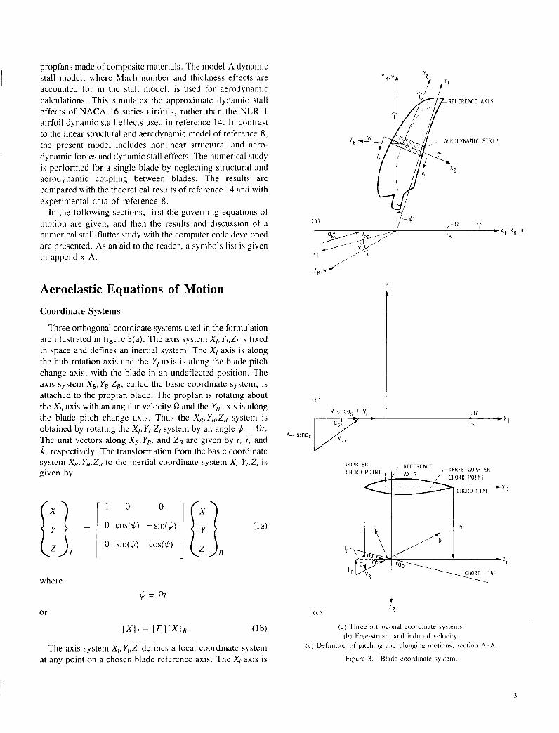
Three orthogonal coordinate systems used in the formulation are illustrated in figure 3(a). The axis system X,, Y,,Z, is fixed in space and defines an inertial system. The X , axis is along the hub rotation axis and the Y, axis is along the blade pitch change axis, with the blade in an undeflected position. The axis system X,, YB,ZB, called the basic coordinate system, is attached to the propfan blade. The propfan is rotating about the X , axis with an angular velocity R and the YE axis is along the blade pitch change axis. Thus the XB,YB,ZB system is obtained by rotating the X,, Y,,Z, system by an angle $ = Rr. The unit vectors along X,,Y,, and Z, are given by ;, j , and I, respectively. The transformation from the basic coordinate system Xn, Yn.Zn to the inertial coordinate system X,, Y,.Z, is given by
where * = Rt
or
( X I / = [ T l l { x l B (1b)
The axis system X,, Yt,Zt defines a local coordinate system at any point on a chosen blade reference axis. The X t axis is
y n ' v T A X I S
S l R l P
OllARTFR ITHRFE-QUARTFR
CIIORII POINT
CllQRD L I N E 'f
(a) 'I'hree or thogmal coordinate systems. (b) Free-stremi and induced velocity
( c ) Definition of pitching and plunging motions. section A-A
Figure 3.-Blade coordinate system
3
normal to the reference axis and is positive from leading edge to trailing edge; the Y,' axis is along the tangent to the reference axis at the point under consideration and is positive in the direction of propfan root to tip; and the Zt axis is perpendicular to both X!, and Y,, and is positive in the direction of a right-handed system. The unit vectors along X,,v. , and Z,. are given respectively by t , f, and i l . The relation between the basic coordinate system and local coordinate system can be written as
where [ T2] , the transformation matrix, can be calculated from the geometry of the propfan blade. A brief explanation of the calculation procedure is given in appendix B. It should be noted that the transformation matrix [Tz] varies from point to point on the reference axis. In general, the blade deforms to a steady- state position about which the perturbation (vibratory) motion is superimposed. In the present analysis the steady displace- ments are assumed to be caused by the centrifugal forces only. The local coordinate system and the transformation matrix, [Tz] , are calculated with reference to the steady-state position of the blade. This nieans that the aeroelastic analysis presented in this report is, in fact, a quasi-linear analysis, where a linearized structural model is coupled with a nonlinear aerodynamic model.
Equations of Motion
The governing equations of motion for the propfan are formulated in terms of normal modes. The blade is considered to be fixed at one end and free at the other. The normal modes of the rotating propfan can be obtained from a finite element analysis program that includes a geometric nonlinear analysis to account for the large deflections and rotational effects of the propfan. The finite element analysis results in a large number of nonlinear governing equations of motion that are computationally expensive to solve. However, the govern- ing equations of motion can be linearized, which permits simplification of the equations; they can be expressed as a superposition of normal modes, which reduces the large number of equations. The formation, linearization, and conversion of the governing equations of motion into equations in normal coordinates for a propfan are described in reference 3. In the present report only the calculation of generalized aerodynamic forces is presented. The final governing equations of motion for each mode can be written as
where in, is the ith generalized mass, w , is the circular frequency in the ith normal mode, 5; is the critical damping (structural) ratio in the ith mode, Q, is the ith generalized force including aerodynamic contributions, NM is the number
of normal modes used in the analysis, and q, is the ith normal coordinate. which is a function of time.
Generalized Aerodynamic Forces
In the present study. strip theory is used to calculate the generalized aerodynamic forces on the blade. The blade is divided into a series of discrete aerodynamic strips that are normal to an arbitrary reference line (reference axis). One of these strips is shown in figure 3(a). Each strip has two motions: ( I ) plunging and (2) pitching about the arbitrary reference line. The generalized forces calculated at each strip along the radius of the blade are integrated to obtain the total generalized force (a,) in each mode. The two-dimensional, incompressible. quasi-steady theory is used in calculating the velocities and forces. Stall effects are included via a semiempirical dynamic stall model. The noncirculatory lift and moment associated with apparent mass forces are neglectcd. The classical combined momentum-blade element theory, as given in appendix C, is used to calculate the steady induced velocity. It is also assumed that the spanwise velocity component (along the Y,. axis) does not contribute to the aerodynamic loads.
With the above assumptions. the calculation of the aerodynamic part of Q, involves the calculation of ( I ) the relative velocity at a point on the reference line of the airfoil and the angle of attack, (2) the unsteady force coefficients, and (3) the generalized aerodynamic forces. These calculations follow.
(1) Relative velocity a n d angle of attack calculation.-To calculate the aerodynamic loads, one must calculate the velocity of a point on the reference axis of the blade relative to the air velocity. This velocity is calculated in the blade local coordinate system. The contributions to the relative velocity are (a) oncoming wind and induced velocity and (b) velocity due to blade rotation and vibratory motion.
(a) Wind velocity and induced velocity (fig. 3(b)): The oncoming air makes an angle, cy,,, with respect to the normal of the disk plane. Therefore the components in the X, direc- tion and in the plane of the disk are V, cosa, and V, sina,. Let the steady induced velocity be given by V,, which acts in the positive direction of X,. Then, ( V ) u , the velocity contribution from airflow in the local coordinate system (fig. 3(b)), is given by
I V I , =
v, coscy, + VI
V, sina,
0
(4)
(b) Velocity contribution from blade motion and rotation: The propfan is rotating about the X, axis. Let uo, V g , and wo be the steady displacements due to centrifugal loads, and u , v, and IC be the unsteady (perturbed) displacements due to
4
Appendix D Effect of Airfoil Static Data Variation on the Dynamic Stall Response
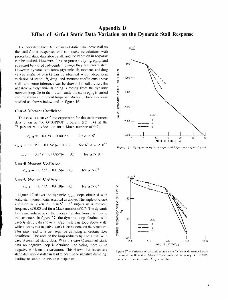
To understand the effect of airfoil static data above stall on the stall-flutter response, one can make calculations with prescribed static data above stall, and the variation in response can be studied. However, for a response study, cp, c, '4 cd cannot be varied independently since they are interrr However, dynamic stall loops (dynamic lift, moment, and drag versus angle of attack) can be obtained with independent variation of static lift, drag, and moment coefficients above stall, and some inference can be drawn. In stall flutter, the negative aerodynamic damping is mostly from the dynamic moment loop. So in the present study the static c, , /~ is varied and the dynamic moment loops are studied. Three cases are studied as shown below and in figure 16.
Case-A Moment Coefficient
This case is a curve-fitted expression for the static moment data given in the G400PROP program (ref. 14) at the 75-percent-radius location for a Mach number of 0 .7 ,
~,,,/4 = -0.035 - 0.003*a for a < 6"
= -0.053 - O.O24*(a - 6.0) for 6" < a < 10"
= -0.149 - O.O085*(a - 10) for ct > 10"
Case-B Moment Coefficient
cmCl4 = -0.553 - 0.015(a - 6) for a > 6"
Case-C Moment Coefficient
c , , , , ~ ~ = -0.553 - O.OlO(ct - 6) for ct > 6"
Figure 17 shows the dynamic c, , /~ loops obtained with static-stall moment data assumed as above. The angle-of-attack variation is given by a = 5" + 3" sin(wt) at a reduced frequency of 0.05 and for a Mach number of 0.7. The dynamic loops are indicative of the energy transfer from the flow to the structure. In figure 17, the dynamic loop obtained with case-A static data shows a large hysteresis loop above stall, which means that negative work is being done on the structure. This may lead to a net negative damping at certain flow conditions. The area of the loop reduces by about half with case-B assumed static data. With the case-C assumed static data no negative loop is obtained, indicating there is no negative work on the structure. This shows that inaccv,.ate static data above stall can lead to positive or negative damping, leading to stable or unstable response.
0x104 r + L
w u LL LL W 0 U
c z z u z 5 0 CL W 4
> n 5 c v)
ANGLE OF ATTACK, a
Figure 16.-Variation of static moment coefficient with angle of attack.
100' 2.0 4.0 6.0 8.0 10.0
ANGLE OF ATTACK, a
Figure 17.-Variation of dynamic moment coefficient with assumed static moment coefficient at Mach 0.7 and reduced frequency, k , of 0.05; (Y = 5 + 3 sin ks; model A dynamic stall.
19
vibration of any point on the reference axis, in the X,, Y,, and Z, directions, respectively; ug, \~ll. and \ino are functions of x, y , and z , and u , v, and u’ are functions o f x , J, z , and r , where .r, J, and : are coordinates of the point in the basic (rotating) coordinate system X,, Y,,Z,. Then the absolute velocity dddr of a point X,J,Z is given by
dF . - = r + 5 x r dt
where 0 is the angular velocity of the XB,YB,ZB coordinate system and is given by
W= Ri (6) is the rotational speed in rad/scc, and F, the position where
vector of the point under consideration, is given by
* A
F = (x + ug)i + (y + t i l j ) j + ( z + y , ) k + ui + t j + w i
= I; + ui + v j + nk (7)
where 6 represents the position vector of the point under con- sideration including steady displacements due to centrifugal loads.
The transformation ofdddr , that is, the velocity of the point .r,y,:, into the local coordinate system, is given by
where subscripts h, in, and rot indicate blade. from-blade vibratory motion, and from-blade rotation (a). respectively. In the present analysis, the components of [ VI,, are calcu- lated for points on the reference axis (reference line).
Then the relative velocity of any point on the reference axis is given by (eqs. (4) to (8))
where
The components of [ V ) are contributions from the blade motion to the velocities in the local coordinate system and are calculated as follows. First, for each strip, the modal deflections are transformed into plunge h, and pitch CY,
motions about the reference axis in the X,, Y,,Z, system. The plunge and pitch motions are shown in figure 3(c), with plunging motion being positive in the negative Z,, direction, and pitching motion being positive for the leading-edge-up (nose-up) position. Reference 3 describes the procedure of obtaining h, and cy, (for each mode) from the general vibratory motion. Then the total plunging displacement h of a point on the reference axis and the pitching displacement 01,) about the reference axis, for each strip, can be expressed as sum of the contributions from various normal modes:
IVM h = h,q,
I = I
N M
a p = “14, i = I
where hl and CY, are the contributions to total plunge and pitch motions, respectively. from the ith modal deflections, and NM is number of normal modes. Then, neglecting all other components, the velocity due to blade motion of a point on the reference axis is given by
VJ,,, =
and the rotation of the strip is given by cy!,.
The velocity vector ( VJre l (eq. (9)) can be written in terms of U(., U,, and U,i-the chordwise, tangential (spanwise), and normal components of velocity of the airfoil-as shown in figure 3(c):
The next step is to calculate the angle of attack of the strip in terms of U , , U,, and U,,. But, it is well known that the lift of the airfoil is proportional to the downwash velocity of the three-quarter chord point on the airfoil. Since U,, is the velocity perpendicular to the chord at the reference point, the sectional angle of attack can be written as
5
Fxt, = -L sin($) + D cos($)
F.,, = - L cos($) - D sin($)
Mref = M,, + La
)
where Mref refers to the moment about the reference axis and u is the distance between the reference axis and the quarter chord (positive for reference axis aft of quarter chord). Then the generalized force at the jth strip is given by
NO NO
where dl, is the width of the strip, h,(yj) and a,(?;) are the values of h, and a, in the ith mode at in the local coordinate system, and Fzt and M,,, are the force and moment calculated at this strip. The contribution from Fxi, to equation (21) is zero since the strip is assumed rigid in the chordwise direction.
Summarizing, the total generalized force from the aero- dynamic contribution in each normal mode is calculated as follows: First, the chordwise and normal velocities at any time step are calculated using equation (13). Second, the angle of attack is calculated using equation (14). If the angle of attack is above the section airfoil static stall angle, the lift, drag, and moment coefficients are calculated according to dynamic stall model A. Otherwise, they are obtained from the static airfoil tabular data for this angle of attack. Third, the generalized force on each strip is calculated using equation (21). Finally, the total generalized force on the blade for the ith mode is given by
N S Ql = A, i = 1,2, ..., NM ( 2 2 )
I = I
where NS is the number of strips (segments) the blade is divided into. This gives the system of equations (eq. 3) for this time step.
Since the governing equations of motion (eq. (3)) are nonlinear in aerodynamics, it is convenient to solve these equations in the time domain. In the present analysis the Wilson-@ method (ref. 18) is used. This method assumes a linear variation of acceleration between two time steps. The method is an implicit integration method and is unconditionally stable.
The stall response calculation procedure consists of the following steps and is shown schematically in figure 4.
( 1 ) For a given rpm and setting angle. perform a nonlinear finite element analysis, taking into account the geometric stiffness effects due to large deflections. This analysis cal- culates the steady-state deflections, free-vibration mode shapes, and natural frequencies. For example, a COSMIC-NASTRAN finite element analysis consists of two runs: (a) a NASTRAN
R f A D BI ADE GEOMEIRY
t
t
t
t
RFAD RPM I ROTATE TO D F S I R t D S E T T I N G ANGLE A 1 75 PERCFNT SPAN
PFRFORM NASIRAN GEOMETRIC NONLINEAR A N A L Y S I S . O l i l A l N NATURAL FRIQUF N C l E S ANI) MODI SHAPES
C N C U L A T E MODAL VALULS. S I E A D Y DISPLACEMENIS, TKANSFORMATION M A l R l C t S AI SELECTEI) BLADE STATIONS
READ MACH NUMBER AND C A L C U L A l t I N I I I I C F D V E L O C I T Y AT THESE STATIONS
1 I I ~~
STAR1 I IME LOOP
t i
I A T LACH SEI ECTED B L A D I S l A T I O N 1 1 k I I
- C A L C U L A I t ANGLE Or ATTACK -TEST FOR S T A T I C S l A L l -USE S T A T I C FORCE IIATA BELOW S l A l L - INCLUDE DYNAMIC SIAl I EFFECTS FOR ABOVE S T A L L -CALCUIATE G E N E R A L l l F D FORCES
I /
t CALCULATE TOTAL G I N I R A L 1 7 E D FORCE AND RtSPONSE
A 1
7 R P M RANGE COVERED?
STOP
Figure 4.-Flow chart o f aeroela\tic stall tlutter analy\is
solution-4 run to calculate and store the geometric stiffness matrix and steady-state displacements and (b) a NASTRAN solution-9 run using the geometric stiffness matrix generated previously for the frequencies and mode shapes.
(2) Enter the data obtained from step 1 into the ASTROP2 program (ref. 3) to obtain the modal values h, and a, and the transformation matrix Tz relating the basic coordinate system to the local coordinate system at selected radial stations along the blade span. However, for straight blades, using the ASTROP2 program is not necessary since the transformation matrix is a straight-forward, two-dimensional transformation.
(3) Calculate the steady. induced velocity (V , ) . In the present study, the combined momentum-blade element theory described in appendix C is used to calculate the induced
7
velocity. Specifically, the thrust calculated from momentum theory at each radial station is set equal to the thrust produced from the blade airfoil section properties. This procedure gives a nonuniform induced velocity distribution over the disk.
(4) At each strip (segment), calculate the velocity compo- nents on the strip, the angle of attack, and the generalized aerodynamic forces (eq. (21)). and obtain the total generalized force (eq. (22)).
( 5 ) Formulate the aeroelastic equations (eq. ( 3 ) ) , and run the stall-flutter code for a response calculation.
(6) For another setting angle or rpm, go back to step I .
Blade Model and Analysis Description The SR-2 model propfan has been chosen to demonstrate
the capability of the code developed with dynamic stall. Stall- flutter tests have been done for this propfan at zero and low forward speeds (refs. 8 and 9).
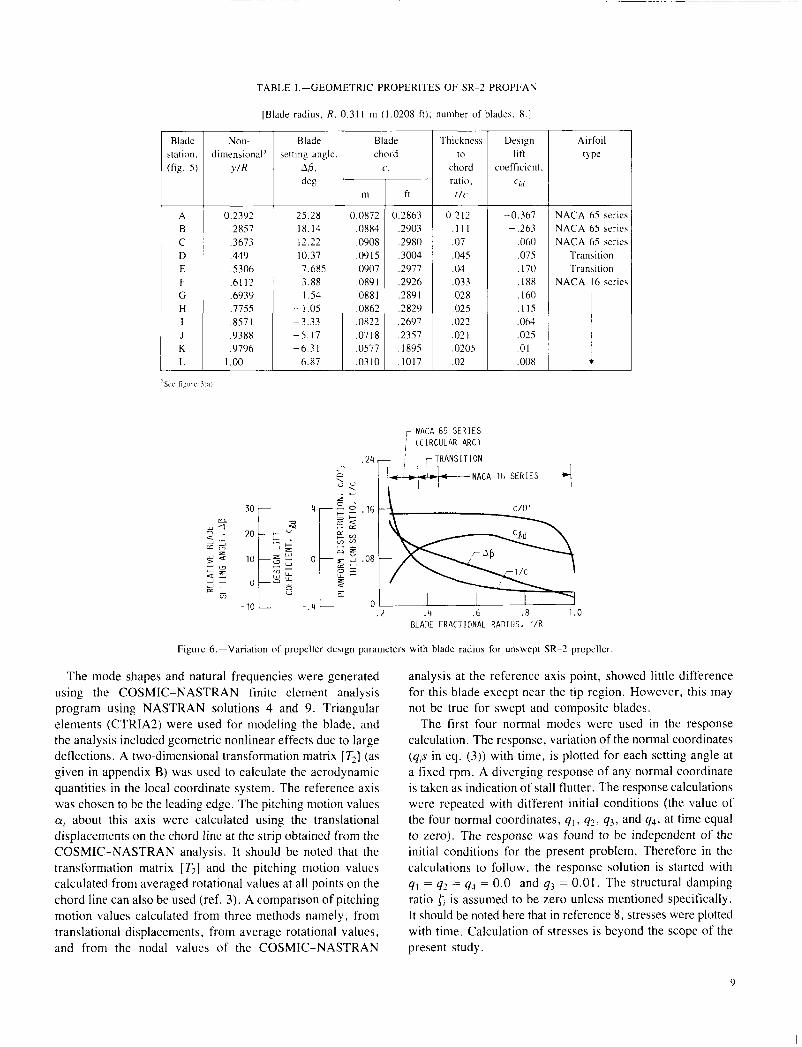
The SR-2 propfan model (ref. 19) is designed for an operating condition of Mach 0 . 8 at a 10.668-km (35 000-ft) altitude, a 243.8-mis (800-ftisec) tip speed, and a power loading of 301 kW/m' (37.5 shp/ft'). The model has cight steel blades and is 0.6233 m (2.0416 ft) in diameter D ' . The NACA 16 series airfoils are used from the tip to the 45-percent-radius portion of the blade; NACA 65 series airfoils with circular arc (CA) camber lines are used from the 37-percent radius to the root with a transition fairing con- necting the two regions. The planform of this model is shown in figure 5 . A summary of the pertinent geometric parameters is given in table I and is shown schematically in figure 6. The table shows the distribution of blade geometric twist relative to the geometric twist at 75-percent span AB, and shows chord c / D ' , thickness to chord ratio t l c , design lift coefficient c ' ~ . and airfoil type at 12 stations along the span. In addition, the blade Mach number and angle of attack a will be different at each station depending on the rotational speed. free-stream velocity, and the setting angle.
It can be inferred from the preceding paragraph that for the response calculation one needs a large amount of airfoil data- lift e[', drag cd, and moment coefficients c , , , ,~ , both in static and dynamic conditions, at several Mach numbers and angles of attack. Reference 14 uses static airfoil data (c?, cd. and c',,~~.;~) for the SR-2 blade stall-flutter analysis. These static airfoil data are for an isolated blade with no correction for cascade effects. The data are given at five spanwise stations for different Mach numbers and angles of attack; they are interpolated for other stations. However, the accuracy of the static data is not discussed in reference 14. In view of this, to assess the sensitivity of flutter speed for variations in airfoil static data above stall, a parametric investigation was con- ducted. The results from this investigation are discussed in appendix D.
In the present study, the isolated airfoil static data presented in reference 14 are used since no other static airfoil data are
BLADt STATION
L K J
1
H
G
F
E
D
C
B
A
4 .27 C M
(1.68 IN.) ROTATION A X I S $
Figure S.-Planforrn of SR-2 modcl propfan hladc
available at this time. The dynamic stall model A is used to calculate response in dynamic conditions. Structural and aero- dynamic couplings between blades (i.e, cascade effects) are disregarded. Therefore, a single propfan blade analysis is performed. The material propcrties used are a Young modulus equal to 30X lo6 psi (206.85 GN/m'), a Poisson ratio equal to 0.3, and a material density equal to 0.732X 10-j Ib-sec'/in4 ( 7 . 8 2 3 ~ lo3 kgim3).
The experimental data of reference 8 present the variation of total vibratory stress with rpm and indicate that a high stress level, excluding stress levels corresponding to rpm at critical speeds, is an indication of stall flutter or buffeting. (Ref. 8 mentions that buffeting is said to have occurred for blade setting angles above 45", that buffeting is a multiple mode excitation, and that blade motion has little effect on the load- ing.) An examination of the data presented in reference 8, indicates that the highest stress levels (taken as indicative of stall flutter) were recorded at about 8500 rpm with a blade setting angle around 30". This condition is taken as a stall- flutter condition. Therefore for the results presented here most calculations are made for 8500 rpm. However, two more cases, 2000 rpm at a 30" setting angle and 5000 rpm at a 50.3" setting angle. are also analyzed for further validation of the analysis and code. The shaft angle of attack a, (propeller t i l t angle) is taken as zero.
8
TABLE I --GEOMETRIC PROPERITES O F SR-2 PROPFAN
[Bldde radiu\. R. 0 31 I m ( 1 0208 f t ) . number of bldde\, 8 ]
.7 . 4 . 6 .8 1 . o BLADE FRACTIONAL RAI)IUS, r /R
Figure 6.-Variation of propcller design parameters with blade radius for unswept SR-2 propcllei
The mode shapes and natural frequencies were generated using the COSMIC-NASTRAN finite element analysis program using NASTRAN solutions 4 and 9. Triangular elements (CTRIA2) were used for modeling the blade, and the analysis included geometric nonlinear effects due to large deflections. A two-dimensional transformation matrix [ T2] (as given in appendix B) was used to calculate the aerodynamic quantities in the local coordinate system. The reference axis was chosen to be the leading edge. The pitching motion values a, about this axis were calculated using the translational displacements on the chord line at the strip obtained from the COSMIC-NASTRAN analysis. It should be noted that the transformation matrix [ T2] and the pitching motion values calculated from averaged rotational values at all points on the chord line can also be used (ref. 3). A comparison of pitching motion values calculated from three methods namely, from translational displacements, from average rotational values, and from the nodal values of the COSMIC-NASTRAN
analysis at the reference axis point, showed little difference for this blade except near the tip region. However, this may not be true for swept and composite blades.
The first four normal modes were used in the response calculation. The response, variation of the normal coordinates (qis in eq. (3)) with time, is plotted for each setting angle at a fixed rpm. A diverging response of any normal coordinate is taken as indication of stall flutter. The response calculations were repeated with different initial conditions (the value of the four normal coordinates, q , , q2, q3, and q4, at time equal to zero). The response was found to be independent of the initial conditions for the present problem. Therefore in the calculations to follow, the response solution is started with q, = q2 = q4 = 0.0 and q3 = 0.01. The structural damping ratio {, is assumed to be zero unless mentioned specifically. It should be noted here that in reference 8, stresses were plotted with time. Calculation of stresses is beyond the scope of the present study.
9
Analytical Results and Correlation With Measured Data
This section presents the results of the numerical study performed with the computer code developed.
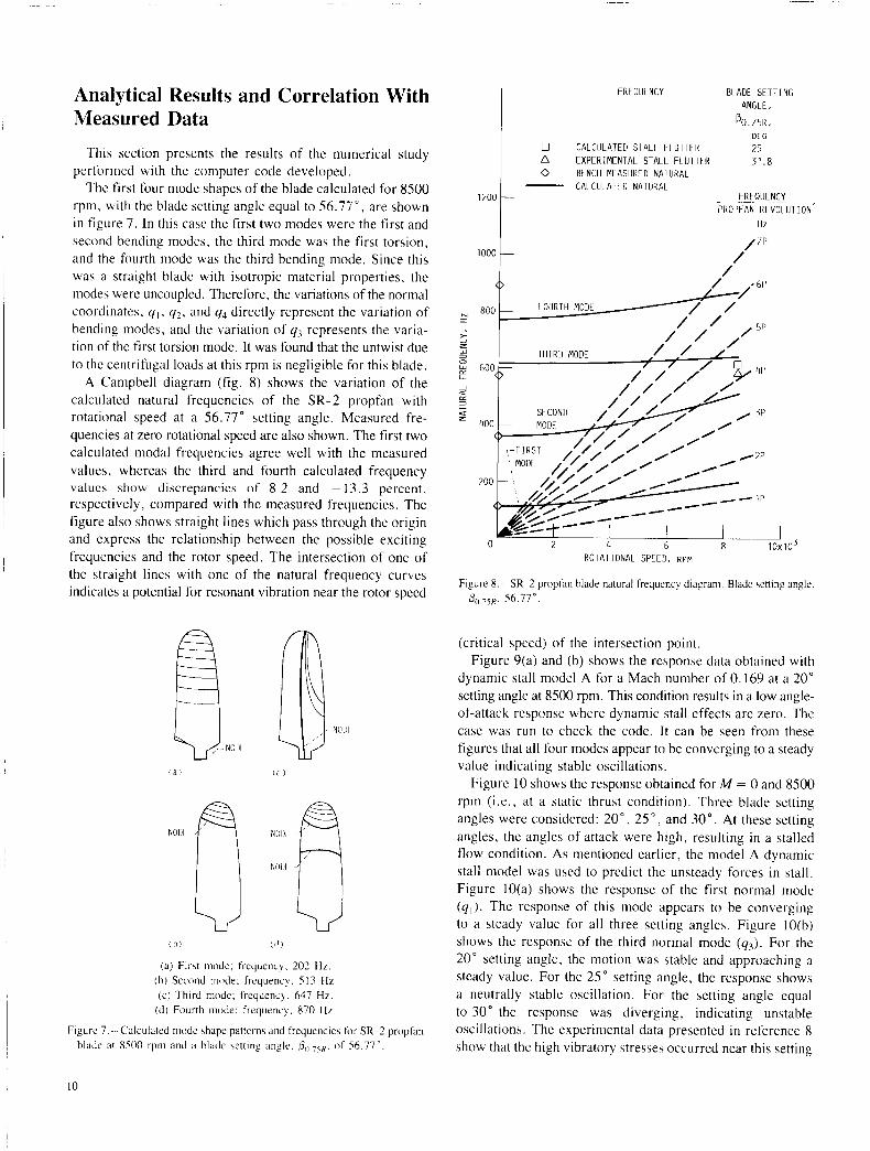
The first four mode shapes of the blade calculated for 8500 rpm, with the blade setting angle equal to 56.77", are shown in figure 7 . In this case the first two modes were the first and second bending modes, the third mode was the first torsion, and the fourth mode was the third bending mode. Since this was a straight blade with isotropic material properties, the modes were uncoupled. Therefore, the variations of the nomial coordinates, q l , q?, and q4 directly represent the variation of bending modes, and the variation of y3 represents the varia- tion of the first torsion mode. It was found that the untwist due to the centrifugal loads at this rpm is negligible for this blade.
A Campbell diagram (fig. 8) shows the variation of the calculated natural frequencies of the SR-2 propfan with rotational speed at a 56.77" setting angle. Measured fre- quencies at zero rotational speed are also shown. The first two calculated modal frequencies agree well with the measured values, whereas the third and fourth calculated frequency values show discrepancies of 8.2 and - 13.3 percent, respectively, compared with the measured frequencies. The figure also shows straight lines which pass through the origin and express the relationship between the possible exciting frequencies and the rotor speed. The intersection of one of the straight lines with one of the natural frequency curves indicates a potential for resonant vibration near the rotor speed
~
(a) First mode; frequency. 203 HI. (h) Second mode: frequency. 513 H z . ( e ) Third mode; frequency. 647 Hz.
(d) Founh mode: frequency. 870 H r .
Figure 7.-Calculated mode shape patterns and frequencies for SR-2 propfan blade a1 8500 rpni and a blade setting angle. p,, ,5N, of 56.77".
(critical speed) of the intersection point. Figure 9(a) and (b) shows the response data obtained with
dynamic stall model A for a Mach number of 0.169 at a 20" setting angle at 8.500 rpni. This condition results in a low angle- of-attack response where dynamic stall effects arc zero. The case was run to check the code. I t can be seen from these figures that all four modes appear to be convcrging to a steady value indicating stable oscillations.
Figure 10 shows the response obtained for M = 0 and 8.500 rpm (i.e., at a static thrust condition). Three blade setting angles were considered: 20", 25" , and 30". At these setting angles, the angles of attack were high, resulting in a stalled flow condition. As mentioned earlier, the model A dynamic stall model was used to predict the unsteady forces in stall. Figure 10(a) shows the response of the first normal mode (y,). The response of this mode appears to be converging to a steady value for all three setting angles. Figure 10(b) shows the response of the third normal mode (q3). For the 20" setting angle, the motion was stable and approaching a steady value. For the 25" setting angle, the response shows a neutrally stable oscillation. For the setting angle equal to 30" the response was diverging, indicating unstable oscillations. The experimental data presented in reference 8 show that the high vibratory stresses occurred near this setting
10
3 0 0 ~ 1 0 - ~ r MODE
- ( a ) 2
-2001
1 oox 10-4 MODE
THIRD ----
-100 0 5.00 10.00 15.00 20.00
TIME. R t . RAD
!a) First and hecond normal mode (b) Third and fourth normal mode.
Figure 9.-Response of dynamic stall model A at 8500 rpni. Mach 0.169. and a blade setting angle. PO 7 5 R , of 20".
angle (31 . S o ) and flow condition ( M = 0). The high stresses are found to not be due to critical speed cross over. The present analysis showed a limit cycle at a 25" setting angle. This condition is taken as a stall flutter condition since the airfoil is at a large initial angle of attack. The calculated frequency of this limit cycle was 617 Hz, which is 3 percent higher than the experimental value of 600 Hz. Note that the calculated
value is for zero structural damping. The experimental data of reference 8 show that the large stresses occurred in the third mode (first torsion). The present analysis also predicted that instability occurred in the third normal mode (q3) , which is the first torsion.
Also note that the response trends for the three setting angles are qualitatively in agreement with those that were calculated in reference 14. In reference 14 a beam structural model and model B dynamic stall with unsteady lift and moment data were used in the analysis. Only static drag data were used since unsteady drag data for the NLR- I airfoil were not available. (A structural damping value of 0.008 was used to see that the response did not diverge at the 30" setting angle.) The
BI AD€ S E T T I N G
ANGLE
75R, DFG
- 70 --- 75 ---- 30
.01
0
.01
( b ) - .02
0 5 10 TIME. 0 1 , RAD
(a) First normal mode. (h) Third nornial mode.
Figure 10 -Re\ponw of dynamic d l model A at Mach 0 and 8500 rpm.
agreement between the present study and that in reference 14 is not surprising since for this blade (SR-2) a beam model would have been sufficient because of zero sweep and isotropic material properties. However, as mentioned earlier, a finite element formulation is more general and applicable to swept propfans made of composite materials. Also thc unsteady drag effects on the response were minimized since the chord was assumed rigid and only a fraction of drag contributed to the normal force on the airfoil.
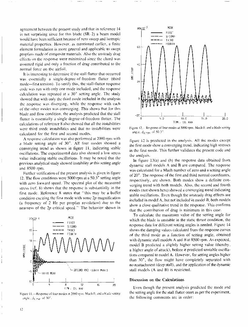
It is interesting to determine if the stall flutter that occurred was essentially a single-degree-of-freedom flutter (third mode-first torsion). To verify this, the stall-flutter response code was run with only one mode included. and the response calculation was repeated at a 30" setting angle. The study showed that with only the third mode included in the analysis the response was diverging, while the response with each of the other modes was converging. This shows that for this blade and flow condition, the analysis predicted that the stall flutter is essentially a single-degree-of-freedom flutter. The calculations of reference 8 also showed that all the instabilities were third mode instabilities and that no instabilities were calculated for the first and second modes.
A response calculation was also performed at 2000 rpm with a blade setting angle of 30". All four modes showed a converging trend as shown in figure 1 1 , indicating stable oscillations. The experimental data also showed a low stress value indicating stable oscillations. It may be noted that the previous analytical study showed instability at this setting angle and 8500 rpm.
Further verification of the present analysis is given in figure 12. The flow conditions were 5000 rpni at a 50.3" setting angle with zero forward speed. The spectral plot of the measured stress (ref. 8) shows that the response is substantially in the first mode. Reference 8 states that "this may be a buffet condition exciting the first mode with sonic 2p magnification (a frequency of 2 Hz per propfan revolution) due to the nearness of the 2p critical speed." The behavior shown in
20x10-3 MODE
F I R S T SFCOND T H I R D FOURTH
--- 15
-10 0 4 8 l ? 16 20
T I M € , Et. RAD
Figurc I I .--Re\ponsc of fou r niodch at ?OOO rpni. Mach 0. and ;I hladc wtting angle. $,, 7 5 K , of 3 0 " .
8 0 ~ 1 0 . ~ MODE
- F I R S T SECOND T H I R D ----
-70 , 0 5 . 0 10.0 15.0 20.0
TIME, !?t, RAD
Figure 12.-Responce t iffour modes at S~xx) rpm. Mach 0. and a blade sclting angle. Po 75R, of 50.3".
figurc 12 is predicted in the analysis. All the modes exccpt the first mode show a converging trend, indicating high stresses in the first mode. This further validates the present code and the analysis.
In figure 13(a) and (b) the response data obtained from dynamic stall models A and B are compared. The response was calculated for a Mach number of zero and a setting angle of 20". The response of the first and third normal coordinates, respectively, are shown. Both modes show a definite con- verging trend with both models. Also, the second and fourth modes (not shown here) showed a converging trend indicating stable oscillations. Even though the unsteady drag effects are included in model A. but not included in model B, both models show a close qualitative trend in the response. This confirms that the contribution of drag is minimum in this case.
To calculate the maximum value of the setting angle for which the blade is unstable in the static thrust condition, the response data for different setting angles is needed. Figure 14 shows the damping values calculated from the response curves of the third mode as a function of setting angle, obtained with dynamic stall models A and B at 8500 rpm. As expected, model B predicted a slightly higher setting value (thereby, a higher angle of attack), before it predicted unstable oscilla- tions compared to model A. However, for setting angles higher than 30", the flow might have completely separated with no reattachment (deep stall). and the application of the dynamic stall models (A and B) is restricted.
Discussion on the Calculations
Even though the present analysis predicted the mode and the setting angle for the stall flutter onset as per the experiment, the following comments are in order:
MODE1
A - B ---
,005
0
- ,005
8 - . n io t 0 20 40 3
( I ) Test data evaluated in reference 8 do not show the stress levels at all gages for the same setting angle. Hence, it was difficult to assess whether there was multimode excitation indicating buffeting. However test data evaluated at NASA Lewis for the same case as in reference 8 showed higher stresses both at the tip bending gage and at the shear gage for the same flow conditions, indicating a niultimodal excitation for the SR-2 blade.
(2) Experimental data showed that the instability moved from a third mode to a second mode instability at higher angles of attack, a phenomena which was not predicted by the present analysis. All the modes showed instability at higher angles.
(3) The validity of the present aerodynamic model at angles of attack where buffet is assumed to have occurred has yet to be investigated.
Conclusions
0 5 10 TIME. R t , RAD
(a) F in t normal mode (b) Third nomial mode
Figure 13 -Re\ponw of model\ A and B at 8500 rpni. M,ich 0. and A blade setting angle, Po 75x, of 20"
\ \
,--\ /
C
30 40 50 60 HLAIIC PITCH ANGLE, DEG
Figure 14.-Variation of logarithmic decrement with setting angle at 8503 rpm and Mach 0.
The stall flutter response of an unswept SR-2 propfan wind- tunnel model was studied with a semiempirical dynamic stall model. The results were compared with available experimental and analytical data. The following conclusions are drawn from this study.
1. The Gormont dynamic stall model (model A), where only a correction to angle of attack is used, qualitatively predicts the same trend as that observed in experiments. The predictions of this model agree well with those predicted by the Gangwani dynamic stall model (model B), a model based on the synthesization procedure.
2 . Both models are conservative in predicting the setting angle at which stall-flutter occurred in the experiment.
3. Even though the present study and that of reference 14, where a beam model is used, predicted the same behavior; a finite element formulation is more general. particularly for applications to swept propfan blades with composite materials.
The following suggestions are made to improve the analysis: 1. Experimental static and dynamic stall data for NACA 16
series airfoils that are employed for propfans should be generated and used in the analysis.
2 . Cascade corrections to isolated airfoil lift, drag, and moment coefficients should be included.
3. A more refined induced velocity calculation method is required especially at static thrust conditions.
4. For a more direct comparison with experimental data, a stress calculation module should be developed and included in the code.
5 . The formulation and the computer code should be checked for swept blades and should be applied to study the response with blades made up of composite materials.
6. The analysis should include a complete nonlinear analysis both in structural modeling and aerodynamic modeling instead of a linearized structural model and nonlinear aerodynamic model as was done here.
Appendix A Symbols
D' d
disk area points on the reference line
4, ith generalized (normal) coordinate R rotor radius
distance between reference axis and the quarter Re Reynold number
static lift curve slope
number of blades T thrust semichord [TI J , [ T,] transformation matrices full chord t time
chord r position of a mass point (eq. (7))
sign ( ) sign of ( ), either positive or negative
unit vectors along the Xt, Yi.,Zr axes aerodynamic drag coefficient aerodynamic lift coefficient design lift coefficient aerodynamic moment coefficient about the
aerodynamic moment coefficient about the
drag diameter of the propfan distance between the reference axis and the
width of the strip force component in the X,' direction (eq. (20)) force component in the Zt direction (eq. (20)) generalized force at the jth strip plunging degree of motion. positive downward contribution of ith modal deflection to plunging
unit vectors along the XB,UB,ZB axes unsteady aerodynamic empirical factor (eq. (17)) reduced frequency based on semichord aerodynamic lift force Mach number aerodynamic moment moment about the reference axis (eq. (20)) generalized mass in the ith normal coordinate number of normal modes number of blade segments rotor speed in revolutions per second normal vector frequency of n Hz per propfan revolution generalized aerodynamic force in the ith normal
reference axis
quarter chord
three-quarter chord
motion
coordinate
airfoil thickness to chord ratio chordwise, tangential, and normal velocities at
a section unsteady (perturbed) displacements at a point steady displacements at a point
steady induced velocity
resultant velocity, J U ; i- U ; relative velocity vector
free-stream velocity basic (rotating) coordinate system inertial coordinate system local coordinate systcm coordinates of a point in the basic coordinate
y coordinate of jth strip instantaneous angle of attack angle of attack for zero lift
effective angle of attack (eq. (16)). effective angle of attack for lift (eq. (18)). contribution of ith modal deflection to pitching
pitching degree of motion, positive (nose up) shaft (propeller tilt) angle of attack static stall angle mean or initial angle of attack amplitude of oscilliation blade pitch setting angle at 0.75 radius
system
motion
setting angle relative to the one at 0 .75 radius stall delay function (eq. (19)) incremental dynamic stall angle (eq. (15)) critical damping (structural) ratio in the ith mode air density
4 inflow angle $ Rr , nondimensional time n blade rotational speed, rad/sec
w, W rotational vector (eq. (5))
a( )/ay system
(‘1 d( )ldt (“1 d2( )ldt2
coupled frequency in the ith mode -
derivative with respect t o y in the local coordinate
I
I Subscripts: I
a airflow B basic b blade
I L P M
111
re1 rot s
inertial lift local moment due to blade motion relative due to blade rotation steady
Superscripts: T transpose
vector
unit vector
-
I
15
Appendix B Calculation of Unit Vectors
This appendix presents the calculation of unit vectors of the X,,, &,,Z,# coordinate system, and thereby the calculation of the transformation matrix, [ T2], relating the basic coordinate system to the local coordinate system.
Let A,(.r,x,:) represent points on the reference line, where the unit vectors are to be calculated. The index i ranges from 1 to the number of strips the blade is divided into. Consider another adjacent point A , + , ( x + Ax,? + Ay,z + Az).
The unit vector i, tangent to the reference line at the point A, and positive from root to tip, is given approximately as
where
As = d(A.rY + (Ai,)? + (A:)' (B2)
and i, j , and k are the unit vectors in the basic coordinate system.
The chord line vector i. is a line that lies in a plane perpendicular to the tangent vector i. Let this plane intersect the trailing edge line of the blade at point B,. The direction of E is obtained by joining points A, and B, directed towards B,. The unit vector
^ ^
is given by
Then the normal vector il at point A, is given by the cross product of vectors and i: that is,
This procedure of finding the transformation matrix between the local and the basic coordinate systems automatically accounts for the curvature of the reference axis. Summarizing, the chordwise, tangent. and normal unit vectors at any point A, arc given by
Then the transformation between the local and basic coordinate system is given by
or
16
Appendix C Calculation of Steady Induced Velocity
This appendix presents the equations to calculate steady induced velocity Vi (see eq. (4)) using the combined momentum-blade element theory. A discussion on other methods of calculating induced velocity is also included.
In momentum theory, the propfan is approximated by an infinitely thin actuator disk across which the static pressure increases discontinuously. The assumptions inherent in this model (ref. 20) are (1) the velocity is constant through the disk, (2) the pressure is uniform over the disk, (3) rotation imparted to the flow as it passes through the propfan is neglected, (4) the flow passing through the propfan can be separated from the rest of the flow by a well-defined stream tube, and (5) the flow is incompressible. Applying the Bernoulli equation ahead and downstream of the propfan, it can be shown that the thrust is given by
where V , is the free-stream velocity, V, is the induced velocity, p, is the air density, A is the disk area, and CY, is the shaft angle of attack. This can be interpreted as thrust equal to mass flux through the propfan, p,A ( V , cos a, + V , ) , times the total increase in the velocity of the flow (2VJ.
The thrust produced by the propfan can also be calculated from the known aerodynamic properties (er and cd) of the propfan blade. Figure 15 shows the cross section of a blade with velocities influencing the element. The pitch angle 0, of the section is defined relative to the zero lift line of the airfoil section. The contribution of one blade element to the thrust Tis
dT = dL cos($ + ai) - dD sin($ + ai) (C2)
where dL and dD are the differential lift and drag forces, respectively, and cyi is the induced angle of attack due to the
THRUST
i j l R E C T ' O N CHORD ,
cosos
Figure 15 .-Velocity and force diagram for propeller blade element
induced velocity Vi. The lift and drag forces, dL and dD, are given by
1
2 dD = - p,Vi c(cr) dr
Here cr is given by aol(P - 4 - a,), where uol is the linear lift curve slope, cd can be obtained as a function of cy, and c is the chord.
Assuming a, and drag to lift ratio to be small, dT for B number of blades is given by
By applying equation (CI) to the differential annulus, the elemental thrust is given by
Equating equation (C4) to (C5) yields a quadratic equation for V,, from which V, can be calculated.
Note that other blade element theories differ from the momentum-blade element theory principally in the way in which the wakes are modeled. The basic vortex theory describes the wake by a series of cylindrical vortex sheets representing the radial variation of circulation, implying an infinite number of blades.
Goldstein (ref. 21) assumes helecoidal surfaces for each blade. The helecoids are assumed to move downward uni- formly at the average momentum velocity, and the effects of wake contraction, viscosity, and nonuniform downwash on the wake shape are neglected. This theory is inadequate when used to analyze propfans with increased blade loading, tip Mach number, and number of blades. Also this method is inadequate to predict static (static thrust condition) performance where wake contraction and tip rollup must be taken into account. Wake contraction will position the vortex generated by each blade tip closer to the tip path plane than is assumed in the Goldstein analysis. Close proximity of the tip vortex to the following blades causes severe local inflow distribution due to high rotational velocities with the vortex. These rotational velocities reach levels as high as 50 percent of the blade tip speed.
17
I Various methods-namely. lifting line, lifting surface, induced velocity extrapolated from low-speed flight analysis vortex lattice method (VLM), and computational fluid is used. (See refs. 21 to 24 for further details.) These methods dynamics (CFD)-have developed to account for wake can be used for swept propfans. When applying combined geometry and wake distortion for low- to high-speed flights. momentum-blade element theory, the blade sections have to For static thrust conditions, either a prescribed wake geometry be taken along the streamline. from experimental observation is used in the analysis or the
Appendix D Effect of Airfoil Static Data Variation on the Dynamic Stall Response
To understand the effect of airfoil static data above stall on the stall-flutter response, one can make calculations with prescribed static data above stall, and the variation in response can be studied. However, for a response study, cf, cl,ll.;4. and cd cannot be varied independently since they are interrelated. However, dynamic stall loops (dynamic l i f t , moment, and drag versus angle of attack) can be obtained with independent variation of static lift, drag, and moment coefficients above stall, and some inference can be drawn. In stall flutter, the negative aerodynamic damping is mostly from the dynamic moment loop. So in the present study the static clnl.14 is varied and the dynamic moment loops are studied. Three cases are studied as shown below and in figure 16.
Case-A Moment Coefficient
This case is a curve-fitted expression for the static moment data given in the G400PROP program (ref. 14) at the 75-percent-radius location for a Mach number of 0.7,
~ ' ~ ~ ~ ~ / 4 = -0.035 - O . O O ~ * C Y for CY < 6"
c ' ~ ~ ~ ~ , ~ = -0,053 - 0.024*(cr - 6.0) for 6" < CY < 10"
cClnl4 = -0,149 - O.O085*(a - 10) for CY > I O "
Case-B Moment Coefficient
c,,,,,~ = -0.553 - O.O15(a - 6) for CY > 6"
Case-C Moment Coefficient
c , , , , / ~ = -0.553 - 0.010(a - 6) for CY > 6"
Figure 17 shows the dynamic cmCl4 loops obtained with static-stall moment data assumed as above. The angle-of-attack variation is given by CY = 5" + 3" sin(wt) at a reduced frequency of 0.05 and for a Mach number of 0.7. The dynamic loops are indicative of the energy transfer from the flow to the structure. In figure 17, the dynamic loop obtained with case-A static data shows a large hysteresis loop above stall, which means that negative work is being done on the structure. This may lead to a net negative damping at certain flow conditions. The area of the loop reduces by about half with case-B assumed static data. With the case-C assumed static data no negative loop is obtained, indicating there is no negative work on the structure. This shows that inaccil,.ate static data above stall can lead to positive or negative damping, leading to stable or unstable response.
0x104 r -500
F
E -1500
W
6 \' u I \
ANGLE OF AlTACK. a
Figure 16 -Variation o f \tatic moment coefficient with angle of attack.
D3
4.0 6.0 8.0 10.0 ANGLE OF AlTACK. a
Figure 17.-Variation of dynamic moment coefficient with aaaumed static moment coellicient at Mach 0.7 and reduced frequency. X , of 0.05; N = 5 + 3 sin ks: model A dynamic sta l l .
19
References
I . Mehmed. 0.. et al : Bending-Torsion Flutter of a Highly Swept Advanced Turboprop. NASA TM-82975. 1981.
2 Mehmed, 0.: and K a n . K.R.V.: Experimental Clas\ical Flutter Rewlts o f a Compo\ite Ad\anced Turboprop Model. NASA TM-88792. IYX6.
3 . Kara. K.R.V. , et al.: Analytical Flutter Investigation o f a Composite Propfan hlodel. 28th Structures, Structural Dynamics and Materials Conference. Part 2A. AIAA. 1987. pp. 84-97. (NASA TM-88944).
4. Kaza, K.R.V. . et al.: Analytical and Experinlental Investigation of Mistuning in Propfan Flutter. 28th Structures, Structural Dynamics and Material5 Conference. Part 2.4. AIAA. 1987, pp. 98-110. (NASA TM-889.59).
5 . Reddy. T.S R; and Kaza. K.R.V.: A Comparative Study of Some Dynamic Stall hlodcl$. NASA TM-88917. 1Y87.
6. McCroskey. W.J . : The Phenomenon of Dynamic Stall. NASA TM-81264. 1981.
7 . Galbraith. R.A.M; and Vezra. M: Methods of Predicting Dynamic Stall. Wind Energy Conversion 1986, R.A.M. Galbraith, et al. , eds.. Mechanical Engineering Puhllcations. London. 1986. pp. 263-272.
8. Smith. A.F : Analyis and Te\t Evaluation of the Dynamic Stability of Three Advanced Turboprop Models at Zero Forward Speed. (HSER- I 1054. Hnmilton Standard; NASA Contract NAS3-22755) NASA CR-175025. 1985.
9. Smith. A .F . : Analy\i\ and Test Evaluation of the Dynanlic Rcspon\e and Stahility 01. Tliree Advanced Turhoprop Models at Low Forward Speed. (HSER-I 105.5. Hamllton Standard: NASA Contract NAS3-22755) NASA CR-175026, 1985.
IO. Gormont. R.E. : A Mathematical Model of Unsteady Aerodynamics and Radial Flou for Application to Helicopter Rotors. USAAMRDL- TR-72-67. May 1973. (Avail. NTIS. AD-767250).
1 1 . Gangwani. S.T. : Synthesired Airfoil Data Method for Prediction of Dynamic Stall and Unsteady Airloads. NASA CR-3672. 1983. (Also \ee; Prediction of Dynamic Stall and Unsteady Airloads for Rotor Blades. I . Am. Helicopter Soc.. vo l . 27. no . 4, Oct. 1982, pp. 57-64).
12. Tran, C.T. : and Petot. D. : Semi-Empirical Model for the Dynamic Stall of Airfoils in View of the Application to the Calculation of Responses of a Helicopter Blade in Forward Flight. Vertica, vol. 5 . no. I. 1981, pp. 35-53.
13. Steinman, D.B.: Aerodynamic Theory of Bridge O\cillations. Proc. Ani. S(ic. Civ. Eng.. vol. 7.5, no. X, Oct. 1949. pp. 1147-1184.
14. Bielawa, R.L.. et al. : Aeroela\tic Analysis of Propeller\ NASA CR-3729. 1983.
16. Egolf. T.A. . et al.: An Analysis for High Speed Propeller-Nacellc Aerodynamic Performance. Vol. I-Theory and Initial Application: Vol. 2-User's Manual lor the Computer Program. (R79-912Y49-14. United Technologies Re\earch Center: NASA Contract NAS3-2096 I )
NASA CR-169450. NASA CR-169451. 1979. 17. Mak\yniuk. C .M: and Watwn. S.A. . A Conlputer Program for
Ehtiniating the Aerodynainic Charactenstic\ of NACA Ih-Sene\ Airfoil\. NASA TM-X.5696, 1983.
18. Bathe. K.J.: and Wilson. E.L. : Numerical Method\ in Finite Element Methods. Prentice Hall. 1976.
19. Stelko. G.I..; and Jeracki. R.J.: Wind Tunnel Results of Advanced Hlgh S y e d Propeller\ in the Takeoff, Climb, and Landing Operating Regime\. AIAA Paper 8.5-125'). July 19x5. (NASA TM-87054).
20. McCormick, B.W.: Aerodynanlics, Aeronautics, and Flight Mechanics. John Wiley & Sons. 1979. pp. 343-369.
21. Gold\tein. S . On the Vt)rtcx Theory of Screw3 Propellers. Proc. R Soc. London Ser. A, vol
22. Miller. C.J. . Optimally I h i g n e d Propeller\ Constrained by Noise. Ph 11. Thesis. Purdue Univervty, 1983.
23. Williams, M.H. ; and Huang, C.C. : Three Dimensional Unsteady Acrodynamics and Aeroclastic Re\ponce ol Advanced Turboprop\. 27th Structures. Structural D y n a r n u and Materials Conference. Part 2. AIAA, 1986, pp. 116-124.
24. Boher. L.J. ; Chaussec. D.S.: and Kutler. P . : Prediction of High Speed Propeller Flow Fields U\ing a Three Dimensional Euler Analy\i\. AIAA Paper 83-01R8, Jan. 1983. (NASA TM-8306.5).
T.S.R. Reddy, The University of Toledo, Department of Mechanical Engineering, Toledo, Ohio 43606 and NASA Resident Research Associate; K.R.V. Kaza, NASA Lewis Research Center.
9. Security Classif. (of this report)
Unclassified
16. Abstract
The time-history response of a propfan wind-tunnel model with dynamic stall was studied analytically. The response obtained from the analysis was compared with available experimental data. The governing equations of motion were formulated in terms of blade normal modes calculated using the COSMIC-NASTRAN computer code. The response analysis considered the blade plunging and pitching motions. The lift, drag, and moment coefficients for angles of attack below the static stall angle were obtained from a quasi-steady theory. For angles above static stall angles, a semiempirical dynamic stall model based on a correction to the angle of attack was used to obtain lift, drag, and moment coefficients. Using these coefficients, the aerodynamic forces were calculated at a selected number of strips, and integrated to obtain the total generalized forces. The combined momentum-blade element theory was used to calculate the induced velocity. The semiempirical stall model predicted a limit cycle oscillation near the setting angle at which large vibratory stresses were observed in an experiment. The predicted mode and frequency of oscillation also agreed with those measured in the experiment near this setting angle. The results also correlated well with the other published data that used a semiempirical dynamic stall model based on a synthesized procedure.
20. Security Classif. (of this page) 121. No of y 22. Price'