Dynamic Testing of Permanent Magnet Synchronous Machines Sebastian Hall Licentiate thesis Division of Industrial Electrical Engineering and Automation Department of Biomedical Engineering 2016
Transcript
Dynamic Testing ofPermanent Magnet
Synchronous Machines
Sebastian Hall
Licentiate thesisDivision of Industrial Electrical Engineering and Automation
Department of Biomedical Engineering
2016
Division of Industrial Electrical Engineering and AutomationDepartment of Biomedical EngineeringFaculty of EngineeringLund UniversityBox 118221 00 LundSWEDEN
The rst thank you goes out to Professor Alaküla for realizing thisproject. The support and motivational talks have been phenomenal.The second thank you is for Associate Professor Reinap for the avail-ability and philosophical perspective on engineering and life. Fantastic.My research group crew denitely deserves a big salute for the helpfuldiscussions. Then of course, I cannot forget to mention the one and onlyGetachew Darge, king of the workshop, savior of the day. Also, Carinaand Ulrika, the queens of administration, have my sincerest gratitudefor saving me on several occasions. Actually, thanks to the whole divi-sion of Industrial Electrical Engineering and Automation. I am sorryif I missed a coee week; if so, it was not on purpose. Finally, I mustgive credit to the ELDRIVET group for the support and interestingget-togethers.
Outside of work I thank my family and friends for putting up withoccasional whining due to motivational downswings. You are the bestand I would probably pass away in an instance if you went away. Tack!
Abstract
This thesis presents a method to test and characterize Permanent Mag-net Synchronous Machines (PMSMs) called the Dynamic Test Method(DTM). In contrast to traditional methods, the DTM tests machineswithout a brake or a locking mechanism for the test object's rotor. In-stead, the moment of inertia of the rotor shaft limits the mechanicaldynamics while a voltage source imposes torque producing currents onthe stator windings of the machine. While a specic predened currentproduces a torque which accelerates and brakes the machine, a data ac-quisition system samples measurements of the phase currents, the phasevoltages and the rotor position with a high sampling frequency. A post-processing algorithm then derives the performance of the machine forthe specic phase currents from the sampled data.
The main focus of this work lies on the magnetic model identication.The magnetic model describes the relationship between the currentsand the linked magnetic ux in a machine. The model gives feedbackto designers, provides the air-gap torque characteristics of the machineand helps with the implementation of optimal eld-weakening control.Through equations from the equivalent model of the PMSM, the ob-tained data yields the linked magnetic ux as a function of the testcurrents. The method derives the ux from measurements from boththe motor and the generator regime of the machine, and can thereforeobtain the ux without knowledge of the stator winding resistance. Thisalso makes it possible to disregard the iron losses inuence on the uxlinkage. Experimental results show a good match between the DTMtest results and results from a traditional constant speed method. Theexperiments show that the temperature has little eect on the DTMresults compared to the constant speed method.
iv
The DTM also provides the torque characteristics of a PMSM. Themethod derives the air-gap torque from the linked magnetic ux andcurrents, and also the rotor shaft torque from the acceleration and mo-ment of inertia. To derive the rotor shaft torque, this work presentsa method to obtain the rotor shaft moment of inertia from a pendu-lum and ywheels. Experimental measurement results from both themotor and generation operation show good consistency of the torquemeasurements. Furthermore, the average values between the generatorand motor tests show that the moment of inertia of the rotor shaft canbe obtained solely from the dynamic tests. This makes it possible toderive the eciency and losses of the machine without a torque sensoror knowledge about the moment of inertia of the rotor shaft.
In addition to the magnetic model identication and the torque perfor-mance characterization, this thesis also outlines a theoretical frameworkfor eciency derivation and loss separation of a test object. The e-ciency tests provide a fast evaluation of the machine which can compli-ment the more detailed tests in a conventional test setup. The methodderives the eciency from the electric power, which it calculates fromthe voltages and currents, and the mechanical power, which is calcu-lated from the acceleration, speed and moment of inertia of the rotorshaft. Experimental tests show that there still exist question marks re-garding the performance of the method. The rotational speed of the testobject does not reach the expected, and the eciency results are low.Even so, the results give a steady foundation for future research.
Nomenclature
α Bandwidth of PI controller
αe Voltage error factor
β Converter semi-conductor voltage drop error factor
cos(φ) Power factor
δ State of a converter leg
η Eciency
ωex Resolver excitation frequency
ωmax(isd, isq) Maximum speed for a specic current combination in the
dq frame
ωb Cut-o frequency for the moving average lter
ωm Rotor shaft rotational frequency
ψm Linked permanent magnet ux
Ψsdq(s) dq linked ux vector in the frequency domain
vi
ψ
(iψd ,i
ψq
)dq Linked magnetic ux in the dq frame
ψ(isd,i
sq)
dq Mean value of the linked ux from the motor and the generatorregion
θ Rotor angular position
θidq dq current vector angle in respect to the d axis
θudq dq voltage vector angle in respect to the d axis
~ψsdq dq linked magnetic ux vector in polar coordinates
~isdq dq current vector in polar coordinates
~usdq dq voltage vector in polar coordinates
ci Integral gain for the Direct Current Control algorithm
iψdq Equivalent current which gives rise to linked ux
ifdq Equivalent iron loss current in the dq frame
isdq Stator winding currents in the dq frame
Isdq(s) dq current vector in the frequency domain
J Rotor shaft moment of inertia
Jf Fly-wheel moment of inertia
vii
Jp Pendulum moment of inertia
k Transformation scaling factor
Ke Eddy current loss coecient
Kf Mechanical friction coecient
Kh Hysteresis loss coecient
ki PI controller integral gain
kp PI controller proportional gain
Kexc Excess loss coecient
L Stator winding inductance (Varies with the rotor position)
p Number of pole pairs
Pm Mechanical power
Pe Electric power
Rf Equivalent eddy current loss resistance
Rs Stator winding resistance
Tmag Mean air-gap torque from the motor and the generator regime
T ext External rotor shaft torque
Tmecloss Mechanical loss torque
viii
Tag Air-gap torque
Tloss Torque due to iron losses and mechanical losses
Trs Rotor shaft torque
uresd The direct resolver signal
uresq The quadrature resolver signal
uabc Phase voltages
UN Voltage from converter phase leg to DC-link minus
Un Voltage from converter phase leg to machine neutral
uαβ Voltage in the αβ frame
Udc DC-link voltage
udq Voltage in the dq frame
U sdq(s) dq voltage vector in the frequency domain
Udrop Voltage drop over semi-conductor components in the converter
List of Figures
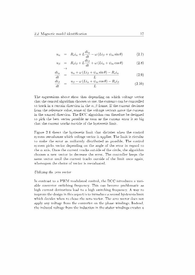
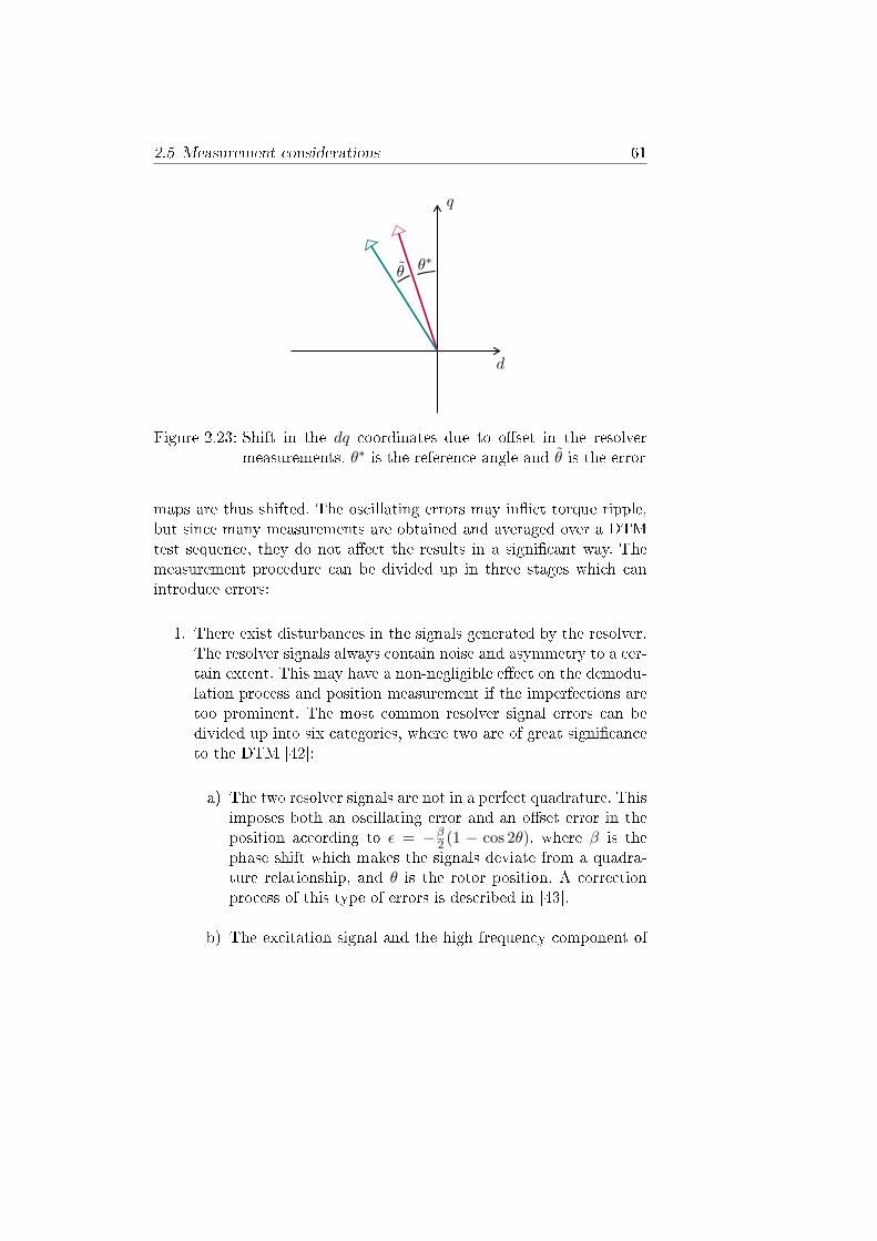
2.1 Coordinate systems of a PMSM . . . . . . . . . . . . . . 112.2 Equivalent circuit of the PMSM in the dq reference frame 122.3 Dynamic test sequence for magnetic model derivation . . 142.4 Converter voltage vectors together with the hysteresis
limit, shown in blue, and the reference value, shown as alled blue circle in the middle of the hysteresis limit. Thelimit is designed so the voltage vector which is chosentracks the current towards the reference; for example, ifthe measured current is far right of the reference value,the algorithm applies vector (4) . . . . . . . . . . . . . . 16
2.5 Voltage vectors, current derivatives and hysteresis limits 182.6 Flowchart of the direct current control in αβ coordinates.
The box after the subtraction represents a transforma-tion from Cartesian to polar coordinates . . . . . . . . . 19
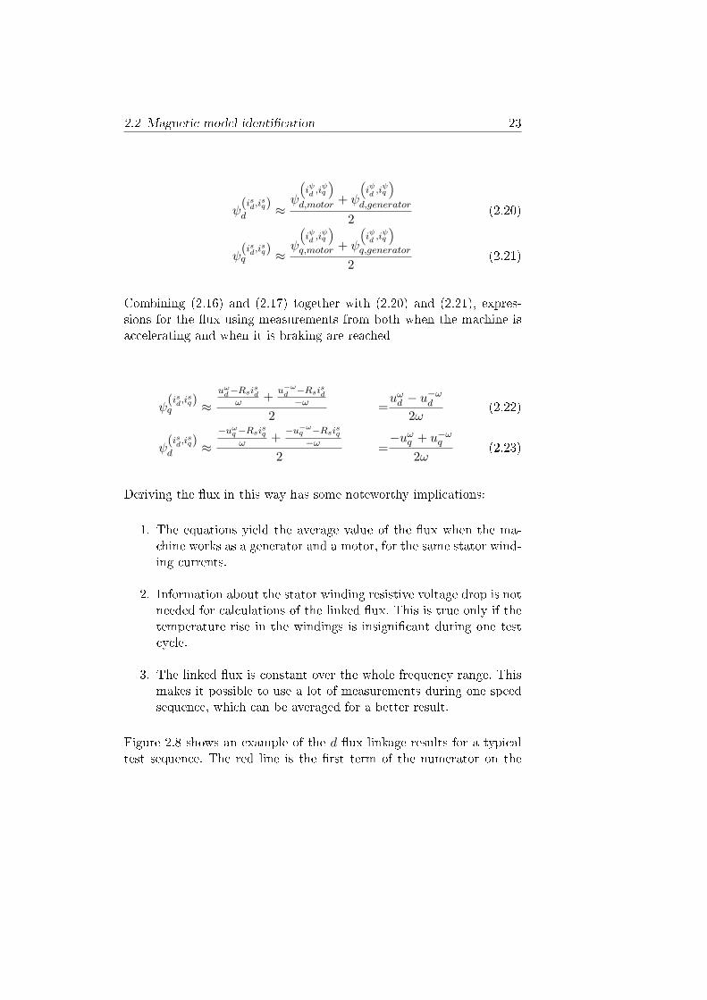
2.7 Complete algorithm with moving hysteresis limits . . . . 202.8 Flux derivation using the dynamic test method. The red
line is the rst term in the denominator of the right handside in (2.22), the blue line is second, and the green isthe result from the total expression . . . . . . . . . . . . 24
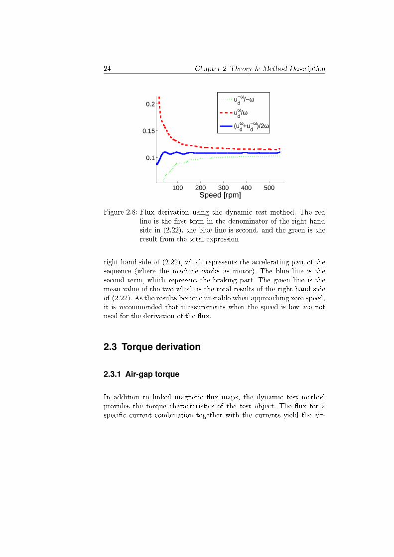
2.9 Mechanical torque derivation using the dynamic test method.The blue line is when the machine works as generator,the red line when it works as a motor, and the green lineis a mean value between the two . . . . . . . . . . . . . 28
2.10 Typical ywheels and a pendulum which can be used toderive the rotor moment of inertia . . . . . . . . . . . . 29
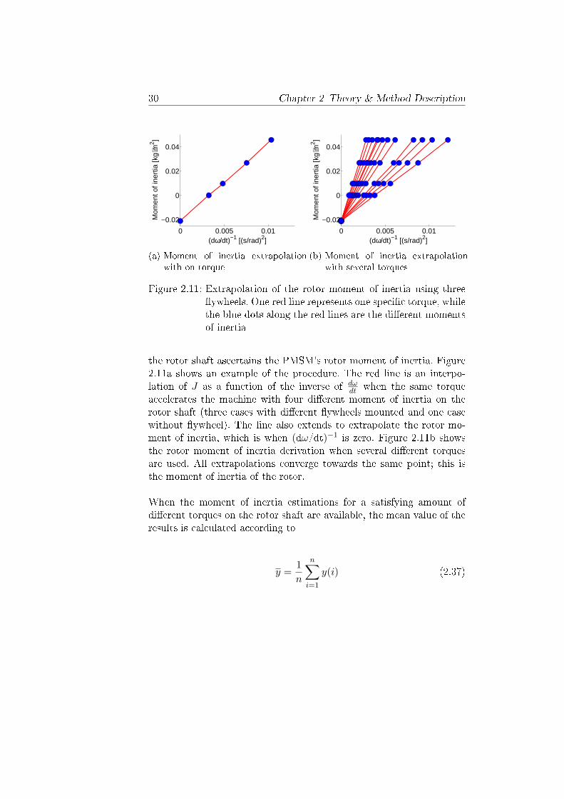
2.11 Extrapolation of the rotor moment of inertia using threeywheels. One red line represents one specic torque,while the blue dots along the red lines are the dierentmoments of inertia . . . . . . . . . . . . . . . . . . . . . 30
2.12 Flowchart of the eld oriented vector controller . . . . . 35
x List of Figures
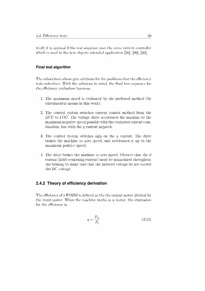
2.13 Updated owchart of the eld oriented vector controller 382.14 Constant torque lines and speed limit lines. Many current
combinations yield the same torque which means that theeciency is dependent on the torque control algorithm . 41
2.15 High resolution torque matrix . . . . . . . . . . . . . . . 422.16 Graphical explanations of steps to reach the eciency as
a function of torque . . . . . . . . . . . . . . . . . . . . 432.17 One fundamental period of voltage and current measure-
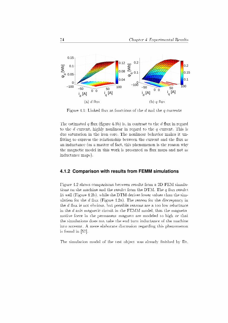
4.1 Linked ux as functions of the d and the q currents . . . 744.2 Comparison between the magnetic ux linkage model de-
rived by the dynamic test method (blue surface) andfrom FEMM simulations (yellow surface) . . . . . . . . . 75
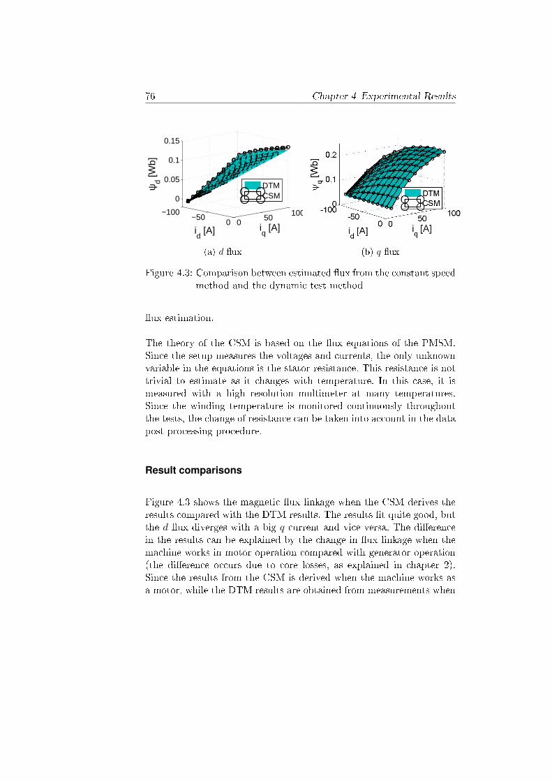
4.3 Comparison between estimated ux from the constantspeed method and the dynamic test method . . . . . . . 76
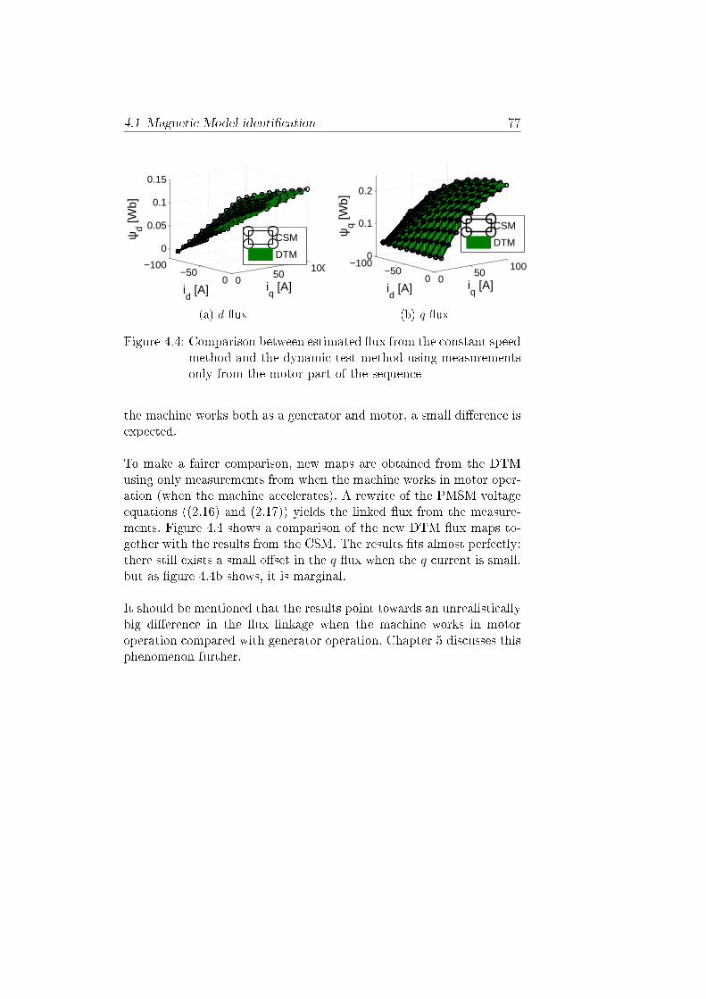
4.4 Comparison between estimated ux from the constantspeed method and the dynamic test method using mea-surements only from the motor part of the sequence . . 77
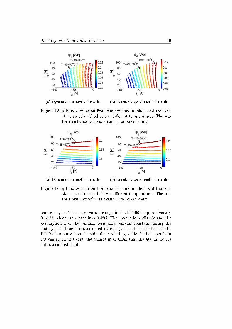
4.5 d Flux estimation from the dynamic method and theconstant speed method at two dierent temperatures.The stator resistance value is assumed to be constant . . 79
List of Figures xi
4.6 q Flux estimation from the dynamic method and the con-stant speed method at two dierent temperatures. Thestator resistance value is assumed to be constant . . . . 79
4.7 Resistance progression of winding temperature sensorduring one test cycle . . . . . . . . . . . . . . . . . . . . 80
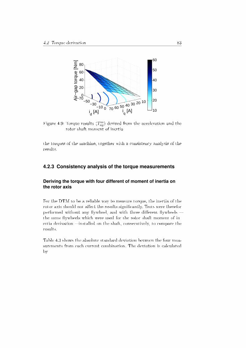
4.9 Torque results (Tmag) derived from the acceleration andthe rotor shaft moment of inertia . . . . . . . . . . . . . 83
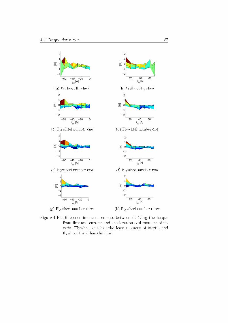
4.10 Dierence in measurements between deriving the torquefrom ux and current and acceleration and moment ofinertia. Flywheel one has the least moment of inertiaand ywheel three has the most . . . . . . . . . . . . . . 87
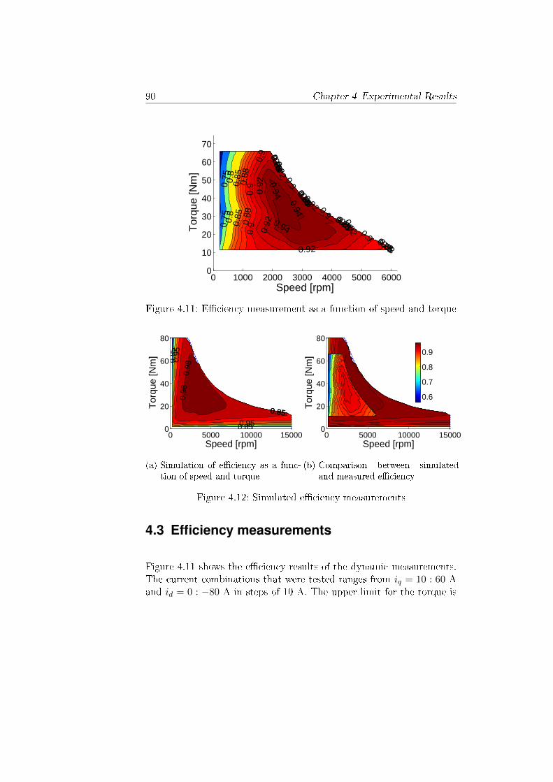
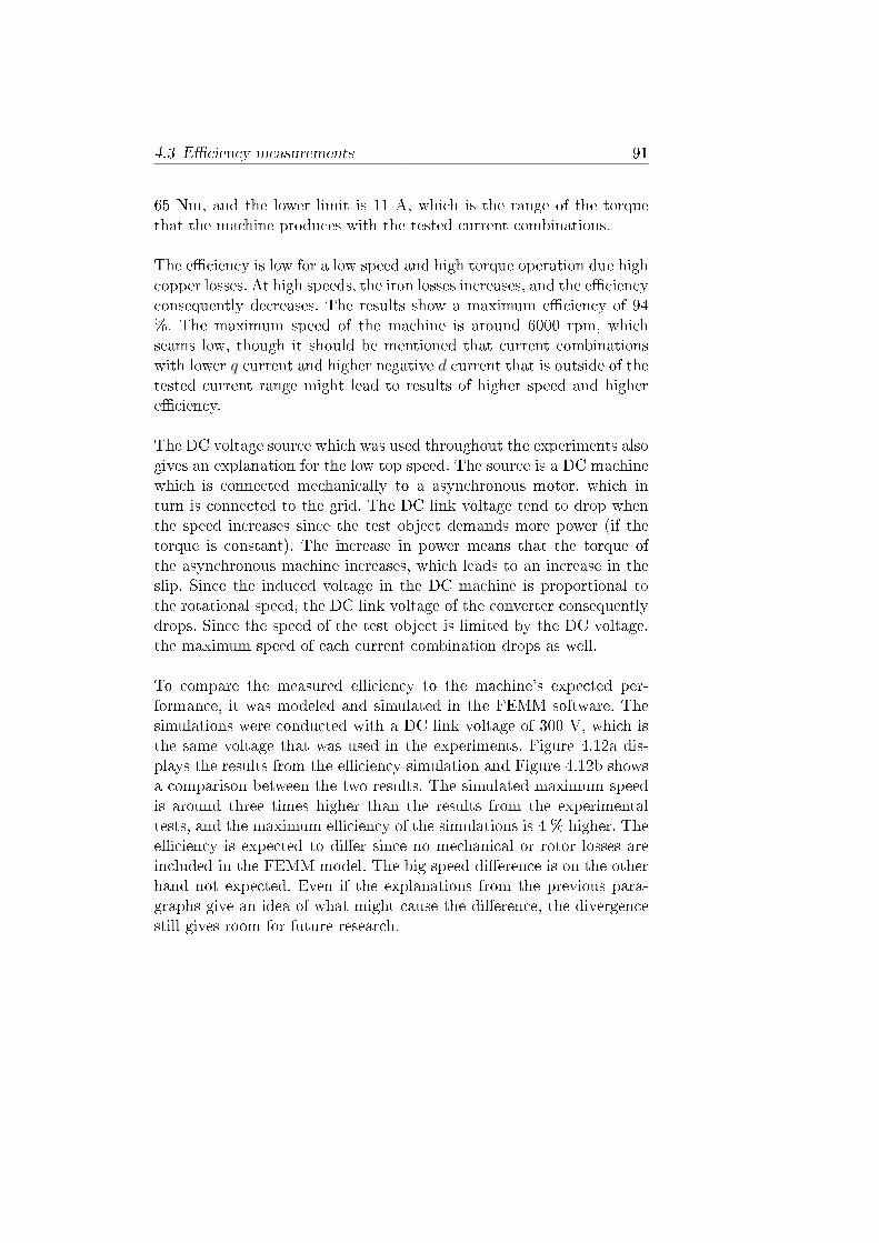
4.11 Eciency measurement as a function of speed and torque 904.12 Simulated eciency measurements . . . . . . . . . . . . 904.13 Power factor with dierent current combinations, derived
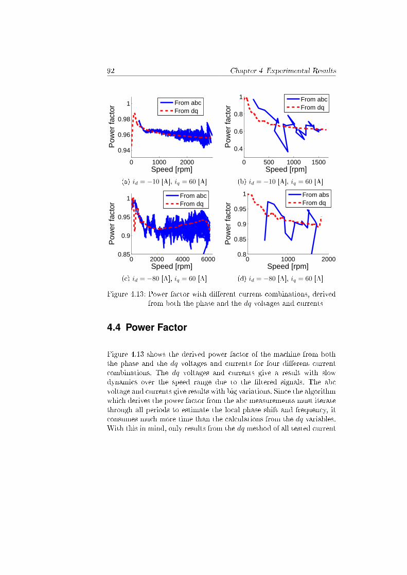
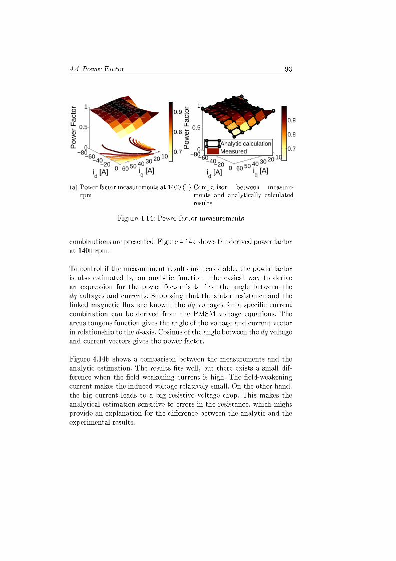
from both the phase and the dq voltages and currents . 924.14 Power factor measurements . . . . . . . . . . . . . . . . 93
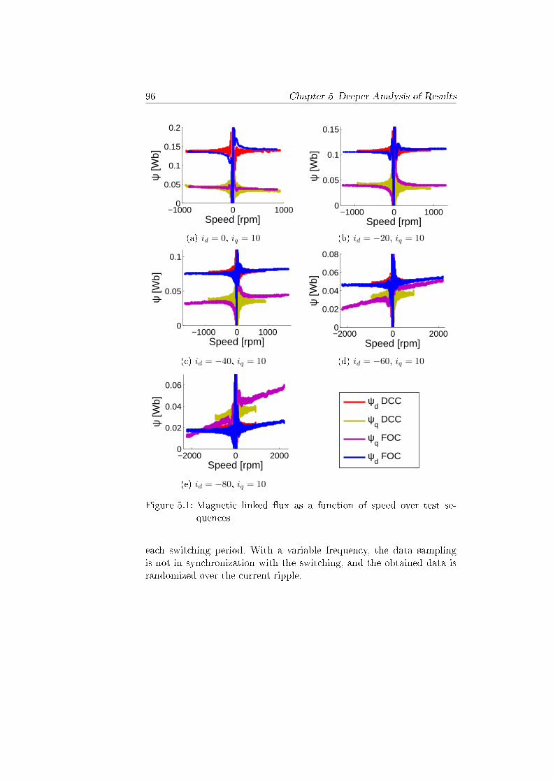
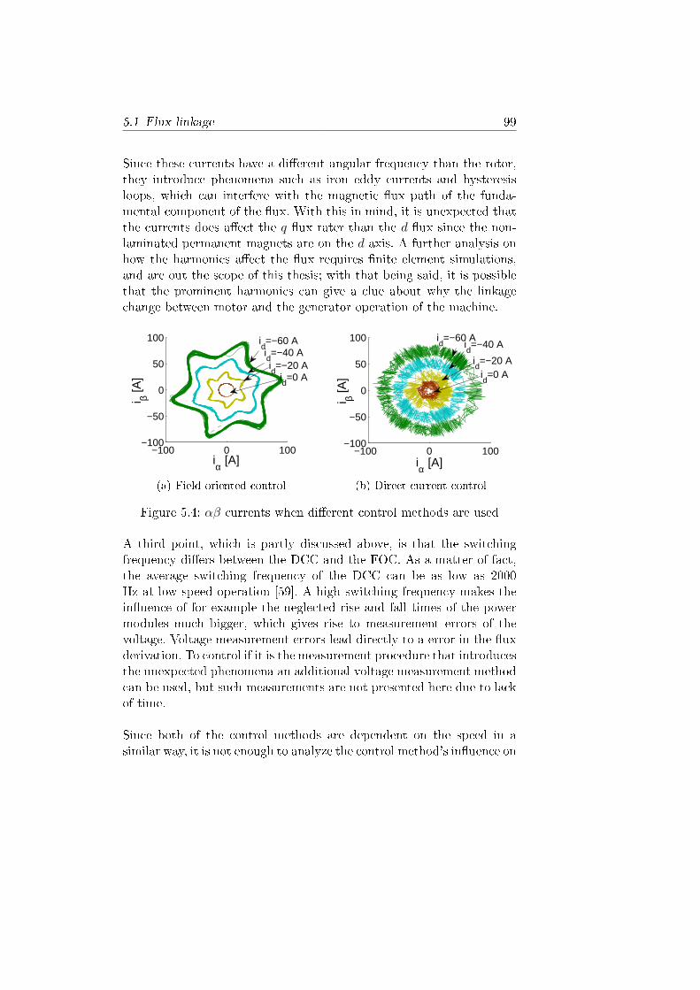
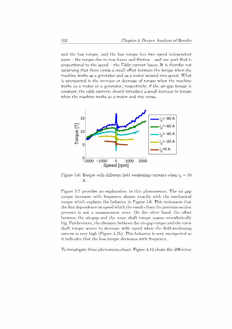
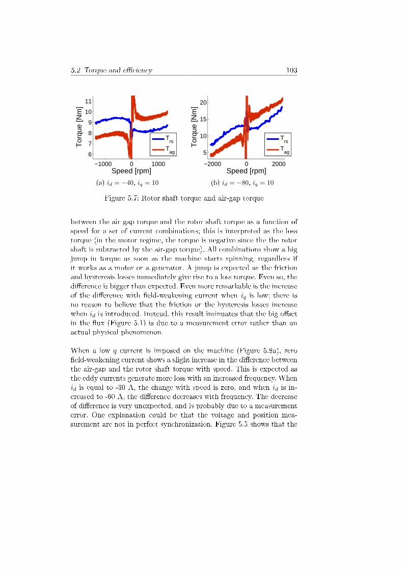
5.1 Magnetic linked ux as a function of speed over test se-quences . . . . . . . . . . . . . . . . . . . . . . . . . . . 96
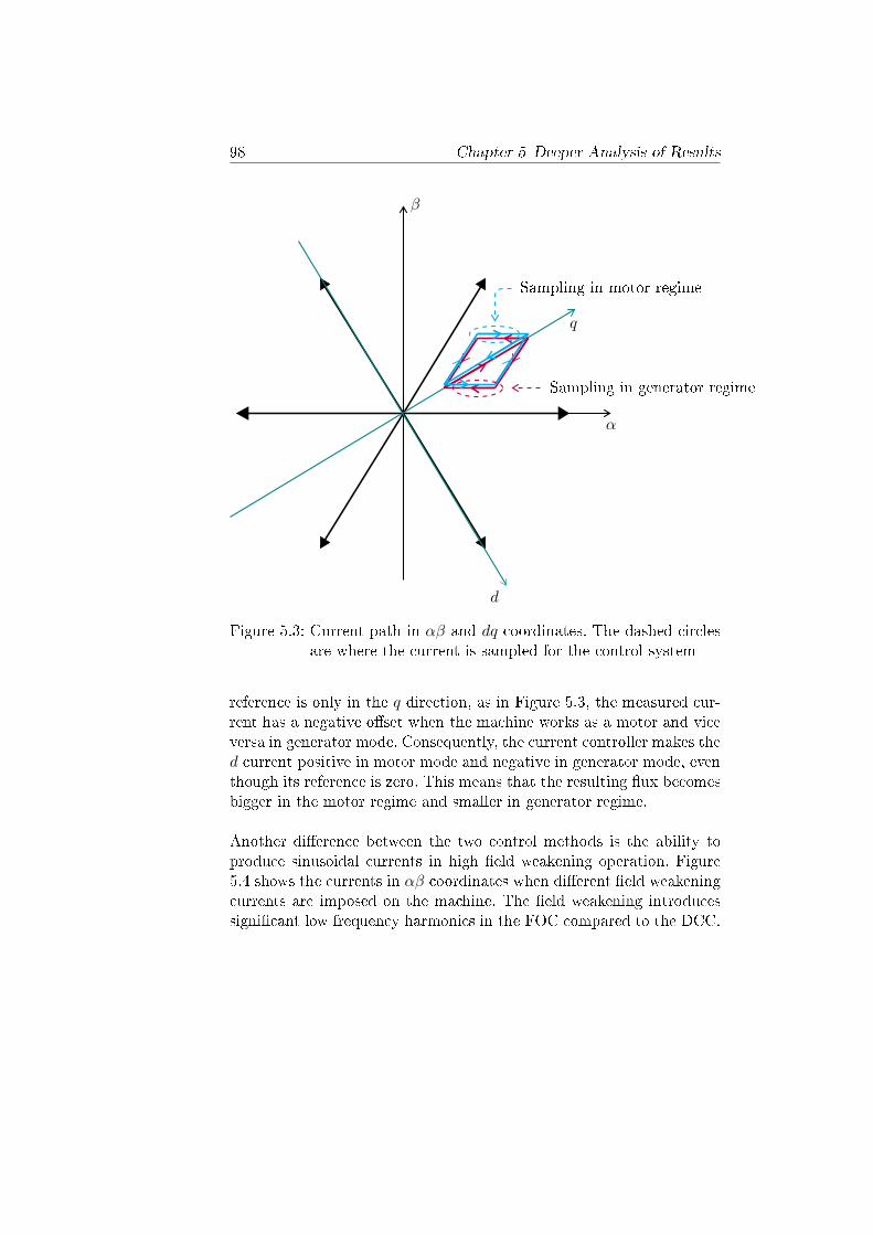
5.2 Field-oriented control signal path in the control system . 975.3 Current path in αβ and dq coordinates. The dashed cir-
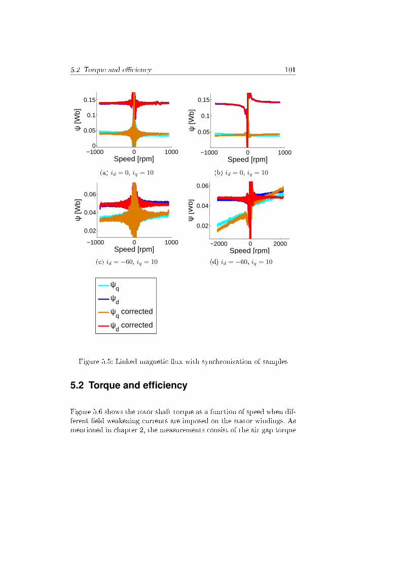
cles are where the current is sampled for the control system 985.4 αβ currents when dierent control methods are used . . 995.5 Linked magnetic ux with synchronization of samples . 1015.6 Torque with dierent eld weakening currents when iq =
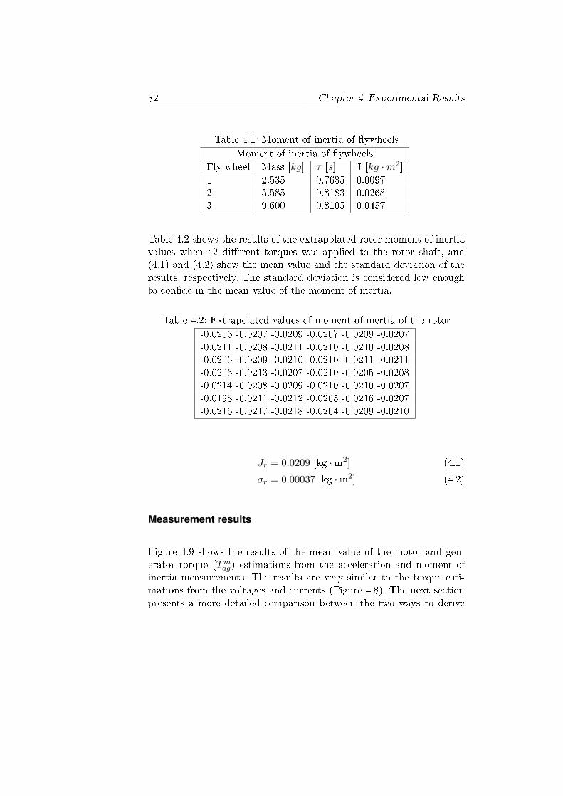
4.1 Moment of inertia of ywheels . . . . . . . . . . . . . . . 824.2 Extrapolated values of moment of inertia of the rotor . . 824.3 Absolute standard deviation of the torque derived from
measurements with four dierent moment of inertia onthe rotor shaft [Nm] . . . . . . . . . . . . . . . . . . . . 84
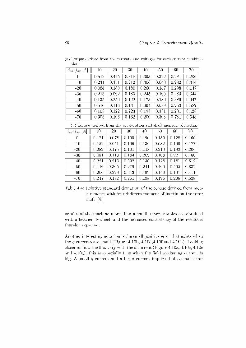
4.4 Relative standard deviation of the torque derived frommeasurements with four dierent moment of inertia onthe rotor shaft [%] . . . . . . . . . . . . . . . . . . . . . 86
4.1.1 The magnetic model . . . . . . . . . . . . . . . . 734.1.2 Comparison with results from FEMM simulations 744.1.3 Comparison with results from a constant speed
4.2 Torque derivation . . . . . . . . . . . . . . . . . . . . . . 804.2.1 From the ux and the currents (The air-gap torque) 804.2.2 From the acceleration and the moment of inertia
The dynamic testing method (DTM) project was created to assist theglobal endeavor to move away from the environmentally unfriendly andinsecure fossil-energy dependence. It took part in the bigger ventureELDRIVET, which intended to support the transition from combus-tion engines to electric drives in the Swedish vehicles eet. Within EL-DRIVET, the DTM project was assigned to develop a test method tofacilitate the development, manufacturing and employment of electri-cal machines in vehicles. Vehicle developers often consider permanentmagnets synchronous machines (PMSMs) for traction due to their highperformance; therefore, it was decided to focus on these machines.
This thesis presents the outcome of the DTM project. In hindsight, thedevelopment has been a success in the sense that the methodology showsa big potential to be useful for the industry. The quickness of the testprocedure and the need for little equipment and space makes it optimalfor fast characterizations of machines, which can be used as a rstfeed-back on machine designs or as a performance control for machinesin serial production. In addition, the method shows possibilities forincreased accuracy with more development. With all this in mind, thiswork can hopefully play a tiny part in saving the world.
2 Chapter 1 Introduction
1.1 Why dynamic testing?
The concept of testing machines dynamically is not new, and descriptionof such methods can be found in for instance the IEEE standard fortesting synchronous machines [1]. Here follows a general outline of theprocedures:
1. A drive accelerates a test object to a predened speed by imposingcurrents with constant amplitudes on the armature windings.
2. During the acceleration, a data acquisition system reads measure-ments of the acceleration of the rotor shaft.
3. The acceleration and moment of inertia of the shaft then yieldthe torque on the rotor as a function of the currents.
While these tests derive the torque characteristics of a machine, theDTM which this thesis presents extends the method to include magneticmodel characterization and eciency property measurements. This sub-section compares the DTM to other test methods and argues why thedevelopment of new procedures is relevant.
The rst part of the subsection discusses the magnetic model derivation.The magnetic model describes the currents relationship to the magneticux in the machine. Information about these properties give possibilitiesto design optimal control algorithms and gives valuable feedback tomachine designers. The results also make it possible to estimate theair-gap torque which can be compared to the rotor shaft torque forloss estimation in the machine. The second part discusses eciencytesting. Information about the eciency and losses is fundamental toperform lifetime estimations and life-cycle cost analysis on machines.Furthermore, the eciency together with the torque measurements givea direct indication if something is wrong with the machine.
1.1 Why dynamic testing? 3
Magnetic model derivation
The literature presents numerous ways to derive the electromagneticproperties of a PMSM. Dierent methods are used for dierent pur-poses: Simulations can optimize the performance of the machine in anearly design state. Supposing the material characteristics of the ma-chine are known, FEM simulations provide accurate information of amachine's characteristics [2], [3]. On-line methods verify machine pa-rameters while the machine is active in its application. Continuouslyupdated information can be used for sensorless control, diagnostics andmonitoring of the machine [4], [5], [6].
A third way to evaluate the machine is by o-line experimental tests.The o-line tests provide information for optimal control, machine diag-nostics and feed-back on prototype design. They can be divided up intotwo main categories: Stand-still methods (SSMs) and constant speedmethods (SCMs). As the name implies, the SSMs characterizes the ma-chine without motion; the rotor is locked mechanically while dierenttorque producing currents are imposed on the stator windings [7], [8],[9]. The reactions of the phase currents and voltages are then measured,and mathematical expressions derive the relationship between the cur-rent and magnetic ux linkage from the obtained data.
Stand-still methods have the drawback of not being able to provide in-formation about the ux linkage from the permanent magnets, and thetesting can not be extended to evaluate the eciency of the machine.Constant speed methods (CSM), on the other hand, can do both ofthese things. When the CSMs perform the testing, an additional brakemachine holds the speed of the test object constant while the clamp volt-ages are measured; the voltage measurements together with the PMSMsvoltage equations then yield the magnetic ux in post-processing calcu-lations. Even though the CSMs can derive all the necessary informationabout the machine, they require expensive equipment and test facilities.In addition, the time duration of the procedures is usually high, whichleads to bad time eciency and possible heating of the machine, whichin turn can lead to distortion in the measurement results.
4 Chapter 1 Introduction
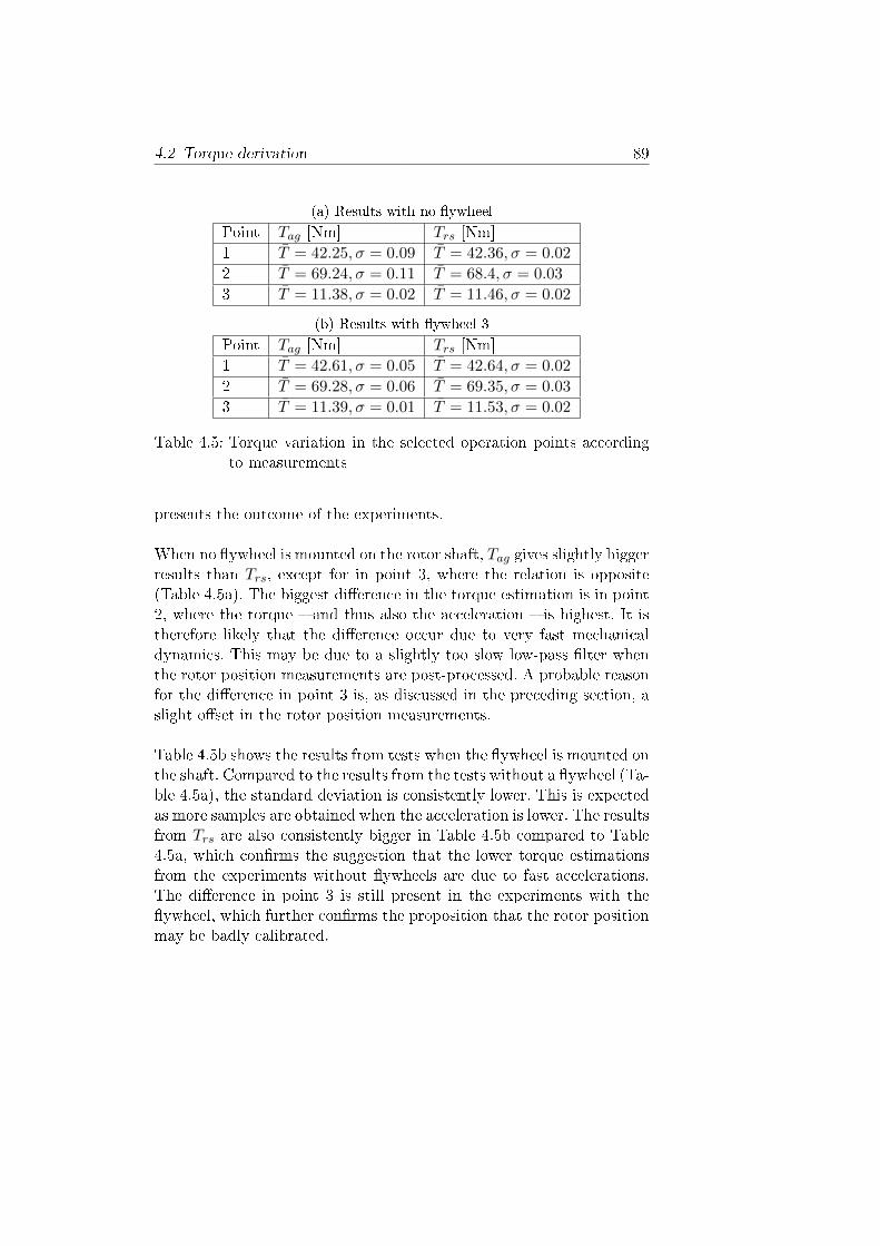
The drawbacks of the SSM and CSM characterization methods giveroom for alternative concepts, and one possible test alternative is theDTM. Even though torque producing currents are imposed on the testobject with an unlocked rotor, the test procedure does not involve abrake machine. Instead, the machine accelerates while the moment ofinertia of the rotor axis limits the acceleration. In the mean while,sensors and a data acquiring system obtain measurements which canderive the linked magnetic ux in post-processing calculations. Theo-retically, this methodology takes the best aspects of the SSM and theCSM concepts without losing anything. This, of course, requires thatthe accuracy of the results are not inferior to the other methods.
Efficiency testing
In contrast to electrically magnetized synchronous machines, asynchronousmachines and DC machines, there exists no standard (which the au-thor know of) which treats PMSMs. With that being said, there stillexist documents with guidelines for eciency testing of PMSMs, andthey generally base there recommendations on the standard for testingof synchronous machines [10], [11], [12], [1]. The synchronous machinestandard presents two ways to derive the eciency. In the rst method,the input and output power of the machine are measured. The eciencycan be calculated directly from the measurements as
η =output
input· 100 (1.1)
The second method requires that the dierent losses of the machineare measured rst, and the eciency may then be calculated accordingto
η = 100− losses · 100
input(1.2)
1.2 Objectives and Limits 5
for a motor, and
η = 100− losses · 100
losses+ output(1.3)
for a generator; this procedure is called the segregated losses method.
In most common ways to measure the eciency of a PMSM, an addi-tional test machine drives or brakes the test object throughout the testprocedures. A power meter measures the electric output power fromthe converter while rotor axis torque and speed measurements yield themechanical power of the machine. The eciency can then be calculatedwith the input-output method. If the test machine's loss characteristicsare known, speed-dependent losses may be measured from open circuittests at dierent frequencies. The resistance can be measured with animpedance meter and the eciency can then be derived by the segre-gated loss method. The changed temperature in the test object whichthe losses induce can also be measured throughout the tests. This re-quires special facilities with high control of the ambient temperature.
All of these methods demand time and require expensive equipment andfacilities. This motivates the development of new concepts for eciencyevaluation of machines. The dynamic test method introduces a methodwhich gives a quick and cheap estimation of the eciency and losses tocomplement to the the accurate but time and cost inecient constantspeed tests.
1.2 Objectives and Limits
The list below presents an overview of the objectives of this work:
• Extend the theoretical base of the method. Earlier articles fromthe division of Industrial Electrical Engineering and Automation
6 Chapter 1 Introduction
(IEA) of Lund University outline the concept [13]. This thesisshould give an in depth explanation of the theory behind it.
• Concentrate on the magnetic model derivation and torque char-acterization part of the DTM. The possibilities of eciency mea-surements and loss separation procedures should be discussed andevaluated as far as time and space allows.
• Present an extensive experimental evaluation of the method. Testresults should be compared to simulations and data from an es-tablished CSM. Discuss eventual deviations in the results.
• Present and discuss data acquisition procedures, post-processingof measurement data and the consequence of measurement errors.Present the methods that were used throughout the experimentaltests.
• Discuss strength and weaknesses of the method. Propose topicsfor future research.
Below follows the limits of the work:
• The measurement considerations part of chapter 2 focuses on themagnetic model identication part of the DTM (but a lot of in-formation there also applies to the eciency measurements andloss separation).
• The implications of measurement errors presented in chapter 2are not evaluated with either simulations or experimental tests.An analysis of that kind would indeed be interesting, but is outof the scope of this thesis.
• The loss separation possibility is only partly discussed in thisthesis, but is a good topic for future research.
• The theories about why unexpected measurement phenomena oc-cur that chapter 5 presents are not tested by simulations or ex-
1.3 Disposition 7
perimental tests. Such tests would contribute a lot to the thesis,but due to lack of time they were not performed.
1.3 Disposition
The list below gives the reader a quick introduction to the followingchapters in this thesis
• Chapter 2 (Theory and Method Description) gives a thorough ex-planation of the theory behind the dierent parts of the DTM. Itgoes through the testing process step by step and points out im-portant considerations along the way. Furthermore, current con-trol strategies which suit the DTM well are presented. The endof the chapter discusses data acquisition considerations, post-processing algorithms and consequences of measurement errors.
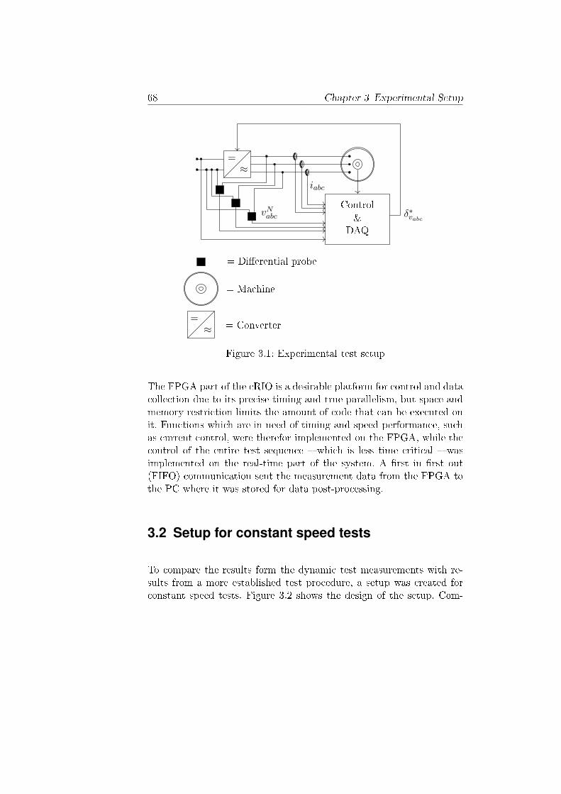
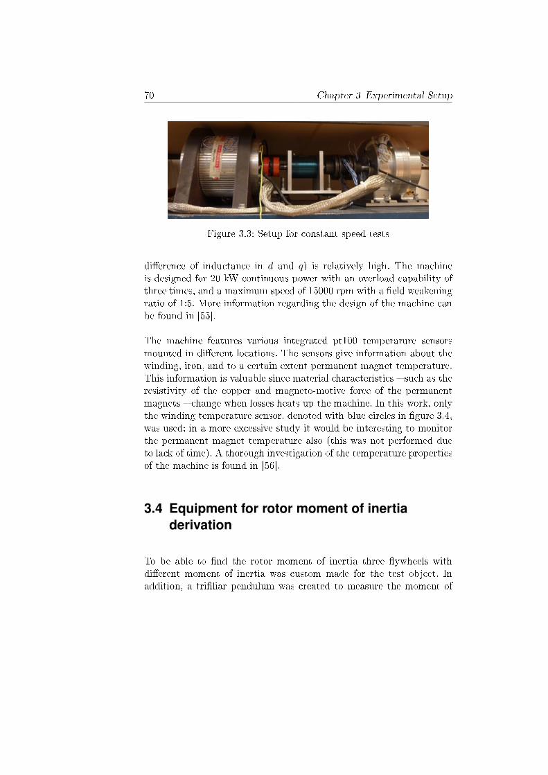
• Chapter 3 (Experimental Setup) describes the equipment thatwas used during the experimental tests. The test object as wellas the data acquisition and control system are taken into accountfor. Furthermore, the chapter describes the additional test benchwhich the constant speed tests used.
• Chapter 4 (Experimental Results) presents the results from DTMexperimental tests. The DTM is compared to a CSM in the mag-netic model identication section. The section also evaluates thetemperature's inuence on the results. Later parts of the chap-ter present an extensive consistency analysis of the DTM torquecharacterization. The analysis extends to compare the derived air-gap and rotor-shaft torque. The last parts of the chapter presenteciency and power factor results.
• Chapter 5 (Deeper Analysis of Results) discusses unexpected re-sults from Chapter 4. The ux's and torque's speed dependenceis given special attention.
8 Chapter 1 Introduction
• Finally, the last chapter concludes the thesis with remarks, rec-ommendations and proposals for future work.
1.4 Contribution
The main contribution from this work is the extensive evaluation ofdynamic testing of PMSMs. It gives the reader an idea of when themethod is suitable to use, and under which conditions it is not optimal.Furthermore, it gives suggestions for future research which can help theprogress within the eld of machine testing and characterization.
1.5 Publications
Marquez-Fernandez, F.J. Hall, S. Alaküla, M., "Dynamic testing char-acterization of a HEV traction motor," in Electrical Machines (ICEM),2014 International Conference on , vol., no., pp.1569-1575, 2-5 Sept.2014
Hall, S. Loayza, Y. Reinap, A. Alaküla, M., "Consistency analysis oftorque measurements performed on a PMSM using dynamic testing,"in Electrical Machines (ICEM), 2014 International Conference on, vol.,no., pp.1529-1535, 2-5 Sept. 2014
Hall, S. Loayza, Y., "An evaluation of two Direct Current Controlmethods implemented with LabVIEW on a FPGA," in Electrical Ma-chines and Systems (ICEMS), 2013 International Conference on, vol.,no., pp.1455-1460, 26-29 Oct. 2013
Reinap, A. Alaküla, M. Hall, S. Estenlund, S., "Performance estima-tion of hybrid excited machine with alternating pole conguration," inElectrical Machines (ICEM), 2014 International Conference on, vol.,no., pp.2638-2643, 2-5 Sept. 2014
Chapter 2
Theory & Method Description
This chapter presents a theoretical overview of the dynamic test method(DTM) together with measurement procedures, data post-processingapproaches, and consequences of measurement errors. The permanentmagnet synchronous machine (PMSM) model which works as the foun-dation for the theory of the derivation of magnetic model is adressedin the rst part of the chapter (section 2.1). The section explains theprocess of representing a PMSM in the rotating reference frame (dqframe), and presents a PMSM equivalent circuit in the dq frame.
Section 2.2 presents the DTM magnetic model identication process.The passage goes through the procedure of the experimental testing,and explains the theory behind how the magnetic ux is obtained fromthe measurements. Section 2.3.2 explains the DTM torque characteristicdetermination. The part only describes the theory of the data treatmentsince the post-processing system derives the torque from the same datathat is used in the magnet model identication. The DTM machineeciency derivation is addressed in section 2.4. The section presents thetheory of the calculations from the measurements and explains why themeasurements from the magnetic model derivation can not be reused.The section also discusses the possibility of expanding the DTM toinclude loss separation.
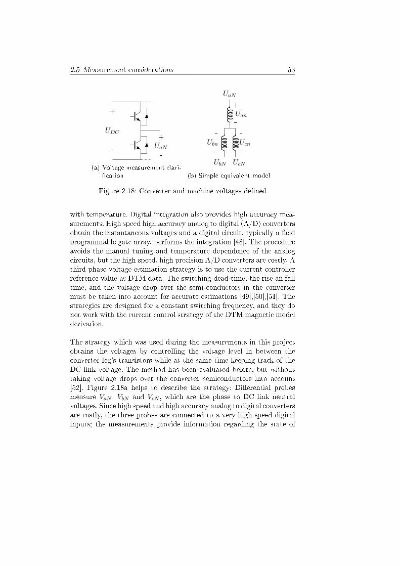
The data acquisition process is discussed in the last part of the chap-ter (section 2.5). The section addresses dierent methods to obtain thenecessary DTM data, and the methods that were used to derive the re-
10 Chapter 2 Theory & Method Description
sults which chapter 4 presents are explained. The passage also providesmeasurement data post-processing techniques and discusses the resultsof dierent measurement errors.
2.1 Machine model
To understand the theory behind the derivation of the PMSM magneticmodel, an analytical representation of the PMSM which shows the mag-netic ux relationship with the stator voltages and currents is necessary.The literature presents numerous variations of analytical PMSM mod-els with varying complexity. In addition to the standard components the stator winding resistance and inductance, and the induced voltage models can include iron losses modeled as a parallel resistance [14],a series resistance [15] or as a series voltage source [16]. Furthermore,phenomena such as inductance cross-coupling and cogging torque canbe taken into account [17], [18].
The models are often expressed in the dq frame, which represents theoscillating three phase system as constant values in a steady-state sit-uation, as proportional integrator (PI) current controllers usually needconstant steady-state reference values to perform well. The dq framealso suits the DTM magnetic model as optimal eld-weakening PI con-trol generally needs information about the ux characteristics of themachine. The following sections dene the dq frame and present thisworks PMSM equivalent model.
2.1.1 The dq frame
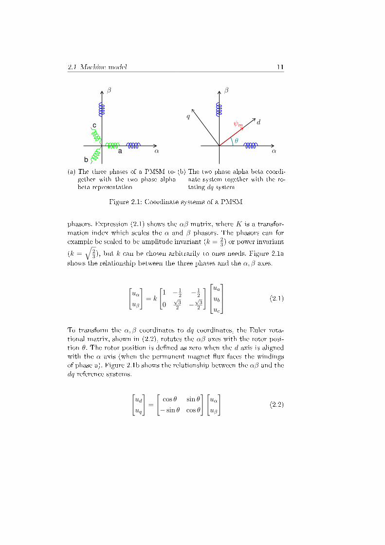
The dq frame is in this thesis dened as a coordinate system whichrotates counter clockwise with the electrical frequency, and where thed axis is aligned with the linked magnetic ux from the permanentmagnets. To derive the stator voltages and currents in the dq frame,the αβ matrix rst transforms the three phase phasors to two ortigonal
2.1 Machine model 11
α
β
ab
c
(a) The three phases of a PMSM to-gether with the two phase alphabeta representation
ψm
α
β
dq
θ
(b) The two phase alpha beta coordi-nate system together with the ro-tating dq system
Figure 2.1: Coordinate systems of a PMSM
phasors. Expression (2.1) shows the αβ matrix, where K is a transfor-mation index which scales the α and β phasors. The phasors can forexample be scaled to be amplitude invariant (k = 2
3) or power invariant
(k =√
23), but k can be chosen arbitrarily to ones needs. Figure 2.1a
shows the relationship between the three phases and the α, β axes.
[uα
uβ
]= k
[1 −1
2 −12
0√32 −
√32
]uaubuc
(2.1)
To transform the α, β coordinates to dq coordinates, the Euler rota-tional matrix, shown in (2.2), rotates the αβ axes with the rotor posi-tion θ. The rotor position is dened as zero when the d axis is alignedwith the α axis (when the permanent magnet ux faces the windingsof phase a). Figure 2.1b shows the relationship between the αβ and thedq reference systems.
[ud
uq
]=
[cos θ sin θ
− sin θ cos θ
][uα
uβ
](2.2)
12 Chapter 2 Theory & Method Description
+− ωψ
(iψd ,i
ψq
)q
−
+
ud
Rsdψ
(iψd ,iψq )
ddt isd
Rf
ifd
iψd
+−
ωψ
(iψd ,i
ψq
)d
−
+
uq
Rsdψ
(iψd ,iψq )
q
dt isq
Rf
ifq
iψq
Figure 2.2: Equivalent circuit of the PMSM in the dq reference frame
2.1.2 Equivalent circuit
Figure 2.2 shows the equivalent PMSM model of this work. The resis-tance Rs represents the voltage drop over the stator winding resistance;
dψ(iψd ,iψq )
dt the voltage drop due to change in the linked magnetic ux indq coordinates; the parallel resistance Rf the eddy current iron lossesin the machine; and the voltage sources represent the induced voltagedue to the linked magnetic ux. The iron losses are hard to model dueto their nonlinear behavior, and the resistance is mainly included fora conceptual purpose. As is seen in Figure 2.2, part of the measuredstator current is excites the eddy current losses, which means that notall of the stator current introduces ux linkage. Other phenomena, suchas hysteresis losses and excess iron losses also aect the linkage of themagnetic ux, but are left out of the model due to their complexity.The Kircho voltage law gives the voltage equations of the equivalentcircuit
2.2 Magnetic model identication 13
ud = Rsid +dψ
(iψd ,i
ψq
)d
dt− ωψ
(iψd ,i
ψq
)q (2.3)
uq = Rsiq +dψ
(iψd ,i
ψq
)q
dt+ ωψ
(iψd ,i
ψq
)d (2.4)
In the DTM, the control system holds the dq currents constant duringone test cycle. The derivative of the dq ux is therefore approximately
zero, and dψ(iψd ,iψq )
dt becomes zero (The iron losses make the ux linkagechange slightly with increased speed, but considering electrical dynam-ics the change is negligible). The voltage equations which are relevantfor the DTM become
ud = Rsid − ωψ(iψd ,i
ψq
)q (2.5)
uq = Rsiq + ωψ
(iψd ,i
ψq
)d (2.6)
2.2 Magnetic model identification
2.2.1 Test procedure
To test a PMSM with the DTM, the test object should be mountedrmly on a stable platform. A y-wheel is preferably mounted on themachine's rotor axis to slow down the mechanical dynamics when torqueis applied. The machine is connected to a variable frequency drive sys-tem which supplies the machine with voltage and current. For eachcurrent combination in the dq frame which is desirable to evaluate, atest cycle is performed:
14 Chapter 2 Theory & Method Description
Figure 2.3: Dynamic test sequence for magnetic model derivation
1. A voltage source drive accelerates the machine with a combinationof dq currents to a pre-dened negative speed.
2. The drive brakes the machine to stand-still with the same d cur-rent and the inverse of the q current from point 1).
3. Maintaining the same current combination, the drive acceleratesthe machine to the same magnitude of the speed as in point 1(but with a positive sign).
4. The drive brakes the machine to stand-still.
Notice that the machine works as a generator when it brakes, and thedrive system must therefor be able to absorb as well as deliver electricalenergy throughout the test sequence. A diode rectier bridge is therefornot suitable for the DTM test setup.
2.2 Magnetic model identication 15
Throughout the sequence, a data acquiring system (DAQ system) to-gether with sensors obtain voltage, current and rotor position measure-ment data. The obtained data from point 2) and 3), together with apost-processing system, derive information about the relationship be-tween the stator currents and the linked magnetic ux. Figure 2.3 showsan example of a test sequence where measurements from the part withinthe yellow rectangle are used to derive the linked ux.
2.2.2 Current control
A prerequisite for the dynamic test method to work is a current con-troller that keeps the current to its reference value, even when the in-duced voltages in the stator windings change very fast. In addition, thecontroller must perform without knowledge of the magnetic model ofthe machine. To handle this problem, a direct current control (DCC)scheme - a design which keeps the current within hysteresis limits bypicking a voltage vector which imposes a suitable current derivative -is used.
The DCC designs are known for being robust and to have fast tran-sient current response. The hysteresis limits of the controllers may beimplemented directly on the three phases, in the αβ frame or in the dqframe [19], [20], [21], [22]. Traditionally, the schemes have been designedfor analog electronics since the reaction time in choosing voltage vectorneeds to be very fast, but the development of high speed AD convertersand logic circuit technology has made high performance digital designseasier to implement [23], [24].
This section presents a scheme which suits the DTM test procedurewell. It was created for a eld programmable gate array (FPGA), whichwas used as the core of the experimental testing control system setupthroughout this project. Hopefully the section gives the reader ideas ofhow a suitable DTM current control algorithm can look like, even if theFPGA technology is not available.
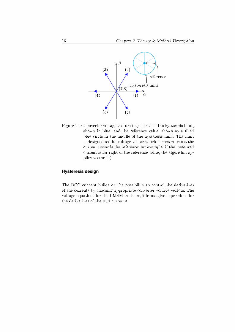
16 Chapter 2 Theory & Method Description
α
β
(1)(4)
(2)(3)
(5) (6)
(7,8)hysteresis limit
reference
Figure 2.4: Converter voltage vectors together with the hysteresis limit,shown in blue, and the reference value, shown as a lledblue circle in the middle of the hysteresis limit. The limitis designed so the voltage vector which is chosen tracks thecurrent towards the reference; for example, if the measuredcurrent is far right of the reference value, the algorithm ap-plies vector (4)
Hysteresis design
The DCC concept builds on the possibility to control the derivativesof the currents by choosing appropriate converter voltage vectors. Thevoltage equations for the PMSM in the α, β frame give expressions forthe derivatives of the α, β currents
2.2 Magnetic model identication 17
uα = Rsiα + Ldiαdt− ω (Liβ + ψm sin θ) (2.7)
uβ = Rsiβ + Ldiβdt
+ ω (Liα + ψm cos θ) (2.8)
→diαdt
=uα + ω (Liβ + ψm sin θ)−Rsiα
L(2.9)
diβdt
=uβ − ω (Liα + ψm cos θ)−Rsiβ
L(2.10)
The expressions above show that depending on which voltage vectorthat the control algorithm chooses to use, the currents can be controlledto track in a certain direction in the α, β frame. If the current deviatesfrom the reference value, some of the voltage vectors move the currentin the wanted direction. The DCC algorithm can therefore be designedto pick the best vector possible as soon as the current error is so bigthat the current tracks outside of the hysteresis limit.
Figure 2.4 shows the hysteresis limit that dictates when the controlsystem reevaluates which voltage vector it applies. The limit is circularto make the error as uniformly distributed as possible. The controlsystem picks vector depending on the angle of the error in regard tothe α axis. Once the current tracks outside of the circle, the algorithmchooses a new vector to decrease the error. The controller keeps thesame vector until the current tracks outside of the limit once again,whereupon the choice of vector is reevaluated.
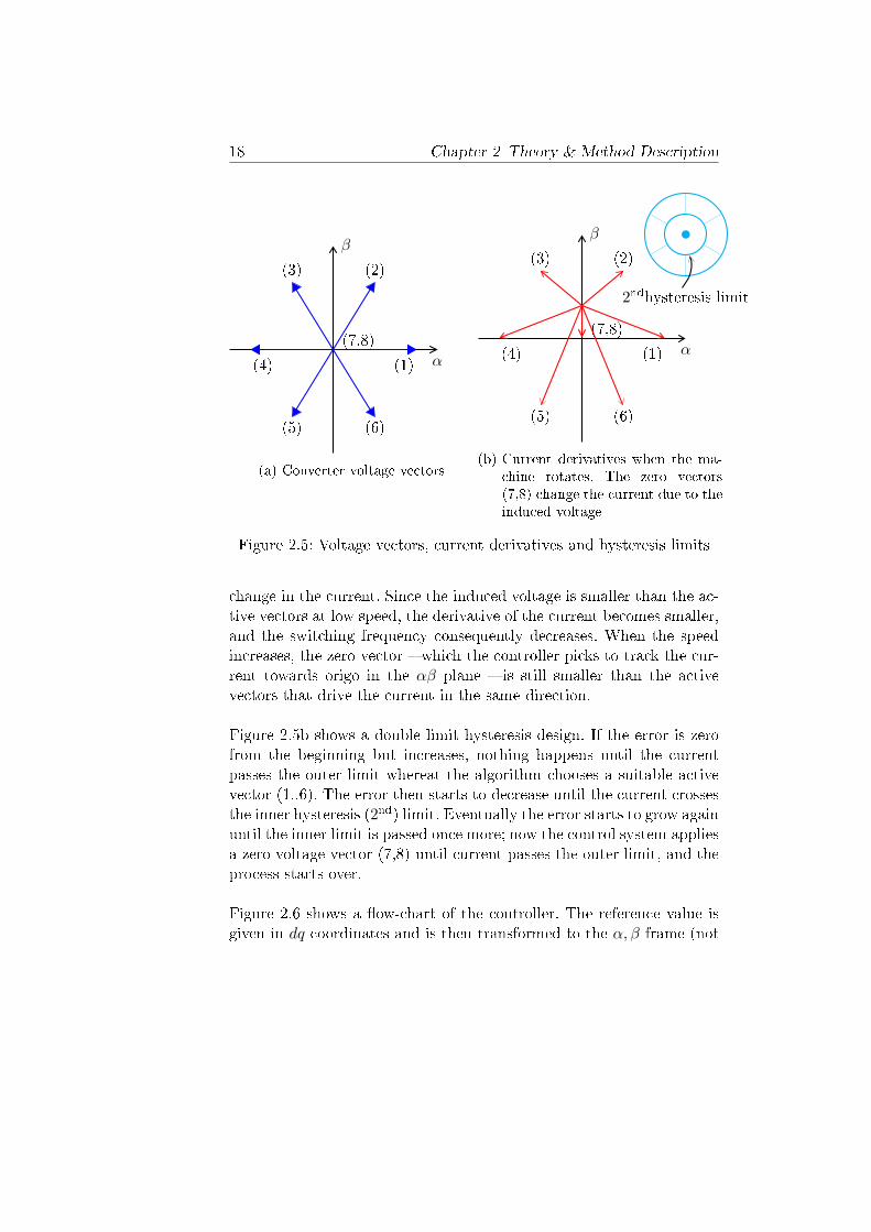
Utilizing the zero vector
In contrast to a PWM modulated control, the DCC introduces a vari-able converter switching frequency. This can become problematic ashigh current derivatives lead to a high switching frequency. A way toimprove the design in this aspect is to introduce a second hysteresis limitwhich decides when to chose the zero vector. The zero vector does notapply any voltage from the converter on the phase windings. Instead,the induced voltage from the induction in the stator windings creates a
18 Chapter 2 Theory & Method Description
α
β
(1)(4)
(2)(3)
(5) (6)
(7,8)
(a) Converter voltage vectors
α
β
(1)(4)
(2)(3)
(5) (6)
(7,8)
2ndhysteresis limit
(b) Current derivatives when the ma-chine rotates. The zero vectors(7,8) change the current due to theinduced voltage
Figure 2.5: Voltage vectors, current derivatives and hysteresis limits
change in the current. Since the induced voltage is smaller than the ac-tive vectors at low speed, the derivative of the current becomes smaller,and the switching frequency consequently decreases. When the speedincreases, the zero vector which the controller picks to track the cur-rent towards origo in the αβ plane is still smaller than the activevectors that drive the current in the same direction.
Figure 2.5b shows a double limit hysteresis design. If the error is zerofrom the beginning but increases, nothing happens until the currentpasses the outer limit whereat the algorithm chooses a suitable activevector (1..6). The error then starts to decrease until the current crossesthe inner hysteresis (2nd) limit. Eventually the error starts to grow againuntil the inner limit is passed once more; now the control system appliesa zero voltage vector (7,8) until current passes the outer limit, and theprocess starts over.
Figure 2.6 shows a ow-chart of the controller. The reference value isgiven in dq coordinates and is then transformed to the α, β frame (not
2.2 Magnetic model identication 19
+ x, y → r, φ G(s)i∗α,β
-
iα,β
Figure 2.6: Flowchart of the direct current control in αβ coordinates.The box after the subtraction represents a transformationfrom Cartesian to polar coordinates
shown in the gure). This becomes the reference input to the algo-rithm. The error in α, β Cartesian coordinates is transformed to polarcoordinates, and the resulting angle and magnitude are fed into thestate-machine which decides which vector that should be chosen for thenext time instant.
EMF compensation
Since the induced voltage drags the current towards origo in the αβframe, the inner hysteresis limit gives rise to a current error. Further-more, an increased speed tend to worsen this error since the activevectors lose the capability to drive the current away from origo. Figure2.5b which shows the resulting current derivatives for each convertervoltage vector explains the phenomenon. In the gure, the machinerotates, and the resulting emf drives the current towards origo when thecontrol system chooses a zero vector (7,8). If the current hits the lowerpart of the outer hysteresis limit, the algorithm picks vector 2 or 3 todrive the current away from origo. Since the zero vector current deriva-tive aects the direction of the active vector current derivatives, vector2 and 3 drive the current to the side of the hysteresis limits rather thanthe top. Therefore, the current get stuck in the lower part of the twohysteresis circles. This introduces an error in regard to the reference. Inαβ, the error is varying with the rotor position, but the magnitude ofthe error is approximately proportional to speed. Therefore, the averageerror in dq coordinates is independent of rotor position but aected by
20 Chapter 2 Theory & Method Description
+ CC
MAF
+ ci ·∑
dqαβ
αβdq
-
i∗d,q id,q
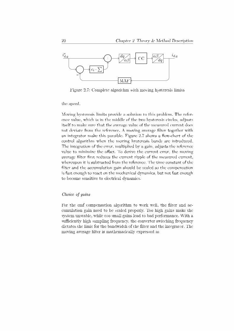
Figure 2.7: Complete algorithm with moving hysteresis limits
the speed.
Moving hysteresis limits provide a solution to this problem. The refer-ence value, which is in the middle of the two hysteresis circles, adjustsitself to make sure that the average value of the measured current doesnot deviate from the reference. A moving average lter together withan integrator make this possible. Figure 2.7 shows a ow-chart of thecontrol algorithm when the moving hysteresis bands are introduced.The integration of the error, multiplied by a gain, adjusts the referencevalue to minimize the oset. To derive the current error, the movingaverage lter rst reduces the current ripple of the measured current,whereupon it is subtracted from the reference. The time constant of thelter and the accumulation gain should be scaled so the compensationis fast enough to react on the mechanical dynamics, but not fast enoughto become sensitive to electrical dynamics.
Choice of gains
For the emf compensation algorithm to work well, the lter and ac-cumulation gain need to be scaled properly. Too high gains make thesystem unstable, while too small gains lead to bad performance. With asuciently high sampling frequency, the converter switching frequencydictates the limit for the bandwidth of the lter and the integrator. Themoving average lter is mathematically expressed as
2.2 Magnetic model identication 21
h(n) =1
N
N−1∑k=0
δ[n− k] (2.11)
where N is equal to the number of elements. Written in frequency do-main, the transfer function becomes
H(ω) =1
N
∑e−jωn (2.12)
which with Euler identity may be rewritten as
H(ω) =1
N
∣∣∣∣sinwn2sinw2
∣∣∣∣ (2.13)
where ω is equal to the cut-o frequency divided by the sampling fre-quency times two pi. The cut-o frequency is when H(ω) = 1√
2, and
the N which satises (2.13) is the number of elements used in the lter.Simulations show that
ωb =ωsw10
(2.14)
where ωsw is the converter switching frequency is a suitable cut-ofrequency for the lter. The integral gain is then chosen as 10 timessmaller than 1
N
ci =1
10 ·N(2.15)
2.2.3 Deriving the linked flux
Once the measurement data is acquired, the linked magnetic ux isderived from the measured voltages, the measured currents and the
22 Chapter 2 Theory & Method Description
rotor position. A rewrite of (2.5) and (2.6) yields expressions for theux
ψ
(iψd ,i
ψq
)q =
ud −Rsisdω
(2.16)
ψ
(iψd ,i
ψq
)d =
−uq −Rsisqω
(2.17)
The equivalent circuit of the machine (Fig. 2.2) shows that the ironlosses inuence the linked ux dierently if the machine works as agenerator or as a motor. If the currents are held constant, the inducedvoltages change sign depending on the working regime. This means thatthe currents that ow through the equivalent eddy current resistanceschange sign.
Even if the sign of the induced voltages vary, the magnitudes of them and the size of the eddy current resistance are approximately the samewhen the magnitude of the electric frequencies are equal, regardless ifthe machine works as a generator or as a motor. As a consequence,the magnitude of the eddy current loss currents are also approximatelyequal under the same conditions, and hence follows
isd ≈iψd,motor + iψd,generator
2(2.18)
isq ≈iψq,motor + iψq,generator
2(2.19)
for each electrical frequency. Supposing that the ux which is generatedfrom iψmotor and i
ψgenerator has a linear relationship to the currents, (2.18)
and (2.19) can be directly translated to expressions for the ux
2.2 Magnetic model identication 23
ψ(isd,i
sq)
d ≈ψ
(iψd ,i
ψq
)d,motor + ψ
(iψd ,i
ψq
)d,generator
2(2.20)
ψ(isd,i
sq)
q ≈ψ
(iψd ,i
ψq
)q,motor + ψ
(iψd ,i
ψq
)q,generator
2(2.21)
Combining (2.16) and (2.17) together with (2.20) and (2.21), expres-sions for the ux using measurements from both when the machine isaccelerating and when it is braking are reached
ψ(isd,i
sq)
q ≈uωd−Rsi
sd
ω +u−ωd −Rsi
sd
−ω2
=uωd − u
−ωd
2ω(2.22)
ψ(isd,i
sq)
d ≈−uωq−Rsisq
ω +−u−ωq −Rsisq
−ω2
=−uωq + u−ωq
2ω(2.23)
Deriving the ux in this way has some noteworthy implications:
1. The equations yield the average value of the ux when the ma-chine works as a generator and a motor, for the same stator wind-ing currents.
2. Information about the stator winding resistive voltage drop is notneeded for calculations of the linked ux. This is true only if thetemperature rise in the windings is insignicant during one testcycle.
3. The linked ux is constant over the whole frequency range. Thismakes it possible to use a lot of measurements during one speedsequence, which can be averaged for a better result.
Figure 2.8 shows an example of the d ux linkage results for a typicaltest sequence. The red line is the rst term of the numerator on the
24 Chapter 2 Theory & Method Description
100 200 300 400 500
0.1
0.15
0.2
Speed [rpm]
ud−ω/−ω
udω/ω
(udω+u
d−ω)/2ω
Figure 2.8: Flux derivation using the dynamic test method. The redline is the rst term in the denominator of the right handside in (2.22), the blue line is second, and the green is theresult from the total expression
right hand side of (2.22), which represents the accelerating part of thesequence (where the machine works as motor). The blue line is thesecond term, which represent the braking part. The green line is themean value of the two which is the total results of the right hand sideof (2.22). As the results become unstable when approaching zero speed,it is recommended that measurements when the speed is low are notused for the derivation of the ux.
2.3 Torque derivation
2.3.1 Air-gap torque
In addition to linked magnetic ux maps, the dynamic test methodprovides the torque characteristics of the test object. The ux for aspecic current combination together with the currents yield the air-
2.3 Torque derivation 25
gap torque in between the rotor and the stator. The equation for theair-gap torgue can be deduced from the electric power
Pe = uaia + ubib + ubib (2.24)
Transforming the voltage and current with the power-invariant trans-
form (K =√
23), (2.24) together with (2.1) and (2.2) yield
Pe = udisd + uqi
sq (2.25)
Removing the copper losses in the stator windings, which do not con-tribute to any torque, (2.25) with (2.5) and (2.6) become
Pe = ω(−ψ(iψd ,i
ψq
)q isd + ψ
(iψd ,i
ψq
)d isq) (2.26)
Power can also be expressed as force times speed, or in this case, thetorque times the frequency
Pe = Tagω (2.27)
Combining (2.26) with (2.27), a nal expression for the electromagnetictorque in the air-gap is reached
Tag = ψ
(iψd ,i
ψq
)d isq − ψ
(iψd ,i
ψq
)q isd (2.28)
Using the derived ux from the DTM, the mean torque for the motorand the generator operation for every current combination in the dqframe is derived by
26 Chapter 2 Theory & Method Description
Tmag = ψ(isd,i
sq)
d isq − ψ(isd,i
sq)
q isd (2.29)
2.3.2 Rotor shaft torque
Newton's second law gives a relationship between the acceleration of anobject with a specic mass when it is exposed to a force
F = ma (2.30)
If an additional force in the opposite direction of the rst aects thesystem, the equation can be extended to
F = ma+ Fext (2.31)
where Fext is the additional force that is imposed on the object. Con-sidering a cylinder as the rotor in a PMSM (2.31) can be translatedto
Trs = Jdωmdt
+ Text (2.32)
where Trs is the rotor shaft torque, which is the resulting tangentialradial force that acts on the rotor shaft times the radius of the rotor(the force that makes the cylinder rotate around it's central axis); J
is the rotor shaft moment of inertia; dωmdt represents the acceleration ofthe mechanical frequency of the rotor; and Text is an external torqueon the rotor. In a PMSM, the rotor shaft torque can be divided up intotwo main components: the air-gap torque Tag, and the mechanical losstorque Tloss.
2.3 Torque derivation 27
Tag − Tmecloss = Jdωmdt
+ Text (2.33)
The external torque is a load when the machine works as a motor,and a driving torque when the machine works as a generator. In theDTM, neither a drive nor a load is connected to the rotor shaft, andconsequently Text is zero. The loss torque brakes the machine in themotor regime, which means that the air-gap torque and the loss torquehave dierent signs. In the generator regime on the other hand, the losstorque has the same sign as the air-gap torque. This means that if themagnitude of the loss torque is considered independent of the rotationaldirection, it is canceled if the calculation uses measurements from boththe motor and the generator operation, as long as the frequency andthe air-gap torque, which means dq currents, are the same. The air-gaptorque for one dq current combination becomes
Tmag = Jdωm,motor
dt +dωm,generator
dt
2(2.34)
Figure 2.9 shows an example of how the mean torque over a speed se-quence is derived. When the machine works as a generator (blue line)the torque is higher since the loss torque has the same sign as the elec-tromagnetic torque. When the speed increases, the torque increases aswell as the iron losses and the mechanical losses are speed dependent.On the other hand, when the machine works as a motor (red line), theloss torque works against the acceleration, and the resulting torque be-comes lower. The green line is the mean value of the two cases, and isindependent of speed. When the speed approaches zero, the results os-cillates, and it is recommended to not include low speed measurementsin the torque derivation.
28 Chapter 2 Theory & Method Description
0 200 400 60011
12
13
14
15
Speed [rpm]
Tor
que
[Nm
]
Figure 2.9: Mechanical torque derivation using the dynamic testmethod. The blue line is when the machine works as gener-ator, the red line when it works as a motor, and the greenline is a mean value between the two
Derivation of moment of inertia
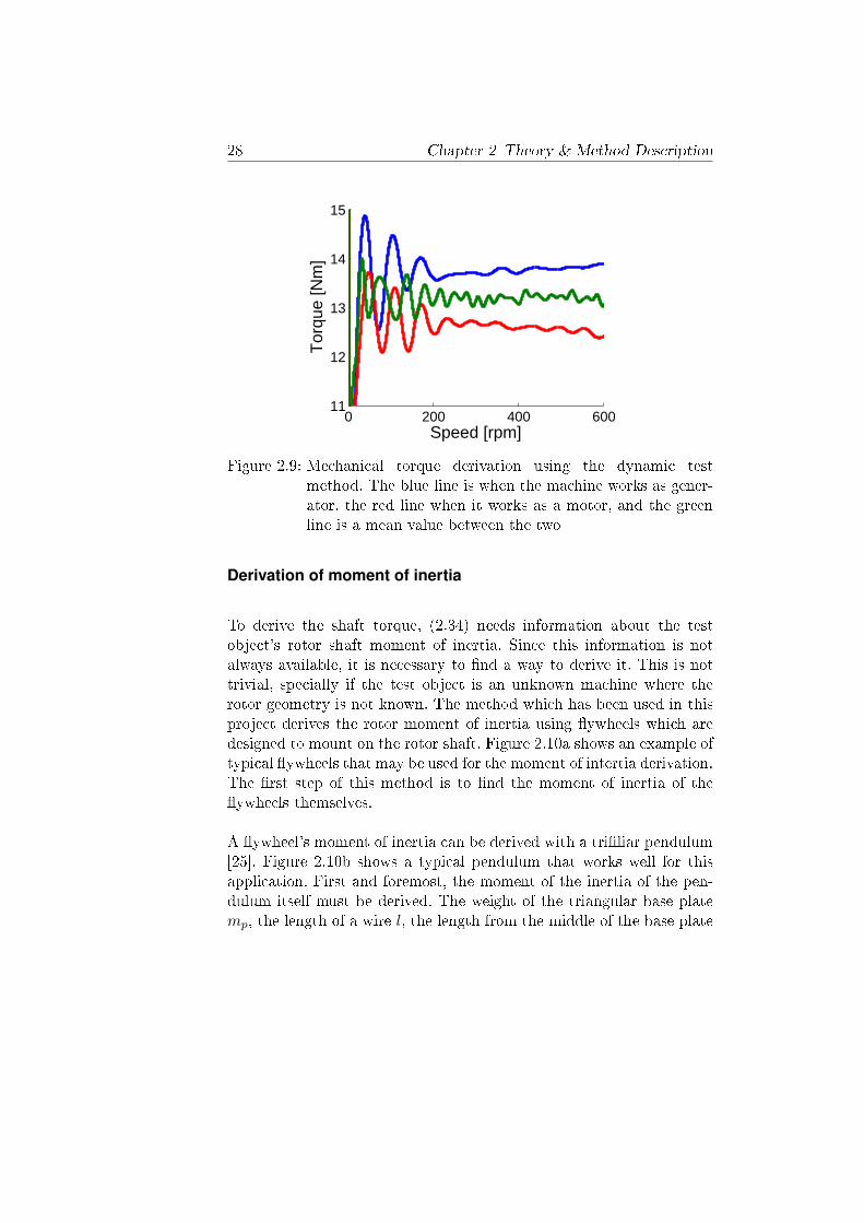
To derive the shaft torque, (2.34) needs information about the testobject's rotor shaft moment of inertia. Since this information is notalways available, it is necessary to nd a way to derive it. This is nottrivial, specially if the test object is an unknown machine where therotor geometry is not known. The method which has been used in thisproject derives the rotor moment of inertia using ywheels which aredesigned to mount on the rotor shaft. Figure 2.10a shows an example oftypical ywheels that may be used for the moment of intertia derivation.The rst step of this method is to nd the moment of inertia of theywheels themselves.
A ywheel's moment of inertia can be derived with a triliar pendulum[25]. Figure 2.10b shows a typical pendulum that works well for thisapplication. First and foremost, the moment of the inertia of the pen-dulum itself must be derived. The weight of the triangular base platemp, the length of a wire l, the length from the middle of the base plate
2.3 Torque derivation 29
(a) Flywheels (b) Triliar pendulum
Figure 2.10: Typical ywheels and a pendulum which can be used toderive the rotor moment of inertia
to a wire r, the gravity g, and the period time when the pendulum isset in motion τ determine the pendulums moment of inertia accordingto
Jp = mpr2τ2g
4πl(2.35)
Once Jp is known, the masses of the ywheels establish their momentof inertia as
Jf = (mp +mf )r2τ2g
4πl− Jp (2.36)
When the moment of inertia of the ywheels are known, an extrapola-tion of a series of accelerations with the dierent ywheels mounted on
30 Chapter 2 Theory & Method Description
0 0.005 0.01
−0.02
0
0.02
0.04
(dω/dt)−1 [(s/rad)2]
Mom
ent o
f ine
rtia
[kg
⋅m2 ]
(a) Moment of inertia extrapolationwith on torque
0 0.005 0.01
−0.02
0
0.02
0.04
(dω/dt)−1 [(s/rad)2]
Mom
ent o
f ine
rtia
[kg
⋅m2 ]
(b) Moment of inertia extrapolationwith several torques
Figure 2.11: Extrapolation of the rotor moment of inertia using threeywheels. One red line represents one specic torque, whilethe blue dots along the red lines are the dierent momentsof inertia
the rotor shaft ascertains the PMSM's rotor moment of inertia. Figure2.11a shows an example of the procedure. The red line is an interpo-lation of J as a function of the inverse of dω
dt when the same torqueaccelerates the machine with four dierent moment of inertia on therotor shaft (three cases with dierent ywheels mounted and one casewithout ywheel). The line also extends to extrapolate the rotor mo-ment of inertia, which is when (dω/dt)−1 is zero. Figure 2.11b showsthe rotor moment of inertia derivation when several dierent torquesare used. All extrapolations converge towards the same point; this isthe moment of inertia of the rotor.
When the moment of inertia estimations for a satisfying amount ofdierent torques on the rotor shaft are available, the mean value of theresults is calculated according to
y =1
n
n∑i=1
y(i) (2.37)
2.3 Torque derivation 31
To get a notion of how much the dierent inertia estimation dier, thestandard deviation of the result can be calculated according to
σ =
√√√√ 1
n− 1
n∑i=1
(y(i)− y)2 (2.38)
2.3.3 Conclusions
As the previous sections show, both the ux and current and the mo-ment of inertia and acceleration can derive the mean air-gap torque(Tmag). As a consequence, the moment of inertia can be derived directlyfrom the DTM measurements since
Jdωm,motor
dt +dωm,generator
dt
2= ψmd iq − ψmq id (2.39)
J =2(ψ
(isd,isq)
d iq − ψ(isd,i
sq)
q id)dωm,motor
dt +dωm,generator
dt
(2.40)
The moment of inertia derivation above makes it possible to obtainthe rotor shaft torque both for when the machine works as a motorand as a generator without the need of a pendulum and ywheels orknowledge about the rotor geometry. Consequently, the loss torque canbe quantied without a pendulum and ywheels or knowledge aboutthe rotor geometry.
With the straight forward way to derive the moment of inertia which(2.40) introduces, it may seam unnecessary to include the additionalmethod (presented in the previous section). The additional method isincluded due to uncertainty regarding accuracy. Chapter 4 presents aconsistency analysis to control whether the (2.40) can derive J accu-rately or not (section 4.2.3).
32 Chapter 2 Theory & Method Description
2.4 Efficiency tests
2.4.1 Test procedure
The DTM needs a second iteration of experimental tests to derive theeciency of the test object. There are two main reasons why the resultsfrom the rst test cycles described in subsection 2.2.1 can not bereused
1. The rst iteration of cycles does not test the machine at very highspeeds. Since the speed's limit is set manually to a value whichassures that the induced voltage does not reach the voltage limit,higher speeds are left out.
2. The current controller which is used in the magnetic model iden-tication works with a variable frequency (section 2.2.2 describesthe current controller), which makes it problematic to measurethe quasi-instantaneous voltage accurately. This is not a problemwhen the magnetic ux linkage is derived since many measure-ments can be average to derive an accurate result, but the e-ciency derivation demands accurate voltage measurements through-out the test sequence.
Finding the maximum speed
The rst challenge for the design of the new test sequence is thus tond the maximum possible speed for each testing point. The maximumspeed varies depending on the stator current. One approach to nd thespeed limit is to calculate an estimation of the maximum frequency from(2.5) and (2.6) (this demands that the stator resistance is estimatedbeforehand). The DTM magnetic model derivation provides the linkedmagnetic ux, and the DC link voltage of the drive denes the maximumvoltage. The modulus of the dq voltage phasor is expressed as
2.4 Eciency tests 33
|udq| =√u2d + u2q (2.41)
substitution of ud and uq with the expressions on the right hand sidesof (2.5) and (2.6) yield
|udq| =√
(Rsid − ωψq)2 + (Rsiq + ωψd)2 (2.42)
Assuming |udq| is the maximum voltage (|um|), the frequency is theonly unknown variable in (2.42). A rewrite of (2.42) yields a secondorder equation of ω with only one positive solution
The expression above derives the maximum speed for the fundamen-tal frequency of the induced voltage, but since the induced voltage al-ways carries harmonics, the calculations tend to overestimate the speedlimit. A scaling factor below one provides a safety margin, but since theharmonic content of the induced voltage diers depending on currentcombination, a suitable value of the scaling factor can be hard to nd.
A second method to derive the maximum speed controls if the referencevoltage value from the controller output reaches the maximum allowedvalue. This is a straight forward on-line method, and if the algorithmsets the limit as a function of the DC link voltage, it takes uctuationsin that voltage level into account. The reference depends heavily on thegains of the controller, and high P gains can lead to big ripples. As aconsequence, the algorithm tends to limit the speed at an unnecessarylow value. This can be taken into account for with a low-pass lter, butthe lter must not be slow to underestimate the induced voltage. If thebandwidth of the lter is known, the delay can be taken into accountfor by a set limit between the maximum allowed voltage and the ltered
34 Chapter 2 Theory & Method Description
reference value. The method can be further enhanced if the dead timeand the rise and fall times of the IGBTs are taken into account.
Another approach is to try to nd the speed limit experimentally this is the method the tests used throughout this project. Experimen-tal tests provide information about the maximum speed for a currentcombination when the controller no longer can keep the currents to theirreference. This is a dangerous way of investigating the maximum speedsince the eld weakening current must be maintained at high speeds.If the current controller fails to maintain id, the induced voltage mayrise above the drive's maximum available voltage, which can have se-vere consequences such as demolition of the drive's DC link capacitorbank.
A specially designed prioritization algorithm in the current controllersolves this problem: An observer constantly checks how much the aver-age value of the modulus of the dq current deviates from the reference.If the current deviates too much, the controller lowers the modulus andchanges the sign of the q current the smaller current makes sure thatthe voltage limit is not breached. The new current combination gener-ates a negative torque which brakes the machine until the rotor standsstill whereupon the controller sets the reference to zero. The point wherethe current starts to deviate gives the information about the maximumspeed. Since this point is on the very limit of the availible voltage, thelimit should be reduced with a constant value to make sure that thecontrol of the eld weakening current is not lost.
A current controller which is fast and robust is a necessity for thisalgorithm. Since the controller which is used in the magnetic modelidentication test procedure fullls these criteria, it can advantageouslybe reused for these tests.
Switching current controller
Despite the advantages of the DCC scheme, the variable switching fre-quency which the method gives rise to makes it to hard to measure
2.4 Eciency tests 35
+ kp + kis
+ +
jω ~ψsdq
(~isdq
)1
Rs+sL( ~isdq)
-
~is∗dq
-
~isdq
control system machine model
Figure 2.12: Flowchart of the eld oriented vector controller
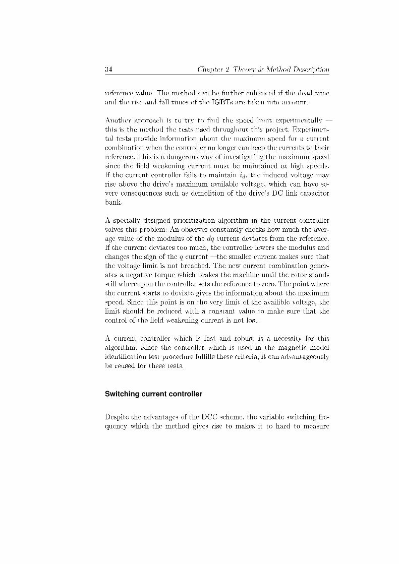
the converter voltages over small time windows accurately. Since theeciency measurements need good quasi-instantaneous voltage mea-surements, a well performing DTM needs an additional current controlmethod for the eciency testing.
The eld oriented PI current controller in the rotating coordinate sys-tem is a well established strategy for controlling currents in electri-cal machines [26]. The control system controls the drive's converterwith pulse width modulated signals which means that the switchingfrequency can be constant. Figure 2.12 shows a owchart of the con-troller applied on a non-linear PMSM. The machine is modeled in polarcoordinates instead of the Cartesian so one owchart is enough to de-scribe the system. The variable ~is is dened as
~isdq = | ~isdq|ejα
α = tan−1
iqid
| ~isdq| =√i2d + i2q
The denition leads to the voltage equation
~vsdq = Rs ~isdq + L( ~isdq)d ~isdqdt
+ jω ~ψsdq(~iψdq) (2.44)
36 Chapter 2 Theory & Method Description
where ~ψsdq is the total linked ux vector which includes both the per-manent magnet ux and the ux due to the stator currents. The equa-tion above describes the stator current's relationship with the drive'svoltage, which is controlled by the control system. Note that (2.44) ex-presses the derivative of the ux dψs
dt as an inductance times the deriva-tive of the current. This paraphrasing makes it possible to express themachine as a RL load, which is valuable when deciding the gains of thecontroller. A laplace transformation of the equation above yields theexpression for the load in the frequency domain
Isdq(s)
U sdq(s)− jωΨsdq(s)
=1
Rs + Ls(2.45)
Due to the non-linearity of the machine's ux linkage, the inductance and also to a certain extent the ux linkage of the permanent magnets is dependent on the stator current. Therefor, no load disturbance orpure feed-forward exist in this model (in most cases, these type of con-trols see the induced voltage due to the permanent magnet ux as a loaddisturbance which can be feed-forwarded without knowledge about thestator current). On the other hand, since the magnetic model deriva-tion provides ux maps as functions of the stator currents, informationabout the ux linkage and inductance can be obtained by look-up ta-bles. When the scheme in Figure 2.12 adds the induced voltage to theoutput signal of the control system, the PI controller only acts on thevoltage over the RL load; the removal of the induced voltage from thesystem means that it is no longer aected by the mechanical dynam-ics. Note that the look-up table approach in contrast to the moreconventional use of constant values for the inductance and the linkedpermanent magnet ux takes the magnetic non-linearity due to satu-ration in the core of the machine into account.
Choosing PI gains
As mentioned above, the PI controller only acts on the system as aRL load. With this in mind, the proportional and integral gain can bedetermined so that only one pole exists in the whole closed loop system.
2.4 Eciency tests 37
The internal model control (IMC) method provides the necessary stepsto obtain the gains with the possibility to chose the bandwidth of thesystem[27].
As the control scheme removes the induced voltage from the closed loopsystem, the open loop transfer function of the machine model becomes
G(s) =1
Rs + sL(2.46)
On the control system side, the open loop transfer function becomes
F (s) = kp +kis
(2.47)
The complete closed loop transfer function of the system is formulatedas
T (s) =G(s)F (s)
1 +G(s)F (s)(2.48)
To achieve a one pole system, the transfer function is also described asa rst order low-pass lter
T (s) =αs
1 + αs
(2.49)
where α is the bandwidth of the lter. The combination of (2.48) and(2.51) yield
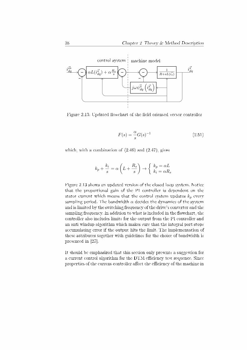
α
s= G(s)F (s) (2.50)
which means that
38 Chapter 2 Theory & Method Description
+ αL( ~isdq) + αRss + +
jω ~ψsdq
(~isdq
)1
R+sL(~is)
-
~is∗dq
-
~isdq
control system machine model
Figure 2.13: Updated owchart of the eld oriented vector controller
F (s) =α
sG(s)−1 (2.51)
which, with a combination of (2.46) and (2.47), gives
kp +kis
= α
(L+
Rss
)→kp = αLki = αRs
Figure 2.13 shows an updated version of the closed loop system. Noticethat the proportional gain of the PI controller is dependent on thestator current which means that the control system updates kp everysampling period. The bandwidth α decides the dynamics of the systemand is limited by the switching frequency of the drive's converter and thesampling frequency. In addition to what is included in the owchart, thecontroller also includes limits for the output from the PI controller andan anti windup algorithm which makes sure that the integral part stopsaccumulating error if the output hits the limit. The implementation ofthese attributes together with guidelines for the choice of bandwidth ispresented in [27].
It should be emphasized that this section only presents a suggestion fora current control algorithm for the DTM eciency test sequence. Sinceproperties of the current controller aect the eciency of the machine in
2.4 Eciency tests 39
itself, it is optimal if the test sequence uses the same current controllerwhich is used in the test objects intended application [28], [29], [30].
Final test algorithm
The subsections above give solutions for the problems that the eciencytests introduce. With the solutions in mind, the nal test sequence forthe eciency evaluation becomes
1. The maximum speed is evaluated by the preferred method (byexperimental means in this work).
2. The control system switches current control method from theDCC to FOC. The voltage drive accelerates the machine to themaximum negative speed possible with the evaluated current com-bination, but with the q current negated.
3. The control system switches sign on the q current. The drivebrakes the machine to zero speed, and accelerates it up to themaximum positive speed.
4. The drive brakes the machine to zero speed. Observe that the dcurrent (eld-weakening current) must be maintained throughoutthe braking to make sure that the induced voltage do not exceedthe DC voltage.
2.4.2 Theory of efficiency derivation
The eciency of a PMSM is dened as the the output power divided bythe input power. When the machine works as a motor, the expressionfor the eciency is
η =PmPe
(2.52)
40 Chapter 2 Theory & Method Description
where Pm is the mechanical power on the rotor shaft and Pe is theelectrical output power from the drive system. When the eciency forthe generator is calculated, Pm and Pe switches place. The electricalpower is given by (2.24), and the mechanical power is the rotor shafttorque times the mechanical frequency
Pm = Trsωm (2.53)
where the acceleration and the rotor shaft moment of inertia give theshaft torque according to (2.32). Knowing that the mechanical angularfrequency is the derivative of the rotor position divided by number ofpole pairs in the machine, (2.27), (2.53), (2.32) and (2.54) yield anexpression for the eciency
η = Jdωmdt
ωm1
uaia + ubib + ucic(2.54)
where p is the number of pole pairs in the machine.
2.4.3 Practical derivation of the efficiency from themeasurement
The eciency of a variable frequency drive machine is often presentedas a function of torque and speed. Since many dq currents achieve thesame torque and speed combination in a PMSM, the choice of torquecontrol algorithm inuences the eciency when the machine works inits application (this is especially true for salient pole PMSMs where thereluctance properties of the rotor contribute to the torque, and a isd = 0control strategy is highly inadvisable). Figure 2.14 shows the speedand torque characteristics for a typical salient pole PMSM. Numerouscurrent combinations yield the same torque and have a maximum speedwhich needs to be taken into account for. Since the dierent currentcombinations yield dierent eciencies, the rst step to derive the DTMmachine eciency characteristics is to decide which currents that shouldbe used.
2.4 Eciency tests 41
Figure 2.14: Constant torque lines and speed limit lines. Many currentcombinations yield the same torque which means that theeciency is dependent on the torque control algorithm
Figure 2.14 also shows the Max Torque Per Ampere (MTPA) trajectory,which is a well established strategy for choosing current combination.The strategy uses the minimal current which achieves the desired speedand torque [31]. The method calculates the proper dq current referencesbased on the torque equation of the PMSM, which means that themagnetic model and the resistance of the machine must be known. Inrecent schemes, online algorithms provide accurate estimation of themachine parameters for a better performing control [32], [33].
Another category of control schemes focuses on minimizing the losses.The methods use analytical expressions for the speed-dependent lossesto derive the optimal point to minimize the loss (or maximize the e-ciency) for each desired torque and speed combination [34], [35], [36].The iron losses are hard to estimate analytically due to their highlynonlinear behavior, and the accuracy of the methods can therefore bequestioned.
This work uses a method which derives the current combinations whichprovides the maximum eciency for each torque without analytical
42 Chapter 2 Theory & Method Description
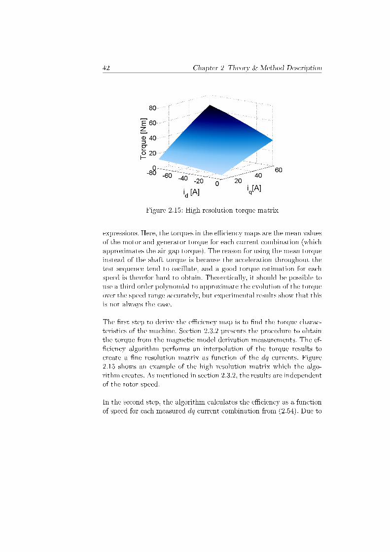
Figure 2.15: High resolution torque matrix
expressions. Here, the torques in the eciency maps are the mean valuesof the motor and generator torque for each current combination (whichapproximates the air-gap torque). The reason for using the mean torqueinstead of the shaft torque is because the acceleration throughout thetest sequence tend to oscillate, and a good torque estimation for eachspeed is therefor hard to obtain. Theoretically, it should be possible touse a third order polynomial to approximate the evolution of the torqueover the speed range accurately, but experimental results show that thisis not always the case.
The rst step to derive the eciency map is to nd the torque charac-teristics of the machine. Section 2.3.2 presents the procedure to obtainthe torque from the magnetic model derivation measurements. The ef-ciency algorithm performs an interpolation of the torque results tocreate a ne resolution matrix as function of the dq currents. Figure2.15 shows an example of the high resolution matrix which the algo-rithm creates. As mentioned in section 2.3.2, the results are independentof the rotor speed.
In the second step, the algorithm calculates the eciency as a functionof speed for each measured dq current combination from (2.54). Due to
2.4 Eciency tests 43
0 200 400 600 800 1000
0.65
0.7
0.75
0.8
0.85
0.9
0.95
speed [rpm]
Effi
cien
cy
Efficiency measurementsEfficiency fit
(a) Eciency as a function of speed forone specic current combination
(b) Maximum speeds for each currentcombination
(c) the maximum speeds at 1000 rad/s.Only the current combinationswhich have a maximum speed overthe limit may be used
(d) The torque and eciency of theavailable current combinations
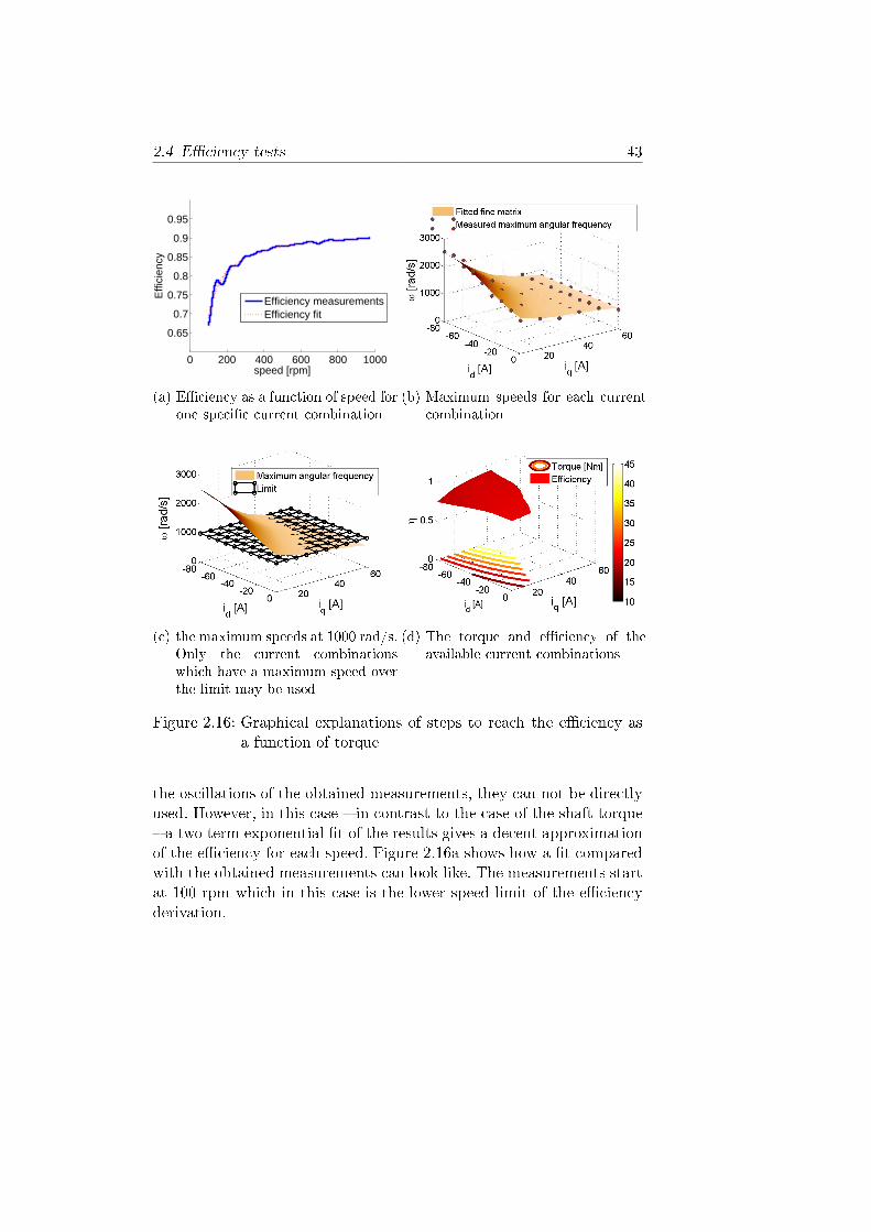
Figure 2.16: Graphical explanations of steps to reach the eciency asa function of torque
the oscillations of the obtained measurements, they can not be directlyused. However, in this case in contrast to the case of the shaft torque a two term exponential t of the results gives a decent approximationof the eciency for each speed. Figure 2.16a shows how a t comparedwith the obtained measurements can look like. The measurements startat 100 rpm which in this case is the lower speed limit of the eciencyderivation.
44 Chapter 2 Theory & Method Description
In the next step the max speed for each current combination is ttedinto a polynomial. The function gives an estimation if a current com-bination somewhere within the maximum currents can be maintainedfor a certain speed or not. Figure 2.16b shows an example of the func-tion for the measured maximum speeds and the polynomial t. Evenif the results from the pylonomial t diverges a bit from the measuredpoints, the approximation is still fairly accurate. Ideally more currentcombinations should be measured for a better result. When the maxspeed for each current combination is known, it is straight forward forthe algorithm to derive the available current combinations for the speedwhich it evaluates. Figure 2.16c shows an example of the process. Themachine only operates within the area which is above the speed limit.
With the results from Figure 2.16a and Figure 2.16c, the algorithmderives an eciency map as a function of the available mean air-gaptorque. Figure 2.16d shows the resulting eciency together with torquelines. An innite amount of current combinations create the availabletorque, but an optimization algorithm nds the current combinationswhich yield the available torques with the highest eciencies. The al-gorithm iterates through the speeds that the user desires to evaluate,and creates an eciency map as a function of torque and speed. Theeciency measurement section of chapter 4 presents a graphical repre-sentation of the end result of the procedure.
2.4.4 Power Factor
The power factor (PF) is dened as the cosinus of the angle betweenthe fundamental components of the terminal voltage and current, and isthus a measurement on how much of the apparent power from the con-verter that becomes heat and work in the machine. The most forwardway to derive the power factor is to do a Fast Fourier Transform (FFT)on each period of the measured signals and derive the phase angle inbetween them. This method can be problematic as the induced voltagecan contain a lot of harmonics especially in high eld-weakening oper-ating where the permanent magnet ux interacts with the ux createdby the d-current which leads to high frequency components in the
2.4 Eciency tests 45
voltage, and also to a certain extent in the current. This in turn makesit hard to distinguish the transition between the dierent periods in thesignals.
A way to get around this problem is to rst integrate the phase currentand voltages before deriving the angle between the fundamental com-ponents of the signals. By doing so, the high frequency components ofthe signals get attenuated, since
∫sinωt dt = − 1
ωcosωt+ C (2.55)
Figure 2.17 shows a comparison between untreated and integrated volt-age and current signals when a machine works in deep eld-weakening.The fundamental component of the voltage is barely distinguishablebefore the integration, but afterwards the fundamental is clearly dom-inating. This makes it easier for the post-processing algorithm to dis-tinguish when a new period starts as the signal does not icker aroundzero.
One aspect of this process which needs to be taken into account for is the
0 20 40 60−200
−100
0
100
200
Samples
Van [V]ia [A]
(a) Voltage and current
0 20 40 60−0.06
−0.04
−0.02
0
0.02
0.04
0.06
Samples
∫ Van dt [Vs]∫ ia dt [As]
(b) Integral of voltage and current
Figure 2.17: One fundamental period of voltage and current measure-ments in high eld weakening
46 Chapter 2 Theory & Method Description
implications of a DC oset in the measurements. An oset leads to con-tinuously growing ramps in the integrated signals. The imposed grow-ing oset makes it hard to sort out the periods for the post-processingalgorithm, and the DC component should therefor be ltered away be-fore the integration is made. Once the integrated signals without DCcomponents is derived (Figure 2.17b), the number of samples betweenthe peaks of the fundamental frequencies of the signals gives the phaseshift ( supposing the number of samples for the whole period equals 360degrees). The fundamental frequency can for example be obtained bya FFT; this work's post-processing algorithm derives the fundamentalwith the matlab "sum of sines" function which is closely related to thediscrete Fourier transform.
An alternative method derives the PF from the transformed dq volt-age and current. The dq transformation yields the same angle between~udq and ~idq as between the terminal voltages and currents. Therefore,cosinus of the absolute value of a subtraction between the voltage andcurrent angle in regard to the d axis in the dq frame gives the powerfactor
cos(φ) = cos(θudq − θidq
)(2.56)
Since the current and voltage always exist in the second or third quad-rant in the dq frame (the current is always in the third, but the voltagecan exist in the forth if the negative d current gives rise to a ux whichis greater then the permanent magnet ux), the current and voltageangle in respect to the d axis are given by
θudq = tan−1(uqud
)+ π
θidq = tan−1(iqid
)+ π
2.4 Eciency tests 47
The benet of this method compared to the procedure which derivesthe PF directly from the phase voltages and currents is that ~idq staysconstant throughout the tests. Furthermore, the voltage changes fairlylinearly with speed. This makes it easier to lter the signals, and thepost-processing algorithm becomes less complicated.
2.4.5 Loss separation
The losses in a PMSM can be divided up in three main parts
1. Resistive stator winding losses. These losses are practicallyassumed to be independent of frequency, even though this is nottrue since the proximity and the skin eect aect the resistance.The resistivity of the conductor is also highly temperature de-pendent, which leads to a change in the losses when the windingsheat up.
2. Losses in the core. The core losses are often divided up in threecategories: hysteresis, eddy current and excess losses [37]. Hystere-sis losses occur because of the non-linearity between the currentin the winding and the ux density in the core; the magnetiza-tion and demagnetization of the core yield dierent relationshipsbetween the magnetic eld strength (proportional to the current)and the magnetic ux density. This creates energy demandinghysteresis loops which manifest as losses in the machine. The hys-teresis losses are assumed to be proportional to the frequency ofthe ux density.
The eddy current losses are due to induction in the core alloywhich the time varying magnetic ux density gives rise to. Thecore is usually laminated to limit this phenomenon, but when thefrequency is high the eddy currents still cause considerable lossesin the machine. These losses are proportional to the square of thefrequency.
The excess losses occur when the ux density which the stator
48 Chapter 2 Theory & Method Description
current and permanent magnets give rise to interacts with thehighly inhomogeneous ux created from the induced eddy currents[37]. The losses are approximately proportional to the frequencypowered by one point ve in most core materials.
3. Mechanical and windage losses. The mechanical and windagelosses consists of bearing and air friction and depend on the prop-erties of the bearings, the shape of the rotor and the air-gaplength. Approximately, the bearing friction losses depends linearlyon the frequency while the windage losses have a cubic relation-ship to it.
A rst step in the loss separation process is to divide the losses whichbrakes the rotor of the machine with the losses that are due to thestator current. The losses which brake the machine give rise to a losstorque, which may be derived by subtracting the mean air-gap torque(Tmag) from the rotor shaft torque (if ux leakage is neglected). This losstorque includes all speed dependent losses in the machine. Since the ux,currents, acceleration and moment of inertia of the rotor axis are known,the loss torque can be derived directly from the DTM measurements
Tloss =(isqψ
(isd,isq)
d − isdψ(isd,i
sq)
q
)− J dω
dt(2.57)
Supposing that the windage losses are negligible, the power losses whichbrake the machine can be approximated by
PTloss = Kfωm +Khpωm +Kexcpω1.5m +Kepω
2m = Tlossωm (2.58)
where p is the number of pole pairs, Kf is the friction loss coecientand Kh, Kexc and Ke are iron loss coecients. Since the power is thetorque times the speed, the expression for the loss torque becomes
Tloss = Kf +Khp+Kexcp√ωm +Kepωm (2.59)
2.4 Eciency tests 49
The equation above shows that the friction and the hysteresis lossesintroduce a constant braking force on the rotor axis, while the excessand eddy current forces increase with speed. The expression does notallow for a separation between the friction and the hysteresis losses.Even so, it is possible to nd the eddy current and excess loss coecientsif the evolution of the loss torque is examined.
Ideally, the loss torque includes all losses except for the losses in thecopper. This is not entirely true since the resistance in the stator wind-ings is frequency dependent. With that being said, if the coils are madeup of litz wire, the skin and proximity eects are attenuated to thepoint where the frequency dependence can be neglected. In that case,the resistance introduces a constant loss which easily can be separatedfrom the speed-dependent losses.
The retardation method
A complementing measurement procedure which can be combined fairlyeasily with the DTM without the need to introduce more equipment,is the retardation method. The IEEE standard for testing synchronousmachines suggests this method to nd the rotor iron and friction losses.This is the measurement procedure: The machine is accelerated up tobase speed whereupon the phases are disconnected from the converter.After the disconnection, the machine decelerates due to losses. If therotor position is measured during the procedure and the moment ofinertia of the rotor shaft is known, the losses can be derived from theequation of the rotor shaft torque. Since the electromagnetic torque andthe load torque are zero, the change of speed and the moment of inertiagive the loss torque directly.
Since the magnetization cannot be turned of in a PMSM, it is not easyto separate the iron losses that are induced by the permanent magnetux from the friction losses. The only way to get around this problemis to rst test the machine with a rotor without permanent magnets,and then exchange it for the PM rotor. Even so, the retardation teststill gives valuable information of the open circuit characteristics of the
50 Chapter 2 Theory & Method Description
machine. It can be specially interesting to compare the open-circuit losstorque with the loss torque that occur during loading. This can give aclue on how the stator current ux interacts with the ux from thepermanent magnets.
Conclusions
The loss separation procedure of the DTM is still under development,and the ideas which this section presents have not yet been evaluated.Even so, The DTM has potential to be useful for these kind of purposes,in addition to providing ux and torque characteristics of a machine.
2.5 Measurement considerations
This section discusses dierent measurement considerations from themagnetic model derivation point of view. Even so, much of the infor-mation is also valid for the eciency measurements and loss separation.A more elaborate discussion regarding the data acquisition and treat-ment for the eciency measurements is a topic for future research.
2.5.1 data acquisition
Rotor position
A high precision rotor angular position measurement is important foraccurate DTM results. Hypothetically, the position is not needed forthe derivation of the ux if the angular speed of the rotor and thevoltages in the dq frame are available. However, the dq transformationsin the control system still need accurate rotor position measurements toprovide reliable variables. As it is easier to process data o-line, boththe frequency which is the derivative of the position and the dq
2.5 Measurement considerations 51
currents and voltages are derived from the measured position in thescheme which this thesis presents.
Most high accuracy and cost eective angular position sensors give twosinus waves in quadrature relationship to provide information about therotor position [38]. The position sensor of the test machine which chap-ter 3 presents is a resolver, which, given an excitation signal, providesthe sine waves with information about the position. In addition to therotor position information, the signals from the sensor also carry har-monics with the same frequency as the excitation. The resolver signalsmust therefor be demodulated to obtain the rotor position. Throughoutthe experiments in this work, the demodulation process underwent withthe assumption that the high frequency components of the resolver sig-nals and the excitation signal were in phase. Under such circumstance,the excitation signal can be used directly in the demodulating process[39], [40]. In the procedure that was used during this work, the demod-ulation algorithm nds the peaks of the resolver signal high frequencycomponent; mr Yury Loayza designed and implemented the code forthe demodulation.
The process of deriving the position after the demodulation is straightforward. Supposing ideal steady-state resolver signals, they can be ex-pressed mathematically as
uresd = |u| cos θ sinωext (2.60)
uresq = |u| sin θ sinωext (2.61)
where θ is the rotor position and sinωext is the high frequency excita-tion component. The demodulation process removes the high frequencycomponent, and the expressions for the demodulated resolver signalsbecome
uresd = |u| cos θ (2.62)
uresq = |u| sin θ (2.63)
The rotor position can now be directly obtained with the arcus tangens
52 Chapter 2 Theory & Method Description
function
θ = arctanuresquresd
(2.64)
To avoid zero division problems with the expression above, theta maybe derived with the coordinate rotational digital computer (CORDIC)algorithm [41]. The CORDIC algorithm iterates through dierent anglesby rotating the measured vector (cos θ + j sin θ) back and forth untilthe argument is approximately zero (the accuracy of the procedure isrelated to the number of iterations the algorithm performs). The actualposition can be derived since the algorithm knows how many degreesthe measured vector rotates throughout the procedure. The algorithmis suitable to implement on eld programmable gate arrays (FPGAs)and derived the rotor position during the experiments.
A control loop which suppresses the error of the angle gives an alterna-tive way to obtain the rotor position. The algorithm derives the cosinusand sinus of the estimated angle, whereupon (2.62) is multiplied by theestimated sinus, and (2.63) is multiplied with the estimated cosinus. Asubtraction of the two multiplications together with trigonometric op-erations yield an estimation of the error. The error is then suppressedby a loop similar to a phase locked loop. This procedure was not usedfor the experiments presented in chapter 4, but many papers recom-mend it for a more reliable and stable angle derivation [39], [40], [42],[43], [44].
Voltage
The converter phase voltage is maybe the most challenging DTM vari-able to obtain. The literature presents a couple of solutions: Analog inte-grator circuit methods integrate one switching period and thus providethe quasi-instantaneous mean value of the voltage [45], [46], [47]. Theprocedures give accurate results, but the circuits need time-consumingmanual tuning, and the value of the passive components tend to drift
2.5 Measurement considerations 53
UaN
+
-
UDC
+
-
(a) Voltage measurement clari-cation
UaN
UbN UcN
Uan
Ubn Ucn
+
-
-
+
-
+
(b) Simple equivalent model
Figure 2.18: Converter and machine voltages dened
with temperature. Digital integration also provides high accuracy mea-surements: High speed high accuracy analog to digital (A/D) convertersobtain the instantaneous voltages and a digital circuit, typically a eldprogrammable gate array, performs the integration [48]. The procedureavoids the manual tuning and temperature dependence of the analogcircuits, but the high speed, high precision A/D converters are costly. Athird phase voltage estimation strategy is to use the current controllerreference value as DTM data. The switching dead-time, the rise an falltime, and the voltage drop over the semi-conductors in the convertermust be taken into account for accurate estimations [49],[50],[51]. Thestrategies are designed for a constant switching frequency, and they donot work with the current control strategy of the DTM magnetic modelderivation.
The strategy which was used during the measurements in this projectobtains the voltages by controlling the voltage level in between theconverter leg's transistors while at the same time keeping track of theDC link voltage. The method has been evaluated before, but withouttaking voltage drops over the converter semiconductors into account[52]. Figure 2.18a helps to describe the strategy: Dierential probesmeasure VaN , VbN and VcN , which are the phase to DC link neutralvoltages. Since high speed and high accuracy analog to digital convertersare costly, the three probes are connected to a very high speed digitalinputs; the measurements provide information regarding the state of
54 Chapter 2 Theory & Method Description
each phase leg.
While the DAQ system obtains information regarding the phase legstates, a sensor together with an high accuracy but low speed analogto digital (A/D) converter collects DC link voltage measurements. Thesampling speed of the A/D converter can be slow as the change ofthe dc-link voltage is limited by the DC link capacitor. Since VN isapproximately VDC when the upper transistor conducts, and zero ifnot, a multiplication between the state of a phase leg and Vdc givesan approximation of VN . The dierential probes measure the actualswitching of the transistors and the necessary switching dead-times,when both transistors in one leg are turned of, are therefore taken intoaccount. On the other hand, the voltage drop over the transistors andfree-wheeling diodes still introduce errors in the measurements. Theexpressions for the converter leg voltage over one period without takingthe semiconductor voltage drops into account become
UN =1
N
N∑k=1
δ(k) · Udc(k) (2.65)
where δ is the state of the converter legs. To reduce the transistor anddiode voltage drop errors, they are added or subtracted from UN : If theupper transistor conducts and the phase current is positive, the voltagedrop over the transistor is subtracted from UN . If, on the other hand, thecurrent is negative, the voltage drop over diode is added to UN . Whenthe lower transistor conducts, the voltage drop of the diode is added ifthe current is positive, and the transistor voltage drop is subtracted ifthe current is negative. This error reduction demands that the on statevoltage drop over the semi-conductors are known. As the voltage dropsare functions of the current, this compensation procedure is not trivialto perform. The voltage drops can be expressed mathematically as
2.5 Measurement considerations 55
Udrop(x) =
+Utrans, i < 0, δ = 1+Udiode, i > 0, δ = 1−Utrans, i < 0, δ = 0−Udiode, i > 0, δ = 0
and (2.5.1) together with (2.65) yield a rened expression for the con-verter leg voltage
UN =1
N
N∑k=1
δ(k) · Udc(k)− Udrop(k) (2.66)
Figure 2.18b shows a simplied equivalent circuit of the machine. OnceUaN , UbN and UcN are obtained, Kirchos voltage law (KVL) yield thephase voltages in regard to the Y connected machine neutral
Uan =2
3
(UaN −
UbN2− UcN
2
)(2.67)
Ubn =2
3
(UbN −
UcN2− UaN
2
)(2.68)
Ucn =2
3
(UcN −
UaN2− UbN
2
)(2.69)
These are the voltages that are used to derive the linked magnetic uxin the magnetic model derivation.
Current
The DTM demands high precision instantaneous current measurementto give good results. The IEEE standard for measurements in power cir-cuits describes some approaches to obtain the current [53]. One of these
56 Chapter 2 Theory & Method Description
procedures uses Hall sensors, which measured the current throughoutthis work's experiments. The Hall sensor does not intervene directlywith the current path. Instead, it is placed around the conductor, andthe magnetic eld which the current gives rise to induces a voltage inthe sensor.
After the voltage is induced, an op-circuit amplies the signal to suitthe level of the analog to digital converters of the control system. Theamplier circuit is prone to introduce some level of oset, and a per-fectly symmetric amplication of the three phases can not be taken forgranted. The control system needs to compensate for these imperfec-tions for good results; section 2.5.3 discusses this further.
2.5.2 Post-processing
The post-processing procedure after the measurement data is acquiredis not part of the conceptual idea of the dynamic test method. Withthat being said, it may be interesting for the reader to get an idea ofhow the data can be processed to reach a satisfying result. This sectionshows an example of how measurement data can be processed, and alsohow the results presented in chapter 4 were derived.
Rotor position and electrical frequency
Figure 2.19a shows an example of measured rotor positions throughouta test cycle. The measurements span between minus pi and pi, where oneperiod is two pi. To make it easier to process the data, the samples arestacked on top of each other (Figure 2.19c). This leads to a smooth curvewhich can be low-pass ltered to reduce noise of the obtained position.Figure 2.19d shows a zoomed in example where the measurements (theblue dots) are ltered (the red line).
The choice of low-pass lter algorithm for the position has a big in-uence of the outcome of the ux derivation: If the lter is to fast,
2.5 Measurement considerations 57
0 5 10x 10
4
−4
−2
0
2
4
Samples
θ [r
ad]
(a) Measured angle
4 4.02 4.04 4.06 4.08x 10
4
−4
−2
0
2
4
Samples
θ [r
ad]
(b) Measured angle zoom in
0 5 10x 10
4
−800
−600
−400
−200
0
Samples
θ [r
ad]
(c) Stacked angle
4.404 4.4045 4.405 4.4055x 10
4
−258.4
−258.2
−258
−257.8
−257.6
Samples
θ [r
ad]
(d) Spline t angle
Figure 2.19: Measured rotor position
the ickering in the position measurements leads to a big ripple in thefrequency estimation. If, on the other hand, the lter is to slow, thelow-pass ltered position will not follow the actual position when therotational direction changes (this is where the position change the most,which also is the minimum point in Figure 2.19c). In the results whichchapter 4 presents, a spline interpolation lters the signal.
The spline interpolation works well as it follows the measured positionwith a low degree polynomial which is robust against high frequencynoise in the signal. The spline is divided up in several segments, andan interpolation is done within each. For the results that chapter 4,the matlab function splinet by mr. Jonas Lundgren interpolated themeasured rotor position data.
58 Chapter 2 Theory & Method Description
0 5 10x 10
4
−2000
−1000
0
1000
2000
Samples
ω [r
ad/s
]
(a) Angular frequency from raw angle
0 5 10x 10
4
−1000
−500
0
500
1000
(b) Angular frequency from spline t-ted angle
0 5000 10000 15000
−500
0
500
Samples
ω [r
ad/s
]
(c) Measurements used for the magnetic model derivation
Figure 2.20: Speed derivation
To show how important it is to low-pass lter the position, Figure 2.20apresents the angular frequency derived from the non-ltered position,while Figure 2.20b presents the frequency estimated from the lteredsignal. The derivative of the raw position estimation has a very bigripple due to the noise of the raw measurements while 2.20b shows asmooth curve. Figure 2.20c displays the cropped speed range, which isthe data the magnetic model derivation algorithm uses.
Voltage
Figure 2.21a shows measurements of UaN (see Figure 2.18) through-out a test sequence. The harmonic content of the voltage is very high.
2.5 Measurement considerations 59
Furthermore, the amplitude varies throughout the test sequence. Theharmonics are apart from a non-sinusoidal induced voltage due tothe variable frequency of the current controller. The variations of theamplitude are due to the rotating converter that supplies the test rigwith the DC-link voltage. This is an unwanted phenomenon, but itis specic for the setup that was used throughout these tests, and istherefore not an intrinsic behavior of the method itself. The raw mea-surements UaN , UbN and UcN , together with (2.67), (2.68) and (2.69),yield Uan, Ubn and Ucn. Figure 2.21b shows that high harmonic contentremains after the derivation.
Uan, Ubn and Ucn remain unltered when they, together with (2.1),(2.2) and the raw measurements of the rotor angle, give the dq voltages.Figure 2.22a shows that the harmonic content of the resulting d voltageis, as expected, very high; the same is true for the q voltage. Figure2.22a also displays another interesting phenomenon: The change overtime, if the harmonics are disregarded, is much slower compared to theUN and Un voltages. Because of this, a low-pass lter works better onthe dq voltages than the phase voltages, as the time constant can belower without aecting the fundamental component of the signals.
Figure 2.22b shows the d voltage after it is low-pass ltered with samespline algorithm that lters the rotor position measurements. The volt-age changes nearly linearly with time, which is expected as the inducedvoltage is linearly dependent on the electrical frequency.
Current
The post-processing of the current is straight forward. The obtainedrotor position together with the dq transformations yield the currentin rotor coordinates. Since the currents play no explicit role in the uxderivation, their function is to show that the measurements are correct.If the currents are noisy, they may be ltered to control that the quasi-instantaneous values are correct.
60 Chapter 2 Theory & Method Description
0 5 10x 10
4
0
100
200
300
Samples
VaN
[V]
(a) Measured UaN
0 5 10x 10
4
−200
−100
0
100
200
Samples
Va [V
]
(b) Derived Uan
Figure 2.21: Raw converter voltage and machine phase voltage mea-surements
0 1 2x 10
4
−200
−100
0
100
200
Samples
Vd [V
]
(a) Raw d voltage
0 0.5 1 1.5 2x 10
4
−40
−20
0
20
40
Samples
Vd [V
]
(b) ltered d voltage
Figure 2.22: d voltage
2.5.3 Measurement errors
Position measurements
Errors in the rotor position estimation when performing dynamic testscan have great inuence on the end results. The errors can manifestas a ripple and/or an oset. Oset errors are the most severe as theyintroduce a shift in the dq reference frame. Figure 2.23 shows a possiblescenario when an oset error is present. The shift in angle makes thetransformed dq currents dier from the reference currents, and the ux
2.5 Measurement considerations 61
d
q
θ θ∗
Figure 2.23: Shift in the dq coordinates due to oset in the resolvermeasurements. θ∗ is the reference angle and θ is the error
maps are thus shifted. The oscillating errors may inict torque ripple,but since many measurements are obtained and averaged over a DTMtest sequence, they do not aect the results in a signicant way. Themeasurement procedure can be divided up in three stages which canintroduce errors:
1. There exist disturbances in the signals generated by the resolver.The resolver signals always contain noise and asymmetry to a cer-tain extent. This may have a non-negligible eect on the demodu-lation process and position measurement if the imperfections aretoo prominent. The most common resolver signal errors can bedivided up into six categories, where two are of great signicanceto the DTM [42]:
a) The two resolver signals are not in a perfect quadrature. Thisimposes both an oscillating error and an oset error in theposition according to ε = −β
2 (1 − cos 2θ), where β is thephase shift which makes the signals deviate from a quadra-ture relationship, and θ is the rotor position. A correctionprocess of this type of errors is described in [43].
b) The excitation signal and the high frequency component of
62 Chapter 2 Theory & Method Description
the returning resolver signals are not in perfect synchroniza-tion. This error is unavoidable due to the resistance of theresolver windings. The phase shift introduces an error whichis dependent on the change of the resolver angle according
to ε = θω δ, where ω is the electrical radial frequency and δ is
the excitation signal phase shift. A demodulating procedurethat cancels this error is presented in [44].
2. The demodulation process together with the angle derivation fromthe demodulated signals introduce errors due to noise sensitivity.These errors introduce ripple in the position estimation, but doesnot inict a permanent oset, and they do not create to muchcomplications for the DTM.
3. The resolver can be poorly calibrated, which means that the d-axis is not perfectly aligned with the permanent magnet ux.This introduces a constant oset in the angle which, as mentionedbefore, aects the results of the DTM.
Since an error in the angle imposes a rotation of the reference frame,the impact of it depends on the characteristics of the machine, and aquantitative estimation of how much a specic error aects the testresults is therefore impossible to make.
Voltage
The voltage is the only DTM variable which does not take an active partin the control system. The testing performance is therefor unaected byan error in the voltage. With that being said, errors in the measurementsstill have an impact on the magnetic model and eciency derivation.The possible reasons for measurement errors neglecting sources such asrise/fall time of the semi-conductor devices and voltage ickering/overshoots, which are impossible to detect with the used method may bedivided up in three categories:
2.5 Measurement considerations 63
1. The dierential probes or the digital sensors fail. When this hap-pens, the converter leg measurements are lost and the tests mustbe remade.
2. The DC voltage measurements are badly tuned. Since the DTMdoes not aect the test procedure, an estimation of the eect ofan error in the DC voltage measurement can be reached in thepost-processing. Supposing an error factor αe, and neglecting thevoltage drop over the converter components, the converter legphase voltages become
UN = αeUdcδN = αUN (2.70)
UN together with (2.67)-(2.69) yield
Un = αeUn (2.71)
The dq transformations are linearly dependent on the amplitudeof the variables that are being transformed if they are symmetric.The expression for the dq voltages thus becomes
udq = αeudq (2.72)
Finally, the derived voltages together with (2.22) and (2.23) showthat
ψdq = αeψdq (2.73)
This expression holds for both a gain and a oset error since theDC- link value is considered constant. If the DC-link voltage dropsthroughout the sequence, a gain error changes while an oset errorremains the same. As long as the voltage drop is not severe, the
64 Chapter 2 Theory & Method Description
change of the gain error is very small and can be neglected, and(2.73) therefor holds.
3. The estimations of the voltage drops over the components in theconverter are wrong. The errors are functions of both the state ofthe of the voltage legs and the sign of the currents. If the factorof the error is denoted βe, the new expression for the converterleg voltage is expressed as
UN =1
N
N∑k=1
αe · δ(k) · Udc(k)− βe(k) · Vdrop(k) (2.74)
Note that αe is independent of the position sample of the inte-gration while βe as can be seen in (2.5.1) is. This makes itimpossible to estimate the inuence of βe in the post processing.With that being said, the inuence of β is much less than αe, andhas very little inuence on the end result of the measurements.
Current
In contrast to the voltages, errors in the current measurements aectthe on-line performance of the DTM testing process directly. There aretwo common errors which can occur during the measurement procedure[54]:
1. One or many of the sensors, measurement circuits and/or A/Dconverters imposes an oset on the provided signals.
2. The gains of one or more of the signals are wrong.
Figure 2.24 shows what happens when the dierent errors are imposedon one phase of a perfectly symmetric three phase system. An oseterror adds an oscillating component to the dq currents. As the controllertries to keep the d and q current constant, it makes the amplitude of
2.5 Measurement considerations 65
one of the phase currents oscillate. This imposes a torque ripple on themachine.
An asymmetric gain error both imposes an oscillating signal, and givesrise to an oset in the currents in the rotor reference frame. Since thecontroller tries to keep the measured current at the reference value, theactual tested combination varies with time. Even more importantly, itoscillates around a rotor reference current which deviates from the onethe control system aims to evaluate. This means that the ux maps thatthe algorithm derives apply to unknown current combinations whichdeviate from the intended. Caution should therefor be taken to adjustthe gains of the currents in the control system to accurate values.
0 5 10−10
−5
0
5
10
θ rad/s
i dq [A
]
id
iq
id offset
iq offset
id gain
iq gain
Figure 2.24: Inuence of errors in the current measurements
Chapter 3
Experimental Setup
Figure 3.1 shows how the equipment was set up for the experimentaltests. A central control and DAQ system controls the converter whichdrives the test machine. A resolver sensor provides the necessary infor-mation about the rotor's position. Hall sensors measure the currents,and voltage probes give the duty cycle of the phase voltages as describedin chapter 2.
A DC machine driven mechanically by an asynchronous machine pro-vides the voltage on the DC side of the converter. As the DC machineworks both as a motor and as a generator, the DC link is able to ab-sorb as well as provide electrical energy. This feature is, as mentioned inchapter 2, essential for the dynamic test method to work; an ordinaryDC rectier can therefor not be used for this method.
3.1 Control and DAQ unit
National instruments compact rio system (cRIO) was used to controlthe converter voltage and to gather data throughout the testing. Thesystem includes a real-time system and a eld programmable gate array(FPGA) together with an interface to a personal computer. In addition,integrated slots for in and out modules make it easy obtain data andto communicate with the outside world.
68 Chapter 3 Experimental Setup
=≈
vNabc
iabc
Control
&DAQ
δ∗vabc
= Dierential probe
= Machine
=≈ = Converter
Figure 3.1: Experimental test setup
The FPGA part of the cRIO is a desirable platform for control and datacollection due to its precise timing and true parallelism, but space andmemory restriction limits the amount of code that can be executed onit. Functions which are in need of timing and speed performance, suchas current control, were therefor implemented on the FPGA, while thecontrol of the entire test sequence which is less time critical wasimplemented on the real-time part of the system. A rst in rst out(FIFO) communication sent the measurement data from the FPGA tothe PC where it was stored for data post-processing.
3.2 Setup for constant speed tests
To compare the results form the dynamic test measurements with re-sults from a more established test procedure, a setup was created forconstant speed tests. Figure 3.2 shows the design of the setup. Com-
3.3 Test object 69
δ1,2∗vabc
Udc+
−=≈
=≈
vNabc
i1abc i2abcControl
&DAQ
Figure 3.2: Experimental test setup for constant speed tests
pared to the dynamic test setup (Figure 3.1), an additional machine isintroduced and connected mechanically to the test object. The machineworks as a generator if the test object is tested as a motor, and as amotor if the test object is evaluated as a generator. A second convertercontrols the new machine.
Because of the new machine, the speed of the test object can be heldconstant independently of the torque it produces (supposing that thenew machine is strong enough). In this works setup, the additionalmachine was very similar to the test object, which made it possible toperform the tests over a wide speed and torque range. Figure 3.3 showshow the test object and the second machine was assembled. There wasalso a torque sensor mounted in between the machines, but it was notused for the tests presented in this work.
3.3 Test object
Figure 3.4 shows the design of the test object. The machine is an eightpole permanent magnet machine with integrated magnets designed byDr. Fransisco J. Márquez-Fernández for an electrical rear wheel driveunit. Due to the integrated magnets, the saliency of the machine (the
70 Chapter 3 Experimental Setup
Figure 3.3: Setup for constant speed tests
dierence of inductance in d and q) is relatively high. The machineis designed for 20 kW continuous power with an overload capability ofthree times, and a maximum speed of 15000 rpm with a eld weakeningratio of 1:5. More information regarding the design of the machine canbe found in [55].
The machine features various integrated pt100 temperarure sensorsmounted in dierent locations. The sensors give information about thewinding, iron, and to a certain extent permanent magnet temperature.This information is valuable since material characteristics such as theresistivity of the copper and magneto-motive force of the permanentmagnets change when losses heats up the machine. In this work, onlythe winding temperature sensor, denoted with blue circles in gure 3.4,was used; in a more excessive study it would be interesting to monitorthe permanent magnet temperature also (this was not performed dueto lack of time). A thorough investigation of the temperature propertiesof the machine is found in [56].
3.4 Equipment for rotor moment of inertiaderivation
To be able to nd the rotor moment of inertia three ywheels withdierent moment of inertia was custom made for the test object. Inaddition, a triliar pendulum was created to measure the moment of
3.4 Equipment for rotor moment of inertia derivation 71
Figure 3.4: Placement of pt100 sensors. Taken from [56], with permis-sion
inertia of the ywheels. The equipment that was used to derive therotor moment of inertia is seen in gure 2.10 in chapter 2.
Chapter 4
Experimental Results
This chapter presents results from experimental tests performed withthe dynamic test method. Since many experiments have been performedthroughout the project, the current range of the results vary. Generally,the sections show the material in the same way that it is presented inpublications, and a lot of the results in this chapter can therefore alsobe found elsewhere. The purpose of this chapter is rst and foremost tostring together the dierent parts and give a coherent overview of theresults.
4.1 Magnetic Model identification
4.1.1 The magnetic model
Figure 4.1 shows the resulting ux maps from the DTM tests. Thelinked magnetic d ux (Figure 4.1a) is about 0.125 Weber without eldweakening current. A negative d current gives rise to a ux which op-poses the one from the permanent magnets, and the resulting d uxlinkage therefor decreases. When the negative d current is big enough,it cancels out the ux from the permanent magnets entirely, whichmeans that ψd is zero, and torque is only generated due to the mag-netic asymmetry of the rotor (reluctance torque).
74 Chapter 4 Experimental Results
−100−50
0 050
1000
0.05
0.1
0.15
iq [A]i
d [A]
ψd [W
b]
0.04
0.08
0.12
(a) d ux
−100−50
0 050 100
0
0.1
0.2
iq [A]i
d [A]
ψq [W
b]
0.1
0.15
0.2
(b) q ux
Figure 4.1: Linked ux as functions of the d and the q currents
The estimated q ux (gure 4.3b) is, in contrast to the d ux in regardto the d current, highly nonlinear in regard to the q current. This isdue saturation in the iron core. The nonlinear behavior makes it un-tting to express the relationship between the current and the ux asan inductance (as a matter of fact, this phenomenon is the reason whythe magnetic model in this work is presented as ux maps and not asinductance maps).
4.1.2 Comparison with results from FEMM simulations
Figure 4.2 shows comparisons between results from a 2D FEM simula-tions on the machine and the results from the DTM. The q ux resultst well (Figure 4.2b), while the DTM derives lower values than the sim-ulation for the d ux (Figure 4.2a). The reason for the discrepancy inthe d ux is not obvious, but possible reasons are a too low reluctancein the d axis magnetic circuit in the FEMM model, that the magneto-motive force in the permanent magnets are modeled to high or thatthe simulations does not take the end-turn inductance of the machineinto account. A more elaborate discussion regarding this phenomenonis found in [57].
The simulation model of the test object was already nished by Dr.
4.1 Magnetic Model identication 75
(a) d ux (b) q ux
Figure 4.2: Comparison between the magnetic ux linkage model de-rived by the dynamic test method (blue surface) and fromFEMM simulations (yellow surface)
Francisco J. Marquez-Fernández before DTM experiments were con-ducted. All post-processing of the simulation results from the FEMMsimulations was made in matlab; the post processing code was writtenas a joined eort of the IEA section in Lunds University. The authorhas not taken part of the writing of the code, but the code and modelwas used in consent with the creators. A detailed presentation and ex-planation of the simulations is found in [55].
4.1.3 Comparison with results from a constant speedmethod
In addition to the DTM tests, the test object was also evaluated withan established constant speed method (CSM) for comparison purposes.The test procedure of the CSM goes as follows: The speed of the testobject is held constant by an additional brake machine while the de-sired current combination is applied. Many periods of the voltage andposition are measured for each dq current combination, and the result-ing voltages in dq are calculated from the measurements o-line. Thederived voltages are very noisy due to harmonics in the induced voltagewhich the ux from the permanent magnets and the applied currentsgive rise to, and the results must be averaged over time for an accurate
76 Chapter 4 Experimental Results
−100−50
0 050
100
0
0.05
0.1
0.15
iq [A]i
d [A]
ψd [W
b]
DTMCSM
(a) d ux (b) q ux
Figure 4.3: Comparison between estimated ux from the constant speedmethod and the dynamic test method
ux estimation.
The theory of the CSM is based on the ux equations of the PMSM.Since the setup measures the voltages and currents, the only unknownvariable in the equations is the stator resistance. This resistance is nottrivial to estimate as it changes with temperature. In this case, it ismeasured with a high resolution multimeter at many temperatures.Since the winding temperature is monitored continuously throughoutthe tests, the change of resistance can be taken into account in the datapost-processing procedure.
Result comparisons
Figure 4.3 shows the magnetic ux linkage when the CSM derives theresults compared with the DTM results. The results t quite good, butthe d ux diverges with a big q current and vice versa. The dierencein the results can be explained by the change in ux linkage when themachine works in motor operation compared with generator operation(the dierence occurs due to core losses, as explained in chapter 2).Since the results from the CSM is derived when the machine works asa motor, while the DTM results are obtained from measurements when
4.1 Magnetic Model identication 77
−100−50
0 050
100
0
0.05
0.1
0.15
iq [A]i
d [A]
ψd [W
b]
CSM
DTM
(a) d ux
−100−50
0 050
1000
0.1
0.2
iq [A]i
d [A]
ψq [W
b]
CSM
DTM
(b) q ux
Figure 4.4: Comparison between estimated ux from the constant speedmethod and the dynamic test method using measurementsonly from the motor part of the sequence
the machine works both as a generator and motor, a small dierence isexpected.
To make a fairer comparison, new maps are obtained from the DTMusing only measurements from when the machine works in motor oper-ation (when the machine accelerates). A rewrite of the PMSM voltageequations ((2.16) and (2.17)) yields the linked ux from the measure-ments. Figure 4.4 shows a comparison of the new DTM ux maps to-gether with the results from the CSM. The results ts almost perfectly;there still exists a small oset in the q ux when the q current is small,but as gure 4.4b shows, it is marginal.
It should be mentioned that the results point towards an unrealisticallybig dierence in the ux linkage when the machine works in motoroperation compared with generator operation. Chapter 5 discusses thisphenomenon further.
78 Chapter 4 Experimental Results
Temperature comparison
Figure 4.5 shows d ux linkage results from the DTM and CSM mea-surements at two dierent stator winding temperatures. The same sta-tor winding resistance value is used for both temperatures. The resultsfrom the dynamic measurements (gure 4.5a) shows an almost con-stant oset between the ux lines when the winding temperature dieraround 35 degrees Celsius the warmer machine links slightly less uxthan the cooler. With higher q currents than around 70 Amperes, theux lines start to diverge. A possible reason for the constant oset iswarmer magnets which leads to less ux density. The reason for thediversion at higher q currents is unknown. Looking at the results fromthe CSM, the ux lines from the two temperatures are tilted slightlydierent (gure 4.5b). This is explained by (2.16): A too low resistancevalue leads to an overestimation of the ux. The phenomenon is espe-cially apparent for big q currents, where the results make you believethat a hotter machine links more ux than a cooler.
Figure 4.6 shows estimations of the q ux. The results from the DTM areapproximately the same independently of winding temperature (gure4.6a). This is true except for when the q current is very high, where just as with the d ux (gure 4.5a) the hot machine links slightly lessux than the cold. The CSM results (Figure 4.6b) diverge when the dcurrent is high. This is due to the resistive voltage drop in (2.17), which,when a too small value is used, leads to a too high ux estimation.
4.1.4 Winding temperature development
If the DTM results should be independent resistive voltage drop, thewinding resistance, and hence also the winding temperature, cannotchange much during one test cycle. Figure 4.7 shows the change in theresistance in a resistance thermometer (PT100) which is mounted on aphase winding. The current combination isd = −100A and isq = 10A ischosen for the test as it gives the least torque for the most current; thisis the worse case scenario in terms of heating of the windings during
4.1 Magnetic Model identication 79
−100 −50 0
20
40
60
80
100
i q [A]
id [A]
ψd [Wb]
0.02
0.04
0.06
0.08
0.1
0.12T=45−50oC
T=80−85oC
(a) Dynamic test method results
−100 −50 0
20
40
60
80
100
id [A]
i q [A]
ψd [Wb]
0.02
0.04
0.06
0.08
0.1
0.12T=80−85oC
T=45−50oC
(b) Constant speed method results
Figure 4.5: d Flux estimation from the dynamic method and the con-stant speed method at two dierent temperatures. The sta-tor resistance value is assumed to be constant
−100 −50 0
20
40
60
80
100
ψq [Wb]
id [A]
i q [A]
0.1
0.15
0.2T=80−85oC
T=45−50oC
(a) Dynamic test method results
−100 −50 0
20
40
60
80
100
ψq [Wb]
id [A]
i q [A]
0.1
0.15
0.2T=45−50oC
T=80−85oC
(b) Constant speed method results
Figure 4.6: q Flux estimation from the dynamic method and the con-stant speed method at two dierent temperatures. The sta-tor resistance value is assumed to be constant
one test cycle. The temperature change in the PT100 is approximately0.15 Ω, which translates into 0.4oC. The change is negligible and theassumption that the winding resistance remains constant during thetest cycle is therefore considered correct (a notation here is that thePT100 is mounted on the side of the winding while the hot spot is inthe center. In this case, the change is so small that the assumption isstill considered safe).
80 Chapter 4 Experimental Results
Figure 4.7: Resistance progression of winding temperature sensor dur-ing one test cycle
4.2 Torque derivation
4.2.1 From the flux and the currents (The air-gap torque)
Figure 4.8 shows the mean value of the motor and the generator torque(Tmag) of the machine calculated from the measured current and the es-timated ux (Tag). The torque increases with both a negative d currentand a positive q current. There are two reasons why the torque increaseswith the currents: Firstly, the magnetic ux from the permanent mag-nets (which is aligned with the d axis) interacts with the ux whichthe q current give rise to. This can also be explained by the Lorentzlaw, which states that a force is created when a electric charge (which inthis case is the currents that ows in the stator windings) interacts witha perpendicular magnetic eld (which is the ux from the permanentmagnets).
The second reason for torque generation is the dierent reluctance pathsof the rotor which the interior permanent magnets which have a muchlower permeability than iron give rise to. As the magnetic ux strivesto ow through the path with minimal reluctance it creates a force to
4.2 Torque derivation 81
10203040506070
−70−50
−30−10 0
0
20
40
60
80
iq [A]i
d [A]
Air−
gap
torq
ue [N
m]
10
20
30
40
50
60
Figure 4.8: Torque results (Tmag) derived from the linked ux and thecurrents
align the rotors q axis with the ux created from the stator windings.
4.2.2 From the acceleration and the moment of inertia(rotor shaft torque)
Estimation of flywheel and rotor moment of inertia
Calculations of the rotor shaft torque require information about the ro-tor shaft moment of inertia of the test object. In this case, the ywheeland pendulum method which chapter 2 presents provides the momentof inertia data. Table 4.1 shows the results of the three ywheel's mo-ments of inertia from the pendulum measurements. The results seamreasonable with the weight and the geometries of the ywheels in mind:The inertia is linearly dependent on the mass, but has a more compli-cated relationship to the geometry. Since the parts close to the centerof the ywheels are not equal in the three cases, it is expected thatthe results are not linearly dependent on the mass. On the other hand,since the geometries are similar, a big correlation between the mass andthe moment inertia can still be found.
Table 4.2 shows the results of the extrapolated rotor moment of inertiavalues when 42 dierent torques was applied to the rotor shaft, and(4.1) and (4.2) show the mean value and the standard deviation of theresults, respectively. The standard deviation is considered low enoughto conde in the mean value of the moment of inertia.
Table 4.2: Extrapolated values of moment of inertia of the rotor
Figure 4.9 shows the results of the mean value of the motor and gen-erator torque (Tmag) estimations from the acceleration and moment ofinertia measurements. The results are very similar to the torque esti-mations from the voltages and currents (Figure 4.8). The next sectionpresents a more detailed comparison between the two ways to derive
4.2 Torque derivation 83
10203040506070
−70−50
−30−10 0
0
20
40
60
80
iq [A]i
d [A]
Air−
gap
torq
ue [N
m]
10
20
30
40
50
60
Figure 4.9: Torque results (Tmag) derived from the acceleration and therotor shaft moment of inertia
the torques of the machine, together with a consistency analysis of theresults.
4.2.3 Consistency analysis of the torque measurements
Deriving the torque with four different of moment of inertia onthe rotor axis
For the DTM to be a reliable way to measure torque, the inertia of therotor axis should not aect the results signicantly. Tests were thereforperformed without any ywheel, and with three dierent ywheels the same ywheels which were used for the rotor shaft moment of in-ertia derivation installed on the shaft, consecutively, to compare theresults.
Table 4.3 shows the absolute standard deviation between the four mea-surements from each current combination. The deviation is calculatedby
84 Chapter 4 Experimental Results
(a) Torque derived from the currents and voltages for each current combina-tion
Table 4.3: Absolute standard deviation of the torque derived from mea-surements with four dierent moment of inertia on the rotorshaft [Nm]
σT (id, iq) =
√√√√ 1
n− 1
n∑l=1
(T (id, iq, l)− T (id, iq))2 (4.3)
where (T (id, iq, l)−T (id, iq)) yields the absolute dierence between thetorque results from when one rotor moment of inertia is mounted onthe shaft compared with the average torque results from all four rotormoment of inertia, for one dq current combination. The torques cal-culated from the acceleration (Table 4.3b) tend to give results which
4.2 Torque derivation 85
diverges less than the results calculated from the currents and voltages(Table 4.3a). A probable reason for this is the harmonics in the voltagemeasurements which the variable switching frequency of the currentcontroller gives rise to. Another observation from Table 4.3 is that thestandard deviation tends to increase when the currents which gener-ally also means the torques increase. A higher torque gives a higheracceleration, which means that less samples are obtained over one testcycle. A lower amount of samples gives a higher risk for an erroneousaverage value, and the standard deviation is therefor prone to increasewith higher torques.
Another way to measure the divergence of the torque estimations is therelative standard deviation, which is the absolute standard deviationdivided by the mean torque results (for every current combination) mul-tiplied by 100. The relative deviation is interesting as it gives a measure(in percent) of how much an estimation of the torque can be expectedto dier depending on the moment inertia of the rotor shaft. Table 4.4shows the relative standard deviation for all dq current combinations.The relative deviation is more even over the range of the torques com-pared to the absolute, even if a trend of slightly higher deviation forthe highest torques still exists. The average relative standard deviationfor the two torque estimation procedures considering all deviations intable 4.4 are:
σag = 0.25%
σrs = 0.21%
Comparison between Tag and Trs
Figure 4.10 shows the relative dierence between the mean motor andgenerator torque (Tmag) when Trs and Tag derive the results. The mea-surements with the heaviest ywheel (Figure 4.10g and 4.10g) are moreconsistent than when no y-wheel is mounted on the rotor axis (Figure4.10a and 4.10b). As a big moment of inertia limits the mechanical dy-
86 Chapter 4 Experimental Results
(a) Torque derived from the currents and voltages for each current combina-tion
isd\isq [A] 10 20 30 40 50 60 70
0 0.512 0.445 0.318 0.393 0.322 0.281 0.206
-10 0.231 0.351 0.212 0.306 0.040 0.282 0.314
-20 0.084 0.160 0.180 0.260 0.147 0.298 0.147
-30 0.213 0.062 0.185 0.245 0.169 0.283 0.344
-40 0.135 0.250 0.122 0.173 0.180 0.389 0.047
-50 0.510 0.116 0.131 0.094 0.089 0.253 0.582
-60 0.108 0.122 0.223 0.193 0.331 0.231 0.428
-70 0.308 0.106 0.162 0.200 0.308 0.781 0.548
(b) Torque derived from the acceleration and shaft moment of inertia.
isd\isq [A] 10 20 30 40 50 60 70
0 0.121 0.078 0.105 0.190 0.189 0.128 0.160
-10 0.152 0.041 0.106 0.130 0.082 0.100 0.177
-20 0.282 0.175 0.101 0.118 0.210 0.192 0.206
-30 0.081 0.113 0.184 0.209 0.108 0.221 0.160
-40 0.221 0.213 0.392 0.136 0.178 0.181 0.512
-50 0.116 0.305 0.279 0.241 0.400 0.405 0.332
-60 0.206 0.229 0.343 0.199 0.146 0.107 0.411
-70 0.247 0.182 0.251 0.198 0.196 0.206 0.528
Table 4.4: Relative standard deviation of the torque derived from mea-surements with four dierent moment of inertia on the rotorshaft [%]
namics of the machine more than a small, more samples are obtainedwith a heavier ywheel, and the increased consistency of the results istherefor expected.
Another interesting notation is the small positive error that exists whenthe q currents are small (Figure 4.10b, 4.10d,4.10f and 4.10h). Lookingcloser on how the ux vary with the d current (Figure 4.10a, 4.10c, 4.10eand 4.10g), this is especially true when the eld-weakening current isbig. A small q current and a big d current implies that a small error
4.2 Torque derivation 87
−60 −40 −20 0
−2
−1
0
1
2
isd
[A]
[%]
(a) Without ywheel
20 40 60
−2
−1
0
1
2
isq
[A]
[%]
(b) Without ywheel
−60 −40 −20 0
−2
−1
0
1
2
isd
[A]
[%]
(c) Flywheel number one
20 40 60
−2
−1
0
1
2
isq
[A][%
]
(d) Flywheel number one
−60 −40 −20 0
−2
−1
0
1
2
isd
[A]
[%]
(e) Flywheel number two
20 40 60
−2
−1
0
1
2
isq
[A]
[%]
(f) Flywheel number two
−60 −40 −20 0
−2
−1
0
1
2
isd
[A]
[%]
(g) Flywheel number three
20 40 60
−2
−1
0
1
2
isq
[A]
[%]
(h) Flywheel number three
Figure 4.10: Dierence in measurements between deriving the torquefrom ux and current and acceleration and moment of in-ertia. Flywheel one has the least moment of inertia andywheel three has the most
88 Chapter 4 Experimental Results
in the rotor position measurement leads to a relatively big oset inthe q current, which has a big inuence on the torque. If the ux andthe currents derive the results, the post-processing transformations aremade with an erroneous angle, and there is consequently an error in theresults. The results that the acceleration and moment of inertia give areon the other hand not aected by a oset in the measured angle. Trstherefor gives the true mean torque between the motor and generatoroperation while Tag gives erroneous results.
An important comment to add to this is that if there is an error inthe position estimation, the dq current combination which is actuallybeing evaluated diers from the reference. This means that even if Trsgives the actual torque that is being produced, it is impossible to knowwhich current combination that is tested. The conclusion is that theresults presented in Figure 2.11b point towards a small oset in therotor angle estimation, which imposes a small error in the torque maps.This shows that much attention should be given to the calibration ofthe rotor position transducer before performing DTM tests.
Consecutive measurements with one dq current combination
The last part of the consistency analysis consists of consecutive mea-surements with specic current combinations to see if the results coin-cide. Three combinations are chosen for the analysis
1. id=-10, iq=70
2. id=-70, iq=70
3. id=-70, iq=10
Each combination is tested 10 times, whereat the mean value and thestandard deviation of Tmag are calculated for both when Tag and Trs givethe results. Furthermore, the tests are conducted both without ywheeland with the heaviest ywheel mounted on the rotor shaft. Table 4.5
4.2 Torque derivation 89
(a) Results with no ywheel
Point Tag [Nm] Trs [Nm]
1 T = 42.25, σ = 0.09 T = 42.36, σ = 0.02
2 T = 69.24, σ = 0.11 T = 68.4, σ = 0.03
3 T = 11.38, σ = 0.02 T = 11.46, σ = 0.02
(b) Results with ywheel 3
Point Tag [Nm] Trs [Nm]
1 T = 42.61, σ = 0.05 T = 42.64, σ = 0.02
2 T = 69.28, σ = 0.06 T = 69.35, σ = 0.03
3 T = 11.39, σ = 0.01 T = 11.53, σ = 0.02
Table 4.5: Torque variation in the selected operation points accordingto measurements
presents the outcome of the experiments.
When no ywheel is mounted on the rotor shaft, Tag gives slightly biggerresults than Trs, except for in point 3, where the relation is opposite(Table 4.5a). The biggest dierence in the torque estimation is in point2, where the torque and thus also the acceleration is highest. It istherefore likely that the dierence occur due to very fast mechanicaldynamics. This may be due to a slightly too slow low-pass lter whenthe rotor position measurements are post-processed. A probable reasonfor the dierence in point 3 is, as discussed in the preceding section, aslight oset in the rotor position measurements.
Table 4.5b shows the results from tests when the ywheel is mounted onthe shaft. Compared to the results from the tests without a ywheel (Ta-ble 4.5a), the standard deviation is consistently lower. This is expectedas more samples are obtained when the acceleration is lower. The resultsfrom Trs are also consistently bigger in Table 4.5b compared to Table4.5a, which conrms the suggestion that the lower torque estimationsfrom the experiments without ywheels are due to fast accelerations.The dierence in point 3 is still present in the experiments with theywheel, which further conrms the proposition that the rotor positionmay be badly calibrated.
90 Chapter 4 Experimental Results
0 1000 2000 3000 4000 5000 60000
10
20
30
40
50
60
70
0.75
0.75
0.75
0.75
0.75
0.75
0.8
0.8
0.8
0.8
0.8
0.80.
850.
85
0.85
0.85
0.85
0.850.
880.
88
0.88
0.88
0.88
0.880.
90.9
0.90.90.
90.
9
0.92
0.92
0.92
0.92
0.92
0.92
0.94
0.94
0.94Speed [rpm]
Tor
que
[Nm
]
Figure 4.11: Eciency measurement as a function of speed and torque
0 5000 10000 150000
20
40
60
80
0.85
0.85
0.850.95
0.95
0.95
0.98
0.98
Speed [rpm]
Tor
que
[Nm
]
(a) Simulation of eciency as a func-tion of speed and torque
0 5000 10000 150000
20
40
60
80
Speed [rpm]
Tor
que
[Nm
]
0.6
0.7
0.8
0.9
(b) Comparison between simulatedand measured eciency
Figure 4.12: Simulated eciency measurements
4.3 Efficiency measurements
Figure 4.11 shows the eciency results of the dynamic measurements.The current combinations that were tested ranges from iq = 10 : 60 Aand id = 0 : −80 A in steps of 10 A. The upper limit for the torque is
4.3 Eciency measurements 91
65 Nm, and the lower limit is 11 A, which is the range of the torquethat the machine produces with the tested current combinations.
The eciency is low for a low speed and high torque operation due highcopper losses. At high speeds, the iron losses increases, and the eciencyconsequently decreases. The results show a maximum eciency of 94%. The maximum speed of the machine is around 6000 rpm, whichseams low, though it should be mentioned that current combinationswith lower q current and higher negative d current that is outside of thetested current range might lead to results of higher speed and highereciency.
The DC voltage source which was used throughout the experiments alsogives an explanation for the low top speed. The source is a DC machinewhich is connected mechanically to a asynchronous motor, which inturn is connected to the grid. The DC link voltage tend to drop whenthe speed increases since the test object demands more power (if thetorque is constant). The increase in power means that the torque ofthe asynchronous machine increases, which leads to an increase in theslip. Since the induced voltage in the DC machine is proportional tothe rotational speed, the DC link voltage of the converter consequentlydrops. Since the speed of the test object is limited by the DC voltage,the maximum speed of each current combination drops as well.
To compare the measured eciency to the machine's expected per-formance, it was modeled and simulated in the FEMM software. Thesimulations were conducted with a DC link voltage of 300 V, which isthe same voltage that was used in the experiments. Figure 4.12a dis-plays the results from the eciency simulation and Figure 4.12b showsa comparison between the two results. The simulated maximum speedis around three times higher than the results from the experimentaltests, and the maximum eciency of the simulations is 4 % higher. Theeciency is expected to dier since no mechanical or rotor losses areincluded in the FEMM model. The big speed dierence is on the otherhand not expected. Even if the explanations from the previous para-graphs give an idea of what might cause the dierence, the divergencestill gives room for future research.
92 Chapter 4 Experimental Results
0 1000 2000
0.94
0.96
0.98
1
Speed [rpm]
Pow
er fa
ctor
From abcFrom dq
(a) id = −10 [A], iq = 60 [A]
0 500 1000 1500
0.4
0.6
0.8
1
Speed [rpm]
Pow
er fa
ctor
From abcFrom dq
(b) id = −10 [A], iq = 60 [A]
0 2000 4000 60000.85
0.9
0.95
1
Speed [rpm]
Pow
er fa
ctor
From abcFrom dq
(c) id = −80 [A], iq = 60 [A]
0 1000 20000.8
0.85
0.9
0.95
1
Speed [rpm]
Pow
er fa
ctor
From absFrom dq
(d) id = −80 [A], iq = 60 [A]
Figure 4.13: Power factor with dierent current combinations, derivedfrom both the phase and the dq voltages and currents
4.4 Power Factor
Figure 4.13 shows the derived power factor of the machine from boththe phase and the dq voltages and currents for four dierent currentcombinations. The dq voltages and currents give a result with slowdynamics over the speed range due to the ltered signals. The abcvoltage and currents give results with big variations. Since the algorithmwhich derives the power factor from the abc measurements must iteratethrough all periods to estimate the local phase shift and frequency, itconsumes much more time than the calculations from the dq variables.With this in mind, only results from the dq method of all tested current
4.4 Power Factor 93
102030405060
−80−60
−40−20
0
0
0.5
1
iq [A]i
d [A]
Pow
er F
acto
r
0.7
0.8
0.9
(a) Power factor measurements at 1400rpm
102030405060
−80−60−40−20 0
0
0.5
1
iq [A]i
d [A]
Pow
er F
acto
r
Analytic calculationMeasured 0.7
0.8
0.9
(b) Comparison between measure-ments and analytically calculatedresults
Figure 4.14: Power factor measurements
combinations are presented. Figure 4.14a shows the derived power factorat 1400 rpm.
To control if the measurement results are reasonable, the power factoris also estimated by an analytic function. The easiest way to derivean expression for the power factor is to nd the angle between thedq voltages and currents. Supposing that the stator resistance and thelinked magnetic ux are known, the dq voltages for a specic currentcombination can be derived from the PMSM voltage equations. Thearcus tangens function gives the angle of the voltage and current vectorin relationship to the d-axis. Cosinus of the angle between the dq voltageand current vectors gives the power factor.
Figure 4.14b shows a comparison between the measurements and theanalytic estimation. The results ts well, but there exists a small dif-ference when the eld weakening current is high. The eld-weakeningcurrent makes the induced voltage relatively small. On the other hand,the big current leads to a big resistive voltage drop. This makes theanalytical estimation sensitive to errors in the resistance, which mightprovide an explanation for the dierence between the analytic and theexperimental results.
Chapter 5
Deeper Analysis of Results
This chapter aims to analyze the obtained results on a deeper level thanin chapter 4 to look for unexpected phenomena. A denitive explanationof the ndings are out the scope of this thesis; rather, this sectionpresents and discusses possible explanations to the results. First, theux linkage results as functions of speeds are presented. Secondly, thetorque, losses and eciency are analyzed.
5.1 Flux linkage
Figure 5.1 shows the ux as a function of speed from both the magneticmodel identication test and the eciency test. The results present twophenomena which are unexpected: The results from the tests with theeld oriented control have an oset between when the machine works asa motor and when it works as a generator; furthermore, the ux fromboth methods show an considerable speed dependence.
Since the oset is only present from the FOC measurement, a thoroughcomparison between the two test methods is in order. A big dierencebetween the DCC and the FOC is the variable and constant switchingfrequency which they feature. A constant switching frequency impliesthat the frequency of the ripple of the current is constant. This in turnimplies that, if the sampling of data is synchronized with the frequency,the control system samples the current on a specic point on the ripple
96 Chapter 5 Deeper Analysis of Results
−1000 0 10000
0.05
0.1
0.15
0.2
Speed [rpm]
ψ [W
b]
(a) id = 0, iq = 10
−1000 0 10000
0.05
0.1
0.15
Speed [rpm]
ψ [W
b]
(b) id = −20, iq = 10
−1000 0 10000
0.05
0.1
Speed [rpm]
ψ [W
b]
(c) id = −40, iq = 10
−2000 0 20000
0.02
0.04
0.06
0.08
Speed [rpm]
ψ [W
b]
(d) id = −60, iq = 10
−2000 0 20000
0.02
0.04
0.06
Speed [rpm]
ψ [W
b]
(e) id = −80, iq = 10
−1000 0 10000
0.1
0.2
Speed [rpm]
ψ [w
eb]
ψd DCC
ψq DCC
ψq FOC
ψd FOC
Figure 5.1: Magnetic linked ux as a function of speed over test se-quences
each switching period. With a variable frequency, the data samplingis not in synchronization with the switching, and the obtained data israndomized over the current ripple.
5.1 Flux linkage 97
IGBT controlsignal
PI outputsignal
phase voltage
phase currentA/D sampling
intervalDigital current
Update
PI referenceupdate
Control signalupdate
Time from current sampling tocontrol output
Figure 5.2: Field oriented control signal path in the control system
This work's control system measures the current data eight times ev-ery FOC switching period, but updates the current controller referencevalue only one time per switching period. On top of that, the analoginput takes one micro second to convert the measured data to a dig-ital xed point variable for the control system. Figure 5.2 illustratesthe IGBT control signal output pf the system, one resulting converterphase voltage and current, and points in time of sampling. The currentsignal which works as the input to the current controller is consistentlysampled on the active vectors which are applied in the rst half of thecarrier wave. This leads to an oset in the measured current which maytrick the control system to believe that the current is higher or lowerthan it actually is.
Figure 5.3 shows the phenomenon in the αβ and the dq plane. Due tothe changed direction of the induced voltage when the machine worksas a motor compared to when it works as a generator, the control sys-tem applies the voltage vectors in a dierent order. This means thatthe current ripple is located on dierent sides of the reference in the dqcoordinates when it is sampled (within the dashed circles). When the
98 Chapter 5 Deeper Analysis of Results
α
β
q
d
Sampling in motor regimeSampling in motor regime
Sampling in generator regime
Figure 5.3: Current path in αβ and dq coordinates. The dashed circlesare where the current is sampled for the control system
reference is only in the q direction, as in Figure 5.3, the measured cur-rent has a negative oset when the machine works as a motor and viceversa in generator mode. Consequently, the current controller makes thed current positive in motor mode and negative in generator mode, eventhough its reference is zero. This means that the resulting ux becomesbigger in the motor regime and smaller in generator regime.
Another dierence between the two control methods is the ability toproduce sinusoidal currents in high eld weakening operation. Figure5.4 shows the currents in αβ coordinates when dierent eld weakeningcurrents are imposed on the machine. The eld weakening introducessignicant low frequency harmonics in the FOC compared to the DCC.
5.1 Flux linkage 99
Since these currents have a dierent angular frequency than the rotor,they introduce phenomena such as iron eddy currents and hysteresisloops, which can interfere with the magnetic ux path of the funda-mental component of the ux. With this in mind, it is unexpected thatthe currents does aect the q ux rater than the d ux since the non-laminated permanent magnets are on the d axis. A further analysis onhow the harmonics aect the ux requires nite element simulations,and are out the scope of this thesis; with that being said, it is possiblethat the prominent harmonics can give a clue about why the linkagechange between motor and the generator operation of the machine.
−100 0 100−100
−50
0
50
100
iα [A]
i β [A] i
d=0 A
id=−40 A
id=−60 A
id=−20 A
(a) Field oriented control
−100 0 100−100
−50
0
50
100
iα [A]
i β [A]
id=−60 A
id=−40 A
id=0 A
id=−20 A
(b) Direct current control
Figure 5.4: αβ currents when dierent control methods are used
A third point, which is partly discussed above, is that the switchingfrequency diers between the DCC and the FOC. As a matter of fact,the average switching frequency of the DCC can be as low as 2000Hz at low speed operation [59]. A high switching frequency makes theinuence of for example the neglected rise and fall times of the powermodules much bigger, which gives rise to measurement errors of thevoltage. Voltage measurement errors lead directly to a error in the uxderivation. To control if it is the measurement procedure that introducesthe unexpected phenomena an additional voltage measurement methodcan be used, but such measurements are not presented here due to lackof time.
Since both of the control methods are dependent on the speed in asimilar way, it is not enough to analyze the control method's inuence on
100 Chapter 5 Deeper Analysis of Results
the results. As described chapter 2, the measured voltage which givesthe ux estimation is measured by integrating one switching period.This means that the mean value after the integration is delayed by halfa switching period when the control system obtains it. Furthermore,the integrated value is stored away for post-processing half a switchperiod after it is obtained. The position, on the other hand, is delayedin between one eight and one quarter of a switching period dependingon the timing between the A/D conversion and the sampling of theresolver signal. This means that there exists a time shift between thevoltage and position of three quarters to one half of a switching periodin the instance that the control system stores the values.
The time shift makes the torque angle value dier as the peak of thevoltage vector is shifted slightly in the dq frame. Furthermore, as thefrequency of the fundamental period of the voltage increases, the shiftin angle increases as well. Since the control system stores the data withtwo times the converter switching frequency, it is possible to account forthe time shift approximately by shifting the voltage vector one sampleforward in the post-processing data vector. Figure 5.5 shows a com-parison between the ux after and before the synchronization of thedata. The synchronization almost completely removes the d ux speeddependence, but enforces the dependence in q; it thus seams like thespeed dependence of the q ux is due to another phenomenon.
This analysis of the ux results provides some important lessons: Thechoice of method which controls the current throughout the testing isimportant, and small details have rather big consequences. Further-more, the synchronization of data aects the results in a notable way.A shift of 50 microseconds between the voltage and the position hasconsiderable eects especially when the speed is high. With all this inmind, it should be said that the dynamic test method for ux derivation as it is presented in this work is almost completely unaected bythese eects since the average value of the results from the generatorand motor operation is used.
5.2 Torque and eciency 101
−1000 0 10000
0.05
0.1
0.15
Speed [rpm]
ψ [W
b]
(a) id = 0, iq = 10
−1000 0 1000
0.05
0.1
0.15
Speed [rpm]
ψ [W
b]
(b) id = 0, iq = 10
−1000 0 1000
0.02
0.04
0.06
Speed [rpm]
ψ [W
b]
(c) id = −60, iq = 10
−2000 0 2000
0.02
0.04
0.06
Speed [rpm]
ψ [W
b]
(d) id = −60, iq = 10
−2000020000.020.040.06
Speed [rpm]
ψ [w
eb]
ψq
ψd
ψq corrected
ψd corrected
Figure 5.5: Linked magnetic ux with synchronization of samples
5.2 Torque and efficiency
Figure 5.6 shows the rotor shaft torque as a function of speed when dif-ferent eld-weakening currents are imposed on the stator windings. Asmentioned in chapter 2, the measurements consist of the air-gap torque
102 Chapter 5 Deeper Analysis of Results
and the loss torque, and the loss torque has two speed independentparts the torque due to iron losses and friction and one part that isproportional to the speed the Eddy current losses. It is therefor notsurprising that there exists a small oset between the torque when themachine works as a generator and as a motor around zero speed. Whatis unexpected is the increase or decrease of torque when the machineworks as a motor or a generator, respectively; if the air-gap torque isconstant, the eddy currents should introduce a small decrease in torquewhen the machine works as a motor and vice versa.
−2000 −1000 0 1000 20000
5
10
15
Speed [rpm]
Tor
que
[T]
id=−80 A
id=−60 A
id=−40 A
id=−20 A
id=0 A
Figure 5.6: Torque with dierent eld weakening currents when iq = 10A
Figure 5.7 provides an explanation to this phenomenon. The air-gaptorque increases with frequency almost exactly with the mechanicaltorque which explains the behavior in Figure 5.6. This insinuates thatthe ux dependence on speed which the results from the previous sectionpresents is not a measurement error. On the other hand, the osetbetween the air-gap and the rotor shaft torque seams unrealisticallybig. Furthermore, the distance between the air-gap torque and the rotorshaft torque seams to decrease with speed when the eld-weakeningcurrent is very high (Figure 5.7b). This behavior is very unexpected asit indicates that the loss torque decreases with frequency.
To investigate these phenomena closer, Figure 4.10 shows the dierence
5.2 Torque and eciency 103
−1000 0 1000
6
7
8
9
10
11
Speed [rpm]
Tor
que
[Nm
]
Trs
Tag
(a) id = −40, iq = 10
−2000 0 2000
5
10
15
20
Speed [rpm]
Tor
que
[Nm
]
Trs
Tag
(b) id = −80, iq = 10
Figure 5.7: Rotor shaft torque and air-gap torque
between the air-gap torque and the rotor shaft torque as a function ofspeed for a set of current combinations; this is interpreted as the losstorque (in the motor regime, the torque is negative since the the rotorshaft is subtracted by the air-gap torque). All combinations show a bigjump in torque as soon as the machine starts spinning, regardless ifit works as a motor or a generator. A jump is expected as the frictionand hysteresis losses immediately give rise to a loss torque. Even so, thedierence is bigger than expected. Even more remarkable is the increaseof the dierence with eld-weakening current when iq is low; there isno reason to believe that the friction or the hysteresis losses increasewhen id is introduced. Instead, this result insinuates that the big osetin the ux (Figure 5.1) is due to a measurement error rather than anactual physical phenomenon.
When a low q current is imposed on the machine (Figure 5.8a), zeroeld-weakening current shows a slight increase in the dierence betweenthe air-gap and the rotor shaft torque with speed. This is expected asthe eddy currents generate more loss with an increased frequency. Whenid is equal to -30 A, the change with speed is zero, and when id is in-creased to -60 A, the dierence decreases with frequency. The decreaseof dierence is very unexpected, and is probably due to a measurementerror. One explanation could be that the voltage and position mea-surement are not in perfect synchronization. Figure 5.5 shows that the
104 Chapter 5 Deeper Analysis of Results
synchronization aects the perceived relationship between the d and qcurrent, which in turn aects the air-gap torque calculation.
When the q current increases (Figure 5.8b), the dierence of the torqueresults oscillate, which makes it hard to appreciate the trend of thelosses. This is due to a high torque and a low rotor shaft moment ofinertia, which leads to a lot of noise in the position measurements. Thehigh amount of noise makes it hard to nd an algorithm which ltersaway the oscillations but still keeps the position of the fundamental fre-quency intact. An appropriate lter algorithm for the torque dierenceshould be able to solve this problem since the change of the fundamen-tal of the losses is much slower than the oscillations. Such an algorithmhas yet not been developed but is a topic for future research.
−2000 −1000 0 1000 2000
−2
0
2
4
Speed [rpm]
∆Tor
que
[Nm
]
id =0 [A]
id=−30 [A]
id=−60 [A]
(a) iq = 10 A
−500 0 500
−10
−5
0
5
10
Speed [rpm]
∆Tor
que
[Nm
]
id=0 [A]
id=−30 [A]
id=−60 [A]
(b) iq = 50 A
Figure 5.8: Dierence between air-gap and rotor shaft torque
The main conclusion of the analysis of the torque measurements is thatthe DTM needs more development to derive an accurate estimation ofthe losses in a machine. The oset of the loss torque when the machinegoes from zero speed to rotation is unrealistically big, and the changeof losses over speed is decreasing with higher frequencies. Both of thesephenomena point towards measurement errors. The DAQ system andpost-processing algorithm should therefor be rened for a better perfor-mance. The big jump in loss torque also provides a likely explanationfor the low eciency which chapter 4 presents. An overestimation ofthe loss torque correlates directly with a lower eciency estimation.
Chapter 6
Conclusions and Future Work
To round of the Dynamic Test Method (DTM) project, the list belowpresents items which are worth to take along from this thesis
• The magnetic model identication part of the DTM shows goodperformance and is ripe to introduce to the industry. The methodpresents an alternative to the Stand-Still Methods, which are un-able to derive the linked ux from the permanent magnets, andto the constant speed methods, which are inecient in terms oftime and cost. It ts perfectly in situations where tests of manymachines are necessary for example, in the end of a productionline to double check the performance of the machines. It can alsobe valuable to provide a rst quick feedback to designers whentest facilities are hard to come by.
• The eciency part of the DTM still needs development to produceaccurate results. Even so, it shows promise to eventually becomea valuable asset for the industry. The method should not be seenas a replacement for the constant speed methods which providevery accurate measurements. Instead, it suits as a complimentwhich can be used when speed has higher priority than very exactaccuracy. This can be extra valuable when test facilities are fullybooked and a rst quick evaluation is desired.
• There still exist phenomena in the measurements which are leftunexplained. If the method is to be extended to include an accu-
106 Chapter 6 Conclusions and Future Work
rate loss separation, these phenomena must be understood and,in the case of measurement error, be compensated for.
• Supposing an accurate loss separation, the method can be ex-tended to derive the thermal characteristics of the test object.This in turn gives possibilities to develop dynamic drive cycletesting. In addition, the method could be extended to includeother machines, such as asynchronous and DCmachines; machineswhich are also used frequently in the vehicle industry.
References
[1] Ieee guide: Test procedures for synchronous machines. IEEE Std115-1995, pages i, 1995.
[2] A. Reinap, D. Hagstedt, F. Marquez, Y. Loayza, and M. Alakula.Development of a radial ux machine design environment. In Elec-trical Machines, 2008. ICEM 2008. 18th International Conferenceon, pages 14, Sept 2008.
[3] N. Bianchi and S. Bolognani. Magnetic models of saturated interiorpermanent magnet motors based on nite element analysis. InIndustry Applications Conference, 1998. Thirty-Third IAS AnnualMeeting. The 1998 IEEE, volume 1, pages 2734 vol.1, Oct 1998.
[4] M.A. Hamida, J. De Leon, A. Glumineau, and R. Boisliveau. Anadaptive interconnected observer for sensorless control of pm syn-chronous motors with online parameter identication. IndustrialElectronics, IEEE Transactions on, 60(2):739748, Feb 2013.
[5] Kan Liu and Z.Q. Zhu. Online estimation of the rotor ux linkageand voltage-source inverter nonlinearity in permanent magnet syn-chronous machine drives. Power Electronics, IEEE Transactionson, 29(1):418427, Jan 2014.
[6] Kan Liu, Z.Q. Zhu, and D.A. Stone. Parameter estimation forcondition monitoring of pmsm stator winding and rotor perma-nent magnets. Industrial Electronics, IEEE Transactions on,60(12):59025913, Dec 2013.
[7] R. Dutta and M.F. Rahman. A comparative analysis of two test
108 References
methods of measuring d - and q -axes inductances of interiorpermanent-magnet machine. Magnetics, IEEE Transactions on,42(11):37123718, Nov 2006.
[8] M. Kazerooni, S. Hamidifar, and N.C. Kar. Analytical modellingand parametric sensitivity analysis for the pmsm steady-state per-formance prediction. Electric Power Applications, IET, 7(7):586596, Aug 2013.
[9] B. Stumberger, G. Stumberger, D. Dolina, A. Hamler, and M. Tr-lep. Evaluation of saturation and cross-magnetization eects ininterior permanent magnet synchronous motor. In Industry Appli-cations Conference, 2001. Thirty-Sixth IAS Annual Meeting. Con-ference Record of the 2001 IEEE, volume 4, pages 25572562 vol.4,Sept 2001.
[10] D.M. Saban, D.A. Gonzalez-Lopez, and C. Bailey. Beyond ieee std115 and api 546: Test procedures for high-speed multimegawattpermanent-magnet synchronous machines. Industry Applications,IEEE Transactions on, 46(5):17691777, Sept 2010.
[11] H. Karmaker. Report on ieee standard working group p1812 onguide for testing permanent magnet machines. In Energy Conver-sion Congress and Exposition (ECCE), 2012 IEEE, pages 23262333, Sept 2012.
[12] H.A. Toliyat and G.B. Kliman. Handbook of Electric Motors. Elec-trical and computer engineering. CRC Press, 2004.
[13] Y. Loayza, A. Reinap, and M. Alakula. Performance and e-ciency evaluation of fpga controlled ipmsm under dynamic loading.In Diagnostics for Electric Machines, Power Electronics Drives(SDEMPED), 2011 IEEE International Symposium on, pages 550555, Sept 2011.
[14] V.B. Honsinger. Performance of polyphase permanent magnet ma-
References 109
chines. Power Apparatus and Systems, IEEE Transactions on,PAS-99(4):15101518, July 1980.
[15] A.H. Wijenayake and P.B. Schmidt. Modeling and analysis of per-manent magnet synchronous motor by taking saturation and coreloss into account. In Power Electronics and Drive Systems, 1997.Proceedings., 1997 International Conference on, volume 2, pages530534 vol.2, May 1997.
[16] M. Kazerooni, S. Hamidifar, and N.C. Kar. Analytical modellingand parametric sensitivity analysis for the pmsm steady-state per-formance prediction. Electric Power Applications, IET, 7(7):586596, Aug 2013.
[17] T. Herold, D. Franck, Enno Lange, and K. Hameyer. Extension of ad-q model of a permanent magnet excited synchronous machine byincluding saturation, cross-coupling and slotting eects. In ElectricMachines Drives Conference (IEMDC), 2011 IEEE International,pages 13631367, May 2011.
[18] A. Gebregergis, M. Chowdhury, M. Islam, and T. Sebastian. Mod-eling of permanent magnet synchronous machine including torqueripple eects. In Energy Conversion Congress and Exposition(ECCE), 2013 IEEE, pages 21082114, Sept 2013.
[19] Bong-Hwan Kwon, Byung-Duk Min, and Jang-Hyoun Youm. Animproved space-vector-based hysteresis current controller. Indus-trial Electronics, IEEE Transactions on, 45(5):752760, Oct 1998.
[20] M. Mohseni, S.M. Islam, and M.A.S. Masoum. Enhancedhysteresis-based current regulators in vector control of dg windturbines. Power Electronics, IEEE Transactions on, 26(1):223234, Jan 2011.
[21] M. Mohseni and S.M. Islam. A new vector-based hysteresis cur-rent control scheme for three-phase pwm voltage-source inverters.
110 References
Power Electronics, IEEE Transactions on, 25(9):22992309, Sept2010.
[22] A. Tilli and A. Tonielli. Sequential design of hysteresis currentcontroller for three-phase inverter. Industrial Electronics, IEEETransactions on, 45(5):771781, Oct 1998.
[23] J.A. Suul, K. Ljokelsoy, T. Midtsund, and T. Undeland. Syn-chronous reference frame hysteresis current control for grid con-verter applications. Industry Applications, IEEE Transactions on,47(5):21832194, Sept 2011.
[24] M.-W. Naouar, A.A. Naassani, E. Monmasson, and I. Slama-Belkhodja. Fpga design for direct sliding mode current control ofa synchronous machine. In Applied Power Electronics Conferenceand Exposition, 2009. APEC 2009. Twenty-Fourth Annual IEEE,pages 204209, Feb 2009.
[25] S. Adhikari N. A. J. Lieven. Error analysis in trilar inertia mea-surements. Experimental Mechanics, 135(4):533540, August 2009.
[26] N.P.Quang and J.-A.Dittrich. Vector control of Three-Phase ACmachines: System Development in the Practice. Springer-VerlagBerlin Heidelberg, 2008.
[27] Lennart Harnefors and H.-P. Nee. Model-based current control ofac machines using the internal model control method. IndustryApplications, IEEE Transactions on, 34(1):133141, Jan 1998.
[28] A. Boglietti, P. Ferraris, M. Lazzari, and M. Pastorelli. Change ofthe iron losses with the switching supply frequency in soft magneticmaterials supplied by pwm inverter. Magnetics, IEEE Transactionson, 31(6):42504252, Nov 1995.
[29] M. Nasir Uddin and HongBin Zou. Comparison of dtfc and vec-tor control techniques for pmsm drive with loss minimization ap-
References 111
proach. In Electrical and Computer Engineering (CCECE), 2014IEEE 27th Canadian Conference on, pages 15, May 2014.
[30] A. Krings, J. Soulard, and O. Wallmark. Pwm inuence on theiron losses and characteristics of a slotless permanent-magnet mo-tor with sife and nife stator cores. Industry Applications, IEEETransactions on, 51(2):14751484, March 2015.
[31] T.M. Jahns, G.B. Kliman, and Thomas W. Neumann. In-terior permanent-magnet synchronous motors for adjustable-speed drives. Industry Applications, IEEE Transactions on, IA-22(4):738747, July 1986.
[32] Y.A.-R.I. Mohamed and T.K. Lee. Adaptive self-tuning mtpa vec-tor controller for ipmsm drive system. Energy Conversion, IEEETransactions on, 21(3):636644, Sept 2006.
[33] Sungmin Kim, Young-Doo Yoon, Seung-Ki Sul, and K. Ide. Max-imum torque per ampere (mtpa) control of an ipm machine basedon signal injection considering inductance saturation. Power Elec-tronics, IEEE Transactions on, 28(1):488497, Jan 2013.
[34] S. Morimoto, Y. Tong, Y. Takeda, and T. Hirasa. Loss mini-mization control of permanent magnet synchronous motor drives.Industrial Electronics, IEEE Transactions on, 41(5):511517, Oct1994.
[35] A. Rabiei, T. Thiringer, and J. Lindberg. Maximizing the energyeciency of a pmsm for vehicular applications using an iron lossaccounting optimization based on nonlinear programming. In Elec-trical Machines (ICEM), 2012 XXth International Conference on,pages 10011007, Sept 2012.
[36] Ronggang Ni, Dianguo Xu, Gaolin Wang, Li Ding, GuoqiangZhang, and Lizhi Qu. Maximum eciency per ampere control ofpermanent-magnet synchronous machines. Industrial Electronics,IEEE Transactions on, 62(4):21352143, April 2015.
112 References
[37] Giorgio Bertotti. General properties of power losses in soft ferro-magnetic materials. Magnetics, IEEE Transactions on, 24(1):621630, Jan 1988.
[38] R. Ramakrishnan, A. Gebregergis, M. Islam, and T. Sebastian.Eect of position sensor error on the performance of pmsm drivesfor low torque ripple applications. In Electric Machines DrivesConference (IEMDC), 2013 IEEE International, pages 11661173,May 2013.
[39] S. Sarma, V.K. Agrawal, and S. Udupa. Software-based resolver-to-digital conversion using a dsp. Industrial Electronics, IEEE Trans-actions on, 55(1):371379, Jan 2008.
[40] D.A. Khaburi. Software-based resolver-to-digital converter for dsp-based drives using an improved angle-tracking observer. Instru-mentation and Measurement, IEEE Transactions on, 61(4):922929, April 2012.
[41] Jack E. Volder. The cordic trigonometric computing technique.Electronic Computers, IRE Transactions on, EC-8(3):330334,Sept 1959.
[42] D. Hanselman. Resolver signal requirements for high accuracyresolver-to-digital conversion. In Industrial Electronics Society,1989. IECON '89., 15th Annual Conference of IEEE, pages 486493 vol.2, Nov 1989.
[43] D.C. Hanselman. Techniques for improving resolver-to-digital con-version accuracy. Industrial Electronics, IEEE Transactions on,38(6):501504, Dec 1991.
[44] N.L.H. Aung, c. bi, A. Al Mamun, C.S. Soh, and Y. YinQuan. Ademodulation technique for spindle rotor position detection withresolver. Magnetics, IEEE Transactions on, 49(6):26142619, June2013.
References 113
[45] T.-H. Chin, Motomu Nakano, and T. Hirayama. Accurate mea-surement of instantaneous voltage for power electronics circuits.In Power Conversion Conference - Nagaoka 1997., Proceedings ofthe, volume 2, pages 881884 vol.2, Aug 1997.
[46] T.-H. Chin, Motomu Nakano, and T. Hirayama. Accurate mea-surement of instantaneous values of voltage, current and power forpower electronics circuits. In Power Electronics Specialists Confer-ence, 1998. PESC 98 Record. 29th Annual IEEE, volume 1, pages302307 vol.1, May 1998.
[47] T.D. Batzel and Mihai Comanescu. Instantaneous voltage mea-surement in pwm voltage source inverters. In Electrical Machinesand Power Electronics, 2007. ACEMP '07. International AegeanConference on, pages 168173, Sept 2007.
[48] L. Peretti and M. Zigliotto. Fpga-based voltage measurements inac drives. In Electrical Machines (ICEM), 2010 XIX InternationalConference on, pages 16, Sept 2010.
[49] Jong-Woo Choi and Seung-Ki Sul. Inverter output voltage synthe-sis using novel dead time compensation. Power Electronics, IEEETransactions on, 11(2):221227, Mar 1996.
[50] A.R. Munoz and T.A. Lipo. On-line dead-time compensation tech-nique for open-loop pwm-vsi drives. Power Electronics, IEEETransactions on, 14(4):683689, Jul 1999.
[51] Sam-Young Kim, Wootaik Lee, Min-Sik Rho, and Seung-Yub Park.Eective dead-time compensation using a simple vectorial distur-bance estimator in pmsm drives. Industrial Electronics, IEEETransactions on, 57(5):16091614, May 2010.
[52] E. Armando, R.I. Bojoi, P. Guglielmi, G. Pellegrino, and M. Pas-torelli. Experimental identication of the magnetic model of syn-chronous machines. Industry Applications, IEEE Transactions on,49(5):21162125, Sept 2013.
114 References
[53] Ieee master test guide for electrical measurements in power circuits.ANSI/IEEE Std 120-1989, pages 1125, Nov 1989.
[54] Myoungho Kim, Seung-Ki Sul, and Junggi Lee. Compensation ofcurrent measurement error for current-controlled pmsm drives. InEnergy Conversion Congress and Exposition (ECCE), 2012 IEEE,pages 487494, Sept 2012.
[55] Francisco Marquez. Electric Traction Machine Design for an E-RWD Unit. PhD thesis, Lund University, 2014.
[56] Zhe Huang. Thermal design of electrical machines - investigationand evaluation of cooling performances, 2013. Licentiate Thesis.
[57] Rasmus Andersson. Electric traction machine design for heavyhybrid vehicles, 2014. Licentiate Thesis.
[58] Colonel Wm. T. McLyman. Transformer and inductor design hand-book. CRC Press, 2011.
[59] S. Hall and Y. Loayza. An evaluation of two direct current controlmethods implemented with labview on a fpga. In Electrical Ma-chines and Systems (ICEMS), 2013 International Conference on,pages 14551460, Oct 2013.