Dynamical mean-field...

��

��

��

��

��

��

��

��

��

Dynamical mean-field theory

Marcus Kollar

Theoretical Physics III, University of Augsburg, Germany

Summer School on

Dynamical Mean›Field Theory for Correlated Electrons:

Applications to Real Materials, Extensions and Perspectives

International Center for Theoretical Physics, Trieste

July 25 › August 3, 2005

1

Outline

Preamble

• Local-density approximation (LDA)

• Dynamical mean-field theory (DMFT)

• LDA + DMFT

I. Introduction

• Green functions

• Useful concepts

II. Fermions in infinite dimensions

• Free fermions

• Many-body theory

III. Dynamical mean-field theory

• Mapping onto impurity models

• A solvable example

• Impurity solvers

• Multiband systems

2

Preamble

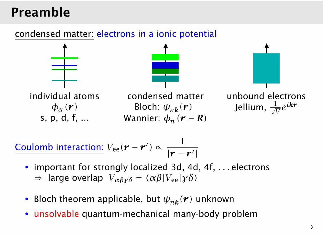
condensed matter: electrons in a ionic potential

individual atomsφα (r)

s, p, d, f, ...

condensed matterBloch: ψnk(r)

Wannier: φn (r −R)

unbound electrons

Jellium,1√Veikr

Coulomb interaction: Vee(r − r′)∝1

|r − r′|• important for strongly localized 3d, 4d, 4f, . . . electrons⇒ large overlap Vαβγδ = 〈αβ|Vee|γδ〉

• Bloch theorem applicable, but ψnk(r) unknown

• unsolvable quantum-mechanical many-body problem

3

Preamble



s, p, d, f, ...



unbound electrons

Jellium,1√Veikr





3

Density functional theory

Hohenberg & Kohn (’64):

E0 = E[ρ] = functional of electron density ρ(r)

= Ekin[ρ]+ Eion[ρ]+ EHartree[ρ]︸︷︷︸

known contributions

+ Exc[ρ]︸︷︷︸

unknown

Kohn & Sham (’65): ρ(r) =∑i |ϕi(r)|2

[− �2

2me∆+ Veff(r)

]ϕi(r) = εiϕi(r) Kohn-Sham equations

Veff(r) = Vion(r)+∫d3r ′ Vee(r−r′)ρ(r′)+

δExc[ρ]

δρ(r)

4





known contributions

+ Exc[ρ]︸︷︷︸

unknown

Kohn & Sham (’65): ρ(r) =∑i |ϕi(r)|2

[− �2

2me∆+ Veff(r)



δExc[ρ]

δρ(r)

4

Local Density Approximation

LDA: use Exc[ρ] of the homogeneous electron gas (ρ = const)

• solve Kohn-Sham equations by iteration

ρ(r) ⇒ Veff(r) ⇒ {εi, ϕi(r)} ⇒ ρ(r) ⇒ ...

• basis-dependent! (LMTO, [F]LAPW, ASW, ...)

very successful!

• advantages: provides bandstructure, intuitive one-particle picture

• problem: only certain part of Vee taken into account⇒ cannot describe strongly correlated systems

Hamilton-Operator:

HLDA =∑

ilm,jl′m′,σ

tilm,jl′m′ c+ilmσcjl′m′σ ( tilm,jl′m′ ↔ εklm )

5




ρ(r) ⇒ Veff(r) ⇒ {εi, ϕi(r)} ⇒ ρ(r) ⇒ ...


very successful!



Hamilton-Operator:

HLDA =∑

ilm,jl′m′,σ


5

Models for correlated electrons

interacting electrons: charge and spin degrees of freedom

H =∑

ijαβσ

tαβij c

+iασcjβσ +

∑

ijklαβγδσσ ′

Vαβγδijkl c+iασc

+jβσ ′clδσ ′ckγσ

⇒ metals, insulators, magnetism, superconductivity, ...

Hubbard model: e.g. 1 band, only

U = Viiii

HHubbard =∑

ijσ

tij c+iσcjσ + U

∑

i

ni↑ni↓

Heisenberg model: HHubbard

U�|tij|−→ HHeisenberg mit Jij =4t2ijU

HHeisenberg =∑

ij

Jij Si · Sj localized q.m. spins

6



H =∑

ijαβσ

tαβij c

+iασcjβσ +

∑






U = Viiii

HHubbard =∑

ijσ

tij c+iσcjσ + U

∑

i

ni↑ni↓



HHeisenberg =∑

ij


6



H =∑

ijαβσ

tαβij c

+iασcjβσ +

∑






U = Viiii

HHubbard =∑

ijσ

tij c+iσcjσ + U

∑

i

ni↑ni↓



HHeisenberg =∑

ij


6



H =∑

ijαβσ

tαβij c

+iασcjβσ +

∑






U = Viiii

HHubbard =∑

ijσ

tij c+iσcjσ + U

∑

i

ni↑ni↓



HHeisenberg =∑

ij


6



H =∑

ijαβσ

tαβij c

+iασcjβσ +

∑






U = Viiii

HHubbard =∑

ijσ

tij c+iσcjσ + U

∑

i

ni↑ni↓



HHeisenberg =∑

ij


6


limit of large coordination number Z or large dimension d:

• scaling: t = t? /√Z with Z ∝ d→ ∞

• Green function: Gij(ω)∝ d−||Ri−Rj ||/2

• self energy: Σij(ω) = δij Σ(ω) ⇒ local!

mapping onto single-site problem:

• self-energy Σii[Gii]⇒ same as for dynamical single-site problem

• e.g. Anderson impurity model ⇒ numerical methods!

⇒ Dynamical mean-field theory[Metzner & Vollhardt ’89; Müller-Hartmann ’89; Georges & Kotliar ’92; Georges et al. RMP ’96, ...]

7










7

LDA + DMFT

DMFT:

• exact for d = ∞• “thermodynamically consistent”, “conserving approximation”

• extensions: many bands, clusters, non-local interactions, ...

• impurity solvers: NRG, QMC, PQMC, ED, NCA... [→ lectures]

LDA+DMFT: [Anisimov et al. ’97; Lichtenstein & Katsnelson ’97; Liebsch & Lichtenstein ’00; Nekrasov et al. ’00; ...]

• use LDA band structure (as input, or self-consistently)

• on-site (“Hund’s rule”) interactions

• combine with DMFT, cluster extensions, ... [→ lectures]

8

LDA + DMFT

DMFT:








8

Part I

Introduction

1. Green functions

• Spectral representations

• Self-energy

• Path-integral formulation

2. Useful concepts

• Quasiparticles

• Hubbard bands

• Mott-Hubbard transition

9

1. Green functions

[e.g., Negele & Orland]

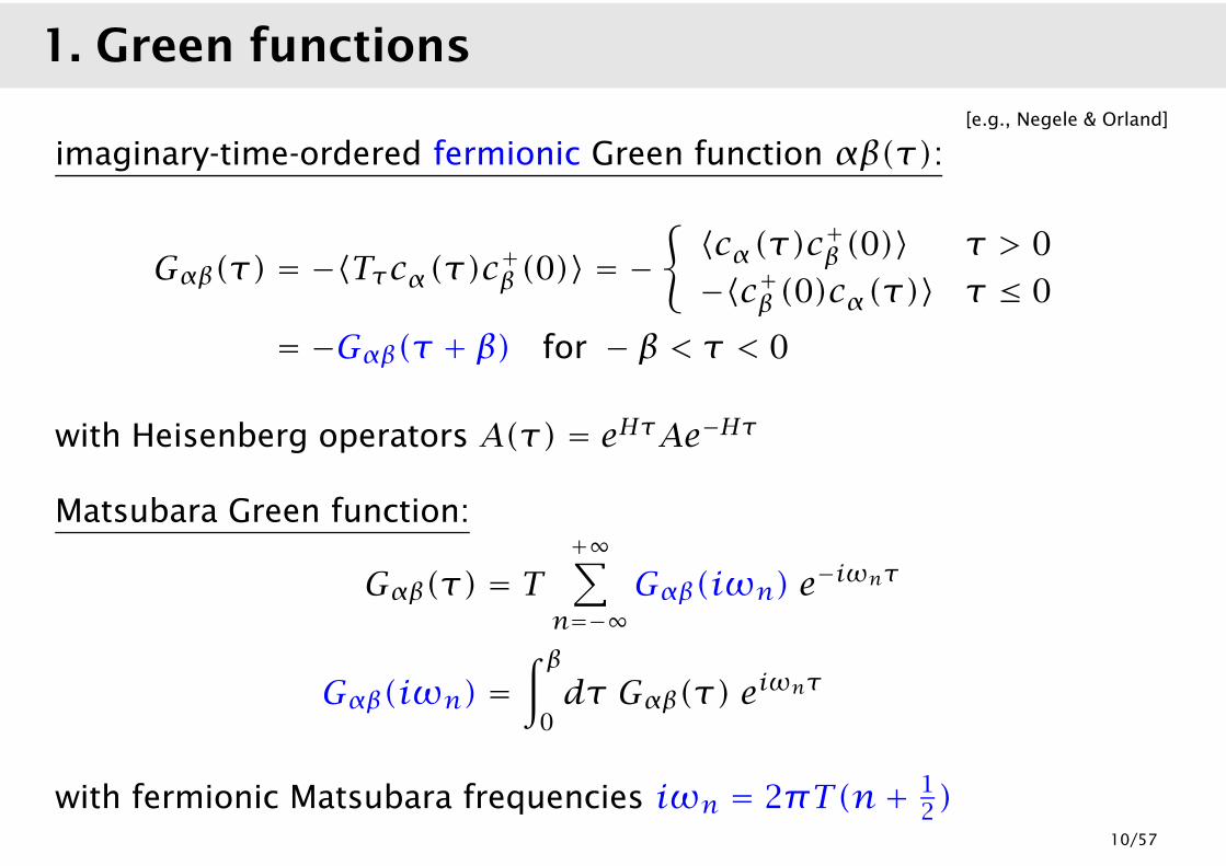
imaginary-time-ordered fermionic Green function αβ(τ):

Gαβ(τ) = −〈Tτcα(τ)c+β (0)〉 = −{〈cα(τ)c+β (0)〉 τ > 0

−〈c+β (0)cα(τ)〉 τ ≤ 0

= −Gαβ(τ + β) for − β < τ < 0

with Heisenberg operators A(τ) = eHτAe−Hτ

Matsubara Green function:

Gαβ(τ) = T+∞∑n=−∞

Gαβ(iωn) e−iωnτ

Gαβ(iωn) =∫ β

0dτ Gαβ(τ) e

iωnτ

with fermionic Matsubara frequencies iωn = 2πT(n+ 12)

10

1. Green functions




−〈c+β (0)cα(τ)〉 τ ≤ 0

= −Gαβ(τ + β) for − β < τ < 0



Gαβ(τ) = T+∞∑n=−∞


Gαβ(iωn) =∫ β

0dτ Gαβ(τ) e

iωnτ


10

Spectral representations

spectral function:

Gαβ(iωn) =∫∞−∞dω

Sαβ(ω)

iωn −ω

Sαβ(ω) = −1

πIm Gαβ(ω+ i0)︸︷︷︸

retarded Green function

= 1

Z

∑n,m

〈n|c+β |m〉〈m|cα |n〉 (e−βEm − e−βEn) δ(ω− (En − Em))

local Green function:

Giiσ (ω) = Gσ (ω) =1

L

∑

k

Gkσ (ω) (Imω≠0)

Siiσ (ω) = Sσ (ω) = −1

πIm

1

L

∑

k

Gkσ (ω+ i0)

= interacting density of states

11


spectral function:


Sαβ(ω)

iωn −ω

Sαβ(ω) = −1



= 1

Z

∑n,m




L

∑

k


Siiσ (ω) = Sσ (ω) = −1

πIm

1

L

∑

k

Gkσ (ω+ i0)

= interacting density of states11

Free particles

free particles: H − µN =∑

kσ

(εk − µ) c+kσckσ

⇒ G(0)kσ (ω) =1

ω+ µ − εk


Gσ (ω) =1

L

∑

k

1

ω+ µ − εk=∫∞−∞dε

ρ(ε)

ω+ µ − ε

Sσ (ω) =1

L

∑

k

δ(ω+ µ − εk) = ρ(ω+ µ)

with free density of states (which characterizes εk)

ρ(ω)=∑

k

δ(ω− εk)

12

Self-energy

self-energy Σk(ω):

Gkσ (ω)−1 = G(0)kσ (ω)−1 − Σkσ (ω) Dyson equation

Gkσ (ω) =1

ω+ µ − εk − Σkσ (ω)

matrix notation: Gijσ (iωn) = (G)ij,σ ,n

G−1 = G(0)−1 − ΣΣΣΣΣΣΣΣΣ

or G = G(0) +G(0)ΣΣΣΣΣΣΣΣΣG

diagrammatic notation:

= + Σ13

Path-integral formulation

partition function for fermionic Hamiltonian H({c+α}, {cα}) :

Z = Tre−β(H−µN) =∫

φα(β)=−φα(0)

D(φ∗α(τ),φα(τ)) exp(A)

= functional integral over Grassmann variables φα(τ)

action:

A = −∫ β

0dτ

[∑α

φ∗α (∂τ − µ)φα +H({φ∗α}, {φα})]


imaginary-time-ordered fermionic Green function:

Gαβ(τ) =1

Z

∫

APBC

D(φ∗φ) φα(τ)φ∗β(0) exp(A)

14




φα(β)=−φα(0)



action:

A = −∫ β

0dτ

[∑α

φ∗α (∂τ − µ)φα +H({φ∗α}, {φα})]



Gαβ(τ) =1

Z

∫

APBC


14

Part I

Introduction

1. Green functions


• Self-energy


2. Useful concepts

• Quasiparticles

• Hubbard bands


15

2. Useful concepts

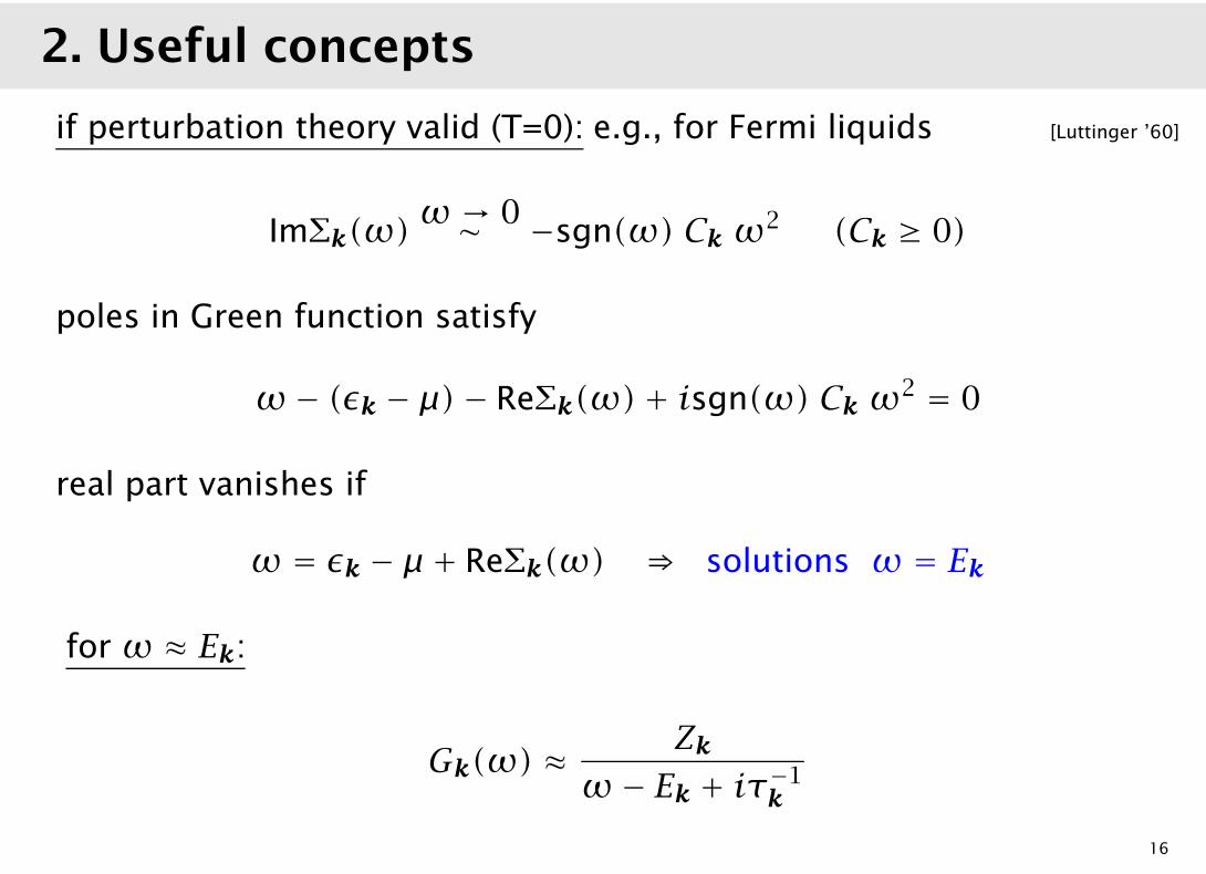
if perturbation theory valid (T=0): e.g., for Fermi liquids [Luttinger ’60]

ImΣk(ω)ω→ 0∼ −sgn(ω) Ck ω

2 (Ck ≥ 0)

poles in Green function satisfy

ω− (εk − µ)− ReΣk(ω)+ isgn(ω) Ck ω2 = 0

real part vanishes if

ω = εk − µ + ReΣk(ω) ⇒ solutions ω = Ek

for ω ≈ Ek:

Gk(ω) ≈Zk

ω− Ek + iτ−1k

16

2. Useful concepts



2 (Ck ≥ 0)





for ω ≈ Ek:

Gk(ω) ≈Zk

ω− Ek + iτ−1k

16

Quasiparticles

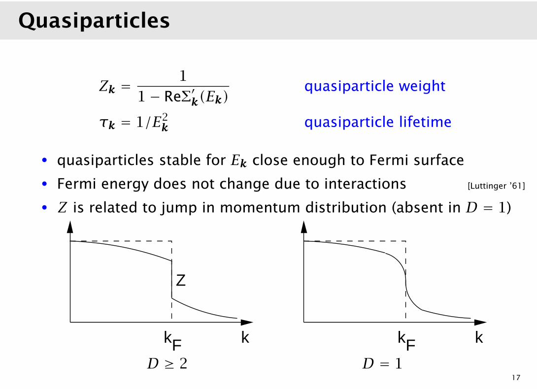
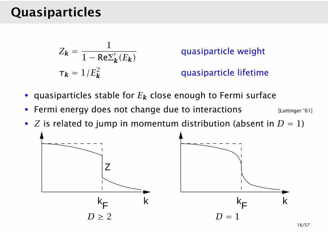
Zk =1

1− ReΣ′k(Ek)quasiparticle weight

τk = 1/E2k quasiparticle lifetime

• quasiparticles stable for Ek close enough to Fermi surface

• Fermi energy does not change due to interactions [Luttinger ’61]

• Z is related to jump in momentum distribution (absent in D = 1)

Z

kkF

n(k)

kkF

n(k)

D ≥ 2 D = 117

Hubbard bands, Mott transition

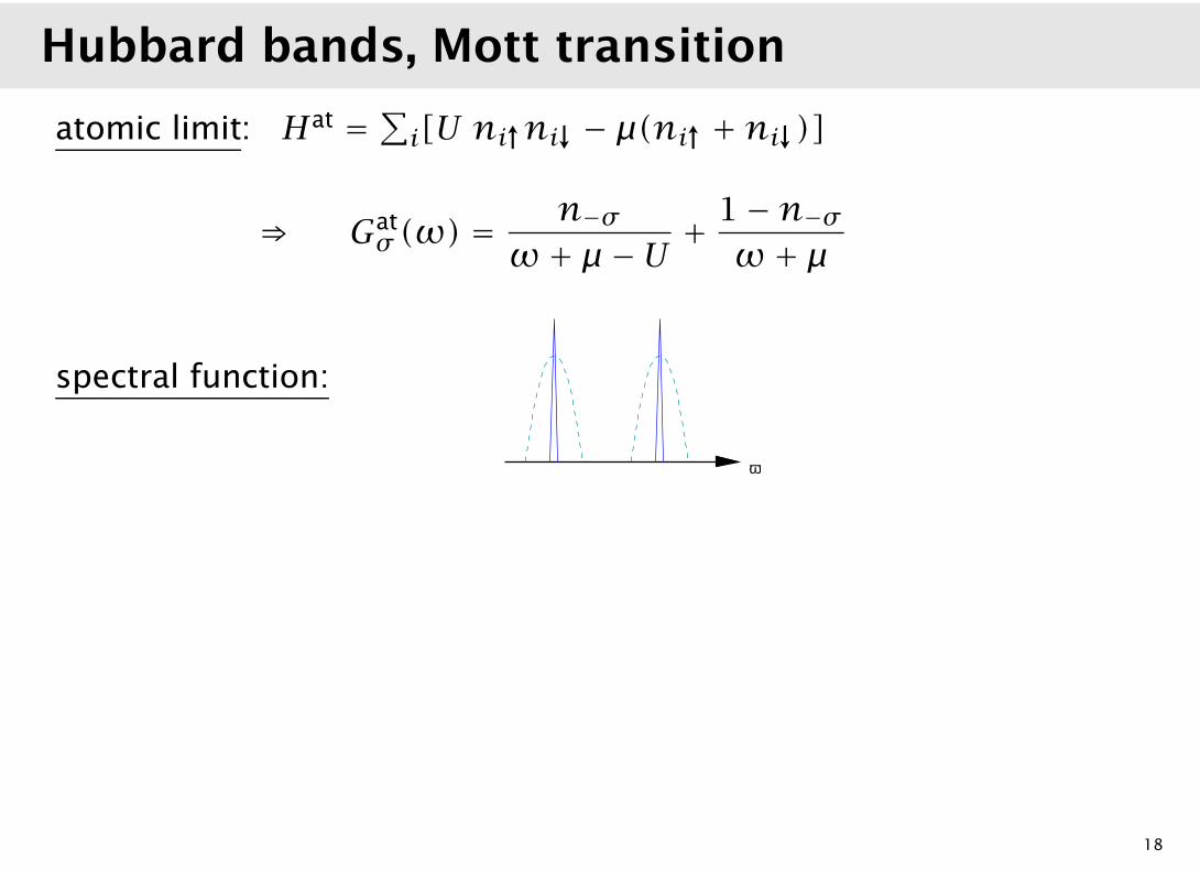
atomic limit: Hat =∑i[U ni↑ni↓ − µ(ni↑ +ni↓)]

⇒ Gatσ (ω) =

n−σω+ µ −U +

1−n−σω+ µ

spectral function:

ω

• peaks broaden for tij ≠ 0 ⇒ Hubbard bands [Hubbard ’63]

• Hubbard bands merge for large enough |tij|• quasiparticle bands develops gaps for large enough U

⇒ (non-magnetic) Mott-Hubbard transition at U = Uc and n = 1

[Mott ’46]

18



⇒ Gatσ (ω) =

n−σω+ µ −U +

1−n−σω+ µ

spectral function:

ω




[Mott ’46]

18

Part II

Fermions in infinite dimensions

1. Free fermions

• Scaling of hopping amplitudes

• Density of states

• Generalized lattices

2. Many-body theory

• Diagrammatic expansions

• Power-counting in 1/d

• Simplifications in d = ∞

19

1. Free fermions

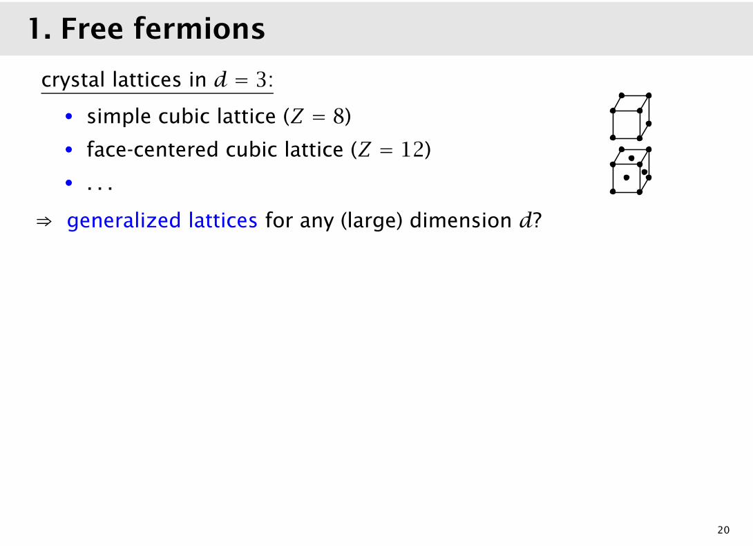
crystal lattices in d = 3:

• simple cubic lattice (Z = 8)

• face-centered cubic lattice (Z = 12)

• . . .

⇒ generalized lattices for any (large) dimension d?

easy for hypercubic lattice:

d = 1 d = 2 d = 3

in d dimensions:

e1 = (1,0,0, . . . )

e2 = (0,1,0, . . . )

. . . = . . .ed = (0,0,0, . . . ,1)

20

1. Free fermions




• . . .



d = 1 d = 2 d = 3

in d dimensions:

e1 = (1,0,0, . . . )

e2 = (0,1,0, . . . )

. . . = . . .ed = (0,0,0, . . . ,1)

20

Next-neighbor hopping

kinetic energy: Hkin =∑

ijσ

tij c+iσcjσ =

∑

kσ

εk c+kσckσ

NN hopping: tij = t(Ri −Rj) ={−t if Ri −Rj = ±en0 else

dispersion: εk = −2td∑

i=1

coski

nontrivial limit d → ∞?

density of states:

ρ(ε) = 1

L

∑

k

δ(ε− εk) L →∞=∫ddk

(2π)dδ(ε− εk)

21



ijσ

tij c+iσcjσ =

∑

kσ

εk c+kσckσ



i=1

coski


density of states:

ρ(ε) = 1

L

∑

k


(2π)dδ(ε− εk)

21

Scaling of hopping amplitudes

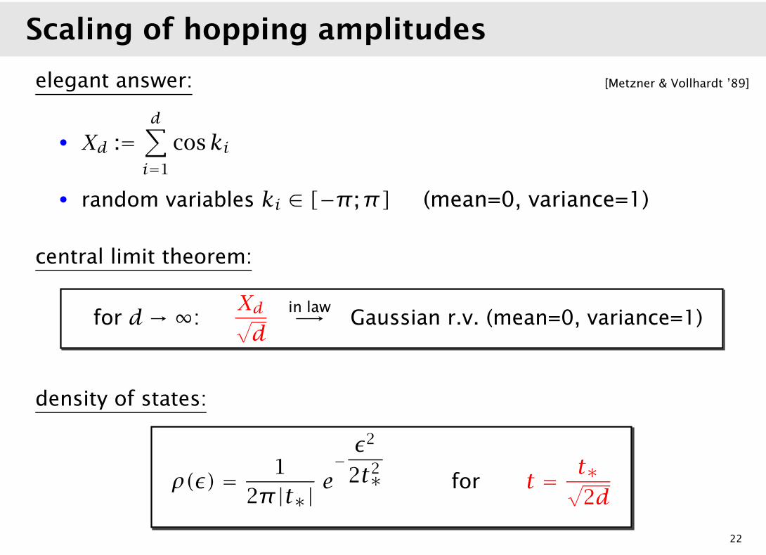
elegant answer: [Metzner & Vollhardt ’89]

• Xd :=d∑

i=1

coski

• random variables ki ∈ [−π ;π] (mean=0, variance=1)

central limit theorem:

for d→ ∞:Xd√d

in law−→ Gaussian r.v. (mean=0, variance=1)

density of states:

ρ(ε) = 1

2π|t∗|e−ε2

2t2∗ for t = t∗√2d

22



• Xd :=d∑

i=1

coski



for d→ ∞:Xd√d


density of states:

ρ(ε) = 1

2π|t∗|e−ε2

2t2∗ for t = t∗√2d

22

1/d corrections

Fourier transform: [Müller-Hartmann ’89]

Φ(s) =∫∞−∞dε eisε ρ(ε) =

∫ddk

(2π)deisεk factorizes!

=[∫ π

−π

dk

2πexp

(−2ist∗√

2dcosk

)]d= J0

(2t∗√2d

)d

=[

1− t2∗s

2

2d+O

(1

d

)]d= exp

[−t

2∗s

2

2+O

(1

d

)]

inverse transform:

ρ(ε) =∫∞−∞

dε

2πe−isε Φ(s)

= 1

2π|t∗|exp

[− ε

2

2t2∗+ 1

16d

(3− 6ε2

t2∗− 6ε4

t4∗

)+O

(1

d2

)]

23

1/d corrections



∫ddk


=[∫ π

−π

dk

2πexp

(−2ist∗√

2dcosk

)]d= J0

(2t∗√2d

)d

=[

1− t2∗s

2

2d+O

(1

d

)]d= exp

[−t

2∗s

2

2+O

(1

d

)]

inverse transform:

ρ(ε) =∫∞−∞

dε

2πe−isε Φ(s)

= 1

2π|t∗|exp

[− ε

2

2t2∗+ 1

16d

(3− 6ε2

t2∗− 6ε4

t4∗

)+O

(1

d2

)]

23

1/d corrections



∫ddk


=[∫ π

−π

dk

2πexp

(−2ist∗√

2dcosk

)]d= J0

(2t∗√2d

)d

=[

1− t2∗s

2

2d+O

(1

d

)]d= exp

[−t

2∗s

2

2+O

(1

d

)]

inverse transform:

ρ(ε) =∫∞−∞

dε

2πe−isε Φ(s)

= 1

2π|t∗|exp

[− ε

2

2t2∗+ 1

16d

(3− 6ε2

t2∗− 6ε4

t4∗

)+O

(1

d2

)]

23

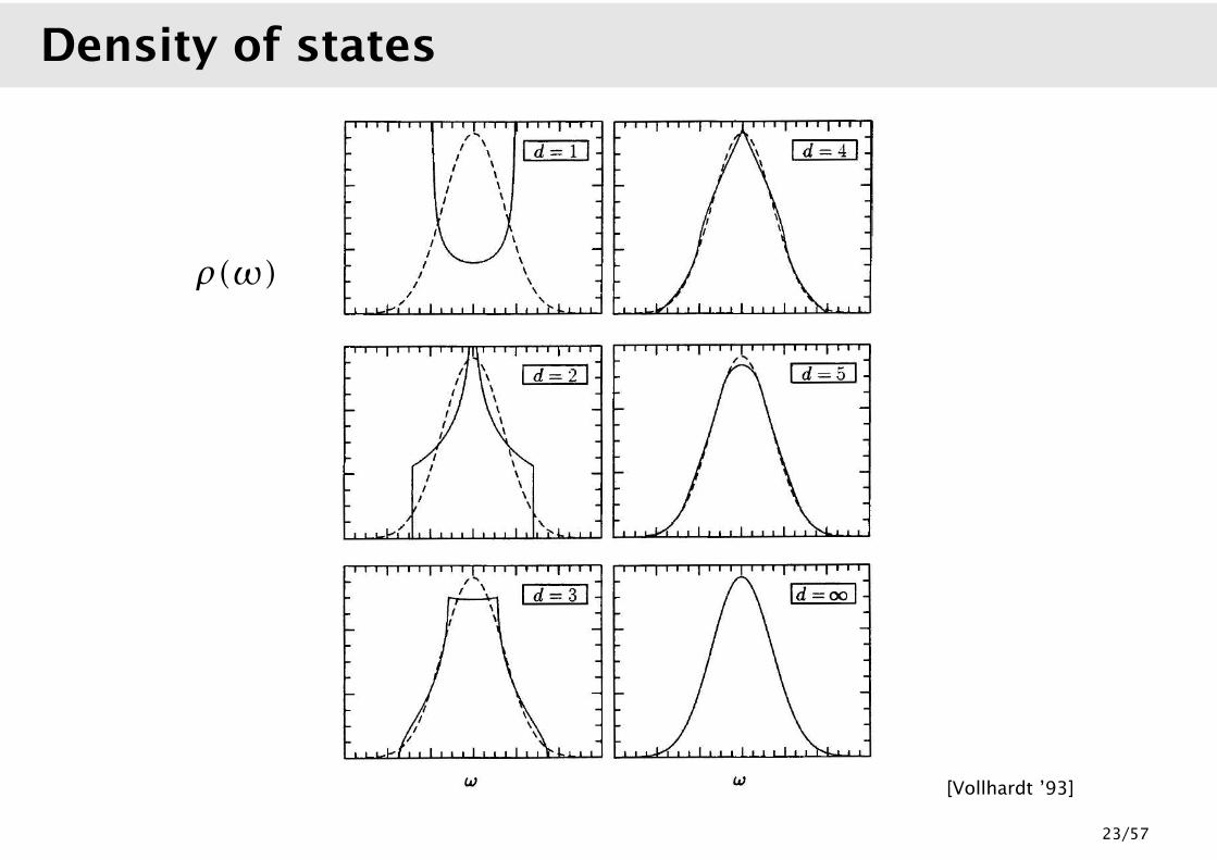
Density of states

ρ(ω)

[Vollhardt ’93]

24

Beyond nearest neighbors

[Müller-Hartmann ’89]

in general: tij ∝1√

# sites reached

hopping along axes: εaxesk =

∑

m≥1

(−2t(m)∗√

2d

)∑

i

cosmki

ρ(ε)∝ exp

(− ε2

2t2eff

)with teff =

√t(1)∗ + t(2)∗ + . . .

hopping to next-nearest neighbors: εNNNk ∼ t′

(∑

i

coski)2

ρ(ε)∝ cosh(E/a2) exp(−E2/2a2)

EE =

√1− 2aε+ a2, a =

√2t′∗t∗

25




# sites reached


∑

m≥1

(−2t(m)∗√

2d

)∑

i

cosmki

ρ(ε)∝ exp

(− ε2

2t2eff

)with teff =

√t(1)∗ + t(2)∗ + . . .


(∑

i

coski)2


EE =

√1− 2aε+ a2, a =

√2t′∗t∗

25

Density of states

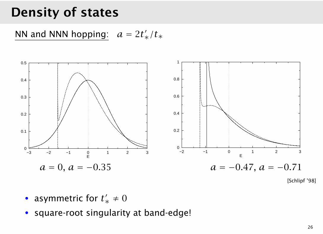
NN and NNN hopping: a = 2t′∗/t∗

0

0.1

0.2

0.3

0.4

0.5

−3 −2 −1 0 1 2 3

N∞0

E

0

0.2

0.4

0.6

0.8

1

−2 −1 0 1 2 3

N∞0

E

0

0.1

0.2

0.3

0.4

0.5

−3 −2 −1 0 1 2 3

N∞0

E

0

0.2

0.4

0.6

0.8

1

−2 −1 0 1 2 3

N∞0

E

a = 0, a = −0.35 a = −0.47, a = −0.71

[Schlipf ’98]

• asymmetric for t′∗ ≠ 0

• square-root singularity at band-edge!

26

Generalized fcc lattice

NN hoppingon fcc lattice

≡NNN hopping

on simple cubic lattice

ρ(ε)∝ e−(ε− εmin)/t∗√ε− εmin

for ε > εmin = −t∗√

2

• square-root singularity at band-edge

• small energy cost for spin-polarized states

⇒ favors ferromagnetism[Müller-Hartmann ’91;Ulmke ’98; Wahle et al. ’98, Vollhardt et al. ’99]

27

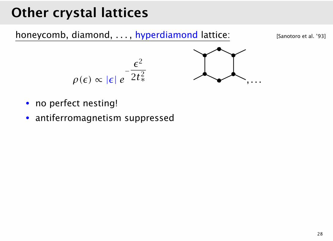
Other crystal lattices

honeycomb, diamond, . . . , hyperdiamond lattice: [Sanotoro et al. ’93]

ρ(ε)∝ |ε| e−ε2

2t2∗ , . . .

• no perfect nesting!

• antiferromagnetism suppressed

Lorentzian density of states: [Georges et al. ’96]

εk =t∗d

d∑

i=1

cot |ki| ⇒ ρ(ε) = 1

π

|t∗|t2∗ + ε2

• Ekin =∫ εF−∞dε ρ(ε) = ∞ ⇒ M.-I.-transition at Uc = ∞

28



ρ(ε)∝ |ε| e−ε2

2t2∗ , . . .




εk =t∗d

d∑

i=1

cot |ki| ⇒ ρ(ε) = 1

π

|t∗|t2∗ + ε2


28

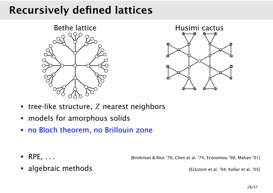
Recursively defined lattices

Bethe lattice Husimi cactus

��

��

��

��

��

��

��

��

��

��

!!!!"""""" ####

$$$$$$ %%%%&&&&&& ''''(((((((( ))))))

********* ++++,,,,,,,,, ----

...... ////000000 1111

222222 3333 444444 555566666666 777777

• tree-like structure, Z nearest neighbors

• models for amorphous solids

• no Bloch theorem, no Brillouin zone

• RPE, . . . [Brinkman & Rice ’70, Chen et al. ’74, Economou ’90, Mahan ’01]

• algebraic methods [Eckstein et al. ’04, Kollar et al. ’05]

29

Operator identities

hopping with d steps:

Hr =∑

dij=rc+i cj

H1 = NN hopping

Hr =Hr

(Z − 1)r/2, t∗r =

t∗r(Z − 1)r/2

d=2

d=3

operator identities for Bethe lattice:

H2 = (H1)2 − Z, . . . , ⇒

∞∑

r=0

Hr xr = 1− x2/(Z − 1)

1− xH1 + x2

• Hkin = ε(H1) ⇒ Hkin|λ〉 = ε(λ)|λ〉• ε(λ) = “dispersion” on interval −2 ≤ λ ≤ 2

30

Operator identities


Hr =∑

dij=rc+i cj

H1 = NN hopping

Hr =Hr

(Z − 1)r/2, t∗r =

t∗r(Z − 1)r/2

d=2

d=3


H2 = (H1)2 − Z, . . . , ⇒

∞∑

r=0

Hr xr = 1− x2/(Z − 1)

1− xH1 + x2


30

NN and NNN hopping

for NN hopping (Z = ∞):

ρ1(λ) =1

2π

√4− λ2

for any Hkin = ε(H1):

ρ(ε) =∫ 2

−2dλρ1(λ)δ(ε− ε(λ))

for NN and NNN hopping:

ε(λ) = const+ t∗1 λ+ t∗2 λ2

x = t∗2|t∗1 |+|t∗2 |

0

0.1

0.2

0.3

0.4

0.5

0.6

-2 -1 0 1 2 3

ρ t1∗ ,t 2∗ (

ε) t∗

ε / t∗

x = 0.00x = 0.05x = 0.10x = 0.15

0

0.2

0.4

0.6

0.8

1

-2 -1 0 1 2 3

ρ t1∗ ,t 2∗ (

ε) t∗

ε / t∗

x = 0.2x = 0.4x = 0.6x = 1.0

31

DOS for long-range hopping

t∗r ∝ exp(−const · d)

Hw =∑r w

r−1Hr

H+w =∑r w

r−1H2r

H−w =∑r w

r−1H2r−10

0.2

0.4

0.6

0.8

1

1.2

-2 -1 0 1 2 3 4

ρ w(ε

)

ε

w = 0.0w = 0.2w = 0.4w = 0.6

0

0.2

0.4

0.6

0.8

1

-3 -2 -1 0 1 2 3

ρ w+ (

ε)

ε

w= 0.0-0.3-0.6-0.9

0

0.1

0.2

0.3

0.4

0.5

0.6

0.7

0.8

-4 -3 -2 -1 0 1 2 3 4

ρ w- (ε)

ε

w= -0.4-0.6-0.8-1.0

32

Lattice representation of density of states

1-particle quantities:

• e.g., thermodynamics, Green function, . . .

• in d = ∞ only ρ(ε) enters (instead of εk)

• simply use ρ(ε) of finite-d system (e.g., LDA)

2-particle quantities, . . . :

• e.g., correlation functions, symmetry-broken phases, . . .

• need lattice with hopping amplitudes t∗r• any ρ(ε) can be represented for Z → ∞

ñ on hypercubic lattice [Blümer ’02]

ñ on Bethe lattice [Eckstein et al. ’04]

33











33

Part II


1. Free fermions




2. Many-body theory




34

2. Many-body theory

Feynman diagrams for Green functions:

= non-interacting Green function line G(0)

= interaction vertex

= full (interacting) Green function line G

perturbation expansion:

= + + + + + + . . .

35

Self-energy

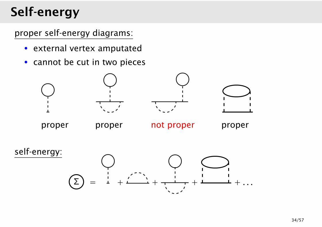
proper self-energy diagrams:

• external vertex amputated

• cannot be cut in two pieces

proper proper not proper proper

self-energy:

Σ = + + + + . . .

36

Skeleton expansion

so far: ΣΣΣΣΣΣΣΣΣ[G(0)]

now: omit self-energy insertions, etc.

⇒ skeleton expansion ΣΣΣΣΣΣΣΣΣ[G]

Σ = + + + . . .

• avoid double counting

• should be equivalent when summing all diagrams

• not equivalent when summing some diagrams

37

Power counting in 1/d

d dependence of Gijσ (ω) for d → ∞?

hopping amplitudes: tij = t∗ij d−12 ||Ri−Rj ||

kinetic energy:

Ekin,σ =∑

ij

tij〈c+iσcjσ 〉 = tij∫∞−∞

dω

2πiGijσ (ω) e

iω0+ = O(d0)

Green function:

Gijσ (ω) = O(d−12 ||Ri−Rj||) , Giiσ (ω) = O(d0)

⇒ simplifications for Feynman diagrams!

38




kinetic energy:

Ekin,σ =∑

ij

tij〈c+iσcjσ 〉 =∑

ij

tij

∫∞−∞

dω

2πiGijσ (ω) e

iω0+ = O(d0)

Green function:



38




kinetic energy:

Ekin,σ =∑

ij


ij︸︷︷︸O(d||Ri−Rj||)

tij

∫∞−∞

dω

2πiGijσ (ω) e

iω0+ = O(d0)

Green function:



38

Diagrammatic simplifications

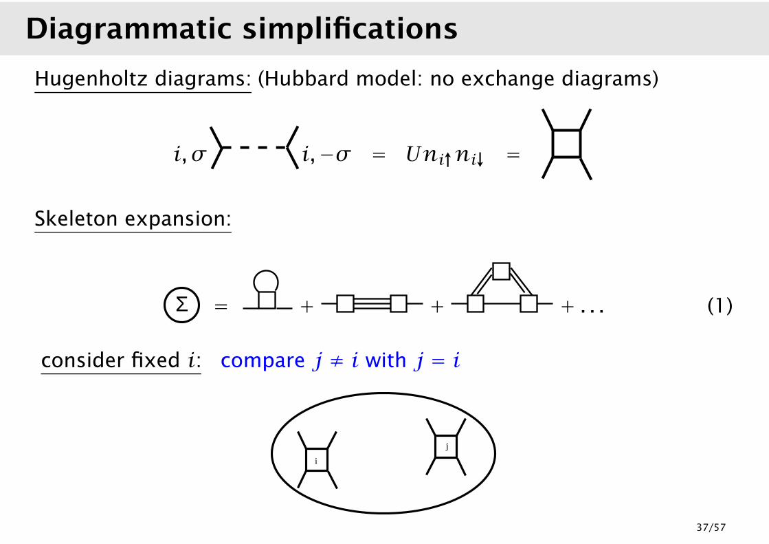
Hugenholtz diagrams: (Hubbard model: no exchange diagrams)

i, σ i,−σ = Uni↑ni↓ =

Skeleton expansion:

Σ = + + + . . . (0)

consider fixed i: compare j ≠ i with j = i

i

j

39

Collapse of position space diagrams

Skeleton expansion: ≥ 3 independent paths from i to j

• Green function lines: O(d−32 ||Ri−Rj ||)

• summation over j: O(d||Ri−Rj||)

⇒ skeleton diagram is O(d−12 ||Ri−Rj ||)

j

i

not skeleton

in d = ∞:

all vertices in ΣΣΣΣΣΣΣΣΣ[G] have the same site label!

self-energy is local!

Σijσ (ω) = δij Σiiσ (ω) = δij Σσ (ω)Σkσ (ω) = Σσ (ω) independent of k!

40






j

i

not skeleton

in d = ∞:




40






j

i

not skeleton

in d = ∞:




40

Consequences of local self-energy

• simple k dependence:

Gkσ (ω) =1

ω+ µ − εk − Σσ (ω)= G(0)kσ (ω− Σσ (ω))

• local Green function:

Gσ (ω) =∫ddk

(2π)d1

ω+ µ − εk − Σσ (ω)Dyson equation

=∫∞−∞dω

ρ(ε)

ω+ µ − Σσ (ω)− εHilbert transform

(later: “self-consistency equation”)

41

Pinning of DOS at Fermi surface

Volume of Fermi sea: unchanged by interactions [Luttinger ’60, ’61]

d = 3:

n = 2

∫ddk

(2π)dΘ(µ(0) − εk)

= 2

∫ddk

(2π)dΘ(µ − Σk(0)− εk)

shape of Fermisurface may change

d = ∞: shape unchanged, µ = µ(0) + Σ(0)

S(ω) = − 1

πIm

∫∞−∞dω

ρ(ε)

ω+ i0+ µ − Σσ (ω+ i0)− ε⇒ S(0) = ρ(µ(0))

spectral function is pinned at Fermi energy

[Müller-Hartmann 1989]

42



d = 3:

n = 2

∫ddk

(2π)dΘ(µ(0) − εk)

= 2

∫ddk

(2π)dΘ(µ − Σk(0)− εk)



S(ω) = − 1

πIm

∫∞−∞dω

ρ(ε)

ω+ i0+ µ − Σσ (ω+ i0)− ε⇒ S(0) = ρ(µ(0))



42

Non-local interactions

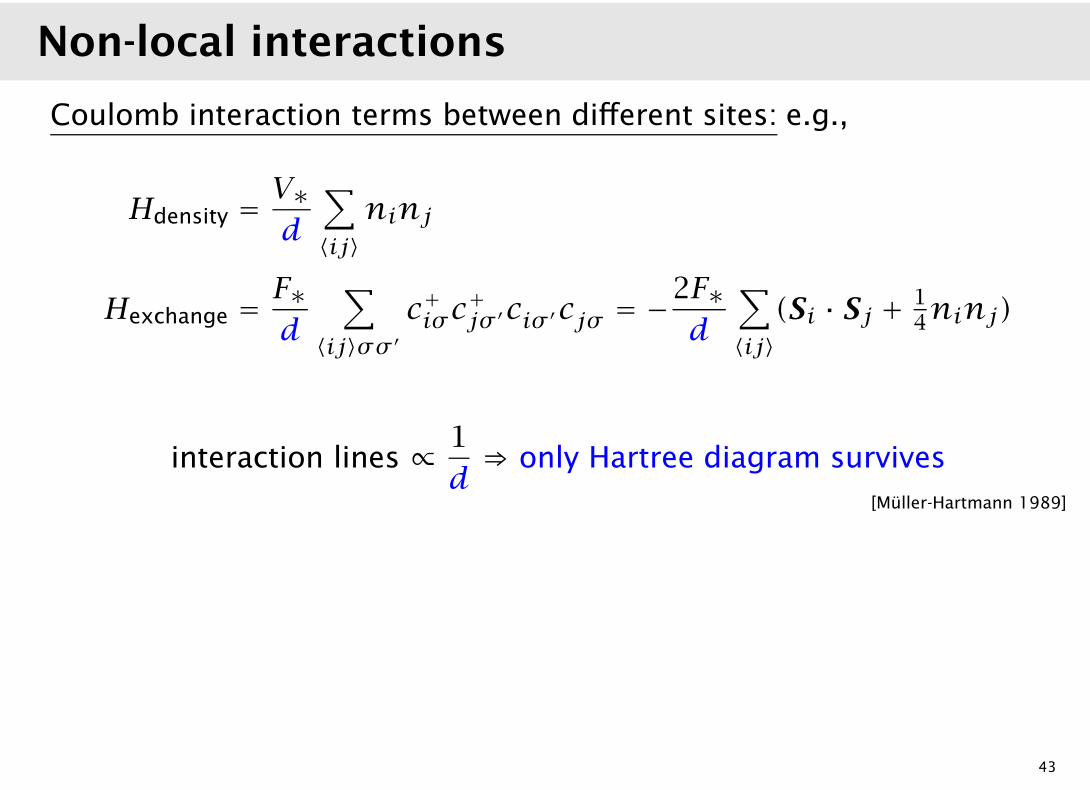
Coulomb interaction terms between different sites: e.g.,

Hdensity =V∗d

∑

〈ij〉ninj

Hexchange =F∗d

∑

〈ij〉σσ ′c+iσc

+jσ ′ciσ ′cjσ = −

2F∗d

∑

〈ij〉(Si · Sj + 1

4ninj)

interaction lines ∝ 1

d⇒ only Hartree diagram survives


“Extended DMFT”

• consider quantum fluctuations of Hdensity

• Hdensity − 〈Hdensity〉 = O(d−12 )

[Si et al. ’96,. . . ]

43



Hdensity =V∗d

∑

〈ij〉ninj

Hexchange =F∗d

∑



2F∗d

∑

〈ij〉(Si · Sj + 1

4ninj)




“Extended DMFT”



[Si et al. ’96,. . . ]

43

Part III


1. Mapping onto impurity models

2. A solvable example

3. Impurity solvers

4. Multi-band systems

44


Effective single-site action: A =A1 +A2 [Kotliar & Georges ’92, Jarrell ’92]

A1 =∫ β

0dτ

∫ β0dτ′

∑σ

c∗σ (τ)G−1σ (τ, τ

′) cσ (τ′)

=∑n,σ

c∗σ (iωn)Gσ(iωn)−1 cσ (iωn)

A2 = −U∫ β

0dτ c∗

↑(τ)c

↑(τ)c∗

↓(τ)c

↓(τ) local Hubbard interaction

Weiss field GGG: (GGG−1)τ,τ′ = G−1σ (τ, τ

′)

Green function: Gσ (iωn) = 〈cσ (iωn)c∗σ (iωn)〉A[GGG]

45



A1 =∫ β

0dτ

∫ β0dτ′

∑σ


′) cσ (τ′)

=∑n,σ


A2 = −U∫ β

0dτ c∗

↑(τ)c

↑(τ)c∗

↓(τ)c



′)


45

Dynamical mean field theory

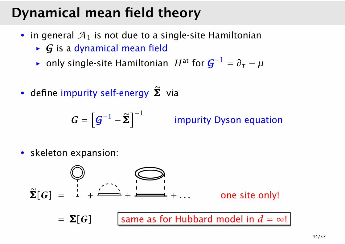
• in general A1 is not due to a single-site Hamiltonian

ñ GGG is a dynamical mean field

ñ only single-site Hamiltonian Hat for GGG−1 = ∂τ − µ

• define impurity self-energy ΣΣΣΣΣΣΣΣΣ via

G =[GGG−1 − ΣΣΣΣΣΣΣΣΣ

]−1impurity Dyson equation

• skeleton expansion:

ΣΣΣΣΣΣΣΣΣ[G] = + + + . . . one site only!

= ΣΣΣΣΣΣΣΣΣ[G] same as for Hubbard model in d = ∞!

46











46











46











46

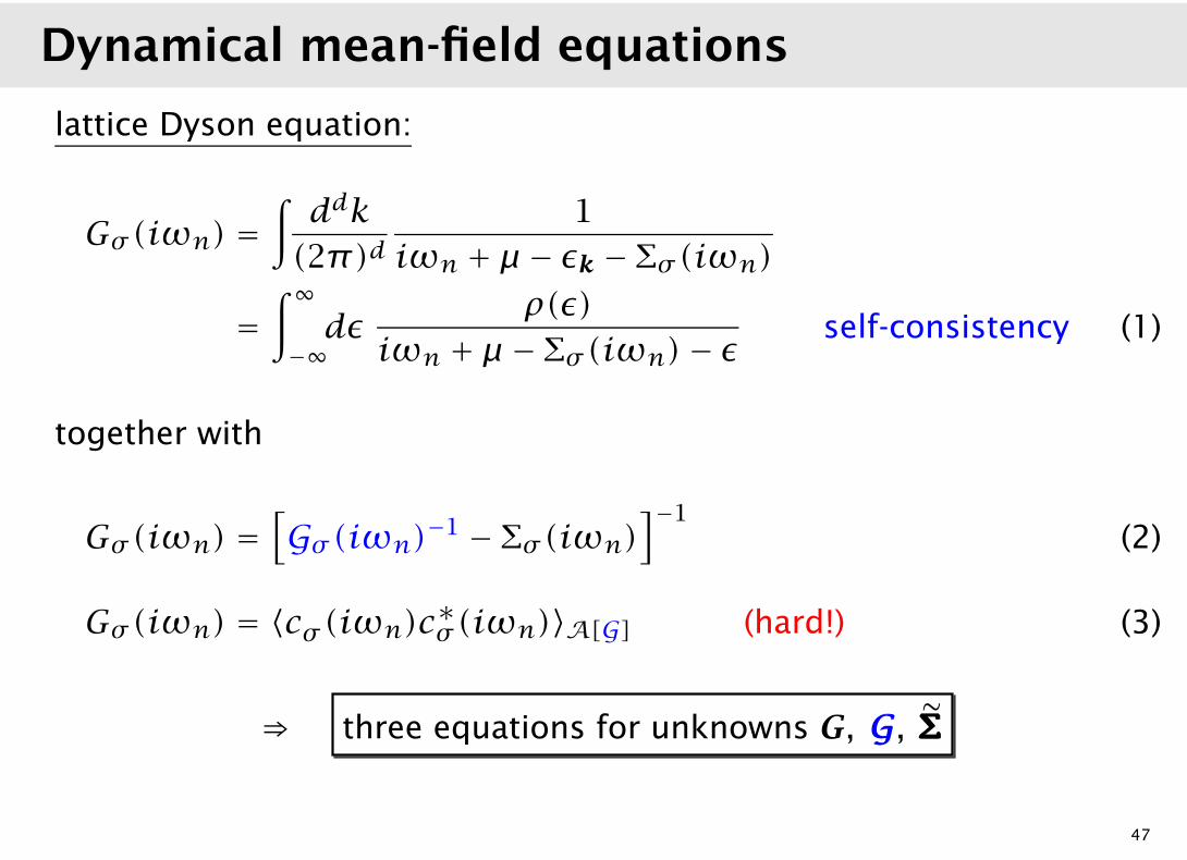
Dynamical mean-field equations

lattice Dyson equation:

Gσ (iωn) =∫ddk

(2π)d1

iωn + µ − εk − Σσ (iωn)

=∫∞−∞dε

ρ(ε)

iωn + µ − Σσ (iωn)− εself-consistency (1)

together with

Gσ (iωn)=[Gσ (iωn)−1 − Σσ (iωn)

]−1

Gσ (iωn)= 〈cσ (iωn)c∗σ (iωn)〉A[G] (hard!)

⇒ three equations for unknowns G, GGG, ΣΣΣΣΣΣΣΣΣ

47



Gσ (iωn) =∫ddk

(2π)d1


=∫∞−∞dε

ρ(ε)


together with

Gσ (iωn) =[Gσ (iωn)−1 − Σσ (iωn)

]−1(2)

Gσ (iωn) = 〈cσ (iωn)c∗σ (iωn)〉A[G] (hard!) (3)


47

Some simple limits

non-interacting case, U = 0: Σσ (iωn) = 0

(1)⇒ Gσ (iωn) = G(0)σ (iωn) = 1L

∑

k

G(0)k (iωn)

(2)⇒ Gσ (iωn) = Gσ (iωn) ⇒ (3) ✔

atomic limit, tij = 0, εk = 0: ρ(ε) = δ(ε)

(1)⇒ Gσ (iωn) =1

iωn + µ − Σσ (iωn)(2)⇒ Gσ (iωn)−1 = iωn + µ

⇒ G−1σ (τ) = ∂τ − µ ⇒ (3) ✔

48

Some simple limits


(1)⇒ Gσ (iωn) = G(0)σ (iωn) = 1L

∑

k

G(0)k (iωn)

(2)⇒ Gσ (iωn) = Gσ (iωn) ⇒ (3) ✔


(1)⇒ Gσ (iωn) =1


⇒ G−1σ (τ) = ∂τ − µ ⇒ (3) ✔

48


Falicov-Kimball model: hopping only for d spin species

H =∑

ij

tij d+i dj + Ef

∑

i

f+i fi +U∑

i

d+i di f+i fi

• d electrons hop on background of f electrons

• f configuration optimizes the free energy

• half-filling, bipartitie lattice, d ≥ 2:

checkerboard phase for U > 0 and T > Tc > 0 [Lieb ’86]

• DMFT exactly solvable [Brandt & Mielsch ’89, van Dongen ’90, Si et al. ’92, Freericks & Zlatic ’03]

49

DMFT equations

self-consistency for f electrons: G−1f = ∂τ − µ

DMFT action:

A =∫ β

0dτ

∫ β0dτ′d∗(τ)G−1

d (τ, τ′)d(τ′)

+∫ β

0dτf∗(τ)(∂τ − µ + Ef ) f (τ)−U

∫ β0dτ d∗(τ)d(τ)f∗(τ)f (τ)

integrate out f electrons: (atomic limit!)

Gd(iωn) = 〈d(iωn)d∗(iωn)〉A

= nfGd(iωn)−1 −U +

1−nfGd(iωn)−1

50

DMFT equations


DMFT action:

A =∫ β

0dτ


d (τ, τ′)d(τ′)

+∫ β

0dτf∗(τ)(∂τ − µ + Ef ) f (τ)−U





1−nfGd(iωn)−1

50

DMFT solution

self-consistency equations:

Gd(iωn) =∫∞−∞

dε ρd(ε)

iωn + µ − Σd(iωn)− ε

Gd(iωn)−1 = Gd(iωn)−1 − Σd(iωn)

⇒ determines Gd(iωn) for any density of states ρd(ε)

skeleton functional Σd[Gd]:

Σd(iωn) =U

2− 1

2Gd(iωn)±√√√(U

2− 1

2Gd(iωn)

)2

+ UnfGd(iωn)

involves all orders in U

51

DMFT solution


Gd(iωn) =∫∞−∞

dε ρd(ε)





Σd(iωn) =U

2− 1


2− 1

2Gd(iωn)

)2

+ UnfGd(iωn)


51

Spectral function of itinerant electrons

Bethe lattice, homogeneous phase, nd = nf = 12, U = 0.5, 1.0, . . . 3.0

[Freericks & Zlatic ’03]

• Mott metal-insulator transition at U = 2

• non-Fermi-liquid

• spectrum T independent in homogeneous phase52

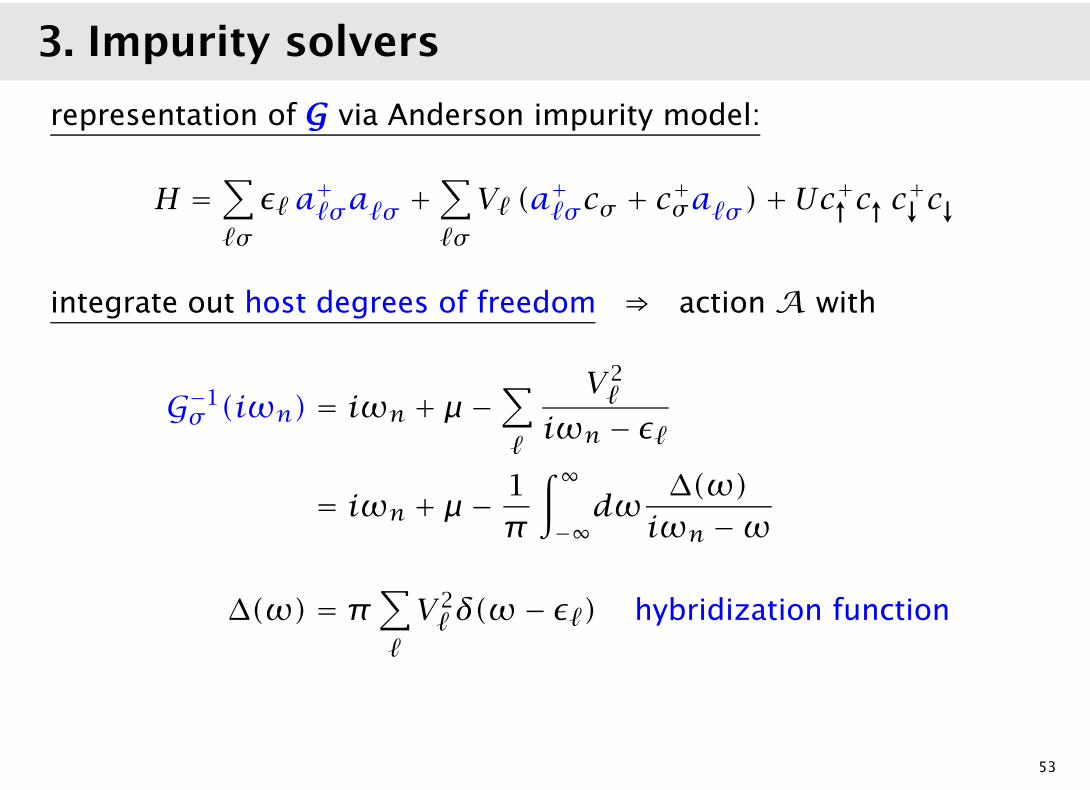
3. Impurity solvers

representation of GGG via Anderson impurity model:

H =∑

`σ

ε` a+`σa`σ +

∑

`σ

V` (a+`σcσ + c

+σa`σ )+Uc

+↑c↑c+↓c↓

integrate out host degrees of freedom ⇒ action A with

G−1σ (iωn) = iωn + µ −

∑

`

V2`

iωn − ε`

= iωn + µ −1

π

∫∞−∞dω

∆(ω)

iωn −ω

∆(ω) = π∑

`

V2`δ(ω− ε`) hybridization function

53

3. Impurity solvers


H =∑

`σ

ε` a+`σa`σ +

∑

`σ

V` (a+`σcσ + c

+σa`σ )+Uc

+↑c↑c+↓c↓



∑

`

V2`

iωn − ε`

= iωn + µ −1

π

∫∞−∞dω

∆(ω)

iωn −ω

∆(ω) = π∑

`


53

Numerical methods

QMC

Trotter decomposition of imaginary-time action, T not too small

PQMC

projection onto ground state, T = 0 only

NRG

logarithmic discretization of host spectrum, sites added successively

NCA

summation of a subset of Feynman diagrams

ED

exact diagonalization for small number of host sites

DMRG

blocks with varying number of sites, dynamical quantities available

[→ lectures]

54

Metal-insulator transition

Hubbard model, Bethe lattice, homogeneous phase, n = 1, DMFT(NRG)

−2.0 −1.0 0.0 1.0 2.0ω/W

0.0

0.5

1.0

1.5

A(ω

)*W

U/W=1.0U/W=1.42U/W=2.0

[Bulla ’99]

55

Phase diagram

Hubbard model, Bethe lattice, homogeneous phase, n = 1, DMFT(QMC)[Blümer ’02]

0

0.02

0.04

0.06

0.08

0.1

4.4 4.6 4.8 5 5.2 5.4 5.6 5.8

T

U

metal insulator

crossover region

critical end point

coexistenceregion

Uc1 Uc Uc2

• coexistence region [Uc1;Uc2], first-order transition

• crossover above critical region 56

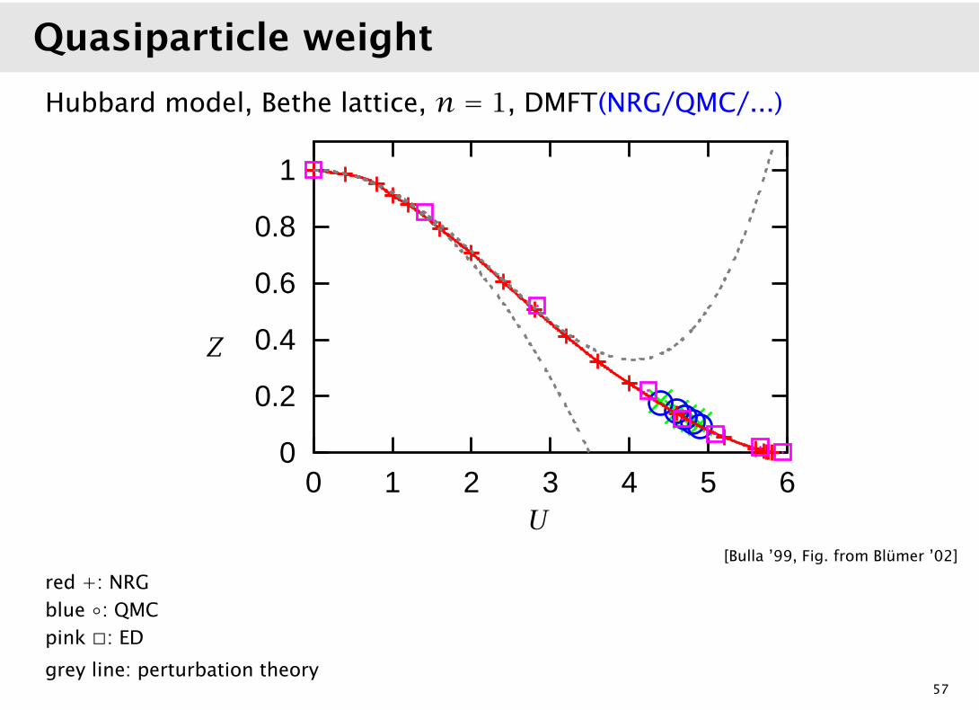
Quasiparticle weight

Hubbard model, Bethe lattice, n = 1, DMFT(NRG/QMC/...)

Z

0

0.05

0.1

0.15

0.2

0.25

4 4.5 5 5.5 6

Z

U

QMCQMC: 2π/(3γ)NRGED2nd/ 4th order

0

0.2

0.4

0.6

0.8

1

0 1 2 3 4 5 6

Z

UU[Bulla ’99, Fig. from Blümer ’02]

red +: NRG

blue ◦: QMC

pink �: ED

grey line: perturbation theory57

4. Multi-band systems: LDA+DMFT

LDA: Hartree-Term + ?

LDA+DMFT: include Coulomb interaction for correlated orbitals[Anisimov et al. ’97; Lichtenstein & Katsnelson ’97; Liebsch & Lichtenstein ’00; Nekrasov et al. ’00; ...]

Hint =1

2

∑

i=id,l=ld

∑

mσ,m′σ ′

′Uσσ

′mm′nilmσ nilm′σ ′

− 1

2

∑

i=id,l=ld

∑

mσ,m′

′Jmm′ c

†ilmσ c

†ilm′σ cilm′σ cilmσ

58




H = HLDA +Hint −HULDA

Hint =1

2

∑

i=id,l=ld

∑

mσ,m′σ ′

′Uσσ


− 1

2

∑

i=id,l=ld

∑

mσ,m′

′Jmm′ c

†ilmσ c


HULDA =already contained in LDA;determine from constrained LDA

58




H = HLDA +Hint −HULDA = H0LDA +Hint

Hint =1

2

∑

i=id,l=ld

∑

mσ,m′σ ′

′Uσσ


− 1

2

∑

i=id,l=ld

∑

mσ,m′

′Jmm′ c

†ilmσ c



H0LDA =

∑

ilm,jl′m′,σ

t0ilm,jl′m′ c+ilmσcjl′m′σ

58

Summary

DMFT:

• exact for d→ ∞• numerical solution of local dynamical many-body problem

• input: kinetic energy, interactions, band-filling (materials!)

• simplifications also for disordered systems

[→ lectures, talks]

Extensions: (numerical effort increases ...)

• multiband systems

• spatial fluctuations, clusters

• coupling to bosonic baths


59


Marcus Kollar

Theoretical Physics III, University of Augsburg, Germany

Summer School on

Dynamical Mean›Field Theory for Correlated Electrons:

Applications to Real Materials, Extensions and Perspectives

International Center for Theoretical Physics, Trieste

July 25 › August 3, 2005

1/57

Outline

Preamble

• Local-density approximation (LDA)

• Dynamical mean-field theory (DMFT)

• LDA + DMFT

I. Introduction

• Green functions

• Useful concepts

II. Fermions in infinite dimensions

• Free fermions

• Many-body theory

III. Dynamical mean-field theory

• Mapping onto impurity models

• A solvable example

• Impurity solvers

• Multiband systems

2/57

Preamble



s, p, d, f, ...



unbound electrons

Jellium,1√Veikr





3/57





known contributions

+ Exc[ρ]︸︷︷︸

unknown

Kohn & Sham (’65): ρ(r) =∑i |ϕi(r)|2

[− �2

2me∆+ Veff(r)



δExc[ρ]

δρ(r)

4/57




ρ(r) ⇒ Veff(r) ⇒ {εi, ϕi(r)} ⇒ ρ(r) ⇒ ...


very successful!



Hamilton-Operator:

HLDA =∑

ilm,jl′m′,σ


5/57



H =∑

ijαβσ

tαβij c

+iασcjβσ +

∑






U = Viiii

HHubbard =∑

ijσ

tij c+iσcjσ + U

∑

i

ni↑ni↓



HHeisenberg =∑

ij


6/57










7/57

LDA + DMFT

DMFT:








8/57

Part I

Introduction

1. Green functions


• Self-energy


2. Useful concepts

• Quasiparticles

• Hubbard bands


9/57

1. Green functions




−〈c+β (0)cα(τ)〉 τ ≤ 0

= −Gαβ(τ + β) for − β < τ < 0



Gαβ(τ) = T+∞∑n=−∞


Gαβ(iωn) =∫ β

0dτ Gαβ(τ) e

iωnτ


10/57


spectral function:


Sαβ(ω)

iωn −ω

Sαβ(ω) = −1



= 1

Z

∑n,m




L

∑

k


Siiσ (ω) = Sσ (ω) = −1

πIm

1

L

∑

k

Gkσ (ω+ i0)

= interacting density of states11/57

Free particles

free particles: H − µN =∑

kσ

(εk − µ) c+kσckσ

⇒ G(0)kσ (ω) =1

ω+ µ − εk


Gσ (ω) =1

L

∑

k

1

ω+ µ − εk=∫∞−∞dε

ρ(ε)

ω+ µ − ε

Sσ (ω) =1

L

∑

k

δ(ω+ µ − εk) = ρ(ω+ µ)

with free density of states (which characterizes εk)

ρ(ω)=∑

k

δ(ω− εk)

12/57

Self-energy

self-energy Σk(ω):

Gkσ (ω)−1 = G(0)kσ (ω)−1 − Σkσ (ω) Dyson equation

Gkσ (ω) =1

ω+ µ − εk − Σkσ (ω)

matrix notation: Gijσ (iωn) = (G)ij,σ ,n

G−1 = G(0)−1 − ΣΣΣΣΣΣΣΣΣ

or G = G(0) +G(0)ΣΣΣΣΣΣΣΣΣG

diagrammatic notation:

= + Σ13/57




φα(β)=−φα(0)



action:

A = −∫ β

0dτ

[∑α

φ∗α (∂τ − µ)φα +H({φ∗α}, {φα})]



Gαβ(τ) =1

Z

∫

APBC


14/57

2. Useful concepts



2 (Ck ≥ 0)





for ω ≈ Ek:

Gk(ω) ≈Zk

ω− Ek + iτ−1k

15/57

Quasiparticles

Zk =1

1− ReΣ′k(Ek)quasiparticle weight

τk = 1/E2k quasiparticle lifetime

• quasiparticles stable for Ek close enough to Fermi surface

• Fermi energy does not change due to interactions [Luttinger ’61]

• Z is related to jump in momentum distribution (absent in D = 1)

Z

kkF

n(k)

kkF

n(k)

D ≥ 2 D = 116/57



⇒ Gatσ (ω) =

n−σω+ µ −U +

1−n−σω+ µ

spectral function:

ω




[Mott ’46]

17/57

Part II


1. Free fermions




2. Many-body theory




18/57

1. Free fermions




• . . .



d = 1 d = 2 d = 3

in d dimensions:

e1 = (1,0,0, . . . )

e2 = (0,1,0, . . . )

. . . = . . .ed = (0,0,0, . . . ,1)

19/57



ijσ

tij c+iσcjσ =

∑

kσ

εk c+kσckσ



i=1

coski


density of states:

ρ(ε) = 1

L

∑

k


(2π)dδ(ε− εk)

20/57



• Xd :=d∑

i=1

coski



for d→ ∞:Xd√d


density of states:

ρ(ε) = 1

2π|t∗|e−ε2

2t2∗ for t = t∗√2d

21/57

1/d corrections



∫ddk


=[∫ π

−π

dk

2πexp

(−2ist∗√

2dcosk

)]d= J0

(2t∗√2d

)d

=[

1− t2∗s

2

2d+O

(1

d

)]d= exp

[−t

2∗s

2

2+O

(1

d

)]

inverse transform:

ρ(ε) =∫∞−∞

dε

2πe−isε Φ(s)

= 1

2π|t∗|exp

[− ε

2

2t2∗+ 1

16d

(3− 6ε2

t2∗− 6ε4

t4∗

)+O

(1

d2

)]

22/57

Density of states

ρ(ω)

[Vollhardt ’93]

23/57




# sites reached


∑

m≥1

(−2t(m)∗√

2d

)∑

i

cosmki

ρ(ε)∝ exp

(− ε2

2t2eff

)with teff =

√t(1)∗ + t(2)∗ + . . .


(∑

i

coski)2


EE =

√1− 2aε+ a2, a =

√2t′∗t∗

24/57

Density of states

NN and NNN hopping: a = 2t′∗/t∗

0

0.1

0.2

0.3

0.4

0.5

−3 −2 −1 0 1 2 3

N∞0

E

0

0.2

0.4

0.6

0.8

1

−2 −1 0 1 2 3

N∞0

E

0

0.1

0.2

0.3

0.4

0.5

−3 −2 −1 0 1 2 3

N∞0

E

0

0.2

0.4

0.6

0.8

1

−2 −1 0 1 2 3

N∞0

E

a = 0, a = −0.35 a = −0.47, a = −0.71

[Schlipf ’98]

• asymmetric for t′∗ ≠ 0

• square-root singularity at band-edge!

25/57

Generalized fcc lattice

NN hoppingon fcc lattice

≡NNN hopping

on simple cubic lattice

ρ(ε)∝ e−(ε− εmin)/t∗√ε− εmin

for ε > εmin = −t∗√

2

• square-root singularity at band-edge

• small energy cost for spin-polarized states

⇒ favors ferromagnetism[Müller-Hartmann ’91;Ulmke ’98; Wahle et al. ’98, Vollhardt et al. ’99]

26/57



ρ(ε)∝ |ε| e−ε2

2t2∗ , . . .




εk =t∗d

d∑

i=1

cot |ki| ⇒ ρ(ε) = 1

π

|t∗|t2∗ + ε2


27/57

Recursively defined lattices

Bethe lattice Husimi cactus

��

��

��

��

��

��

��

��

��

��

!!!!"""""" ####

$$$$$$ %%%%&&&&&& ''''(((((((( ))))))

********* ++++,,,,,,,,, ----

...... ////000000 1111

222222 3333 444444 555566666666 777777

• tree-like structure, Z nearest neighbors

• models for amorphous solids

• no Bloch theorem, no Brillouin zone

• RPE, . . . [Brinkman & Rice ’70, Chen et al. ’74, Economou ’90, Mahan ’01]

• algebraic methods [Eckstein et al. ’04, Kollar et al. ’05]

28/57

Operator identities


Hr =∑

dij=rc+i cj

H1 = NN hopping

Hr =Hr

(Z − 1)r/2, t∗r =

t∗r(Z − 1)r/2

d=2

d=3


H2 = (H1)2 − Z, . . . , ⇒

∞∑

r=0

Hr xr = 1− x2/(Z − 1)

1− xH1 + x2


29/57

NN and NNN hopping

for NN hopping (Z = ∞):

ρ1(λ) =1

2π

√4− λ2

for any Hkin = ε(H1):

ρ(ε) =∫ 2

−2dλρ1(λ)δ(ε− ε(λ))

for NN and NNN hopping:

ε(λ) = const+ t∗1 λ+ t∗2 λ2

x = t∗2|t∗1 |+|t∗2 |

0

0.1

0.2

0.3

0.4

0.5

0.6

-2 -1 0 1 2 3

ρ t1∗ ,t 2∗ (

ε) t∗

ε / t∗

x = 0.00x = 0.05x = 0.10x = 0.15

0

0.2

0.4

0.6

0.8

1

-2 -1 0 1 2 3

ρ t1∗ ,t 2∗ (

ε) t∗

ε / t∗

x = 0.2x = 0.4x = 0.6x = 1.0

30/57

DOS for long-range hopping

t∗r ∝ exp(−const · d)

Hw =∑r w

r−1Hr

H+w =∑r w

r−1H2r

H−w =∑r w

r−1H2r−10

0.2

0.4

0.6

0.8

1

1.2

-2 -1 0 1 2 3 4

ρ w(ε

)

ε

w = 0.0w = 0.2w = 0.4w = 0.6

0

0.2

0.4

0.6

0.8

1

-3 -2 -1 0 1 2 3

ρ w+ (

ε)

ε

w= 0.0-0.3-0.6-0.9

0

0.1

0.2

0.3

0.4

0.5

0.6

0.7

0.8

-4 -3 -2 -1 0 1 2 3 4

ρ w- (ε)

ε

w= -0.4-0.6-0.8-1.0

31/57











32/57

2. Many-body theory

Feynman diagrams for Green functions:

= non-interacting Green function line G(0)

= interaction vertex

= full (interacting) Green function line G

perturbation expansion:

= + + + + + + . . .

33/57

Self-energy

proper self-energy diagrams:

• external vertex amputated

• cannot be cut in two pieces

proper proper not proper proper

self-energy:

Σ = + + + + . . .

34/57

Skeleton expansion

so far: ΣΣΣΣΣΣΣΣΣ[G(0)]

now: omit self-energy insertions, etc.

⇒ skeleton expansion ΣΣΣΣΣΣΣΣΣ[G]

Σ = + + + . . .

• avoid double counting

• should be equivalent when summing all diagrams

• not equivalent when summing some diagrams

35/57




kinetic energy:

Ekin,σ =∑

ij


ij

∑

ij︸︷︷︸O(d||Ri−Rj ||)

tij

∫∞−∞

dω

2πiGijσ (ω) e

iω0+ = O(d0)

Green function:



36/57

Diagrammatic simplifications

Hugenholtz diagrams: (Hubbard model: no exchange diagrams)

i, σ i,−σ = Uni↑ni↓ =

Skeleton expansion:

Σ = + + + . . . (1)

consider fixed i: compare j ≠ i with j = i

i

j

37/57






j

i

not skeleton

in d = ∞:




38/57

Consequences of local self-energy

• simple k dependence:

Gkσ (ω) =1

ω+ µ − εk − Σσ (ω)= G(0)kσ (ω− Σσ (ω))

• local Green function:

Gσ (ω) =∫ddk

(2π)d1

ω+ µ − εk − Σσ (ω)Dyson equation

=∫∞−∞dω

ρ(ε)

ω+ µ − Σσ (ω)− εHilbert transform

(later: “self-consistency equation”)

39/57



d = 3:

n = 2

∫ddk

(2π)dΘ(µ(0) − εk)

= 2

∫ddk

(2π)dΘ(µ − Σk(0)− εk)



S(ω) = − 1

πIm

∫∞−∞dω

ρ(ε)

ω+ i0+ µ − Σσ (ω+ i0)− ε⇒ S(0) = ρ(µ(0))



40/57



Hdensity =V∗d

∑

〈ij〉ninj

Hexchange =F∗d

∑



2F∗d

∑

〈ij〉(Si · Sj + 1

4ninj)




“Extended DMFT”



[Si et al. ’96,. . . ]

41/57

Part III




3. Impurity solvers

4. Multi-band systems

42/57



A1 =∫ β

0dτ

∫ β0dτ′

∑σ


′) cσ (τ′)

=∑n,σ


A2 = −U∫ β

0dτ c∗

↑(τ)c

↑(τ)c∗

↓(τ)c



′)


43/57











44/57



Gσ (iωn) =∫ddk

(2π)d1


=∫∞−∞dε

ρ(ε)


together with

Gσ (iωn) =[Gσ (iωn)−1 − Σσ (iωn)

]−1(2)

Gσ (iωn) = 〈cσ (iωn)c∗σ (iωn)〉A[G] (hard!) (3)


45/57

Some simple limits


(1)⇒ Gσ (iωn) = G(0)σ (iωn) = 1L

∑

k

G(0)k (iωn)

(2)⇒ Gσ (iωn) = Gσ (iωn) ⇒ (3) ✔


(1)⇒ Gσ (iωn) =1


⇒ G−1σ (τ) = ∂τ − µ ⇒ (3) ✔

46/57


Falicov-Kimball model: hopping only for d spin species

H =∑

ij

tij d+i dj + Ef

∑

i

f+i fi +U∑

i

d+i di f+i fi

• d electrons hop on background of f electrons

• f configuration optimizes the free energy

• half-filling, bipartitie lattice, d ≥ 2:

checkerboard phase for U > 0 and T > Tc > 0 [Lieb ’86]

• DMFT exactly solvable [Brandt & Mielsch ’89, van Dongen ’90, Si et al. ’92, Freericks & Zlatic ’03]

47/57

DMFT equations


DMFT action:

A =∫ β

0dτ


d (τ, τ′)d(τ′)

+∫ β

0dτf∗(τ)(∂τ − µ + Ef ) f (τ)−U





1−nfGd(iωn)−1

48/57

DMFT solution


Gd(iωn) =∫∞−∞

dε ρd(ε)





Σd(iωn) =U

2− 1


2− 1

2Gd(iωn)

)2

+ UnfGd(iωn)


49/57

Spectral function of itinerant electrons

Bethe lattice, homogeneous phase, nd = nf = 12, U = 0.5, 1.0, . . . 3.0

[Freericks & Zlatic ’03]

• Mott metal-insulator transition at U = 2

• non-Fermi-liquid

• spectrum T independent in homogeneous phase50/57

3. Impurity solvers


H =∑

`σ

ε` a+`σa`σ +

∑

`σ

V` (a+`σcσ + c

+σa`σ )+Uc

+↑c↑c+↓c↓



∑

`

V2`

iωn − ε`

= iωn + µ −1

π

∫∞−∞dω

∆(ω)

iωn −ω

∆(ω) = π∑

`


51/57

Numerical methods

QMC

Trotter decomposition of imaginary-time action, T not too small

PQMC

projection onto ground state, T = 0 only

NRG

logarithmic discretization of host spectrum, sites added successively

NCA

summation of a subset of Feynman diagrams

ED

exact diagonalization for small number of host sites

DMRG

blocks with varying number of sites, dynamical quantities available

[→ lectures]

52/57

Metal-insulator transition

Hubbard model, Bethe lattice, homogeneous phase, n = 1, DMFT(NRG)

−2.0 −1.0 0.0 1.0 2.0ω/W

0.0

0.5

1.0

1.5

A(ω

)*W

U/W=1.0U/W=1.42U/W=2.0

[Bulla ’99]

53/57

Phase diagram

Hubbard model, Bethe lattice, homogeneous phase, n = 1, DMFT(QMC)[Blümer ’02]

0

0.02

0.04

0.06

0.08

0.1

4.4 4.6 4.8 5 5.2 5.4 5.6 5.8

T

U

metal insulator

crossover region

critical end point

coexistenceregion

Uc1 Uc Uc2

• coexistence region [Uc1;Uc2], first-order transition

• crossover above critical region 54/57

Quasiparticle weight

Hubbard model, Bethe lattice, n = 1, DMFT(NRG/QMC/...)

Z

0

0.05

0.1

0.15

0.2

0.25

4 4.5 5 5.5 6

Z

U

QMCQMC: 2π/(3γ)NRGED2nd/ 4th order

0

0.2

0.4

0.6

0.8

1

0 1 2 3 4 5 6

Z

UU[Bulla ’99, Fig. from Blümer ’02]

red +: NRG

blue ◦: QMC

pink �: ED

grey line: perturbation theory55/57




H = HLDA +Hint −HULDA = H0LDA +Hint

Hint =1

2

∑

i=id,l=ld

∑

mσ,m′σ ′

′Uσσ


− 1

2

∑

i=id,l=ld

∑

mσ,m′

′Jmm′ c

†ilmσ c



H0LDA =

∑

ilm,jl′m′,σ

t0ilm,jl′m′ c+ilmσcjl′m′σ

56/57

Summary

DMFT:

• exact for d→ ∞• numerical solution of local dynamical many-body problem

• input: kinetic energy, interactions, band-filling (materials!)

• simplifications also for disordered systems


Extensions: (numerical effort increases ...)

• multiband systems

• spatial fluctuations, clusters

• coupling to bosonic baths


57/57

Date post:	30-Aug-2020
Category:	Documents
Upload:	others
View:	3 times
Download:	0 times

Dynamical mean-field...

Documents