49
GeneticsOfPolygons.org Dynamical systems and Hamiltonian dynamics

An (autonomous) dynamical system is a set of parameters X which evolve in time
based on a well-defined set of rules.If this system is a pendulum or the planets in
our solar system, its evolution would typically be described by a set of differential
equations, so the evolution rules would be of the form: X'(t) = dX/dt = F(X(t)).
This is called a continuous-time system. If the system is discrete in nature, such as
the population of elk in Manitoba, the evolution rules would typically be difference
equations of the form X(n+1) = F(X(n)). Henri Poincare pioneered the idea of
using discrete mappings to study continuous systems and George Birkhoff of
Harvard advanced Poincare's ideas with the development of symbolic dynamics to
describe the evolution of a discrete system.
The ultimate goal of Dynamical Systems is to describe the evolution of X over
time. This would involve solving the differential equations or difference equations,
but if these equations are non-linear, it is unlikely that they can be solved
explicitly.
Instead of looking for a traditional 'time-series' solution X(t), an alternative is to
look for relationships between the variables that make up X. For example if X =
{x, dx/dt, y, dy/dt}, then a 'phase' plot of x vs dx/dt or y vs dy/dy might provide
valuable information. For example any closed curve in such a plot would imply
periodic behavior of that variable. If we were tracking the Earth's orbit and all of
the phase plots were periodic at the same time, the orbit itself would be periodic.
Below are examples of time series plots on top and corresponding phase plots on
bottom.
It is also valuable to find fixed points where the system might be approximated
locally by a linear system. For a continuous-time system, a fixed point X0 has the
form X0'(t) = 0. For a discrete-time system, a fixed point X0 has the form X0(n+1) =
X0(n).

Example: A continuous-time system
𝑋 = 𝑥𝑦 𝐹 𝑥
𝑦 = 𝑑𝑥 /𝑑𝑡
𝑑𝑦 /𝑑𝑡 = 𝑓₁ [x,y]
𝑓₂[𝑥 ,𝑦] = 𝑦+ 𝑥2+𝑦2 𝑥
− 𝑥+ 𝑥2+𝑦2 𝑦
The corresponding discrete-time system is
𝑋 = 𝑥𝑦 𝐹 𝑥
𝑦 = 𝑥(𝑛+1)
𝑦(𝑛+1) = 𝑓₁ [x,y]
𝑓₂[𝑥 ,𝑦] = 𝑦+ 𝑥2+𝑦2 𝑥
− 𝑥+ 𝑥2+𝑦2 𝑦
These are non-linear systems but the origin is a fixed point of both systems so the
Jacobian evaluated at the origin can be used to obtain a local linear system.
Definition: For a mapping 𝐹 𝑥𝑦 = 𝑓₁ [x,y]
𝑓₂[𝑥 ,𝑦] , the Jacobian is
JF =
𝜕𝑓₁
𝑑𝑥
𝜕𝑓₁
𝑑𝑦
𝜕𝑓₂
𝑑𝑥
𝜕𝑓₂
𝑑𝑦
For the systems given above the Jacobian is
D[F[{x, y}], {{x, y}}] = 3𝑥2 + 𝑦2 1 + 2𝑥𝑦
−1 + 2𝑥𝑦 𝑥2 + 3𝑦2 When x = 0 and y = 0, the
Jacobian is J= 0 1−1 0
. Eigenvalues[J] = {i,-i}, so the origin an elliptical fixed
point which is also called a 'center'. We can also see this from the vector flow lines
- which apply equally to the continuous or discrete case. The linearized system is
L[{x,y}]= {y,-x}and these vectors are tangent to circles centered at the origin as
shown below.

VectorPlot[L[{x,y}],{x,-1,1},{y,-1,1}] StreamPlot[L[{x,y}],{x,-1,1},{y,-1,1}]
We can trace the flow of the full system in the same way:
F[{x_,y_}]={y+(x^2+y^2)*x,-x+(x^2+y^2)*y}; StreamPlot[F[{x,y}],{x,-
2,2},{y,-2,2}]
This vector plot should make it clear that the non-linear system diverges in any
neighborhood of the origin - even thought the linear system appears to be 'stable'.
Below are the Mathematica simulations for the continuous case and the discrete
case.For the continuous case we can see that solutions rotate around the origin and
slowly diverge outwards.
2 1 0 1 2
2
1
0
1
2

solution=NDSolve[{x'[t]==y[t]+(x[t]^2 + y[t]^2)*x[t],y'[t]==-x[t]+(x[t]^2 +
y[t]^2)*y[t],x[0]==.05,y[0]==0},{x,y},{t,50}];
ParametricPlot[Evaluate[{x[t],y[t]}/.solution,{t,0,50}]]
In the discrete case we have similar behavior. The discrete linear map L[{x,y}]=
{y,-x} corresponds to a rotation by -Pi/2 so the full discrete map is a slowly
diverging form of this rotation as we can see below.
Plots=Flatten[Table[NestList[F,{x,0},300],{x, 0, .2,.005}],1];
Show[Graphics[{AbsolutePointSize[1.0],Point[Plots]},Axes-
>True,PlotRange{{left,right},{bottom,top}}]]

This example shows the difficulties that may arise with non-linear systems in the
neighborhood of a center. These issues would not exist if the fixed point were a
more predictable saddle point or sink or source. A center defines a very fine line
between stability and instability. Jurgen Moser used a discrete system very similar
to the one above to illustrate these problems:
Example: A discrete-time system (Section 34 from Lectures on Celestial
Mechanics by J.Moser and C.Siegel (1972))
𝑀 𝑥𝑦 =
𝑥+ 𝑦3 Cos A − ySin [A]
𝑥+ 𝑦3 Sin A + yCos [A]
This mapping is area preserving since the determinant is always 1. The origin is a
fixed point and the Jacobian at the origin is J = 𝐂𝐨𝐬[𝐀] −𝐒𝐢𝐧[𝐀]𝐒𝐢𝐧[𝐀] 𝑪𝒐𝒔[𝑨]
which is a
simple rotation by angle A. Sample plots are shown below
A = 1.111
M[{x_, y_}] := {(x + y^3)*Cos[A] - Sin[A]*y, (x+ y^3)*Sin[A] + Cos[A]*y};
Plots = Flatten[
Plots = Flatten[
Table[NestList[M, {x, 0}, 1000], {x, 0, .78535, .05178}], 1];
Show[Graphics[{AbsolutePointSize[1.0], Point[Plots]}, Axes -> True,
PlotRange -> {{-1.3, 1.3}, {-1.3, 1.3}}]]
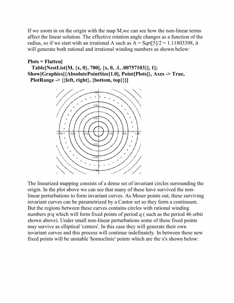
If we zoom in on the origin with the map M,we can see how the non-linear terms
affect the linear solution. The effective rotation angle changes as a function of the
radius, so if we start with an irrational A such as A = Sqrt[5]/2 = 1.11803398, it
will generate both rational and irrational winding numbers as shown below:
Plots = Flatten[
Table[NestList[M, {x, 0}, 700], {x, 0, .1, .00757103}], 1];
Show[Graphics[{AbsolutePointSize[1.0], Point[Plots]}, Axes -> True,
PlotRange -> {{left, right}, {bottom, top}}]]
The linearized mapping consists of a dense set of invariant circles surrounding the
origin. In the plot above we can see that many of these have survived the non-
linear perturbations to form invariant curves. As Moser points out, these surviving
invariant curves can be parametrized by a Cantor set so they form a continuum.
But the regions between these curves contains circles with rational winding
numbers p/q which will form fixed points of period q ( such as the period 46 orbit
shown above). Under small non-linear perturbations some of these fixed points
may survive as elliptical 'centers'. In this case they will generate their own
invariant curves and this process will continue indefinately. In between these new
fixed points will be unstable 'homoclinic' points which are the x's shown below:

Homoclinic points have local dynamics which are chaotic.No matter how small we
choose the neighborhood around the origin there will still be winding numbers that
are sufficient to form these fixed points which are guaranteed by the Birkhoff
Fixed Point Theorem. So at some level there will always be the potential for
chaotic behavior. This means that the ultimate stability issue is not related to the
size of the neighborhood, but rather to the nature of the non-linearities and how it
affects the invariant curves.
These are the issues addressed by the Twist Theorem. In Moser's words "instead of
expanding about the origin we need to expand near an unprturbed curve" and show
that it could survive.
Dynamics of Conservative Systems - the Hamiltonian
The law of Conservation of Energy says that for any physical process, the total
energy is unchanged with time, but for most systems it is almost impossible to
keep track of the flow of energy. A mechanical system like a car obeys this
principle but there is no practical way to determine the energy lost through heat
and friction. Satellites in earth orbit have very low 'resistance' due to the thin
atmosphere, but eventually they lose energy to heat and friction. In the depths of
space it is much easier to balance the energy equation. When formulating the laws
of motion of the planets it is safe to ignore friction or 'damping' because the
surrounding space is nearly a vacuum and the bodies are large. The complications
which arise in celestial mechanics involves the gravitational interaction of the
planets. This is where resonances can play a major role.
Five orbits of Jupiter take almost the same time as two of Saturn, so these two
giants have an almost 5:2 resonance. This would be classified as a major resonance
- especially when it involves two gas giants. No one knows how this will play out
over long time periods because there are other planets involved. Most scientists

agree that the gas giants were formed early on the life of the solar system at a much
closer distance to the sun that we see now. (Along these lines the drawing below is
a schematic and is not to scale.)
Working backwards to the early solar system, it now seems likely that Jupiter and
Saturn once shared an even more dangerous 2:1 resonance when they were in
orbits much closer to the sun. The highly regarded Nice model of the early solar
system, which was released in 2005, includes a simulation which shows how this
resonance could scatter the four gas giants - ejecting Neptune and Uranus to the
outer disk which was filled with small planetesimals. The model has many features
that match current theories, for example it explains the 'late heavy bombardment'
which was a time when the Earth and Moon were bombarded by meteorites. These
could well have been the meteorites which were scattered when Neptune and
Uranus appeared in the thick ring of planetesimals.
Shown above is a 'chaotic' orbit of a smaller mass which is interacting with two
larger bodies. This could be an asteroid under the influence of the sun and Jupiter.
The first person to realize that unpredictable chaotic orbits could exist for three or
more bodies was Henri Poincare (1854-1912). Here is a quote from his essay on
Science and Method
"It may happen that small differences in the initial conditions produce very great
changes in the final phenomena. A small error in the former will produce an
enormous error in the latter. Prediction becomes impossible."
This phenomena is called 'sensitive dependence on initial conditions (sic)' and it is
very real. Even with super computers and very high precision, some calculations
are fruitless because small initial errors (which always exist) will eventually yield
large errors.

There is no universally acceptable definition of chaotic behavior but everyone
agrees that the most important ingredient is the sic condition because it puts a
practical limit on what we can expect to achieve. At the 1986 international
conference on chaos held by the Royal Society in London, the following definition
was put forward:
"Chaotic behavior is stochastic behavior in a deterministic system."
Stochastic behavior means the behavior is random and therefore as unpredictable
as a coin toss. This definition is consistent with the SIC criteria. Jurgen Moser's
textbook on the subject was based on his 1972 lectures at the Institute for
Advanced Studies at Princeton. It was called "Stable and Random Motions in
Dynamical Systems"
The modern formulation of the equations of motion of the planets is in terms of the
Hamiltonian which represents the total energy of the system. The Hamiltonian is
essentially the sum of the Kinetic Energy and Potential energy. Below is an
example of how the Hamiltonian can be used to formulate and analyze the motion
of an pendulum where we temporarily ignore frictional effects.This Ideal
Pendulum conserves energy, so we can use the Hamiltonian to derive the equations
for motion.
Hamiltonian Dynamics
The Hamiltonian of a physical system is a function of (generalized) position q
,
and (generalized) momentum p
. In some cases it may change in time, so it is
writen as ( ( ), ( ), )i iH q t p t t where i = 1,....N are the degrees of freedom of the
physical system. The dynamics of a Hamiltonian system are given by:
, i i
i i
H Hq p
p q
So a Hamiltonian system is a system of differential equations which are related by
H. Not every system of differential equations has a corresponding Hamiltonian.
When H does not depend explicitly on time, the state of the system at any given
time is a point (pi,qi) in 2N-dimensional space phase space. The motion of this
point is determined by the equations above. Starting with an initial set of points,
the volume will be preserved over time because the equations above imply that H
is conserved: 0i i
i i
dp dqdH H H
dt p dt q dt

When N = 2, there are two position coordinates q
={q1,q2} and two momentum
coordinates p
= {q1,q2} so the system is 4-dimensional. For example if the
differential equations describe the motion of 2 planets around the sun, then the
system motion would be periodic in {q1,p1} and {q2,p2} so there would be two
frequencies. The Hamiltonian would not be constant, but it would be periodic so
these two phase plots would combine together to yield motion on a 2-torus
Below is the case of a 2-year period vs a 5-year period which is similar to Saturn
(29.447 years) and Jupiter (11.861 years), so 5*11.861 ≈ 2*29.447. This is called a
'rational' torus. If the periods were incommensurable, like Earth and Jupiter, the
windings would fill the torus and it would be called an irrational torus. The
corresponding motion is called a quasi-periodic orbit. These are the most stable
orbits because the gravitational interactions have no 'resonances'.
gr1=ParametricPlot3D[{(2+Cos[u])*Cos[v],(2+Cos[u])*Sin[v],Sin[u]},{v,0,2*P
i},{u,0,2*Pi},
Mesh->False, Boxed->False, Axes->False]; (*this is the solid torus with radii 2
and 1*)
gr2=ParametricPlot3D[{(2+Cos[5 t]) Cos[2 t],(2+Cos[5 t]) Sin[2 t],Sin[5
t]},{t,0,2 Pi}];
Show[gr1,gr2]
To reduce this motion to a 2-dimensional mapping, choose a reference plane, for
example slice the torus at a fixed longitude q0 and 'strobe' the longer 5 year period
with the shorter 2-year period by setting δt = 2 years. This would yield a map S
with a periodic orbit with 5 dots as shown above.
These surfaces of section are also called Poincare return maps. They can be used to
help uncover periodic motion or fixed points.Since the system equations are
differential equations, continuity would imply that orbits in the vicinity of a fixed
point will behave in a predictable fashion based on the Jacobian. Because S is

symplectic, the Jacobian at any fixed point will have eigenvalues of the form {λ,
1/λ). There are only three types of behavior possible near a fixed point:
(i) λ positive and λ > 1 (1/λ < 1) This is an unstable hyperbolic 'saddle' point
where the motion expands in one diretion and contracts in another.
(ii) λ negative and |λ| >1, (1/|λ| <1). Similar to (i) above but displacements in each
direction vary from positive to negative on each iteration.
(iii) λ complex - in which case λ and 1/λ must have zero real part so they have the
form λ = eiθ and 1/λ = e
-iθ. This is called a 'center' or a neutral fixed point. Nearby
points will rotate by θ on each iteration.
Case (iii) is the only case where stability is not obvious, because this 'marginally
stable' behavior may be very sensiitive to small perturbations. This is the heart of
the KAM Theorem: How will the marginally stable fixed points of a 'well-behaved'
Hamiltonian system react when subjected to periodic perturbations ? (i.e. when
gravity between Jupiter and Saturn is turned on). Will a finite measure of the quasi-
periodic orbits survive ? Is the solar system stable ?
Note that it is not possible for solutions to spiral into or away from a fixed point
and also it is not possible to have expansion without contraction. These are
consequences of the symplectic property of the Hamiltonian.
A 2-degree of freedom Hamiltonian such as the one above would be classified as
'well-behaved' or integrable, if there are 2 integrals of motion. A function f( p
, q
) is
an Integrable of Motion if it satisfies the 'Poisson bracket' (commutator)
relationship.
[f, H] = 0i i
i i
p qf f df
p t q t dt
Therefore an integral of motion is also a constant of motion. The system energy H(
p
, q
) is always a constant of motion. Note that the torus maps shown above have
non-Eulidean metric, just like the raw Df maps. We can obtain the integrals of
motion by performing a canonical change of variables to convert the map S into
'normal' Euclidean form so that ellipses become circles. The new variables are
called 'action-angle' variables: ( p
, q
) → ( , )I
.In the new surface of section map,
θ will represent a simple rotation. The I's are the two constants of motion:
.
j
j
C
I p dq
where the integral is around the jth axis of the torus.
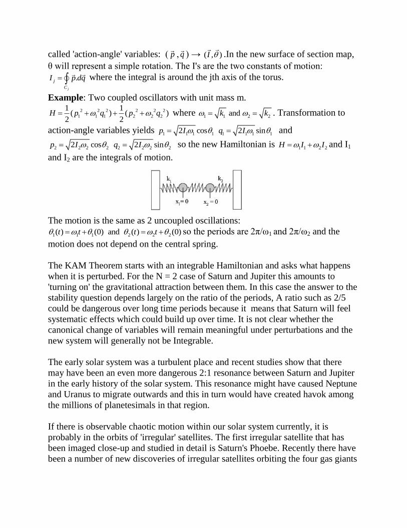
Example: Two coupled oscillators with unit mass m.
2 2 2 2 2 2
1 1 1 2 2 2
1 1( ) ( )
2 2H p q p q where 1 1 2 2 and k k . Transformation to
action-angle variables yields 1 1 1 1 1 1 1 12 cos 2 sin p I q I and
2 2 2 2 2 2 2 22 cos 2 sin p I q I so the new Hamiltonian is 1 1 2 2H I I and I1
and I2 are the integrals of motion.
The motion is the same as 2 uncoupled oscillations:
1 1 1 2 2 2( ) (0) and ( ) (0)t t t t so the periods are 2π/ω1 and 2π/ω2 and the
motion does not depend on the central spring.
The KAM Theorem starts with an integrable Hamiltonian and asks what happens
when it is perturbed. For the N = 2 case of Saturn and Jupiter this amounts to
'turning on' the gravitational attraction between them. In this case the answer to the
stability question depends largely on the ratio of the periods, A ratio such as 2/5
could be dangerous over long time periods because it means that Saturn will feel
systematic effects which could build up over time. It is not clear whether the
canonical change of variables will remain meaningful under perturbations and the
new system will generally not be Integrable.
The early solar system was a turbulent place and recent studies show that there
may have been an even more dangerous 2:1 resonance between Saturn and Jupiter
in the early history of the solar system. This resonance might have caused Neptune
and Uranus to migrate outwards and this in turn would have created havok among
the millions of planetesimals in that region.
If there is observable chaotic motion within our solar system currently, it is
probably in the orbits of 'irregular' satellites. The first irregular satellite that has
been imaged close-up and studied in detail is Saturn's Phoebe. Recently there have
been a number of new discoveries of irregular satellites orbiting the four gas giants

Jupiter, Saturn, Uranus and Neptune. These discoveries were made posible by
attaching new wide-field CCD cameras to large telescopes.
The Earth recently captured a small irregular asteriod. It was called 2006 RH120
and it was about 15 meters wide. It only survived for about 4 orbits before
returning to its orbit around the sun. The dates were September 2006 to June 2007.
Latest news is that there is another companion to the Earth in an irregular orbit. It
is known as 2010 SO16.
The Hamiltonian Equations for an Ideal Pendulum:
Definition: A system of differential equations
𝐹 𝑥𝑦 = 𝑥′
𝑦′ = 𝑓 [x,y]
𝑔[𝑥 ,𝑦] is a Hamiltonian system if there is a real-valued
function H[{x,y}] such that for all {x,y}:
𝜕𝐻
𝜕𝑦 = f[x,y] and
𝜕𝐻
𝜕𝑥 = -g[x,y]
For conservative systems H will always represent the (constant) total energy of the
system, so we can sometimes start with H = Kinetic Energy + Potential Energy and
use this to derive the system equations.
Gravitational potential energy for an object on the Earth's surface is V = mgh
where m is the mass of the object (say in kilograms) , g is the force of gravity
(about 9.81 kg/sec2) and h is the height (in meters).
There is no universal standard for choosing height, so two people might find
different values for V. This is usually not an issue because it just means they will
have a value for total energy H which differs by this same constant. We will
measure height relative to the support point (h = 0) as shown in the diagram. This
means that the bob will have negative V when it is below the h = 0 line and
positive V above.
The simple pendulum has only two variables, the angular displacement θ and the
'velocity' dθ/dt' which we will abbreviate θ'.
When the pendulum is raised upwards by an angle θ as shown here, its height is
increased from -L to -LCos[θ], so this increases the potential energy of the
system. The general equation for the Potential Energy is:
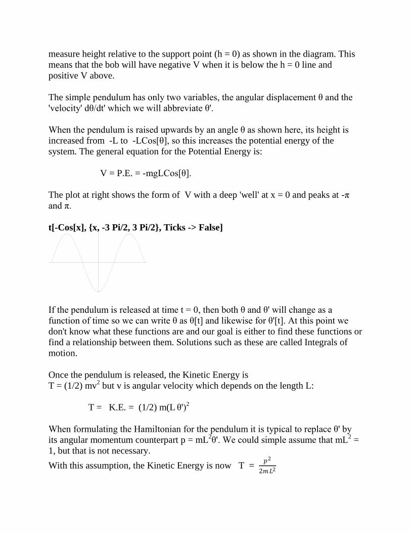
V = P.E. = -mgLCos[θ].
The plot at right shows the form of V with a deep 'well' at x = 0 and peaks at -π
and π.
t[-Cos[x], {x, -3 Pi/2, 3 Pi/2}, Ticks -> False]
If the pendulum is released at time t = 0, then both θ and θ' will change as a
function of time so we can write θ as θ[t] and likewise for θ'[t]. At this point we
don't know what these functions are and our goal is either to find these functions or
find a relationship between them. Solutions such as these are called Integrals of
motion.
Once the pendulum is released, the Kinetic Energy is
T = (1/2) mv2 but v is angular velocity which depends on the length L:
T = K.E. = (1/2) m(L θ')
2
When formulating the Hamiltonian for the pendulum it is typical to replace θ' by
its angular momentum counterpart p = mL2θ'. We could simple assume that mL
2 =
1, but that is not necessary.
With this assumption, the Kinetic Energy is now T = 𝑝2
2𝑚𝐿2

Hamiltonian = H[θ,p] = T + V = 𝑝2
2𝑚𝐿2 - mgLCos[θ]
The Hamiltonian equations of motion are
𝜕𝐻
𝜕𝜃 = -p' and
𝜕𝐻
𝜕𝑝 = θ'
These are partial derivatives which are necessary when dealing with more than one
variable. It means to regard all other variables as fixed when taking the derivative.
This works great for H because p only occurs in T and θ occurs in V. The second
equation above is really just the definition of p, but the first equation is valuable:
𝜕𝐻
𝜕𝜃 =
𝑑𝑉
𝑑𝜃 = mgLSin[θ] = -p' = -(mL
2θ')' = -mL
2θ''
So the 'Force' equation or the equation of motion is:
θ'' + 𝑔
𝐿 Sin[θ] = 0
We can see why this makes sense in the Force diagram at the right. The only force
acting on the pendulum is the force of gravity which acts straight down. But the
motion is constrained by the rod so the effective force is LmgSin[θ]. This force
acts over a distance L, so it is called a torque.
Newton's equations say that "Net force equals time rate of change of momentum"
which is usually written F = (mv)' but here the generalized momentum is p= mL2θ'
because the moment of inertia of the rod is mL2, so
Force = - LmgSin[θ]= ma = mL2θ''
(the negative sign is because the force is opposite that of θ)
As this example shows ,we could have derived the equation of motion without
explicitly using the Hamiltonian but it works wonders for multivariable problems.
The Hamiltonian formulation has many advantages over the direct use of Newton's
laws, because Hamilton's laws survive at almost all scales.
To see the connection between the Hamiltonian and twist maps or circle maps, we
will use Mathematica to solve this pendulum equation for a specific value of θ.
(The general solution involves elliptic integrals so to get a 'time series' θ[t] is a
little messy, Most college text books assume that θ is small and replace Sin[θ] with
θ. In that case it is easy to solve using integration.)
Poincare realized that it is possible to understand the behavior of a complex system
without an explicit time series solution. This seems alien to some engineers but for
those who want insight into complex systems it is often better to make a 'phase'
plot (also called a Poincare plot)
The first step in Poincare's program is to replace the second-order derivative with
two first order derivatives, using x= θ and y = θ'.
(Virtually all programs for numerical solutions of differential equations use this
process.) The equation of motion then splits into two equations:
(1) x' = y (just the definition of y)
(2) y' = - 𝑔
𝐿 Sin[x]
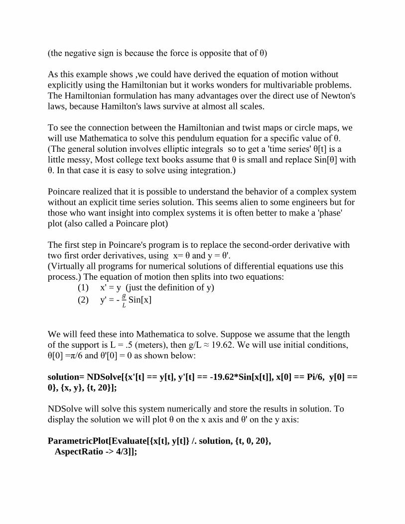
We will feed these into Mathematica to solve. Suppose we assume that the length
of the support is L = .5 (meters), then g/L ≈ 19.62. We will use initial conditions,
θ[0] =π/6 and θ'[0] = 0 as shown below:
solution= NDSolve[{x'[t] == y[t], y'[t] == -19.62*Sin[x[t]], x[0] == Pi/6, y[0] ==
0}, {x, y}, {t, 20}];
NDSolve will solve this system numerically and store the results in solution. To
display the solution we will plot θ on the x axis and θ' on the y axis:
ParametricPlot[Evaluate[{x[t], y[t]} /. solution, {t, 0, 20},
AspectRatio -> 4/3]];

Note that the point where this curve crosses the x axis has coordinates {Pi/6
≈.523,0}. These were our initial values for x and y and they determined the
solution curve. Points travel around this curve in a clockwise direction as the bob
starts out with negative velocity and then stops before returning with positive
velocity along the top half of the curve. The curve looks like an ellipse, but it is
not.
Different choices of initial conditions will yield a more complete 'phase plot' like
the one shown on the right. In this plot the inner curves are almost circular
because we chose g/L = 1. The wavy lines at top and bottom correspond to initial
conditions severe enough to make the bob complete a full rotation. The plots go on
forever left and right but they repeat every 2π because x is an angle.
Fixed Points
When studying the behavior of a dynamical system, the most important points are
the fixed points. If the system is defined using differential equations, these points
satisfy x'=0 and y' = 0, so once a system reaches a fixed point it stays there. The
Ideal Pendulum has two fixed points: x = 0,y = 0, and x = ± π, y = 0. That sounds
0.4 0.2 0.2 0.4
2
1
1
2

like 3 points but (+π,0) and (-π,0) are regarded as the same point, so take your pick,
it does not matter.
The origin {0,0}corresponds to the pendulum sitting straight down at rest. If the
pendulum is offset slightly,the phase plot will yield a circle or ellipse (nearly) so
this is called a 'center' or an elliptical fixed point. This is a stable fixed point
because nearby points do not diverge.
The point {π,0} and the matching point {-π,0} are very unstable because the
pendulum is sitting straight up. They are also called saddle points because points
converge in one direction and diverge in another. If you sit the pendulum straight
up and let it go, it would initially diverge, but in a 'perfect world' it would
eventually converge to that same point from the other direction.
We can see this on the phase plots. This 'perfect' orbit is called a 'separatrix'
because it separates the back-and-forth motion (librations) from the rotor motion
where the direction of motion never changes. This seperatrix is only an 'ideal' orbit.
The orbit could not be completed in any finite amount of time because the bob
would have to slow to zero velocity at exactly the right position. The seperatices
are very important from a theoretical point of view and for the pendulum, we can
use the Hamiltonian to find their equation, Points like {π,0} are also called
homoclinic points or 'snap-back' points because if you trace an 'ideal' orbit leaving
such a point, it will eventually return.
Finding Equations for the Energy curves
Every one of these curves corresponds a constant total energy H, so we can use the
Hamiltonian to find the curve.For example the seperatrix corresponds to x = π and
y = 0, so the total energy is H = mgL. This will allow us to find an exact equation
for the curves instead of an approximation. We can do this in the general case but
we will just do an example. The general case is shown in the right side-bar.
Example: Suppose m = 1, g = 9.81,L = .5, x[0] = π/6. Since y[0] = 0 the Kinetic
Energy component is 0:
H[π/6,0] = 0 - mgLCos[θ] = -(1)(9.81)(.5)Cos[π/6]= - 9.81
4√3

This is the energy level for the curve, so it yields a relationship between θ and θ':
𝑝2
2𝑚𝐿2 - mgLCos[θ] = H = -
9.81
4√3
Recall that p = mL2θ'. Substituting for m, g and L gives:
Cos[θ] = θ ′
2
4(9.81) +
√3
2
Take ArcCos (Cos-1
) of both sides and plot
ParametricPlot[{ArcCos[(y^2/39.24 ) + Sqrt[3]/2], y}, {y, -10, 10},
AspectRatio-> 3]
This curve is identical to the numerical estimate plotted earlier ArcCos has two
solutions and the Mathematica default is to plot the 'positive' one. The general
solution is shown in the right-hand side-bar as a contour plot.
ContourPlot[y^2/2 + 2*(1 - Cos[x]), {x, -Pi, Pi}, {y, -4, 4}]
ContourPlot[y^2/2 + 2*(1 - Cos[x]), {x, 0, 4 Pi}, {y, -4, 4}, AspectRatio ->
Automatic, ContourStyle -> Black, ContourShading -> None]
0.1 0.2 0.3 0.4 0.5
2
1
1
2
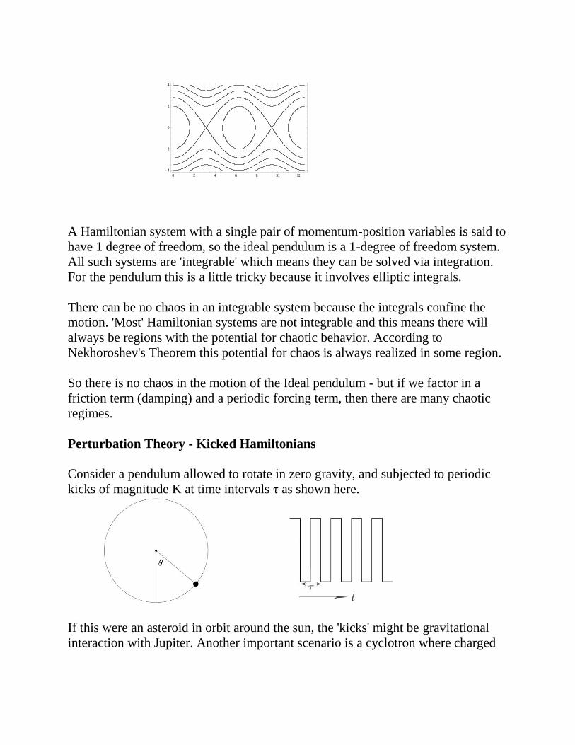
A Hamiltonian system with a single pair of momentum-position variables is said to
have 1 degree of freedom, so the ideal pendulum is a 1-degree of freedom system.
All such systems are 'integrable' which means they can be solved via integration.
For the pendulum this is a little tricky because it involves elliptic integrals.
There can be no chaos in an integrable system because the integrals confine the
motion. 'Most' Hamiltonian systems are not integrable and this means there will
always be regions with the potential for chaotic behavior. According to
Nekhoroshev's Theorem this potential for chaos is always realized in some region.
So there is no chaos in the motion of the Ideal pendulum - but if we factor in a
friction term (damping) and a periodic forcing term, then there are many chaotic
regimes.
Perturbation Theory - Kicked Hamiltonians
Consider a pendulum allowed to rotate in zero gravity, and subjected to periodic
kicks of magnitude K at time intervals τ as shown here.
If this were an asteroid in orbit around the sun, the 'kicks' might be gravitational
interaction with Jupiter. Another important scenario is a cyclotron where charged
0 2 4 6 8 10 12
4
2
0
2
4

particles are accelerated to high speed in a magnetic field created by an alternating
electric field.
The Hamiltonian is time dependent: 2
( , , ) cos ( )2 n
pH p t K n
I
t
where I is the moment of inertia of the pendulum, which we will scale to be 1, and
is the Dirac Delta function which yields pulses only when the input is 0 and this
occurs at time intervals τ , so ( ) ( )n
t K nt
is the periodic pulse stream shown
above.
From the Hamiltonian,we can see that the pulse stream alters the Potential Energy
at periodic intervals and this shows up in the system equations as a change in
Kinetic Energy:
The equations of motion are: sin ( )n
dpK n
dt
t
and
dp
dt
So the rotor receives a periodic torque of magnitude Ksinθ at time intervals ∆t = τ.
For the discrete equations, we can scale the intervals to get τ = 1. The effect of the
kth kick is to update p based on the current value of θ, so pk+1 = pk + Ksinθk.
Between kicks, the motion is force free so p is constant and the second equation
above says that θ is updated by p∆t = p , so θk+1= θk + pk+1.This gives the following
equations which describe the system just after the kth kick.
1 1
1
sin
sin sin
k k k k k k
k k k k k
p p K
p p K p K
These equations are called the Standard Map.
The Standard Map
1
1
sin
sin
k k k k
k k k
x x y K x
y y K x
When x plays the role of the angular variable θ and y plays the role of momentum
p. The determinant of the Jacobian is 1, so it is area preserving. Since the
perturbation is periodic modulo 2*Pi, it is common to scale x and K by 2*Pi and
plot x Mod1. Following normal convention we will plot both x and y Mod 1.
Std[{x_, y_}] := Mod[{y + (K/(2*Pi))*Sin[2*Pi*x] + x, y +
K/((2*Pi))*Sin[2*Pi*x]}, 1];

Example: K =0.971635406; gamma = (Sqrt[5]-1)/2;
Orbit1= NestList[Std, {0,gamma}, 1000]; Orbit2= NestList[Std, {0,1-gamma},
1000];
To get a range of initial conditions passing through the center of the plot:
VerticalScan = Flatten[Table[NestList[Std, {.5, y}, 1000], {y, 0, 1, .01}], 1];
Graphics[{AbsolutePointSize[1.0],Blue,Point[VerticalScan],Magenta,
Point[Orbit1], Point[Orbit2]},Axes->True]
This mapping is a paradigm for Hamiltonian chaos in the sense that it is an area
preserving map with divided phase space where 'integrable islands of stability are
surround by a chaotic component'. The two magenta orbits are remnants of the last
surviving invariant torus - with highly irrational winding number equal to the
Golden Mean. . As K increases past 0.971635406 and these curves break down,
there is no further impediment to large scale chaos in the central region.
The K = 0 case corresponds to an integrable Hamiltonian such as H(θ,p) = ωp2 so
the angular momentum p is constant and the Standard Map reduces to a circle map
(twist map) xk+1= xk + y with winding number y. The circles (tori) come in two
varieties depending on whether y/2π is rational or irrational. When K > 0, The
Standard Map simulates what happens to H when it is perturbed by periodic 'kicks'
of the form sinK x . So the Standard Map is a Poincare cross section of perturbed
twist map.

The fixed points are at {0,0} and {1/2,0}. The Jacobian is J =
𝜕𝑓₁
𝑑𝑥
𝜕𝑓₁
𝑑𝑦
𝜕𝑓₂
𝑑𝑥
𝜕𝑓₂
𝑑𝑦
= 1 1
cos 2 1 cos 2K x K x
At {0,0}, J =
1 1
1K K
so this is an unstable saddle
point as we can see above. At {1/2,0} J = 1 1
1K K
and this is a center for
(0,4)K
Therefore for K in this range, the motion in the vicinity of {1/2,0} is locally
conjugate to a rotation. These rotations are the cross sections of the 'tori' from the
Hamiltonian and we know that the curves with irrational winding numbers (like the
Golden Mean curve) are most likely to survive as the perturbations are increased.
At this resolution it is hard to tell which curves are rational and which are
irrational. Below is an enlargment of a central region showing the nesting of
rational and irrational curves
Moving outwards from the center means that the conjugacy may no longer be
valid. For small K, the set of surviving curves can be parametrized by a Cantor set,
so they form a continuium, but the regions between these irrational curves contains
rational rotations with periodic orbits such as the period 46 orbit above. Under
perturbations, the KAM Theorem says that tori which are 'sufficiently' irrational
will survive, while most 'rational' tori will break up into the resonant islands that
we see in the Standard map.
In 1969 Michael Henon at the Institute for Astrophysics in Paris devised a 'polar
form' of the Standard map. He notes that the map was "suggested by Siegel in
1956 in "Vorlesungen uber Himmelsmechanik, SpringerVerlag pg 203". This map
is very similar to the Moser Map discused earlier.
Example: The Henon Mapping - a discrete-time system
x[n+1] = x[n]*Cos[A] - (y[n]- x[n]2)*Sin[A]
x[n+1] = x[n]*Sin[A] + (y[n]+ x[n]2)*Cos[A]
In functional form it looks like:
H[{x_, y_}] = {x*Cos[A] - (y - x^2)*Sin[A], x*Sin[A] + (y - x^2)*Cos[A]}
To see whether it is area-preserving we need to take the Determinant of the
Jacobian J
J = D[H[{x,y}], {{x, y}}] =
{{Cos[A] + 2 x Sin[A], -Sin[A]}, {-2 x Cos[A] + Sin[A], Cos[A]}}
Det[J] ={Cos2[A] + Sin
2[A]} =1 (so the Henon mapping is area-preserving)
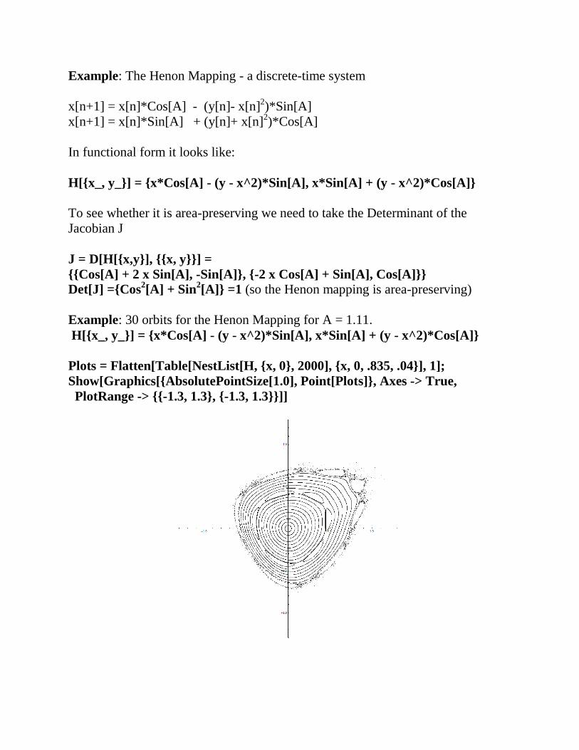
Example: 30 orbits for the Henon Mapping for A = 1.11.
H[{x_, y_}] = {x*Cos[A] - (y - x^2)*Sin[A], x*Sin[A] + (y - x^2)*Cos[A]}
Plots = Flatten[Table[NestList[H, {x, 0}, 2000], {x, 0, .835, .04}], 1];
Show[Graphics[{AbsolutePointSize[1.0], Point[Plots]}, Axes -> True,
PlotRange -> {{-1.3, 1.3}, {-1.3, 1.3}}]]

When this map starts to diverge, it does so exponentially, so we cannot go much
past {.835,0}. We will generate a more detailed plot below using the line of
symmetry. These plots mimic the phase plots for non-integrable Hamiltonian
systems It is a very complex interweaving of smooth invariant curves (the KAM
curves) and mode-locked islands which represent the breakdown of orbits with
winding numbers which are not 'sufficiently' irrational. In the example above there
is a prominent 6 to 1 resonance.
In the region between any two KAM curves there will be an infinite number of
resonant curves - because there are rational numbers between any pair of
irrationals and conversely. One way to get Mathematics to do exact arithmetic on
these orbits is to choose A of the form 2πx where x is rational.We will do this
below with A = Pi/3.
For small x values most initial points yield a smooth KAM curve but as x grows,
the system becomes unstable because of the nonlinear x2Sin[A] and x
2Cos[A]
terms.The center of the islands are stable periodic point just like the origin but the
these orbits decay like the origin and the region between the islands contain
unstable 'saddle point' like the {π,0} point for the pendulum. We can see 6 of these
homoclinic points below as they combine together to form a seperatrix.
The local neighborhood around a homoclinic fixed point can be expected to
contain chaotic orbits. For an area preserving map, these chaotic orbits show up as
a sea of dots - and this is what is called stochastic (random) behavior. The root of
this behavior is the sic condition which implies we cannot accurately track orbits
so they appear random.
Below is a plot with the same A value of 1.11. This plot chooses initial points on
the line of symmetry which has slope Tan[A/2]. The local homoclinic point is on
this line at about (.4383871, 271753}. We can see the outline of the 'seperatrix' but
the plot is only an approximation. The second plot zooms in on the homoclinic
point which is the red dot.
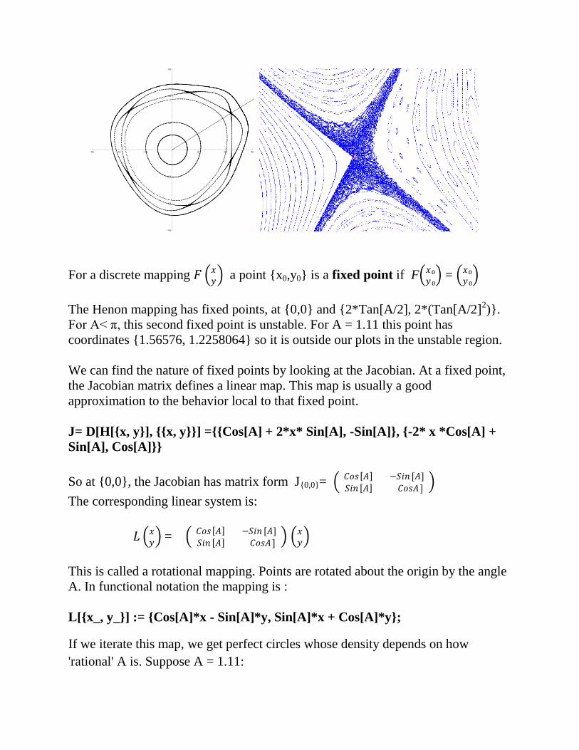
For a discrete mapping 𝐹 𝑥𝑦 a point {x0,y0} is a fixed point if F 𝑥₀
𝑦₀ = 𝑥₀
𝑦₀
The Henon mapping has fixed points, at {0,0} and {2*Tan[A/2], 2*(Tan[A/2]2)}.
For A< π, this second fixed point is unstable. For A = 1.11 this point has
coordinates {1.56576, 1.2258064} so it is outside our plots in the unstable region.
We can find the nature of fixed points by looking at the Jacobian. At a fixed point,
the Jacobian matrix defines a linear map. This map is usually a good
approximation to the behavior local to that fixed point.
J= D[H[{x, y}], {{x, y}}] ={{Cos[A] + 2*x* Sin[A], -Sin[A]}, {-2* x *Cos[A] +
Sin[A], Cos[A]}}
So at {0,0}, the Jacobian has matrix form J{0,0}= 𝐶𝑜𝑠 𝐴 −𝑆𝑖𝑛 [𝐴]
𝑆𝑖𝑛 𝐴 𝐶𝑜𝑠𝐴 ]
The corresponding linear system is:
𝐿 𝑥𝑦 = 𝐶𝑜𝑠 𝐴 −𝑆𝑖𝑛 [𝐴]
𝑆𝑖𝑛 𝐴 𝐶𝑜𝑠𝐴 ] 𝑥
𝑦
This is called a rotational mapping. Points are rotated about the origin by the angle
A. In functional notation the mapping is :
L[{x_, y_}] := {Cos[A]*x - Sin[A]*y, Sin[A]*x + Cos[A]*y};
If we iterate this map, we get perfect circles whose density depends on how
'rational' A is. Suppose A = 1.11:
0.6 0.4 0.2 0.2 0.4 0.6
0.6
0.4
0.2
0.2
0.4
0.6
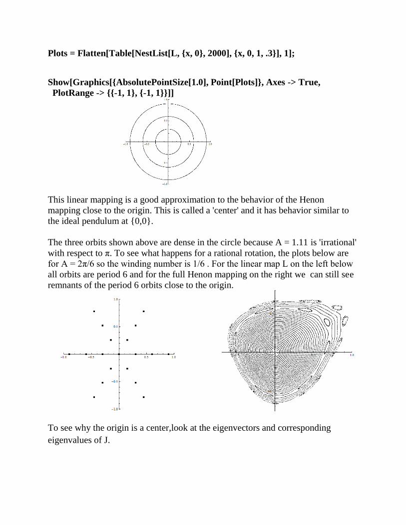
Plots = Flatten[Table[NestList[L, {x, 0}, 2000], {x, 0, 1, .3}], 1];
Show[Graphics[{AbsolutePointSize[1.0], Point[Plots]}, Axes -> True,
PlotRange -> {{-1, 1}, {-1, 1}}]]
This linear mapping is a good approximation to the behavior of the Henon
mapping close to the origin. This is called a 'center' and it has behavior similar to
the ideal pendulum at {0,0}.
The three orbits shown above are dense in the circle because A = 1.11 is 'irrational'
with respect to π. To see what happens for a rational rotation, the plots below are
for A = 2π/6 so the winding number is 1/6 . For the linear map L on the left below
all orbits are period 6 and for the full Henon mapping on the right we can still see
remnants of the period 6 orbits close to the origin.
To see why the origin is a center,look at the eigenvectors and corresponding
eigenvalues of J.
Definition:If A is a square matrix (with real coefficients), a nonzero vector v is an
eigenvector of A if for some scalar λ, the characteristic equation Av = λv has a
solution. The scalar λ is the corresponding eigenvalue.
Example: The Eigenvalues and Eigenvectors of the Henon Mapping at {0,0}
Eigenvalues[J{0,0}] = {Cos[A] - i Sin[A], Cos[A] + i Sin[A]}
Eigenvectors[J{0,0}] ={{-i, 1}, {i, 1}};
The eigenvalues are complex and conjugate to each other because they arise as
solutions to the same quadratic equation: Av = λv . The two eigenvalues are: λ1 =
Cos[A]-iSin[A] and λ1 = Cos[A] + iSin[A] . They have the same absolute value
|λ1| = |λ2| = 𝑆𝑖𝑛² 𝐴 + 𝐶𝑜𝑠² 𝐴 = 1
Since the eigenvalues at the origin are complex, the linearized mapping will
involve a rotation. With a 2 by 2 matrix A, there three types of rotations. If all
eigenvalues have absolute value < 1, points spiral inwards, If all eigenvalues have
absolute value >1, points spiral outwards, and if all eigenvalues have magnitude
equal to 1, points rotate about the fixed point as in our example above.
The Henon map is the composition of a rotation and non-linear 'shear' so H = L◦S
where L is the liearized mapping from earlier which we know is just a rotation by
A:
L[{x_, y_}] := {Cos[A]*x - Sin[A]*y, Sin[A]*x + Cos[A]*y};
And S is a 'shear' given by S[{x_, y_}] = {x, y - x2}. Shears are often introduced as
non-linear perturbations.

Do-It-Yourself Chaos
There are many common devices which are capable of exhibiting chaotic behavior.
Below is a list of devices and physical systems which have been known to exhibit
chaotic behavior.
•nonlinear stiffness in springs
•nonlinear friction or damping
•nonlinear boundary conditions, backlash
•fluid related forces, air convection
•nonlinear feedback in control systems
•diodes or transistors in electrical circuits
•nonlinear resistors, inductance, capacitance in electrical circuits
•magnetic forces
•systems with two well potentials
Swing Toys
These first two are 'toys' sold for a few dollars at specialty stores and airports. They
don't seem to have a common source or common names so we call them 'swing-
toys', They appear to come from Asia. In each case the design is the same. In the
hollow base there is an 8-volt battery which feeds an electromagnet. In the base of
the pendulum, there is a small magnet. When the pendulum swings past the base, a
sensor turns the electromagnet on briefly and the two magnets repel each other.
This small 'kick' keeps the pendulum going back and forth in a very periodic
fashion. The chaotic motion occurs with the secondary pendulum. They also have
small magnets to keep them from settling down into periodic motion.
It is amazing that this simple toy can run for many hours without ever repeating
itself. It is a little tricky to gather date from the secondary pendulum. Our best
success has been with motion sensors but it is necessary to filter out the motion of
the main bob. We discovered that for some designs there seem to be small non-
periodic variations in the electromagnetic current which might be an easier
parameter to measure. Since these variations are synchronized with the period of
the main bob they could allow construction of a Poincare section. A phase plot can
also be constructed from a time series x[t] using time delay techniques: plot x[t] vs
x[t + ∆t). A delay plot of a time series can generate a nice (pseudo) phase plot with
the right delay. Also a Fast Fourier Transform is easy to do and if the plot shows a
broad band of frequencies, it is most likely chaotic. This has been modeled with a
'kicked' Hamiltonian, which has also been used to model for the Tangent Map -
where the 'kick' is the movement of the point p to its image τ(p). Michael Berry at
the Willis Physics Laboratory in Bristol, U.K. published a study of this toy. He
called it the Bouncing Rotator.
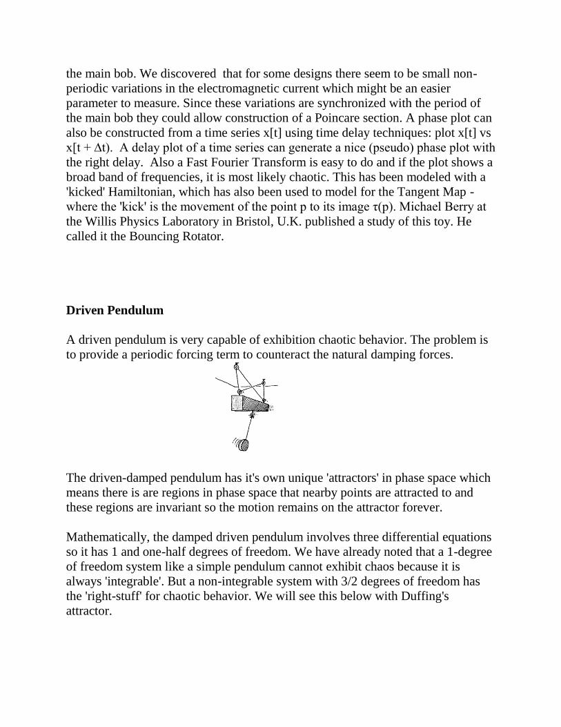
Driven Pendulum
A driven pendulum is very capable of exhibition chaotic behavior. The problem is
to provide a periodic forcing term to counteract the natural damping forces.
The driven-damped pendulum has it's own unique 'attractors' in phase space which
means there is are regions in phase space that nearby points are attracted to and
these regions are invariant so the motion remains on the attractor forever.
Mathematically, the damped driven pendulum involves three differential equations
so it has 1 and one-half degrees of freedom. We have already noted that a 1-degree
of freedom system like a simple pendulum cannot exhibit chaos because it is
always 'integrable'. But a non-integrable system with 3/2 degrees of freedom has
the 'right-stuff' for chaotic behavior. We will see this below with Duffing's
attractor.
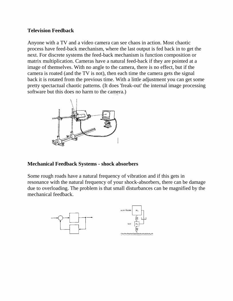
Television Feedback
Anyone with a TV and a video camera can see chaos in action. Most chaotic
process have feed-back mechanism, where the last output is fed back in to get the
next. For discrete systems the feed-back mechanism is function composition or
matrix multiplication. Cameras have a natural feed-back if they are pointed at a
image of themselves. With no angle to the camera, there is no effect, but if the
camera is roated (and the TV is not), then each time the camera gets the signal
back it is rotated from the previous time. With a little adjustment you can get some
pretty spectactual chaotic patterns. (It does 'freak-out' the internal image processing
software but this does no harm to the camera.)
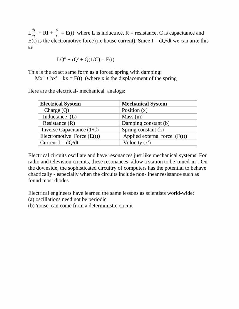
Mechanical Feedback Systems - shock absorbers
Some rough roads have a natural frequency of vibration and if this gets in
resonance with the natural frequency of your shock-absorbers, there can be damage
due to overloading. The problem is that small disturbances can be magnified by the
mechanical feedback.

Electrical Feedback Systems - the Space Shuttle
Today most feedback systems are electrical. Modern large planes use 'fly-by-wire'
which means that when the pilot makes an adjustment, electrical motors do the
actual work. This implies that there will be a delay from the moment a pilot turns
the plane and when the plane actually turns. If this delay is too long the pilot might
keep turning before he feels the effect of the previous motion, This can create a
run-away feedback. It plagued the early Space Shuttle designers because the pilots
felt that the system was hard to control until design engineers found the right level
of delay that pilots were comfortable with.
Electrical Circuits
There are many similarities between electrical circuits and mechanical systems. In
the days before powerful computers were available, people built electrical circuits
to simulate mechanical systems.
Example: Below is a simple RLC circuit (Resistance, Capacitance, Inductance)
When the switch is thrown a current will flow. Suppose Q is the charge on the
capacitor. By Kirchoff's law:
L𝑑𝐼
𝑑𝑡 + RI +
𝑄
𝐶 = E(t) where L is inductnce, R = resistance, C is capacitance and
E(t) is the electromotive force (i.e house current). Since I = dQ/dt we can arite this
as
LQ'' + rQ' + Q(1/C) = E(t)
This is the exact same form as a forced spring with damping:
Mx'' + bx' + kx = F(t) (where x is the displacement of the spring
Here are the electrical- mechanical analogs:
Electrical System Mechanical System
Charge (Q) Position (x)
Inductance (L) Mass (m)
Resistance (R) Damping constant (b)
Inverse Capacitance (1/C) Spring constant (k)
Electromotive Force (E(t)) Applied external force (F(t))
Current I = dQ/dt Velocity (x')
Electrical circuits oscillate and have resonances just like mechanical systems. For
radio and television circuits, these resonances allow a station to be 'tuned-in' . On
the downside, the sophisticated circuitry of computers has the potential to behave
chaotically - especially when the circuits include non-linear resistance such as
found most diodes.
Electrical engineers have learned the same lessons as scientists world-wide:
(a) oscillations need not be periodic
(b) 'noise' can come from a deterministic circuit

The Buckling Beam - Duffing's Two Well Oscillator
Jurgen Moser recommended a model for chaotic behavior called The Bucking
Beam. This is an easy model to construct at home.
Chaotic behavior often arises around unstable fixed points - like the homoclinic
points we saw with an inverted pendulum or Henon's mapping. Shown above are
three ways in which a thin beam can buckle. In each case the choice of direction
for the buckling is almost random. For example with the magnets, if we shake the
table or the support, the beam is just as likely to go one direction as the other. Now
suppose we have a periodic disturbance of this type - then the beam may never
settle down into a periodic pattern. At home you can model a periodic disturbance
by mounting a small motor on the top of the beam with a shaft that is slightly off
center. The speed of the motor can be controlled with a variable resistor.
On outer space the thin foils used as sun shields have been known to buckle in a
chaotic fashion due to the solar wind. Occasionally they will self-destruct. The
Buckling Beam is modeled by Duffing's equations
The two stable states of the beam are modeled by a potential function with two
'wells' as shown below. For the pendulum we had just one 'well' as shown on the
right.
If a ball is placed in such a well and subjected to periodic oscillations, the behavior
could become totally unpredictable depending on the frequency and amplitude of
the oscillations. The two-well oscillator can be modeled with a cubic potential
term:
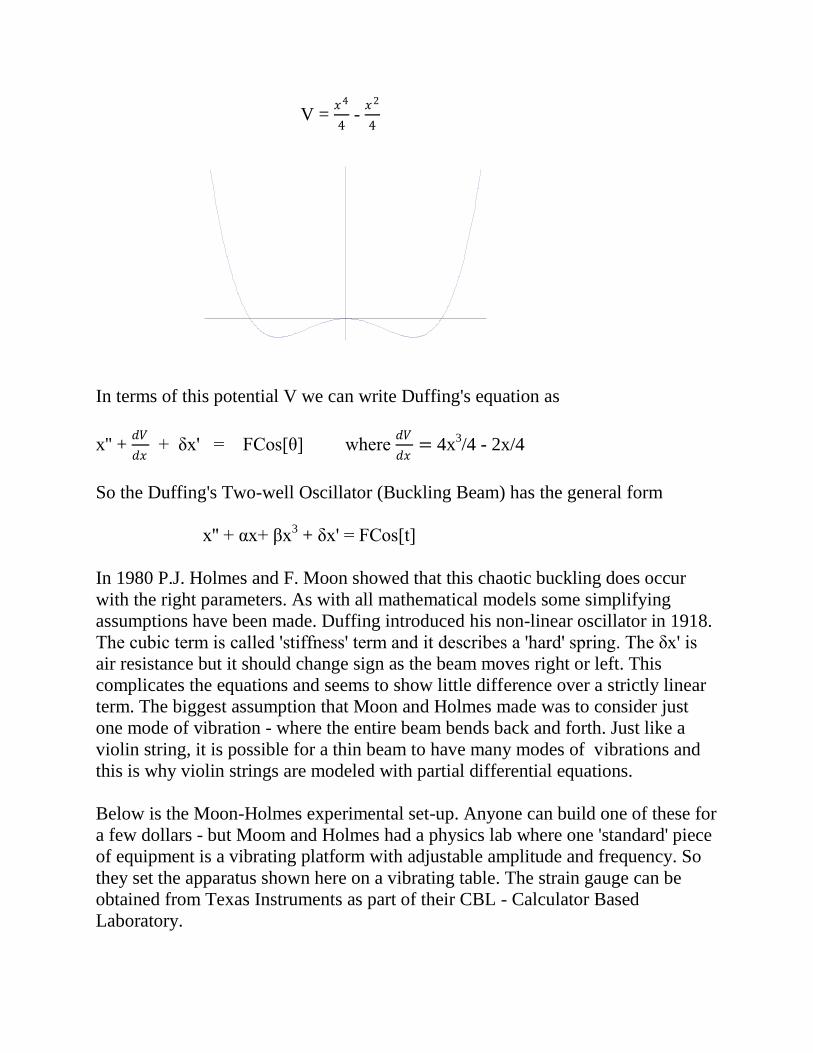
V = 𝑥4
4 - 𝑥2
4
In terms of this potential V we can write Duffing's equation as
x'' + 𝑑𝑉
𝑑𝑥 + δx' = FCos[θ] where
𝑑𝑉
𝑑𝑥= 4x
3/4 - 2x/4
So the Duffing's Two-well Oscillator (Buckling Beam) has the general form
x'' + αx+ βx3 + δx' = FCos[t]
In 1980 P.J. Holmes and F. Moon showed that this chaotic buckling does occur
with the right parameters. As with all mathematical models some simplifying
assumptions have been made. Duffing introduced his non-linear oscillator in 1918.
The cubic term is called 'stiffness' term and it describes a 'hard' spring. The δx' is
air resistance but it should change sign as the beam moves right or left. This
complicates the equations and seems to show little difference over a strictly linear
term. The biggest assumption that Moon and Holmes made was to consider just
one mode of vibration - where the entire beam bends back and forth. Just like a
violin string, it is possible for a thin beam to have many modes of vibrations and
this is why violin strings are modeled with partial differential equations.
Below is the Moon-Holmes experimental set-up. Anyone can build one of these for
a few dollars - but Moom and Holmes had a physics lab where one 'standard' piece
of equipment is a vibrating platform with adjustable amplitude and frequency. So
they set the apparatus shown here on a vibrating table. The strain gauge can be
obtained from Texas Instruments as part of their CBL - Calculator Based
Laboratory.
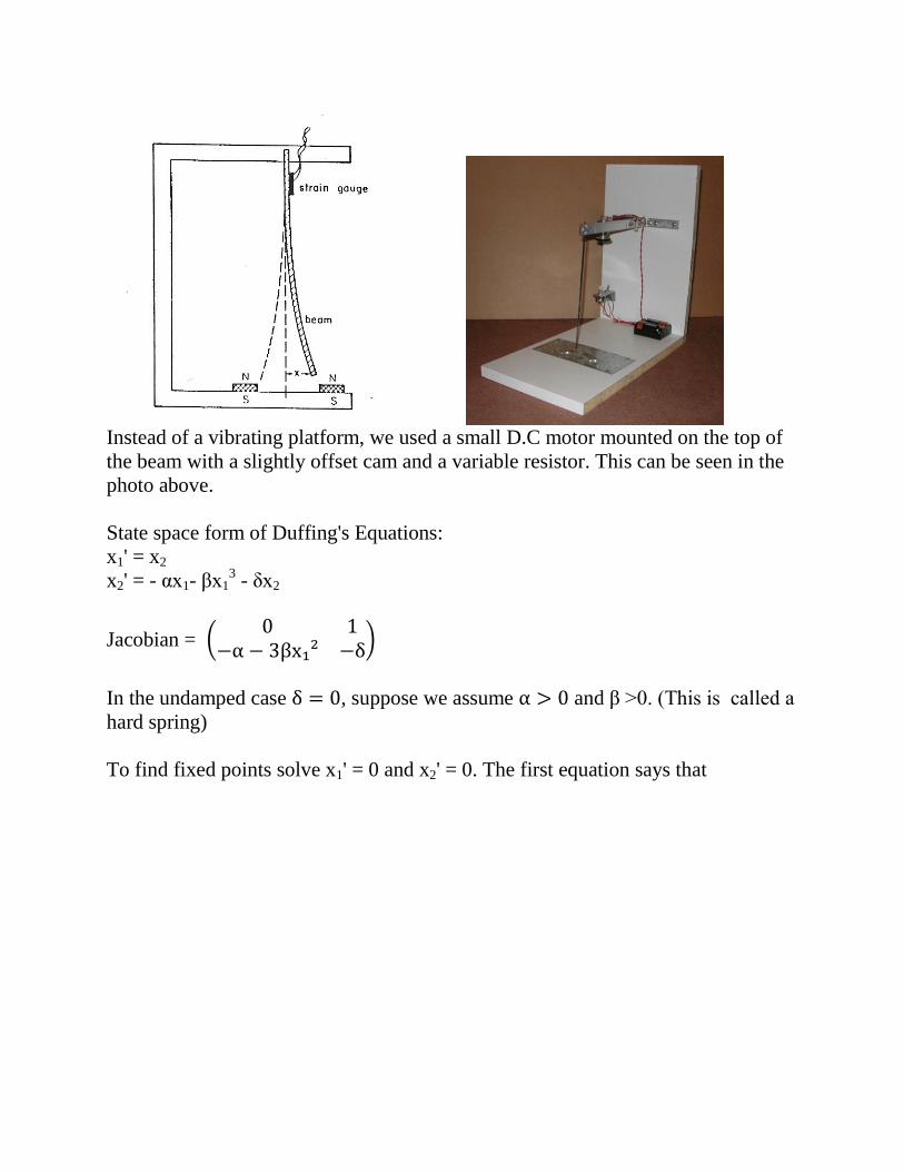
Instead of a vibrating platform, we used a small D.C motor mounted on the top of
the beam with a slightly offset cam and a variable resistor. This can be seen in the
photo above.
State space form of Duffing's Equations:
x1' = x2
x2' = - αx1- βx13 - δx2
Jacobian = 0 1
−α − 3βx₁² −δ
In the undamped case δ = 0, suppose we assume α > 0 and β >0. (This is called a
hard spring)
To find fixed points solve x1' = 0 and x2' = 0. The first equation says that

One way to model this at home is to use a short piece of track with a base for a
flexible ruler. The ruler can have adjustable weights, allowing it to flop over
equally in either direction. The challenging part is to provide an adjustable periodic
x2 = 0, and the second equation has just one real root which is x1 = 0. So we have
one fixed point at {0,0}with Jacobian 0 1−α 0
This is clearly a center. Below is a phase plot of x1 vs x2 at the origin
Now suppose we have a 'soft' spring with α > 0 and β < 0. We will assume α = 0
and β=-1.
The fixed point at the origin remains but now we have saddle points at {1,0} and {-
1,0}
J{0,0}= 0 1−1 0
J{1,0}= J{-1,0} = 0 12 0
Below is the new phase plot showing the two saddle points
Our real interest is in the Inverted Duffing Equation because it models an inverted
pendulum or beam. This is the case where α < 0 and β > 0. If we still assume that
damping is 0, the fixed points do not change but their eigenvalues get flipped
around with the origin being a saddle point and{1,0} and {-1,0} are now centers as
shown below
disturbance to the cart. Our solution was to use an old airplane motor and drive the
propeller with a D.C. motor.
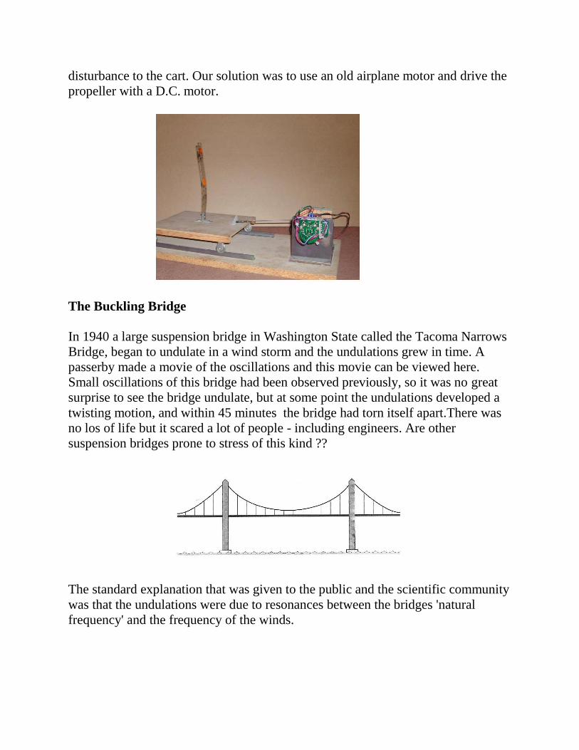
The Buckling Bridge
In 1940 a large suspension bridge in Washington State called the Tacoma Narrows
Bridge, began to undulate in a wind storm and the undulations grew in time. A
passerby made a movie of the oscillations and this movie can be viewed here.
Small oscillations of this bridge had been observed previously, so it was no great
surprise to see the bridge undulate, but at some point the undulations developed a
twisting motion, and within 45 minutes the bridge had torn itself apart.There was
no los of life but it scared a lot of people - including engineers. Are other
suspension bridges prone to stress of this kind ??
The standard explanation that was given to the public and the scientific community
was that the undulations were due to resonances between the bridges 'natural
frequency' and the frequency of the winds.

On closer examination, this explanation makes no sense. The main issue is that
winds do exhibit bouts of periodic behavior but there is no 'natural' frequency
which could nteract with the natural frequency of the bridge to make a resonance.
As pointed out in an extensive 1991 study by Engineers Robert Scanlon of Johns
Hopkins and Yusuf Billah of Princeton University, even if there was some wind-
induced resonance, it could not have caused the twisting oscillations observed in
winds of 42-miles-per-hour.
Scanlon and Billah believe the twisting oscillations which broke the bridge apart
came from the motion of the bridge itself. Even a slight initial slackening of the
cables at one location would induce an asymmetrical condition which could be
magnified through internal resonances. A computer simulation by Joseph
McKenna at the University of Connecticut and Alan Lazer of the University of
Miami seems to support this theory of non-linear shearing forces. (As mentioned
earlier the Henon mappings gets its non-linearity from a shear.)
In linear dynamics, the amplitude of oscillations of a system vary in proportion to
the magnitude of the input, but in non-linear systems there might be no correlation
between the two. This is an engineers nightmare. In the years since 1940 there
have been no recurrences of this disaster and this is due in part to the new Science
of Non-linearity.
A Dripping Faucet
The drippings of a faucet sometimes are periodic but then are often episodes of
non-periodic behavior. With the spigot adjusted properly this non-periodic can go
on for a long time and it is not difficult to find parameters where the dripping is
chaotic. The amazing thing is that the plots generated show 'bifurcations' which are
virtually identical to bifurcations found in simple 1-dimensional families of
mapings. This is 'universality' theme that appears throughout the study of non-
linear science. There are sometimes deep relationships here that we are only
begining to understand. One of the typical scenarios is this:
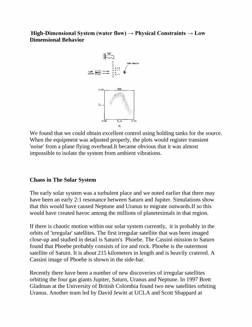
High-Dimensional System (water flow) → Physical Constraints → Low
Dimensional Behavior
We found that we could obtain excellent control using holding tanks for the source.
When the equipment was adjusted properly, the plots would register transient
'noise' from a plane flying overhead.It became obvious that it was almost
impossible to isolate the system from ambient vibrations.
Chaos in The Solar System
The early solar system was a turbulent place and we noted earlier that there may
have been an early 2:1 resonance between Saturn and Jupiter. Simulations show
that this would have caused Neptune and Uranus to migrate outwards.If so this
would have created havoc among the millions of planetesimals in that region.
If there is chaotic motion within our solar system currently, it is probably in the
orbits of 'irregular' satellites. The first irregular satellite that was been imaged
close-up and studied in detail is Saturn's Phoebe. The Cassini mission to Saturn
found that Phoebe probably consists of ice and rock. Phoebe is the outermost
satellite of Saturn. It is about 215 kilometers in length and is heavily cratered. A
Cassini image of Phoebe is shown in the side-bar.
Recently there have been a number of new discoveries of irregular satellites
orbiting the four gas giants Jupiter, Saturn, Uranus and Neptune. In 1997 Brett
Gladman at the University of British Colombia found two new satellites orbiting
Uranus. Another team led by David Jewitt at UCLA and Scott Shappard at

Carnegie Institute of Washington found new satellites orbiting Jupiter. These
discoveries were made possible by attaching new wide-field CCD cameras to large
telescopes.
The table below showing the current count is from the February, 2011 issue of
Astronomy
Planet Regular
Satellites
Irregular
Satellites
Total
Jupiter 8 55 63
Saturn 24 38 62
Uranus 18 9 27
Neptun
e
6 7 13
Some of these irregular satellites orbit far from the host planet but they are all
within the 'Hill sphere' of the host. The Hill sphere is the sphere surrounding the
planet with approximate radius
Where а is the semi-major axis of the smaller body and M is the mass of a
'competing' body (such as the sun). So the Hill sphere of the earth as about 1.5
million km compared to the moons orbit which is at .84 million km. In order for
the Earth to capture an asteroid, the asteroid would have to be within Earth's Hill
sphere -but this would not guarantee that the asteroid would have a stable orbit
around Earth. It seems that the stable part of the Hill sphere is somewhere inside
the inner half. The Hill sphere of Saturn is shown at left (from Astronomy,
February, 2011.)The space station or artificial satellites are much to small to have a
Hill sphere.
The Earth recently capture a small (15 meters wide) asteroid numbered 2006 RH120
but it only survived for about 4 orbits before returning to its orbit around the sun.
The dates were September 2006 to June 2007.
In 1982, the satellite Voyager 2 made a spectacular visit to Saturn. Its trajectory
brought it much closer to Saturn than it's predecessor, Voyager 1.

The only stable orientation of an ellipsoidal satellite would be a rotation about it's
longest axis like a football, and tidal friction would gradually force this spin axis to
be perpendicular to the plane of the orbit. The Voyager pictures show that the spin
axis is actually near the plane of the orbit rather than perpendicular to it. This is not
Before Voyager made contact with Saturn, it was believed that Saturn had 10
satellites. Voyager discovered that there were 15. And now the count has grown to
24 regular satellites and 38 irregular satellites. One of the more interesting of the
satellites observed by Voyager was Hyperion. Hyperion is irregular in shape and
roughly ellipsoidal with axes of approximately 190 km by 145km by 114km.
The image in the side-bar is was taken in 2005 by the Cassini mission. The orbit of
Hyperion lies outside the rings of Saturn and just beyond the orbit of the moon
Titan. The orbit is elliptical with a relatively high eccentricity ( = 0.1). This 10%
eccentricity, combined with it's irregular shape, causes tidal friction due to the
uneven forces of gravity over the surface of the satellite.. Over many eons, this
may have caused a chaotic tumbling of Hyperion as it rotates about Saturn. The
orbit itself appears to be quite regular with a period of 21.28 days but Voyager's
pictures seem to indicate an orientation period of about 13 days indicating that it
may have an erratic orientation as it orbits Saturn.
consistent with stable motion and it is believed that Hyperion is tumbling. There is
little doubt that at one time other satellites have behaved in a chaotic fashion but,
over the lifetime of the solar system, most satellites have been forced into
regularity by tidal forces of the parent body. Earth's moon is typical of many such
tamed satellites which now have orbits that match the rotation of the parent body.
Phobos and Deimos orbiting Mars probably once had chaotic orbits which may
have lasted on the order of 50 million years, but they now have regular periodic
orbits.
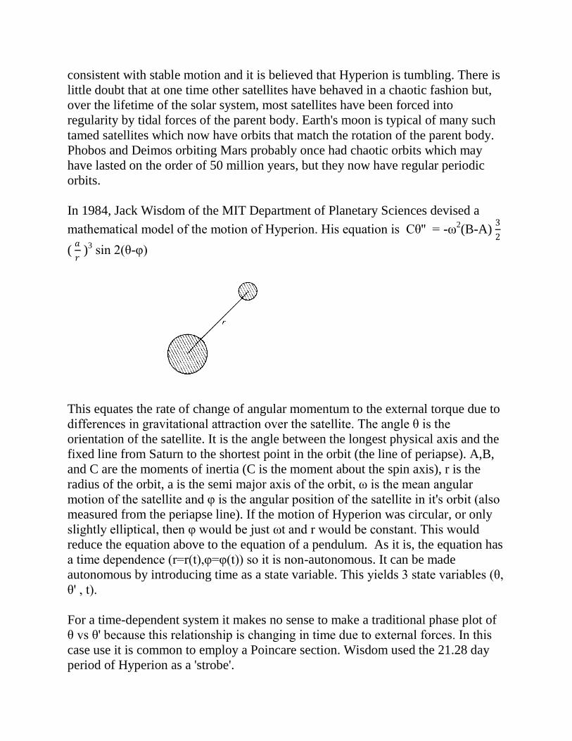
In 1984, Jack Wisdom of the MIT Department of Planetary Sciences devised a
mathematical model of the motion of Hyperion. His equation is Cθ'' = -ω2(B-A)
3
2
( 𝑎
𝑟 )3
sin 2(θ-φ)
This equates the rate of change of angular momentum to the external torque due to
differences in gravitational attraction over the satellite. The angle θ is the
orientation of the satellite. It is the angle between the longest physical axis and the
fixed line from Saturn to the shortest point in the orbit (the line of periapse). A,B,
and C are the moments of inertia (C is the moment about the spin axis), r is the
radius of the orbit, a is the semi major axis of the orbit, ω is the mean angular
motion of the satellite and φ is the angular position of the satellite in it's orbit (also
measured from the periapse line). If the motion of Hyperion was circular, or only
slightly elliptical, then φ would be just ωt and r would be constant. This would
reduce the equation above to the equation of a pendulum. As it is, the equation has
a time dependence (r=r(t),φ=φ(t)) so it is non-autonomous. It can be made
autonomous by introducing time as a state variable. This yields 3 state variables (θ,
θ' , t).
For a time-dependent system it makes no sense to make a traditional phase plot of
θ vs θ' because this relationship is changing in time due to external forces. In this
case use it is common to employ a Poincare section. Wisdom used the 21.28 day
period of Hyperion as a 'strobe'.

As illustrated below, he only plotted θ and θ' at time intervals of T = 21.28 days.
Note: In practice this meant that observers had to track Hyperion for extended
periods of time. Voyager was not designed to do this type of tracking. Three years
later an Earth-based study was conducted with a new generation of CCD camera.
This is reported below.
Poincare Section for the Motion of Hyperion - based on Mathematical Model
The plot below shows θ vs.θ' for a number of initial values,θ(0),θ'(0). Based on our
remarks above, θ has the form 2πT where T is the period of Hyperion. This is
typical for Poincare plots of nonlinear conservative systems in that some initial
conditions lead to regular motion while other initial conditions lead to chaotic
behavior. The central region is dominated by a single chaotic orbit while the
islands show orbits which where the rotation period is a multiple of the orbit
period. For example the large island would correspond to a synchronous orbit, like
that of our moon, where the rotation of the satellite just matched the orbital period.
The smaller island at the top would correspond to a rotational period where
Hyperion rotates exactly twice every orbit. The wavy lines are stable states where
the rotational period is not commensurable with the orbital period. These are called
quasi-periodic orbits.
Wisdom and his colleagues at MIT tried to find evidence of Hyperion's tumbling in
Voyages images, but the visual evidence was inconclusive. Based on their
simulations they estimated that the tumbling rate was rather slow, maybe on the
order of 10 days over two orbits of Saturn.
In 1987, to test the hypothesis of Hyperion's tumbling, the astronomer James
Klavetter spend three months at three different telescopes in Chile and the United
States. Even from the largest telescopes on earth, Hyperion cannot be observed
directly but telescopes can be fitted with sensitive light gathering equipment
(Charge Coupled Devices) which measure changes in the brightness of Hyperion
as a sign of tumbling. The problem is that the measurements have to be done on as
many consecutive nights as possible and they need to extend over at least 4.5 orbits
of Saturn which is about 13 weeks. Klavetter spent the first three weeks at Cerro
Tololo in Chili, then at week at Lowell Observatory in Flagstaff, Arizona and then
three months at the McGraw Hill Observatory in the Boston area.
The best data was obtained on the 2.4 meter McGraw Hill telescope but it took
months to interpret the data because the brightness of the night sky and Saturn and
nearby stars all had to be filtered out. This was done with a three dimensional
Fourier spectrum.
These same issues of stability arise in the analysis of satellites in orbit around the
earth. A cylindrical communications satellite may begin in orbit with rotation
about its short axis perpendicular to the plane of its orbit, but because of the
cylindrical shape, this rotation is not stable and tidal forces will work to align its
spin axis with the plane of the orbit itself so it will spin about it's longer axis in a
stable fashion. The problem is that in between the satellite may tumble erratically
like Hyperion.
There was indeed some evidence of brightness variation which would imply
tumbling. The hardest part was to find initial conditions for the model which would
yield the type of data observed. They were able to find a set of initial conditions
which yielded data similar to the observed. Of course if the motion is chaotic, the
simulation cannot predict with perfect accuracy any orbital characteristics, but it
can be used to obtain a qualitative match between actual and observed.
The best guess about how Hyperion got into this state is that it once had a stable
orbit with a much faster rotational period than it has now. At this point in time it
probably had its spin axis nearly perpendicular to the orbital plane like the moon
and the Earth but as tidal forces slowed the satellite, this orientation became
unstable because Hyperion was not spherical.

The Dynamics of The Human Electro-Encephalo-Gram
It is now widely known that the brain functions via neural connections which
transmit information with small electrical impulses. This means that sensitive leads
placed on the human skull can pick up electrical signals which may give some idea
of the inner workings of the brain. These tiny electrical signals were first
discovered by Canton in 1875 in small animals and by Berger in 1925 with
humans. These signals are now known as EEG signals which is an abbreviation for
electro-encephalo-gram.
Note:The early machines used to pick up the signals were called electro-encephalo-
graphs and so the output of these machines became known as electro-encephalo-
grams. The corresponding machine for measuring heart activity is called an
electro-cardio-gram and the signals are called electro-cardio-graphs or ECG (or
more commonly, EKG).
There are 4 standard regions for the EEG leads; two on each side of the brain. The
magnitude of the signals is small:on the order of microvolts. Since these signals are
generated on the brain's surface there is significant attenuation by the time they
reach the outer surface of the skull.The electrodes are pick up-devices which are
rubbed with conductive paste before being placed on the skull.
The EEG signals that are picked up by the electrodes are complex since they
represent large networks of neurons interacting with each other. But there are
underlying frequencies which can be detected by a frequency spectrum analysis.
On the left below are some time-series plots and next to them are 'delay plots'
where the time series data is plotted against itself with a specific time delay. In
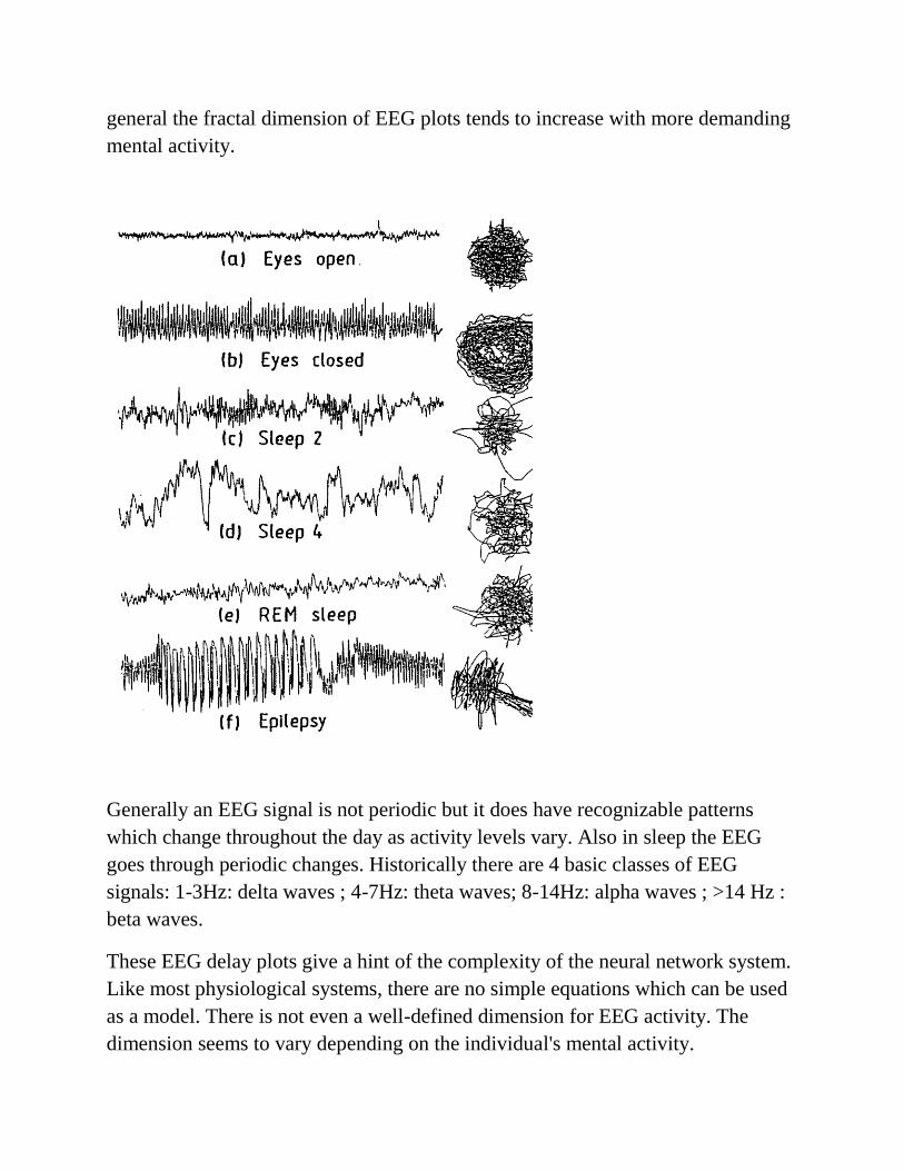
general the fractal dimension of EEG plots tends to increase with more demanding
mental activity.
Generally an EEG signal is not periodic but it does have recognizable patterns
which change throughout the day as activity levels vary. Also in sleep the EEG
goes through periodic changes. Historically there are 4 basic classes of EEG
signals: 1-3Hz: delta waves ; 4-7Hz: theta waves; 8-14Hz: alpha waves ; >14 Hz :
beta waves.
These EEG delay plots give a hint of the complexity of the neural network system.
Like most physiological systems, there are no simple equations which can be used
as a model. There is not even a well-defined dimension for EEG activity. The
dimension seems to vary depending on the individual's mental activity.


